Homogeneity assessment of Swiss snow depth series: comparison of break detection capabilities of (semi-)automatic homogenization methods

Knowledge concerning possible inhomogeneities in a data set is of key importance for any subsequent climatological analyses. Well-established relative homogenization methods developed for temperature and precipitation exist but have rarely been applied to snow-cover-related time series. We undertook a homogeneity assessment of Swiss monthly snow depth series by running and comparing the results from three well-established semi-automatic break point detection methods (ACMANT – Adapted Caussinus-Mestre Algorithm for Networks of Temperature series, Climatol – Climate Tools, and HOMER – HOMogenizaton softwarE in R). The multi-method approach allowed us to compare the different methods and to establish more robust results using a consensus of at least two change points in close proximity to each other. We investigated 184 series of various lengths between 1930 and 2021 and ranging from 200 to 2500 m a.s.l. and found 45 valid break points in 41 of the 184 series investigated, of which 71 % could be attributed to relocations or observer changes. Metadata are helpful but not sufficient for break point verification as more than 90 % of recorded events (relocation or observer change) did not lead to valid break points. Using a combined approach (two out of three methods) is highly beneficial as it increases the confidence in identified break points in contrast to any single method, with or without metadata.

1 Introduction

The quality of climate data time series analyses relies heavily on homogeneous input data, and such quality-controlled and homogenized climate data are needed to improve climate-related decision-making. Most decade- to century-scale meteorological time series are affected by inhomogeneities due to, for example, changes to instrumentation, changes to station location and observer practices, or changes in the local environment such as urbanization or plant growth (Tuomenvirta, 2001). Disentangling these break points from the underlying noise and variability in the data is challenging but crucial for improving confidence in any further analyses (e.g. Vertačnik et al., 2015). Accompanying metadata, if available, can be useful in helping to corroborate and verify breaks identified by statistical methods (Aguilar and Llanso, 2003). However, not every relocation or change in the station history necessarily leads to a break point in the data series in the first place.

There is no “one-method” solution when it comes to the detection of break points but rather a collection of statistical tools. Homogeneity tests can be broadly divided into “absolute” and “relative” methods. The former are applied directly to individual candidate stations to identify statistically significant shifts in the section means (referred to as breaks or change points), while relative methods entail comparison of correlated neighbouring stations with a candidate station to test for homogeneity. If reference series exist, a relative (rather than an absolute) approach where candidate series are compared to reference series is considered state of the art (Venema et al., 2012) in contemporary climate sciences as it allows the practitioner to eliminate any erroneous climatological shifts (Della-Marta and Wanner, 2006). Another advantage of some relative methods is that they do not require the reference series to be homogeneous themselves (Szentimrey, 1999; Caussinus and Mestre, 2004). Given the frequent occurrence of inhomogeneities in many climate time series, considerable efforts have been made to address the issue. These efforts by the community have produced a number of relative homogenization methods and toolboxes with varying degrees of user interaction and ease of application to choose from. PRODIGE (French for miracle) (Caussinus and Mestre, 2004) proved to be among the best-performing methods evaluated in the COST (European Cooperation in Science and Technology) Action HOME alongside ACMANT (Adapted Caussinus-Mestre Algorithm for Networks of Temperature series) (Domonkos, 2011), Climatol (Climate Tools) (Guijarro, 2018), USHCN (US Historical Climatology Network) (Menne and Williams, 2009), and MASH (Multiple Analysis of Series for Homogenization) (Szentimrey, 1999).

Efforts towards efficient break detection have been made for many meteorological variables such as temperature (e.g. Kuglitsch et al., 2012; Begert et al., 2008), precipitation (e.g. Begert et al., 2005; Coll et al., 2020), and phenological series (Brugnara et al., 2020) using various methods and tools. In the case of snow time series, however, only a few studies exist: Marcolini et al. (2017) investigated the use of the SNHT (standard normal homogeneity test; Alexandersson, 1986; Alexandersson and Moberg, 1997) for detecting breaks in mean annual snow depth. Marcolini et al. (2019) compared the use of the SNHT and PRODIGE for the break detection and subsequent homogenization of mean seasonal snow depth. Schöner et al. (2019) focused on trend analysis of seasonal mean snow depth in the Swiss–Austrian domain, using PRODIGE to identify inhomogeneous series in the records analysed. In our approach we choose to use multiple reference series processed using several modern relative methods, thereby increasing confidence in the results. As information concerning potential inhomogeneities is crucial in providing an accurate and reliable snow time series record, an in-depth homogeneity assessment of Swiss snow depth series is necessary.

For our study we used ACMANT (Domonkos, 2011, 2020), Climatol (Guijarro, 2018), and the semi-automatic tool HOMER (HOMogenizaton softwarE in R; Caussinus and Mestre, 2004; Domonkos, 2011; Guijarro, 2018; Picard et al., 2011) as they were all used for break detection purposes in recent studies: Kuya et al. (2021a) used Climatol for precipitation and HOMER for temperature (Kuya et al., 2021b); Noone et al. (2016) used HOMER for precipitation; and Coll et al. (2020) compared break detection performance of various methods including ACMANT, Climatol, and HOMER. Climatol is based on the SNHT (Alexandersson and Moberg, 1997) and recommended by Coll et al. (2020) for detecting breaks in precipitation series. HOMER is the extension development of and direct successor to PRODIGE and therefore is one of the most used homogenization methods in climate sciences. In addition it provides the homogenization practitioner with more operational freedom (in terms of configuration possibilities) than Climatol or ACMANT. Applying the different methods to Swiss snow depth time series and experimenting with various configurations allow us to investigate the suitability of the different set-ups and to provide a homogeneity assessment of the manual Swiss snow observation network.

Benchmark analyses of various methods exist for temperature and precipitation at both monthly and daily resolutions (e.g. Venema et al., 2012; Killick et al., 2021); however, no clear favourite has emerged. In addition, the use of Climatol (based on the SNHT) and HOMER (based on PRODIGE) allows for a more direct comparison with work already undertaken to assess homogeneity and break detection for snow time series in the Alps (Marcolini et al., 2017, 2019; Schöner et al., 2019). Furthermore, this in-depth analysis of Swiss snow series allows for the identification of suspicious or erroneous data in the series analysed which would otherwise have escaped detection. The process of homogenization can be described in three steps: break detection, attribution (verification of break points), and correction. In this study, we focus on the first step and touch upon the second. To focus our study, our research questions are as follows:

1. Which method or set-up works for break point detection in (Swiss) snow depth time series?

2. Is there any elevation dependence affecting the capability of the methods for break point detection?

3. Are the detected break points consistent with changes inferred from available metadata?

4. How homogeneous (in terms of detected break points) are the Swiss snow depth series investigated in our approach?

5. Are break point results similar for different snow cover variables (average snow depth and days with snow cover)?

The paper is organized as follows: Sect. 2 introduces the data set, and Sect. 3 details the methods used for the analyses. Results are presented in Sect. 4 and discussed in Sect. 5, and conclusions are drawn in Sect. 6.

2 Data

Our data consist of a newly compiled set of manually measured Swiss snow depth (HS) series obtained by the Federal Office of Meteorology and Climatology (MeteoSwiss) and the WSL Institute for Snow and Avalanche Research SLF. Manual snow measurements are conducted every morning between November and April at designated measurement fields with an observer reading off the snow depth from a graduated fixed stake; see Buchmann et al. (2021b) for more information. A favourable unique feature of using these manual snow depth measurements in Switzerland is that the instrument (graduated snow stake) and the general measurement procedure have not changed (Haberkorn, 2019), thereby eliminating one potential source of inhomogeneity in the records. We evaluated all the available series in the archives with data recorded between 1931 and 2021. Selection criteria were that time series have to be longer than 30 years and have at least 80 % complete data between November and April, and entirely missing single years were also allowed. Applying these criteria resulted in a data set of 184 station time series, distributed widely over Switzerland, from 200 to 2500 m a.s.l. Figure 1 shows the location and distribution of the stations used in this study (a list of all stations can be found in Table S1 in the Supplement). We use monthly (November–April) mean snow depth and monthly sums of days with snow on the ground for every hydrological year (November of the last year to April of the current year) as input data for the application of the break detection methods and set the remaining 6 months to zero. Days with snow on the ground are defined as days with snow depth equal to or greater than 1 cm. The final outputs used in the break point analysis were annual time series of winter mean snow depth (HSavg) and snow cover duration (dHS1).

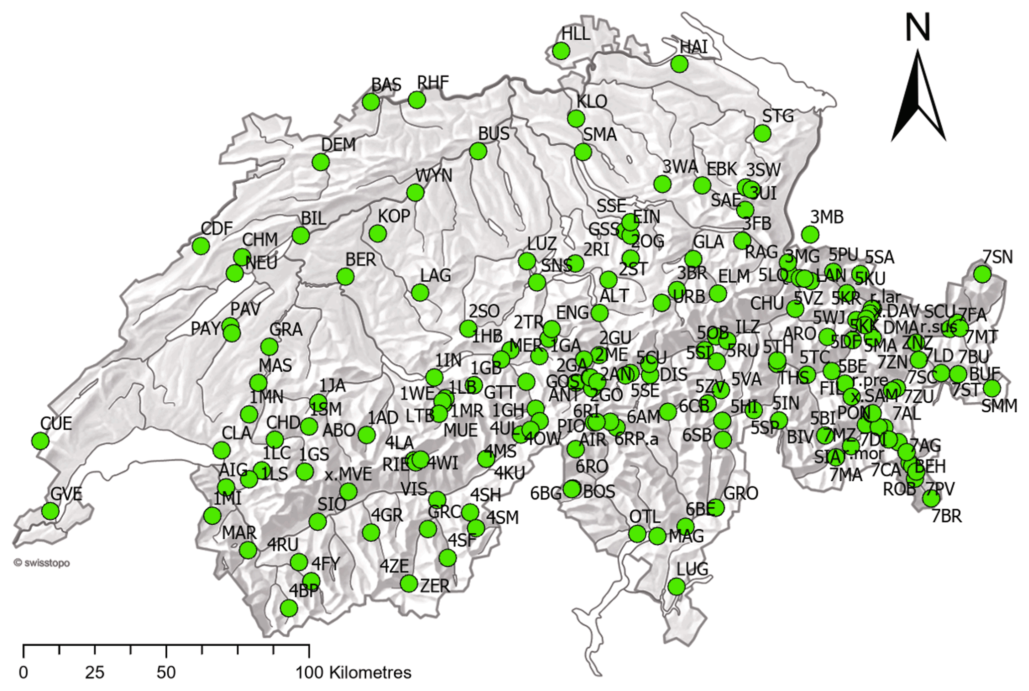
Figure 1 Map of Switzerland showing the distribution of the 184 stations used in this study.

Metadata

Since the instruments for manually measuring snow depth have not changed over our period of analysis, this allowed a clearer focus on other metadata components, such as coordinate changes as a proxy for station relocation and observer changes. Such information is generally available and was compiled from various sources (station records, archives, and operational databases). Unfortunately, for the MeteoSwiss network the exact locations of the snow measurements can differ from the coordinates of the associated meteorological station, and especially in the early days, MeteoSwiss did not record snow-specific coordinates. Moreover, the quality differs from station to station and is generally more vague for older periods (greater than 30 years) in the station records (Aschauer and Marty, 2020). Our metadata are not perfect (i.e. there is missing or incomplete information for some records); however, they are unlikely to be completely wrong and may offer some corroborative information for any breaks detected. Metadata are therefore used as additional verification for the identified break points where applicable/available with a tolerance of ±2 years.

3 Methods

3.1 Break detection algorithms

3.1.1 HOMER

HOMER is a collection of functions for break point detection and homogenization. The pairwise comparison (PRODIGE) is based on a penalized likelihood criterion (Caussinus and Lyazrhi, 1997) and is composed of optimal segmentation in conjunction with dynamic programming (Hawkins, 2001). Further methods are joint segmentation based on Picard et al. (2011) and ACMANT detection (Domonkos, 2011). We used pairwise comparison for our analyses because ACMANT detection depends on a seasonal cycle and Gubler et al. (2017) reported issues with HOMER's joint segmentation module. Coll et al. (2020) highlight that HOMER has its disadvantages when dealing with incomplete data, particularly when the missing data comprise contiguous blocks earlier or later in a series. For this reason the WMO Task Team on Homogenization recommends a missing data tolerance of 15 years for HOMER (WMO, 2017). However, as we are using mainly complete series and solely focus on pairwise detection, our analyses should not be affected. Network neighbourhoods in HOMER are constructed using station selection criteria, based on either distance or first-difference correlations. Here we used a minimum correlation threshold of 0.8 (empirical values) and a minimum number of five reference series (similarly to PRODIGE). In practice this means that if no reference series with correlations ≥ 0.8 are found for a particular candidate series, the five next best correlated stations are returned instead and, if more than five series exist with correlations ≥ 0.8, all are displayed.

Table 1 Settings for HOMER, ACMANT, and Climatol.

HOMER is semi-automatic insofar as it provides the user with a set of graphical difference series whereby the candidate series are compared to the reference series in each of the sub-networks based on the selection criteria applied. For each candidate and reference series in the derived sub-networks, any breaks detected are displayed to help inform subsequent adjustment decisions by the user. Difference series in HOMER can be defined in two ways: either the candidate minus reference (Diff-mode) or the candidate divided by reference (Ratio-mode). As our data are skewed due to the seasonal nature of snow cover data and limited at zero (no negative snow depth), we used Ratio-mode instead of differences (details in Table 1). Break points are interpreted as valid if they occur in more than half of the first five valid (with standard deviation of the noise (sigma) smaller than 0.3 and similar length and geographical origin to candidate series) reference series (i.e. three out of five), within an uncertainty of ±2 years, meaning that breaks are accepted as valid if they occur within ±2 years of each other in at least three reference series. The ±2 years is adopted from Kuglitsch et al. (2012). Venema et al. (2020) pointed out that parallel analyses of statistically or geographically relevant station data are the best solution for identifying breaks in time series. Some of the investigated snow time series are parallel series (Buchmann et al., 2021b), and if a break point is suggested in such a parallel candidate–reference series, it is double counted. In cases where some of the first 5 reference series selected do not cover the whole time period of the candidate series, the next longest series with sigma smaller than 0.3 might be included in the analysis. Furthermore, break detection was set to “annual”. Once the potential break points are adjusted based on operator interpretation and re-entered, HOMER is run again to calculate the break magnitude correction factors for each station.

3.1.2 ACMANT

ACMANT (Domonkos, 2011; Domonkos and Coll, 2017) is the most automatic of the homogenization methods used in this study, which means hardly any parameters can be changed by the user. Reference series are constructed via correlations between candidate and reference series with a fixed minimal correlation of 0.4. For this study we used ACMANTv4.3 (Domonkos, 2020) run in standard precipitation mode (see Table 1). Break points and the associated break magnitude corrections applied by ACMANT are retrieved from an automatically produced file. Automatic networking (AN) has been developed (Domonkos and Coll, 2019) as a preparatory operation for homogenizing data sets of more than 40 series (as is the case with the network here) with the ACMANT method. In AN, a specific network is constructed for each candidate series which provides optimal spatial comparison with the candidate series always in the centre of the network (Domonkos and Coll, 2017).

3.1.3 Climatol

In contrast to HOMER and ACMANT, Climatol uses composite reference series and detects breaks one by one with the standard normal homogenization test (SNHT; Alexandersson and Moberg, 1997) applied to anomaly series between candidate and reference series to detect break points. Anomalies are normalized through either the subtraction of or division by series averages, with the latter approach being recommended for skewed data series such as precipitation. Missing values are automatically infilled using values from neighbouring stations, thus allowing the method to compare series that do not share an intact data period prior to this adjustment. There are no pre-defined neighbourhoods as in HOMER, but a distance criterion is available to geographically confine the potential reference series (see Guijarro, 2018, and Coll et al., 2020, for more detail). Reference series are defined based on geographical proximity (Luna et al., 2012) using Euclidean distances. By default, the vertical coordinates in metres carry the same weight as the horizontal coordinates in kilometres. To account for the influence of elevation as a key control on snow, the scale parameter (wz) was adjusted so that elevation counts 100 times more, in practice meaning an elevation difference of 500 m is equivalent to a horizontal distance of 50 km in the approach used here. Climatol also provides an exploratory analysis of the data, which is necessary to properly set the parameters listed in Table 1. Once the parameters are set, Climatol can be run to produce an output file with suggested break points for each station. Break magnitude corrections are calculated as the change in mean before and after homogenization as Climatol does not automatically provide these values.

3.2 Evaluation of break detection algorithms

We define valid break points as break points detected at concordant times for any given series by at least two out of three independent methods within a tolerance of ±2 years regardless of metadata. As an additional measure, we only accepted as valid those break points identified within 5 years of either the beginning or the end of a series to agree with procedures used in Kuya et al. (2021a). The break points detected were then compared to available metadata where applicable; this metadata information was the decisive factor used to attribute the exact year of break points. In the case of those series where no metadata information was available, either the common year detected by a majority of the methods or the first occurrence of a concordant break point within the defined tolerance threshold was used.

To evaluate the performance and set-up of each method, their suggested break magnitude corrections and their contributions to concordant break points (number of valid break points compared to total number of detected break points) were measured and compared. To test whether break point detection depends on elevation or the “amount of snow”, detected breaks are compared to both station elevation and climatological (calculated for the entire period) snow values (i.e. mean HSavg). To assess how many valid break points can be explained by metadata and to see whether either station relocations or observer changes are more prone to cause detectable breaks, we compared the concordant break points to records in the station history.

Using this combined approach of integrating the break point information from the various methods alongside the information from metadata allows us to more confidently estimate the homogeneity of the Swiss snow network. The main focus is on breaks in HSavg; however, the opportunity to use dHS1 alongside HSavg as a complementary break point detection approach is discussed in Sect. 4.3. Series without any detected break points or break points detected by only one method are considered homogeneous; series with break points detected by at least two out of three methods (with or without metadata support based on our criteria) are considered inhomogeneous.

We are using HOMER 2.6, ACMANTv4.3, and Climatol 3.1.1; all analyses were run on a Windows system with R 4.1.1 (R Core Team, 2021).

4 Results

4.1 Comparison of method performances

4.1.1 Number of detected break points

To assess and be able to compare the three methods, we added up all the detected break points separately for each method and grouped them into time periods to investigate the temporal distribution of the break occurrences between the methods. Here we found ACMANT returning the largest number of detected break points with 170 breaks in 98 of the 184 series. The total numbers of break detections for Climatol (61 in 54) and HOMER (32 in 30) are significantly smaller than the ACMANT break detections. Table 2 and Fig. 2a summarize the overall break detection frequencies between the three methods. Figure 2b shows the temporal distribution of the detected break points between the methods. Based on this summary ACMANT detects the maximum number of break points between 1970 and 1980, whereas for Climatol and HOMER the 1980s is the decade associated with most detections. This suggests that ACMANT seems to be more sensitive in detecting changes than Climatol and HOMER, and the time period associated with the maximum number of break detections is coincident with the period where the maximum number of station records is available.

Table 2 Comparison of detected break points for each individual method. A valid break point means it was detected by at least two out of three methods. The complementary category uses break points from both dHS1 and HSavg (six break points are identical).

Figure 2 (a) Number of break points identified with ACMANT, Climatol, and HOMER for a total of 184 stations. (b) Number of break points and year of detection retrieved from ACMANT, Climatol, and HOMER for a total of 184 stations. The number of available series per decade is indicated with black dots and a corresponding right y axis. All results are for HSavg.

4.1.2 Break magnitudes and detection capabilities

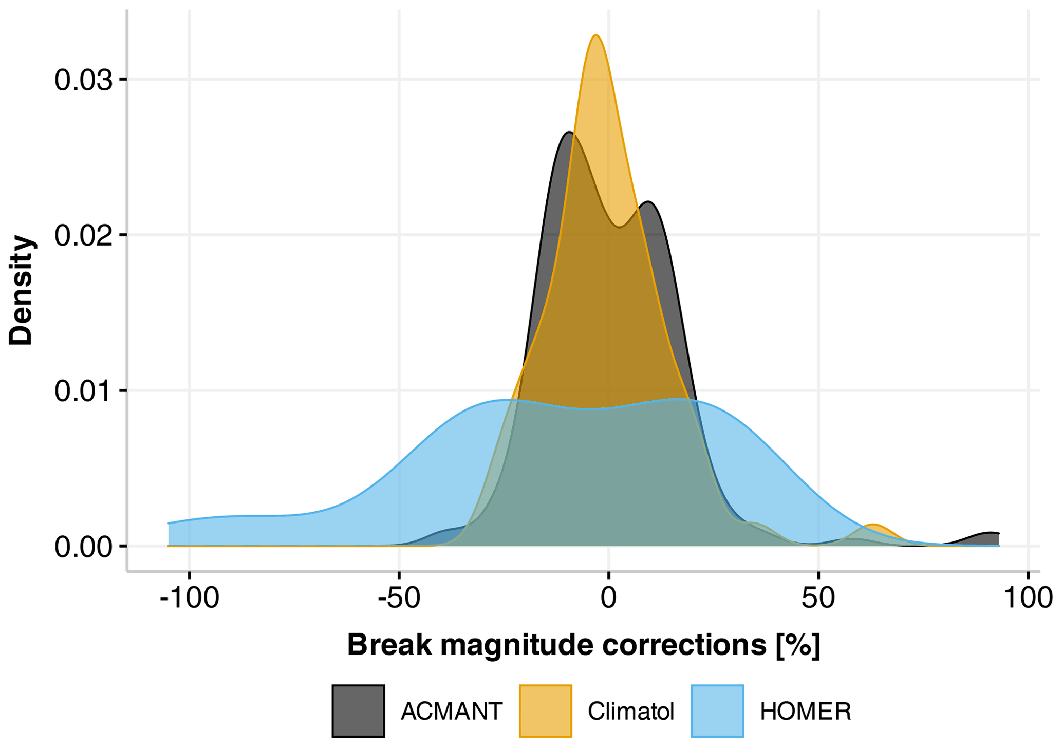
To investigate the sensitivity of the break detection capacity, the break magnitude corrections for all identified breaks are analysed across the methods. Figure 3a shows the number of detected breaks and their corresponding break magnitude correction categories. The majority of break magnitude corrections are distributed between 10 %–19 % (ACMANT and Climatol) and 20 %–29 % (HOMER). In contrast to ACMANT and Climatol, HOMER detects very few breaks with magnitude corrections below 10 %. This again indicates that ACMANT detects the most break points, including those of lower magnitude, whereas HOMER identifies fewer but higher-magnitude breaks. Climatol tends to mirror the pattern of ACMANT break point detection but with fewer detections overall. Figure 4 provides density distribution plots of the break magnitude corrections for the three methods separately. Here we found almost normal distributions for the Climatol and ACMANT break magnitude density distributions with a peak around 0 (suggesting no or very small corrections). The break magnitude distribution for ACMANT is bimodal with a local minimum at 0, reflecting more low-magnitude negative corrections than positive ones. The distribution of the break magnitude corrections for HOMER on the other hand is more uniform with no obvious peak. This reinforces that HOMER not only detects fewer break points than Climatol or ACMANT overall but also generally detects larger-magnitude breaks, a situation reflected in the broader distribution of break magnitude corrections.

Figure 3 (a) Absolute break magnitude corrections and their distribution for ACMANT, HOMER, and Climatol. (b) Break magnitude corrections versus station altitude. (c) Break magnitude corrections against mean HSavg. Valid break points are bold.

Figure 4 Density plots for break magnitude corrections for ACMANT, Climatol, and HOMER.

4.1.3 Elevation and amount-of-snow dependencies

The availability (as well as quality) of suitable reference series for each candidate station is key for a proper break point detection. Snow distribution in Switzerland is highly elevation-dependent, and our stations range from 200 to 2500 m a.s.l. To test the hypothesis that lower stations might not have enough suitable reference series for proper break point detections, a possible elevation dependence is investigated. To explore a possible altitudinal or amount-of-snow influence on the break detection capability of the methods, the break magnitude corrections of the identified break points were compared to station elevation and climatological HSavg (mean over the entire period of the available records). This comparison of break detections with elevation found fewer break points below 500 and above 1800 m a.s.l. than between 1300 and 1700 m a.s.l., whereas in comparison to the climatological HSavg, no clear pattern is visible. For these comparisons all three methods exhibited similar break detection patterns. Figure 3b and c plot these relationships separately, while Fig. 5 summarizes the relationship between station elevation and climatological HSavg for every station where break points were detected.

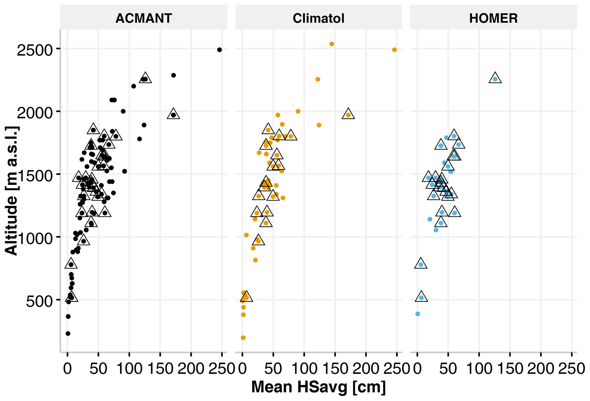
Figure 5 Break points in relation to station altitude and mean HSavg. Valid break points, identified by at least two methods, are marked with black triangles.

4.2 Concordant break points in HSavg

As the location and magnitude of break points obtained from the individual methods differed, for the remainder of the analysis only concordant break points (identified across all three methods) are considered. In this approach only breaks identified by at least two of the methods and obtained within ±2 years are considered to be valid. The set of valid break points based on these criteria are shown in Table 3. This approach identified 31 break points in 30 series for HSavg, with only one series showing multiple break points detected across all three methods. The majority of valid break points were found with a combination of ACMANT and HOMER, whereas no break points in HSavg were found with only Climatol and HOMER. Figure 6 summarizes the method combinations which led to break points being assessed as valid based on the criteria, while Fig. 7 summarizes the stations with identified inhomogeneities based on these same criteria. Multiple detections for series based on these criteria being applied across all three methods indicate that 83 % of the 184 Swiss snow series analysed can be considered homogeneous. However, the individual contributions to valid break points based on these selection criteria is different for each method, and these are summarized in Table 2. ACMANT and Climatol contribute to the detection of 18 % and 28 % respectively of valid break points based on our selection criteria, whereas HOMER accounts for 72 % of the detections. To further support the break points with reference to the available metadata (either station relocation or observer changes), the break points obtained across the methods were compared to any recorded changes in the station history. This comparison with the available metadata found that 22 of the 31 detected break points were supported by metadata and that of these 19 were due to station relocation while 3 could be attributed to a change of observer. The remaining 11 break points had no metadata support in the station histories. Figure 7 (as well as Fig. S1 in the Supplement) summarizes the metadata information supporting the valid break points. This strongly suggests that station relocation is a likely explanation for the majority of the supported inhomogeneities detected in the snow series records analysed here.

Table 3 List of valid break points concordantly identified in 184 investigated Swiss snow time series. Stations are ordered according to break year, and series with break points identified in both HSavg and dHS1 are marked bold. Combination code refers to ACMANT (A), Climatol (C), and HOMER (H).

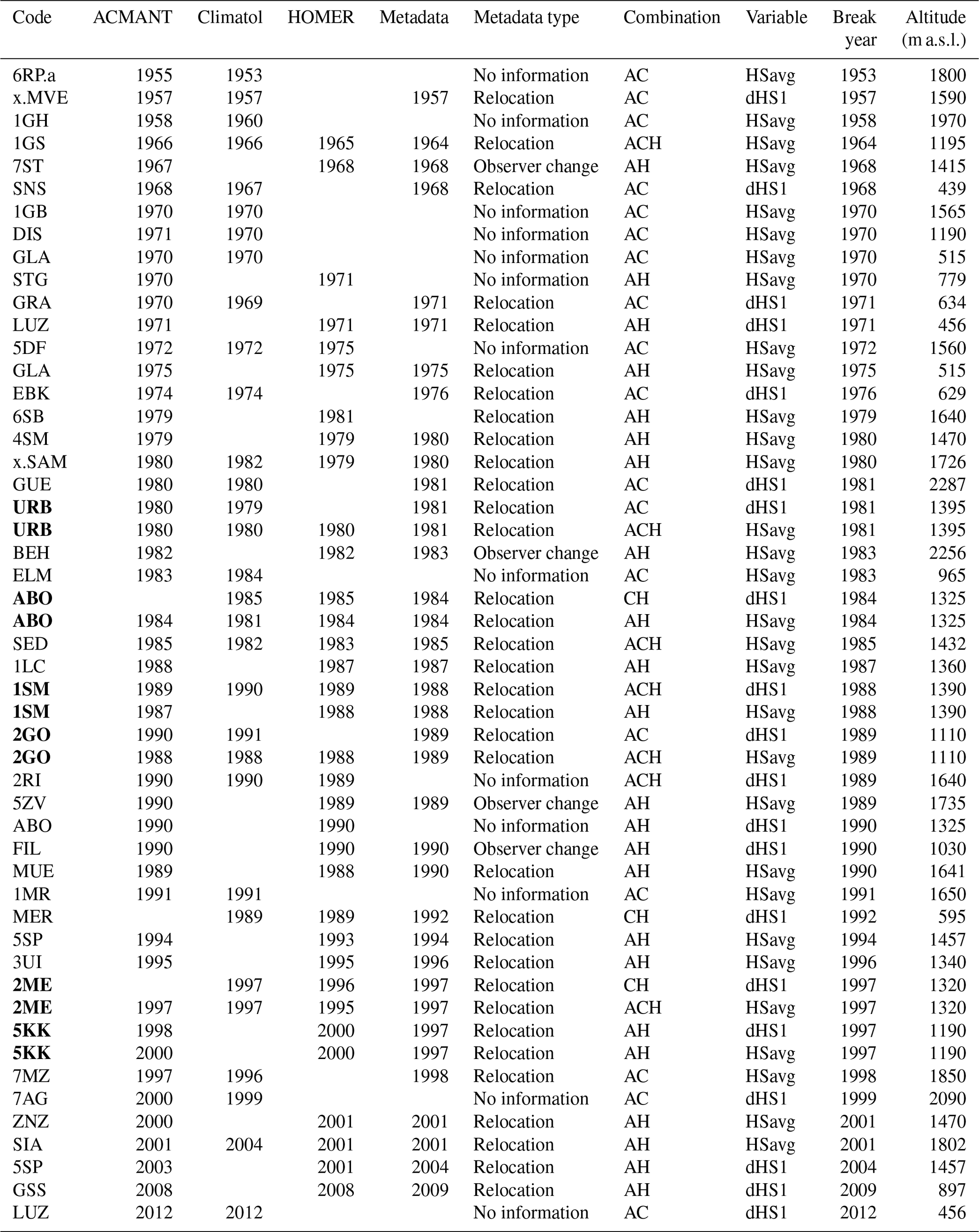
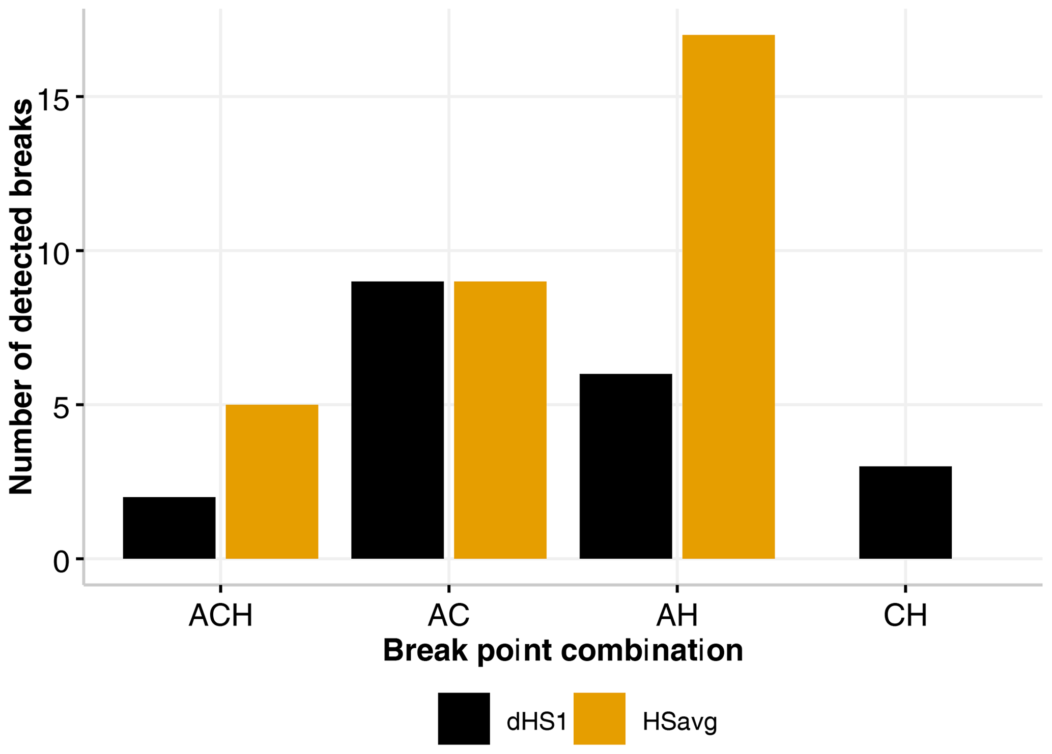
Figure 6 Method combinations for valid break points: ACMANT–Climatol–HOMER (ACH), ACMANT–Climatol (AC), ACMANT–HOMER (AH), and Climatol–HOMER (CH).

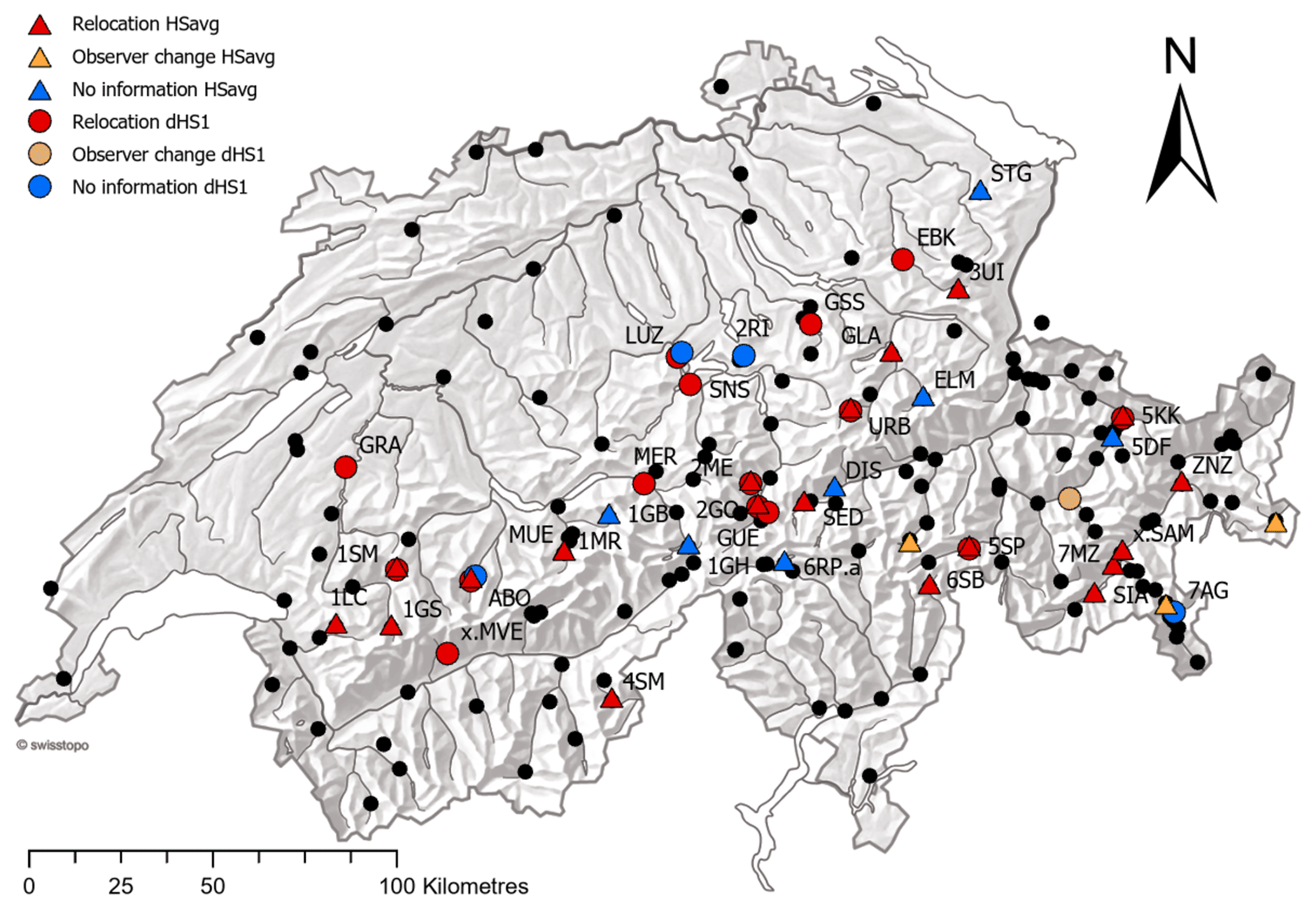
Figure 7 Map highlighting the location of series with identified valid break points and information from metadata where applicable. Series where no break points are detected are marked with black circles.

4.3 dHS1 as complementary information

The same procedures as outlined in Sect. 4.1 and 4.2 above were applied to another important and commonly used snow indicator: days with snow on the ground (dHS1). Here we found that for all methods except ACMANT, fewer break points are identified compared to the other measures (see Table 2). Here we found the majority of valid break points with the combination of ACMANT and Climatol (compared to AH for HSavg). From a total of 20 valid break points, ACMANT finds 17, followed by Climatol with 16 and HOMER with 11. This suggests that the dHS1 series appear to be more robust in terms of there being fewer breaks than for the HSavg series. Comparing the mean absolute break magnitude corrections for HSavg (14 %) with the ones for dHS1 (5 %) also reveals that the breaks identified in dHS1 are on average smaller than the ones found in HSavg. Table 2 (bottom) summarizes the number of identified breaks for the two indicators. Figure 8 compares the valid break points found for HSavg and dHS1. Six (out of 45) of the break points (13 %) agree, indicating that a complementary approach may be beneficial for detecting valid break points. Figure 7 provides an overview of the valid breaks and metadata information available for both HSavg and dHS1.

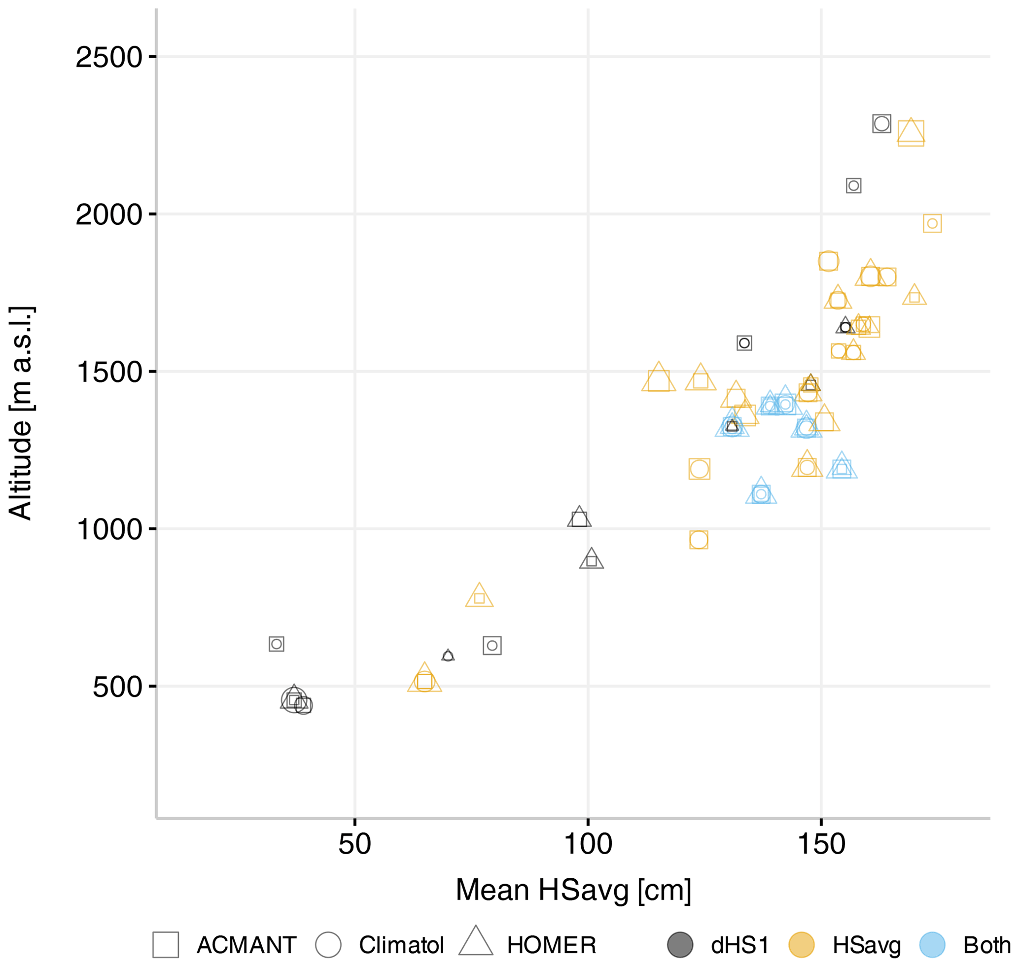
Figure 8 Comparison of valid break points found for HSavg and dHS1. Valid break points, detected by at least two methods, are coloured grey (dHS1), yellow (HSavg), or blue (both). The shape indicates which method detected the break, and the size is the corresponding break magnitude correction.

5 Discussions

5.1 Break detection

The main differences between the three methods arise from both the way reference series are constructed and how breaks are classified as valid. Reference series in ACMANT and HOMER are constructed based on correlation but with different correlation coefficient thresholds applied for the selection of reference series in the networks, whereas in Climatol, proximity (defined by Euclidean distances) is used. As these different configuration parameters allow for a large number of reference series combinations, as well as of ways breaks are classified, it is no surprise that the results differ between the methods. As the construction of reference series is an intrinsic part of the methods, a comparison with the same input network is not possible.

The detection capability of Climatol depends on the choice of wz (vertical scale parameter) and the SNHT thresholds as outlined by Guijarro (2018). However, the determination of appropriate SNHT thresholds is less straightforward, an issue which has been reported by Kuya et al. (2021a). Lowering the thresholds increased the number of identified break points. However, if the thresholds are too low, multiple breaks within the same years are detected, which implies that the method is too sensitive. Conversely, if the thresholds are too high, no breaks are detected at all. As suggested by Kuya et al. (2021a), the optimal threshold choice is one which prevents multiple break detections within the same year. The weight of the vertical coordinate (wz) is especially important for snow, as elevation in conjunction with small-scale topographic variation is an important control on snow depth.

ACMANT on account of its automation (and hence no user interaction) is the most objective method, but consequently there are no settings to optimize based on the judgement/experience of a practitioner (Pérez-Zanón et al., 2015). However, there seems to be a sensitivity issue with ACMANT: if using 188 instead of 184 series, the break points for some stations shifted slightly (±2 years) due to different station combinations being used as reference series. This indicates that the break detection algorithm is less robust or more dependent on available stations, especially as the correlation threshold used (0.4) is low. For comparison reasons, we did not perform any pre-treatment outside the actual methods (such as pre-defined neighbourhood networks); however, this might be beneficial for ACMANT (Domonkos and Coll, 2019).

Break detection in HOMER relies on multiple reference series in conjunction with support decisions from an experienced user. While this makes it the most robust application, it is also the most subjective of the three methods used here.

While there are many benchmark data sets for other climate variables (e.g. Willett et al., 2014; Venema et al., 2012), to date there are no such benchmarks for snow, which is unfortunate as these could have helped to thoroughly benchmark the methods. As the method with the highest number of detected breaks, ACMANT seems to be the most sensitive of the methods investigated here (Pérez-Zanón et al., 2015; Fioravanti et al., 2019), followed by Climatol and HOMER with smaller numbers of identified break points. Coll et al. (2020) found similar increments when analysing the break detection capabilities of ACMANT, Climatol, and HOMER for a large network of precipitation series in Ireland. Figure 5 shows no clear relationship between altitude, meanHSavg, and valid break points. Most valid break points are, however, detected at stations between 1000 and 1800 m a.s.l. A possible explanation for this is the large number of available stations in that particular elevation band, thereby ensuring that enough reference series are available. However, the network density for stations above 1800 m a.s.l. and below 1000 m a.s.l. is sparse by comparison, shown by Fig. 5. According to Gubler et al. (2017) the number of detected break points can be reduced by up to 50 % in sparse networks combined with a low signal-to-noise ratio (SNR).

Analysing the standard deviation of the ratio series (sigma, used as a proxy for noise) as well as the median correlations with HOMER reveals that for stations with altitudes below 800 and above 1800 m a.s.l., the range of the median sigma of the five reference series with the lowest sigma per candidate series is larger than for stations between 800 and 1800 m a.s.l. Figure S2 in the Supplement shows that relationship. A similar situation is clear when the median correlations of these subsets per candidate series are considered (Fig. S3). The higher noise (due to not enough suitable reference series being available) associated with these lower (and upper) stations may explain the different results between the networks at different densities and hence is a possible explanation for none of the methods detecting as many break points for stations in those elevation bands.

Break magnitude corrections

Break magnitude corrections and their corresponding density plots (Fig. 4) are similar to the ones found by Coll et al. (2020) working on Irish precipitation series. Differences in break magnitude corrections are also affected by different station neighbourhoods and arising from this the different subsets of stations used for the homogenization process. With a default internal correlation threshold of 0.4, ACMANT's neighbour selections cannot be the same as those of HOMER based on the 0.8 correlation threshold used.

5.2 Choice of method

According to our analyses, HOMER performs better than ACMANT or Climatol when the number of detected valid break points is compared to the number of break points detected overall. However, this comes at a cost based on the time input of the user and also requires extensive expert knowledge. In terms of ease of use based on automation, ACMANT would be the method of choice. However, sifting through the large number of break points detected involves a lot of post hoc processing and also requires in-depth knowledge about the network. Climatol provides the second-best efficiency (in terms of the ratio of valid breaks to total identified break points). However with 17 valid break points detected, 14 would have gone undetected without a combined approach; see Table 2. As outlined in Sect. 5.1 and reported by Kuya et al. (2021a), the results from Climatol heavily depend on the initial set-up. Coll et al. (2020) recommended Climatol as the method to use for precipitation because the identified break points appeared likely to be more realistic than the ones found with either ACMANT or HOMER in the analysis of their network. However, our analysis shows that this might not be the same when applied to snow series in a more topographically complex region. We found rather that a combination of the three methods works best and that HOMER performs significantly better than Climatol or ACMANT in the context of our network setting. This application of multiple methods was also used and recommended by Kuglitsch et al. (2012) and Toreti et al. (2012) for Swiss temperature series, as well as by Marcolini et al. (2019) for Austrian snow depth series. A recent study by Brugnara et al. (2020) applying homogenization methods to the phenological network in Switzerland also recommended this application of multiple methods.

Choice of variable – HSavg versus dHS1

Results from Buchmann et al. (2021b, a) concerning the stability, robustness, and variability in the snow variables HSavg and dHS1 investigated here suggest that HSavg is on average less stable and shows more variation than dHS1. The larger variability associated with HSavg when compared to dHS1 would be expected to lead to larger breaks and thus result in an increased likelihood of break point detection in HSavg. However, associated with these larger variations, there is also increased noise across the series, which has the effect of generally reducing the detection capability for lower-magnitude break points altogether. The variable dHS1, on the other hand, is more stable and shows less variability across the series, suggesting less noise for this variable and therefore break points with lower amplitudes overall. However, only looking at an average variability (or standard deviation) does not necessarily improve our understanding as the temporal evolution of variation of any single station is more important but is also a property affected by inhomogeneities. Analysing the mean absolute break magnitude corrections for the six break points identified in both HSavg and dHS1 reveals that the amplitudes of those detected for dHS1 are significantly smaller than the ones for HSavg. Break magnitude corrections retrieved from HOMER using breaks detected in dHS1 and inserted into HSavg do not differ from the ones obtained through breaks detected purely in HSavg. Based on this finding, break points detected in dHS1 may be used to calculate corrections for HSavg. These results tend to corroborate the hypothesis that the three methods detect smaller break points with dHS1 than with HSavg. For stations below 1000 m a.s.l. the majority of valid break points are detected in dHS1; hence these results tend to support the benefits of a complementary (dHS1 and HSavg) approach. As only six break points are identified with both variables, a complementary approach seems beneficial. Combining the results from both HSavg and dHS1 returns 45 (Table 2) valid break points in 184 Swiss snow time series.

5.3 Homogeneity of Swiss snow series

Our analysis shows the need for a combined use of some of the available methods in order to retrieve a set of break points for Switzerland where we can have higher confidence in their validity. In the majority of cases the methods agree well, with HOMER and Climatol returning the highest proportion of break points deemed valid based on the criteria we applied. Kuglitsch et al. (2012) could explain most of their break points for Swiss temperature series based on a combination of reasons, whereas our results tend to indicate that station relocation is the most likely source of inhomogeneities for the snow series analysed (Coll et al., 2020; Kuya et al., 2021a). However, due to the incomplete nature of the metadata available to support our study, we are unable to investigate this in more detail. For example, the entry “observer change” can mean change of observer only but may unfortunately also imply a combination of relocation and observer change. In spite of having identified relocation as the main explanation for the majority of break points, this is not consistently the case, since from a total of 519 recorded location changes in the station histories across the network, only 45 relocated stations (9 %) produced a valid break point across all three methods. The majority of our identified valid break points are located between 1000 and 1800 m a.s.l. at stations which normally experience continuous snow cover from November to April of the following year. From Fig. 7, the main geographical locations of series with breaks are the northern Prealps, Bernese Alps, and Engadine. The lack of inhomogeneity detections for series south of the Alps (Ticino) can largely be explained by a lack of suitable reference series available. The southern parts of Switzerland are dominated by low valleys surrounded by high mountains. This steep gradient in conjunction with small-scale varying climatic conditions seems to be a reason for not having enough reference series and subsequently inhibits any suitable break detection due to a lack of appropriate reference series.

Comparison with Italy, Austria, and the Alps

Similar break detection investigations have been performed for Italy, Austria, and the Austrian–Swiss domain: Marcolini et al. (2017) applied the SNHT to 106 closely adjacent snow time series for the same region of Italy, and in that work they reported 20 % of the series to be inhomogeneous. In terms of altitudinal and temporal extent, the data set used in that work is similar to ours; however, the 184 stations comprising our network are not from such a climatically coherent region.

Marcolini et al. (2019) investigated only 25 series between 200 and 1600 m a.s.l., whereas we analysed 184 series between 200 and 2500 m a.s.l. but only found valid break points in series between 500 (400 dHS1) and 2300 m a.s.l. (and the majority of these between 1000 and 1800 m a.s.l.). Moreover, Marcolini et al. (2019) found 11 (5 with the SNHT and PRODIGE) breaks in 25 series. They also reported an agreement of 45 % between the SNHT and PRODIGE in identifying the same break points. We only found 20 % (25 % for HSavg and 16 % for dHS1) agreement between Climatol and HOMER. In other work, Schöner et al. (2019) performed a break detection analysis on 96 Swiss snow series between 1961 and 2012 using PRODIGE and reported 25 series (26 %) as inhomogeneous. We found similar numbers: 17 % as inhomogeneous time series when only HSavg breaks are considered and 25 % with the complementary approach (HSavg and dHS1).

Using the complementary approach (HSavg and dHS1), we found similar numbers of potential break points to those that have been reported in previous studies (Marcolini et al., 2017, 2019; Schöner et al., 2019); this is in spite of the time periods and data sets used in our study not being identical. However, if we only compare the break points found in HSavg, our results show fewer break points than have been identified by the previous studies. Possible explanations for the differences are the combined use of three break detection methods in our work (rather than reliance on one method), as well as our fairly strict criteria for defining valid break points.

5.4 Further issues

The attribution of each valid break point to a single hydrological year is not straightforward, even when combined with the information from the available metadata, as not all series we defined as having valid break points had metadata available or, when metadata were available, they were not necessarily complete or entirely correct.

Furthermore, as the number and location of true break points in our data set remain unknown, statements about the probability of detection and false alarm rates (Brugnara et al., 2019) are not possible.

Stations below 500 m a.s.l. regularly experience winter months with little snow and only a few snow days; thus for a number of years in these records the recorded monthly means can be near zero. This lack of consistent snow records and the large variability (noise) associated with lower stations make it virtually impossible to have sufficient suitable reference series.

The next step to obtain homogenized snow series is to find the best method to use and further validate and subsequently correct the identified break points.

6 Conclusions

We present the first in-depth break point detection comparison of three homogenization methods for snow depth time series. In addition, we present the first detailed homogeneity assessment of Swiss snow depth series using state-of-the-art homogenization methods. Our analyses suggest that using ratios, working with monthly input data and annual detection, and combining the results from three methods (ACMANT, Climatol, HOMER) and two variables (HSavg and dHS1) offer a promising configuration to more accurately identify inhomogeneities in (Swiss) snow depth series.

Treating break points as valid when identified by at least two out of three methods and the application of strict criteria increase the robustness of, as well as the confidence in, the results compared to the use of a single method. For all the methods applied, expert knowledge about the network in question is indispensable. If, however, the practitioner is limited to only one method, based on the data and analysis here the method of choice would be HOMER. However, the approach combining multiple methods introduced here for application to snow depth series is more rigorous as it provides more confidence in the results. Concerning the total set of valid break points, ACMANT and Climatol appear to overestimate, whereas HOMER underestimates, the number of valid break points, for both HSavg and dHS1 based on the criteria used.

We identified 45 valid break points in 41 of 184 (22 %) series investigated using a complementary approach of HSavg and dHS1, of these 71 % could be explained by metadata, and based on the metadata, 88 % of the identified breaks could be attributed to station relocation. At low elevations, we identified a lack of suitable reference series due to many stations having inconsistent snow lie and being associated with large year-to-year variations, possibly masking the signal within the noise. However, further work is required, especially in view of the growing research effort in relation to attribution (break point verification) and homogenization (correction) efforts.