Towards ice-thickness inversion: an evaluation of global digital elevation models (DEMs) in the glacierized Tibetan Plateau

Accurate estimates of regional ice thickness, which are generally produced by ice-thickness inversion models, are crucial for assessments of available freshwater resources and sea level rise. A digital elevation model (DEM) derived from surface topography of glaciers is a primary data source for such models. However, the scarce in situ measurements of glacier surface elevation limit the evaluation of DEM uncertainty. Hence the influence of DEM uncertainty on ice-thickness modeling remains unclear over the glacierized area of the Tibetan Plateau (TP). Here, we examine the performance of six widely used and mainly global-scale DEMs: AW3D30 (ALOS – Advanced Land Observing Satellite – World 3D – 30 m; 30 m), SRTM-GL1 (Shuttle Radar Topography Mission Global 1 arc second; 30 m), NASADEM (NASA Digital Elevation Model; 30 m), TanDEM-X (TerraSAR-X add-on for Digital Elevation Measurement, synthetic-aperture radar; 90 m), SRTM v4.1 (Shuttle Radar Topography Mission; 90 m), and MERIT (Multi-Error-Removed Improved-Terrain; 90 m) over the glacierized TP by comparison with ICESat-2 (Ice, Cloud and land Elevation Satellite) laser altimetry data while considering the effects of glacier dynamics, terrain factors, and DEM misregistration. The results reveal NASADEM to be the best performer in vertical accuracy, with a small mean error (ME) of 0.9 m and a root mean squared error (RMSE) of 12.6 m, followed by AW3D30 (2.6 m ME and 11.3 m RMSE). TanDEM-X also performs well (0.1 m ME and 15.1 m RMSE) but suffers from serious errors and outliers on steep slopes. SRTM-based DEMs (SRTM-GL1, SRTM v4.1, and MERIT) (13.5–17.0 m RMSE) had an inferior performance to NASADEM. Errors in the six DEMs increase from the south-facing to the north-facing aspect and become larger with increasing slope. Misregistration of the six DEMs relative to the ICESat-2 footprint in most glacier areas is small (less than one grid spacing). In a next step, the influence of six DEMs on four ice-thickness inversion models – GlabTop2 (Glacier bed Topography), Open Global Glacier Model (OGGM), Huss–Farinotti (HF), and Ice Thickness Inversion Based on Velocity (ITIBOV) – is intercompared. The results show that GlabTop2 is sensitive to the accuracy of both elevation and slope, while OGGM and HF are less sensitive to DEM quality and resolution, and ITIBOV is the most sensitive to slope accuracy. NASADEM is the best choice for ice-thickness estimates over the whole TP.

1 Introduction

The Tibetan Plateau (TP), which includes the Pamir, Hindu Kush, Karakoram, Himalaya, and Tibet regions, covers an area of ∼3 000 000 km² and has a mean elevation of more than 4000 m a.s.l. (Fig. 1). It accounts for more than 82 % of the earth's land surface area above 4000 m a.s.l. (Fielding et al., 1994) and is often referred to as the Third Pole of the earth or the Asian Water Tower (Yao et al., 2012) due to its high elevation and abundant water resources in the form of glaciers, snow, permafrost, lakes, and rivers. The TP has a glacierized area of $\sim \mathrm{8.3}\times {\mathrm{10}}^{\mathrm{4}}$ km² (RGI Consortium, 2017) with an ice volume of $\sim \mathrm{6.2}\times {\mathrm{10}}^{\mathrm{3}}$ km³ (Farinotti et al., 2019), mainly distributed in the Karakoram and Himalaya regions.

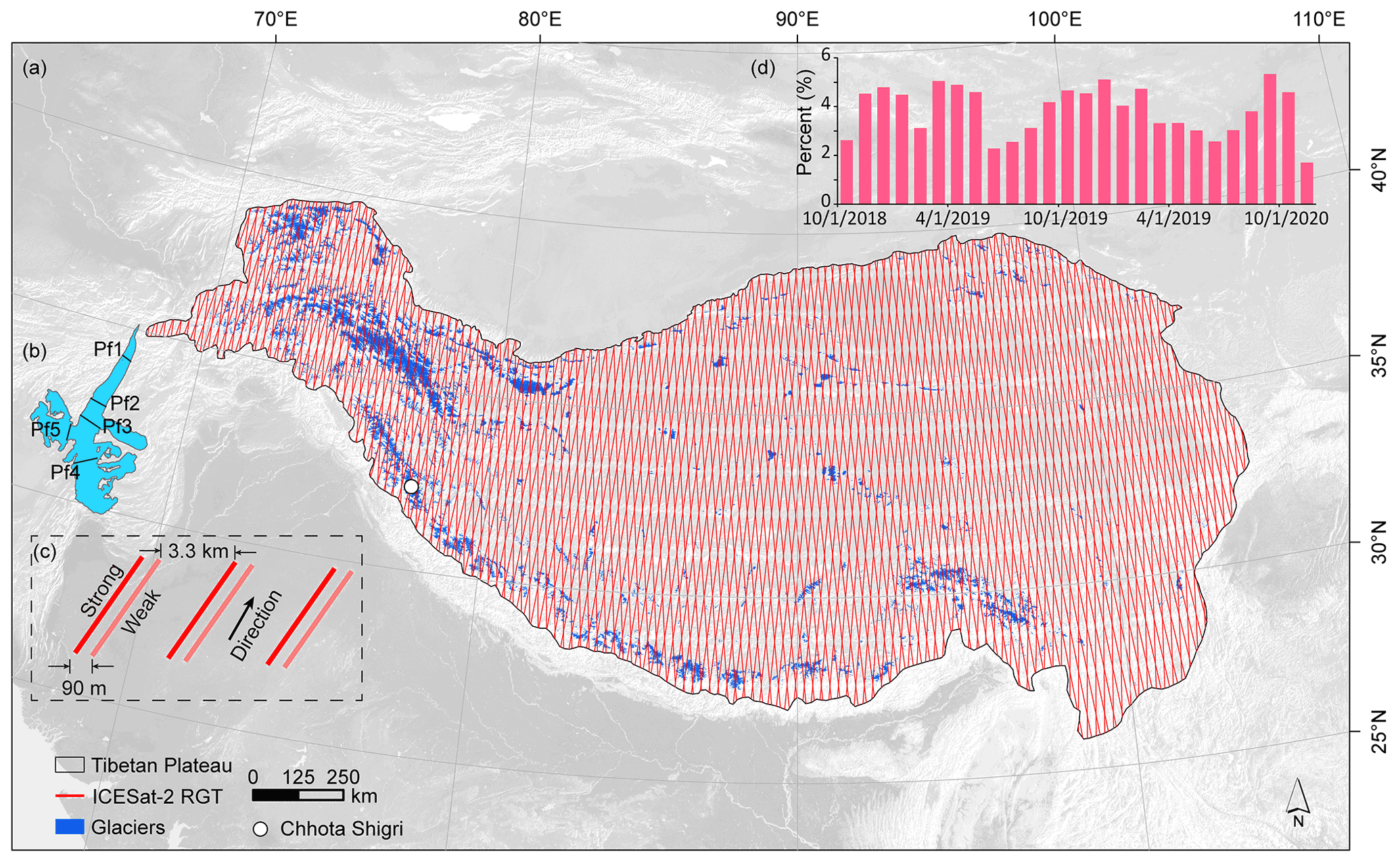
Figure 1 Location of the TP and its ICESat-2 (Ice, Cloud and land Elevation Satellite) reference ground tracks (RGTs). (a) ICESat-2 tracks over the TP and glaciers. (b) Location of ground-penetrating radar (GPR) profiles (Pf1–Pf5) over the Chhota Shigri Glacier which is used as an example (for location, see a). (c) Relative location of six beams when the Advanced Topographic Laser Altimeter System (ATLAS) has a backward orientation. The distance between RGTs is 28.8 km. (d) Percentage of ICESat-2 data in different months from October 2018 to November 2020. The boundary of the TP is derived from SRTM above 2500 m a.s.l. (Zhang et al., 2013).

Ice thickness is a crucial parameter for assessing the contribution of glaciers to global sea level rise (Kraaijenbrink et al., 2017), quantifying regional water availability (Huss and Hock, 2018; Immerzeel et al., 2020), and evaluating cryosphere-related hazards (Linsbauer et al., 2016; Zheng et al., 2021). In the TP, owing to the lack of in situ ice-thickness measurements (Welty et al., 2020), regional glacier thickness is mainly estimated by ice-thickness inversion models (ITIMs) using open-access digital elevation models (DEMs) (Farinotti et al., 2009, 2019; Frey et al., 2014). The DEM is a fundamental part of most regional ITIMs (Farinotti et al., 2017) and is often used to determine center flow lines (Maussion et al., 2019), shear stress (Frey et al., 2014; Wu et al., 2020), and apparent mass balance (Farinotti et al., 2009) and for ice-thickness interpolation (Huss and Farinotti, 2012). In addition to its use in ITIMs, the DEM has been an essential input for a wide range of TP glaciology studies, such as glacier inventory (Bhambri et al., 2011; Frey et al., 2012; Ke et al., 2016; Mölg et al., 2018), glacier mass change (Brun et al., 2017; Shean et al., 2020; Zhou et al., 2018), glacier-related disasters (Allen et al., 2019; Kääb et al., 2018; Zhang et al., 2019), and projections of glacier or glacial-lake evolution (Kaser et al., 2010; Kraaijenbrink et al., 2017; Zheng et al., 2021). The uncertainty in the DEMs can lead to different ITIM outcomes (Frey and Paul, 2012; Fujita et al., 2017; Furian et al., 2021; Kääb, 2005), especially for those ITIMs in which the DEM is a crucial input. For example, this includes the sensitivity of the Glacier bed Topography (GlabTop) model to slope increases for shallower slopes (Paul and Linsbauer, 2012), and an overestimation of slope by ∼10 % would result in an underestimation of ice thickness of ∼32 % (Linsbauer et al., 2012). Localized elevation errors and data gaps could affect the estimated ice thickness by 5 %–25 % using Huss–Farinotti model (Huss and Farinotti, 2012). Therefore, it is imperative to choose a suitable DEM source for regional glacier thickness modeling (Koldtoft et al., 2021). Farinotti et al. (2017, 2021) intercompare the performance of several ITIMs and suggest that consideration of the uncertainty in the input data could improve the model output. However, to our knowledge, the uncertainty in different open-access DEMs and their influence on various ITIM outputs over the TP have not been evaluated.

Currently, open-access DEMs covering the whole TP are mainly created by stereo mapping sensors such as ALOS AW3D30 (ALOS – Advanced Land Observing Satellite – World 3D – 30 m; Takaku et al., 2020), C- or X-band interferometry synthetic-aperture radar (InSAR) such as TanDEM-X (TerraSAR-X add-on for Digital Elevation Measurement), and SRTM-C-based (Shuttle Radar Topography Mission C-band) products such as NASADEM (NASA Digital Elevation Model; Crippen et al., 2016). Shadows and the layover effect of InSAR technology (González and Fernández, 2011), along with the deficient orientation of photogrammetrically stereo images (Mukherjee et al., 2013) or low stereo correlation (Hugonnet et al., 2021) propagated during DEM production, may introduce errors and voids. Filling these voids with other data could result in increased uncertainty (Liu et al., 2019). Additionally, the rugged terrain of glaciers and the low contrast of snow cover can often lead to geometric distortion and missing data (Reuter et al., 2007; Takaku et al., 2020). Estimates of the accuracy of DEMs in different terrains and landforms and for different vegetation coverage and land use have been conducted outside the TP using global navigation satellite system (GNSS) measurements or high-resolution DEMs (González-Moradas and Viveen, 2020; Grohmann, 2018; Hawker et al., 2019; Uuemaa et al., 2020). The performance of specific DEMs varied in these studies, indicating that the local terrain and land cover influenced the DEM accuracy. In the TP, glaciers are distributed across different climatic zones and have a wide range of elevations with rugged terrain (Fielding et al., 1994; Thompson et al., 2018). GNSS measurements are not accessible for most glaciers, and publicly available high-resolution DEMs are of lower quality due to their long temporal coverage (Shean, 2017). The assessment of DEM accuracy in specific regions with limited GNSS measurements or high-resolution DEMs is insufficient to determine the performance of global DEMs across the whole glacierized TP.

Liu et al. (2019) evaluated the performance of seven open-access DEMs over the TP with sparse Ice, Cloud and land Elevation Satellite (ICESat) altimetry data and suggested that AW3D30 has a high degree of accuracy. However, ICESat data with a footprint of 70 m (larger than the resolution of the estimated DEMs) could result in intra-pixel errors in steep slopes (Uuemaa et al., 2020). Besides, glacial regions were not considered in Liu et al. (2019), due to the variations of glaciers over time. Misregistration among DEMs, which may lead to evaluation bias (Han et al., 2021; Hugonnet et al., 2021; Van Niel et al., 2008), was also neglected. Bearing these issues in mind and considering the limitations of optics sensors in rugged terrain and the glacier accumulation area (Chen et al., 2021a), it is clear that a further assessment of the performance of AW3D30 over glacier areas is required. Recently, TanDEM-X (released in 2017) and NASADEM (released in 2020) have been reported to have large improvements in accuracy relative to previous DEM products for various land-cover types (Wessel et al., 2018), floodplain sites (Hawker et al., 2019), slightly undulating terrain (Altunel, 2019), and mountain environments (Gdulová et al., 2020). Nonetheless, their performance over the rugged and glacierized TP remains unclear.

The purpose of this study is to evaluate the optimal DEM to use for regional ice-thickness estimation over the TP. We first evaluated the performance of six widely used DEMs – AW3D30, SRTM-GL1 (Shuttle Radar Topography Mission Global 1 arc second), NASADEM, TanDEM-X, SRTM v4.1, and MERIT (Multi-Error-Removed Improved-Terrain), which are derived from different sensors and have different resolutions – against ICESat-2 data which have been proven to have high vertical accuracy and resolution (Brunt et al., 2019, 2021; Li et al., 2021) but with sparse tracks (Fig. 1). The elevation differences between these DEMs and ICESat-2 are systematically analyzed concerning aspect, slope, elevation, and glacier zones. The influence on the accuracy assessment from the glacier elevation changes, terrain, and misregistration among DEMs is then quantified. Finally, we compare the performance of ice thickness modeled by using the six DEMs against in situ measurements of ice thickness by ground-penetrating radar (GPR).

2 Data and methods

2.1 ICESat-2 elevation data

ICESat-2, a follow-on mission to ICESat, was launched on 15 September 2018, with the goal of acquiring the earth's geolocated surface elevation referenced to the WGS84 ellipsoid at the photon level. ICESat-2's ATLAS (Advanced Topographic Laser Altimeter System) emits a pulse every 0.7 m along the track covering a horizontal circular area with 0.5 m in vertical extent and ∼17 m in diameter. This design diameter value varied due to the photo-counting lidar technology and potentially the atmospheric conditions (Magruder et al., 2020). ICESat-2's ATL03 and ATL06 products can both be used as an elevation reference. The ATL03 product has a spacing of ∼0.7 m and can provide more terrain details than the ATL06 product. In this study, based on the resolution of global DEM and computational cost, we select the ICESat-2 Level-3A land-ice ATL06 product as an elevation reference. ATL06 heights are median-based heights derived from a linear-fit model over each segment corrected for first-photon bias and transmit-pulse shape. The segment has a length of 40 m centered on reference points at 20 m intervals along the track. The ATL06 product has better than 5 cm height accuracy and better than 20 cm surface measurement precision in the Antarctic (Brunt et al., 2019, 2021; Li et al., 2021) and Qilian Shan (Zhang et al., 2020). The product also contains land background points. The RGI 6.0 (Randolph Glacier Inventory) glacier inventory (RGI Consortium, 2017) was used to extract points falling on glaciers (Fig. 2).

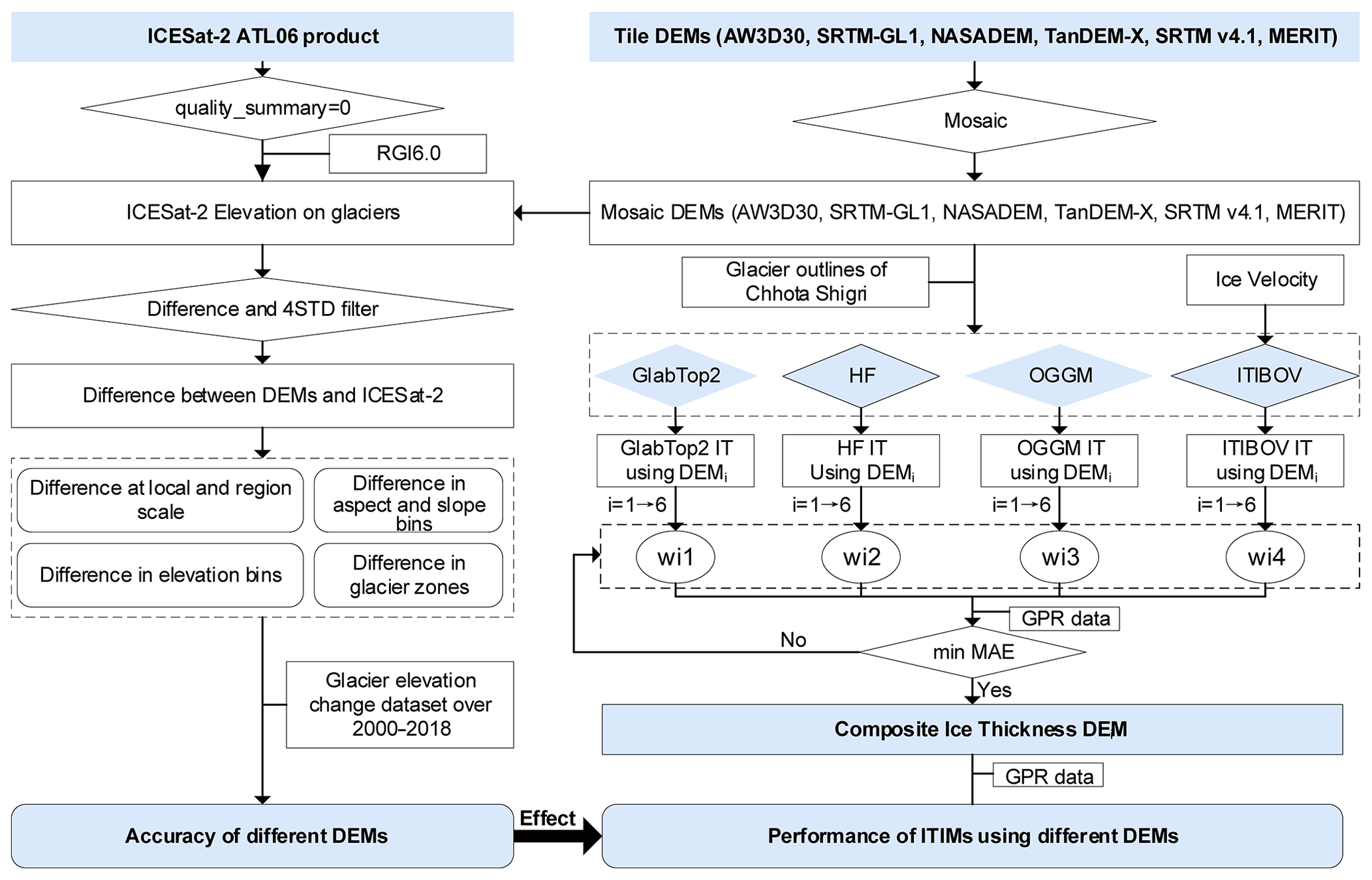
Figure 2 Flow chart showing the targets and methods used in this study including an accuracy evaluation of DEMs and their effects on ice-thickness inversion models. The abbreviations wi1, wi2, wi3, and wi4 denote the weight of each modeled ice thickness; i from 1 to 6 denotes six different DEMs; and the number 1–4 denotes the four ice-thickness inversion models. 4STD: 4 standard deviations. IT: ice thickness.

ICESat-2 ATL06 data covering the TP from October 2018 to November 2020 were downloaded from https://earthdata.nasa.gov/ (last access: 5 March 2021) (Fig. 1). There are 2436 files containing about 100 GB of data in total. The fields location (latitude, longitude), surface elevation (h_li), elevation uncertainty (h_li_sigma), and quality (atl06_quality_summary) were used. By combining the quality field (atl06_quality_summary = 0) (Smith et al., 2019) with the glacier inventory, a total of 3.5 million points out of 0.16 billion records over the TP were selected (Fig. 1). The slope, aspect, and elevation value of the cell center of the DEMs were extracted for the ICESat-2 footprints.

2.2 Global DEMs

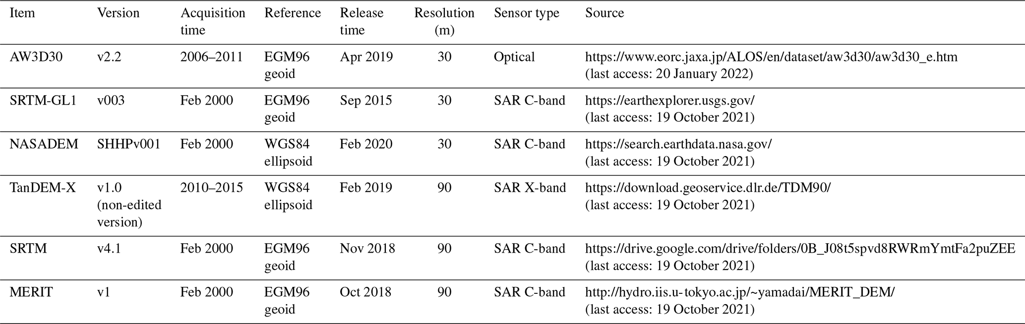
Six global-scale DEMs were selected for the evaluation of ITIM sensitivity, based on popularity, data source, resolution, and sensor type (Table 1).

1. ALOS World 3D – 30 m (AW3D30) is acquired by the optics stereo sensor loaded on the Advanced Land Observing Satellite (ALOS) which operated from 2006 to 2011 with a horizontal resolution of 30 m. Approximately 10 % of global land area, mainly in tropical rainforest areas and the polar areas, has voids mostly due to cloud or snow/ice cover constatation in source imageries. Data gaps are filled with SRTM, ASTER GDEM v3 (Advanced Spaceborne Thermal Emission and Reflection Radiometer Global Digital Elevation Model), ArcticDEM v3, and TanDEM-X 90 (Takaku et al., 2020). After filling gaps, the accuracies in void-filled and void-free areas are nearly consistent (Takaku et al., 2020). Data were available at https://www.eorc.jaxa.jp/ALOS/en/dataset/aw3d30/aw3d30_e.htm (last access: 20 January 2022) after user registration.

2. TanDEM-X 90 m DEM (hereafter TanDEM-X) is a product derived from the first bistatic X band SAR mission of the world which took place from 2014 to 2016 (Bachmann et al., 2021). It is a pixel-reduced product of the global TanDEM-X DEM with a grid spacing of 0.4 arcsec (12 m). The official reported absolute vertical and horizontal accuracy is better than 10 m at the 90 % confidence level. It is noted that the current release is a non-edited version: areas with outliers, noise, and voids remain. The original data were collected during different seasons and years, inducing errors due to (seasonal and long-term) accumulation/ablation on glaciers. Data were acquired from https://download.geoservice.dlr.de/TDM90/ (last access: 19 October 2021).

3. NASADEM is a new product released in 2020, which is derived by reprocessing the original SRTM signal data using updated interferometric unwrapping algorithms and auxiliary data, such as ICESat, to reduce voids and improve vertical accuracy (Crippen et al., 2016). Remnant voids are filled mainly by Global Digital Elevation Model (GDEM) v3 data. These data were downloaded from https://search.earthdata.nasa.gov/ (last access: 19 October 2021).

4. SRTM-GL1 (30 m) is an extensively used DEM in ITIMs. Voids were primarily filled by ASTER GDEM2.

5. SRTM v4.1, with a spatial resolution of 90 m, is produced by the method proposed by Reuter et al. (2007), including merging tiles, filling small holes iteratively, and interpolating across the holes using a range of methods, according to the size of the hole and the land type surrounding it (https://cgiarcsi.community/data/srtm-90m-digital-elevation-database-v4-1/, last access: 19 October 2021). SRTM v4.1 was also used to compare against the performance of SRTM-GL1 to estimate the influence of resolution. The first open-access ice-thickness database of global glaciers also adopted SRTM v4.1 as its DEM source (Farinotti et al., 2019).

6. MERIT is also widely used with a spatial resolution of 90 m. It was developed by removing absolute bias, stripe noise, speckle noise, and tree height bias from the existing spaceborne DEMs (SRTM3 v2.1 and AW3D30 v1) using multiple satellite datasets and filtering techniques (Yamazaki et al., 2017). Its accuracy was significantly improved, especially in flat regions (Yamazaki et al., 2017). The overall accuracy is similar to TanDEM-X in floodplain sites (Hawker et al., 2019) but lower in short vegetation. The dataset was downloaded from http://hydro.iis.u-tokyo.ac.jp/~yamadai/MERIT_DEM/ (last access: 19 October 2021). SRTM v4.1 and MERIT were selected to compare with TanDEM-X and simultaneously estimate the influence of DEM resolution on ITIMs.

Elevations of ICESat-2 data, NASADEM_SHHPv001, and TanDEM-X are based on a WGS84 ellipsoid reference and elevations of the other four DEMs are based on an EGM96 geoid (Table 1). The function of geoidheight provided by MATLAB was used to calculate geoid height to unify their references.

Table 1 Details of the selected DEMs.

2.3 Ice-thickness inversion methods

Tiles of six DEMs (AW3D30, TanDEM-X, NASADEM, SRTM-GL1, SRTM v4.1, and MERIT) were used to form a mosaic of terrain data covering the whole TP. Four ice-thickness inversion models (GlabTop2, Glacier bed Topography; HF, Huss–Farinotti; OGGM, Open Global Glacier Model; and ITIBOV, Ice Thickness Inversion Based on Velocity) were used to estimate the glacier thickness. The Chhota Shigri Glacier located in the western Himalaya with available GPR data (Fig. 1) was selected as an example to evaluate the influence of DEM uncertainty on the ITIMs. The GPR data were measured based on a pulse radar system in October 2009 (Azam et al., 2012) and is available at Farinotti et al. (2021). Full details of the ITIMs are given below.

GlabTop (Glacier bed topography) is based on the theory that glacier thickness is mainly determined by the slope of the terrain (Linsbauer et al., 2012; Paul and Linsbauer, 2012). It is assumed that the glacier is an ideal plastic fluid, with basal slip being ignored. Based on the empirical relationship between mean shear stress along the center lines and the range of glacier elevation (Haeberli and Hoelzle, 1995) (Eq. 1), the actual basal shear stress τ can be determined.

$$\begin{array}{}\text{(1)}& \begin{array}{rl}& \mathit{\tau }=\mathrm{0.005}+\mathrm{1.598}\mathrm{\Delta }H-\mathrm{0.435}\mathrm{\Delta }{H}^{\mathrm{2}}\\ & \mathit{\tau }=\mathrm{150}\mathrm{kPa},\mathrm{if}\mathrm{\Delta }H>\mathrm{1600},\end{array}\end{array}$$

where ΔH is the elevation range of the glacier. The ice thickness h can then be determined from Eq. (2)

$$\begin{array}{}\text{(2)}& h={\displaystyle \frac{\mathit{\tau }}{f\mathit{\rho }g\sin \mathit{\alpha }}},\end{array}$$

where f is the shape factor, ρ is glacier density (850±60 kg m⁻³) (Huss, 2013), g is the acceleration due to gravity (9.8 m s⁻²), and α is the slope. GlabTop2 is an automated method for calculating ice thickness similar to GlabTop but avoids digitizing the branch lines. For details refer to Frey et al. (2014).

The HF (Huss–Farinotti) model is based on the mass balance principle which relates the surface mass balance of the glacier (b) to the ice flux and variation in the glacier thickness. Given the ice flux, ice thickness can be calculated according to Glen's ice flow law (Farinotti et al., 2009; Huss and Farinotti, 2012).

$$\begin{array}{}\text{(3)}& h=\sqrt[n+\mathrm{2}]{{\displaystyle \frac{q(\mathrm{1}-\mathrm{fsl})}{\mathrm{2}A}}{\displaystyle \frac{n+\mathrm{2}}{(f\mathit{\rho }g\sin \mathit{\alpha }{)}^n}}},\end{array}$$

where h is the mean elevation of band thickness, q is the ice flux, fsl=0.8 is the basal-slip correction factor, n=3 is the exponent of flow law, ρ is glacier density (850±60 kg m⁻³), g is the acceleration due to gravity (9.8 m s⁻²), f=0.8 is the valley shape factor (Cuffey and Paterson, 2010), and A is the Glen flow rate factor (3.24×10²⁴ Pa⁻³ s⁻¹) (Cuffey and Paterson, 2010; Gantayat et al., 2014).

This method defines a new variable, $\stackrel{\mathrm{̃}}{b}=\dot{b}-\mathit{\rho }g\frac{\partial h}{\partial t}$, where $\stackrel{\mathrm{̃}}{b}$ is the apparent mass balance, $\dot{b}$ is the glacier surface mass balance, and $\frac{\partial h}{\partial t}$ is the glacier surface elevation change. $\stackrel{\mathrm{̃}}{b}$ is linearly related to the elevation. In the absence of mass balance data and thickness change data on the surface of a glacier, the ice flux q can be obtained by estimating $\stackrel{\mathrm{̃}}{b}$, which is determined from Huss and Farinotti (2012). Ice thickness in each elevation band can then be determined by substitution into Eq. (3). Finally, h is extrapolated, in combination with the slope, to obtain the distributed ice thickness, according to the parameters in Huss and Farinotti (2012).

The Open Global Glacier Model (OGGM) is based on the same concept as HF but has two main differences (Maussion et al., 2019). Firstly, the method described in Kienholz et al. (2014) is used to automatically obtain the middle streamlines and watershed division. Secondly, the apparent mass balance data are reconstructed from the local climatic dataset from variables such as precipitation and temperature.

The Ice Thickness Inversion Based on Velocity (ITIBOV) model is inverted from the shallow ice approximation; it obtains the ice thickness by combining the surface velocity field with the Glen ice flow law (Gantayat et al., 2014; Glen, 1955):

$$\begin{array}{}\text{(4)}& h={\displaystyle \frac{n+\mathrm{1}}{\mathrm{2}A}}{\displaystyle \frac{(\mathrm{1}-k)u_{\mathrm{s}}}{(f\mathit{\rho }g\sin \mathit{\alpha }{)}^n}},\end{array}$$

where h is ice thickness, u_s is glacier surface velocity, and k is the contribution ratio of basal-slip velocity relative to u_s. We used the mean velocity over 1985–2019 from the ITS_LIVE dataset (Inter-mission Time Series of Land Ice Velocity and Elevation; Gardner, 2019) as the u_s input. We assumed that basal slip only occurred during the warm seasons, and k was calculated by dividing the annual glacier velocity by winter glacier velocity (Wu et al., 2020). Data from the Global Land Ice Velocity Extraction from Landsat 8 (GoLIVE) dataset with a date separation length of fewer than 96 d are used to estimate the monthly velocity (Fahnestock et al., 2016; Scambos, 2016), allowing the winter velocity (December, January, and February) and annual mean velocity to be calculated. Basal factor k was calculated as 0.80 (Fig. S1 in the Supplement). The shared parameters, such as creep factor, shape factor, and basal creep factor are same in all four models.

An ensemble of the output from different models can improve the modeled thickness (Farinotti et al., 2017, 2021). Therefore, after calculating the ice thickness from four models using different DEMs, we calculated an ensemble ice thickness using the same DEM but with different models. First, the ensemble ice thickness was the sum of the four models with weights w1, w2, w3, and w4, respectively. The sum of four weights equals 1: 70 % of the GPR data are adopted as calibration data, and 30 % of the GPR results are adopted as validation data. Then, the four weights are iteratively changed to achieve the minimal mean absolute error between calibration data and the model result. Finally, the mean absolute error (MAE) between ensemble ice thickness and validation data are calculated.

2.4 Accuracy assessment method

The error in the DEMs is considered to be the difference between the DEM elevation and the ICESat-2 measurements. To remove the influence of outliers, elevation differences greater than 4 standard deviations were removed. Mean error (ME), MAE, median error, root mean square error (RMSE), standard deviation (SD), and normalized median absolute deviation (NMAD) were calculated for the error analysis. NMAD and ME were used to assess the disturbance from extreme errors (Höhle and Höhle, 2009; Gdulová et al., 2020). When calculating the ME, the positive and negative biases cancel each other, making the error smaller; therefore, the SD together with ME could be a complementary indicator for assessment.

$$\begin{array}{}\text{(5)}& {\displaystyle }& {\displaystyle }\mathrm{ME}={\displaystyle \frac{\mathrm{1}}{n}}\sum _{\mathrm{1}}^n\left(H_{\mathrm{DEM}}-H_{\mathrm{ICESat}\text{-}\mathrm{2}}\right),\text{(6)}& {\displaystyle }& {\displaystyle }\mathrm{MAE}={\displaystyle \frac{\mathrm{1}}{n}}\sum _{\mathrm{1}}^n\mathrm{abs}\left(H_{\mathrm{ICESat}\text{-}\mathrm{2}}-H_{\mathrm{DEM}}\right),\text{(7)}& {\displaystyle }& {\displaystyle }\mathrm{RMSE}=\sqrt{{\displaystyle \frac{\mathrm{1}}{n}}\sum _{\mathrm{1}}^n{\left(H_{\mathrm{ICESat}\text{-}\mathrm{2}}-H_{\mathrm{DEM}}\right)}^{\mathrm{2}}},\text{(8)}& {\displaystyle }& {\displaystyle }\mathrm{SD}=\sqrt{{\displaystyle \frac{\mathrm{1}}{n-\mathrm{1}}}\sum _{\mathrm{1}}^n{\left(H_{\mathrm{ICESat}\text{-}\mathrm{2}}-H_{\mathrm{DEM}}-\mathrm{ME}\right)}^{\mathrm{2}}},\text{(9)}& {\displaystyle }& {\displaystyle }\mathrm{NMAD}=\mathrm{1.4826}\cdot \mathrm{median}\left(\mathrm{abs}\left(H_{\mathrm{ICESat}\text{-}\mathrm{2}}-H_{\mathrm{DEM}}\right)\right),\end{array}$$

Glacier surface elevation change ranged between −21 and 17 m yr⁻¹ over the TP during 2000–2018 (Shean et al., 2020). Therefore, the disparity of acquisition date between ICESat-2 and six DEMs (Table 1) could introduce large errors due to the changing glacier geometry. This applies in particular to TanDEM-X and AW3D30, which are collected in different months and years (Table 1). However, the other four DEMs are produced from NASA's Shuttle Radar Topography Mission during the 11 d mission in February 2000. We selected ICESat-2 data acquired in February 2019 and 2020. Then the glacier elevation dynamic magnitude between February 2000 and February 2019 or February 2020 (Shean et al., 2020) is subtracted from the selected ICESat-2 elevation. By comparing the elevation differences from the adjusted ICESat-2 data and the four DEMs, we could partly estimate the impacts of glacier dynamics on accuracy assessment.

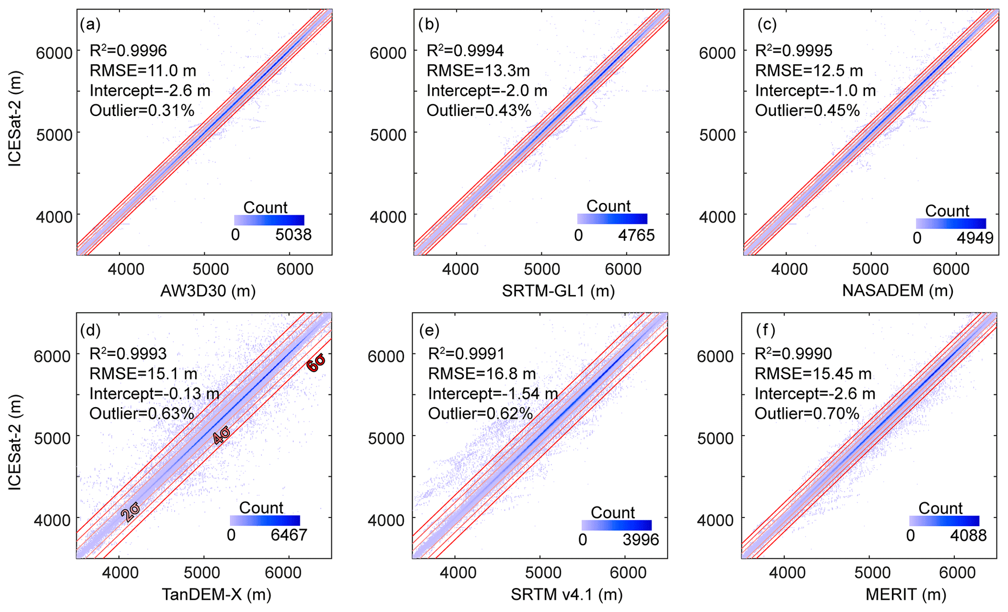
Figure 3 Differences between six DEMs and ICESat-2 elevation. (a) AW3D30, (b) SRTM-GL1, (c) NASADEM, (d) TanDEM-X, (e) SRTM v4.1, and (f) MERIT. The gradually lighter red lines in (d) denote the range within 6, 4, and 2σ of the mean. The text at the top left of each panel gives the fit results for data within 4σ of the mean. Outlier denotes the proportion of outliers relative to the total records. R², RMSE, and intercept are fit results when the slope coefficient is set to 1. The elevation range was cut to 3500–6500 m a.s.l., the range in which most elevations values are located, to show clearly the effect of using different multiples of the SD from the mean.

3 Results

3.1 Accuracy of DEMs

The level of 4 standard deviations (that is 4σ) was chosen to not only filter the differences between ICESat-2 and DEMs to exclude extreme outliers but also keep most records in the further accuracy analysis. The ratio of excluded outliers relative to the record of each DEM is less than 1 %. Overall, there is no irregular deviation among these DEMs and ICESat-2 elevation after filtering (Fig. 3). The ICESat-2 vs. DEMs values are distributed tightly around the fit line with a slope coefficient of 1, with no obvious differences among the R². NASADEM and TanDEM-X performed the best in terms of intercept and fit RMSE, with very little difference to the ICESat-2 data.

Statistically, the median and ME did not differ much, which indicated that extreme values did not influence the ME much after the filter of 4 standard deviations was applied (Fig. 4). SD was slightly larger than NMAD, especially for TanDEM-X, indicating larger discrepancies due to the DEM errors and noise (Höhle and Höhle, 2009). NASADEM performed better than the other two 30 m resolution DEMs in ME. AW3D30 behaved best in RMSE (11.3 m) and MAE (8.2 m). SRTM-GL1 and NASADEM are both produced from the same original SAR data but differ in RMSE (13.5 m vs. 12.6 m), MAE (10.0 m vs. 9.4 m), and ME (2.0 m vs. 0.9 m). The new algorithm and auxiliary data applied in NASADEM do indeed improve the absolute accuracy of the product over glacierized terrain. The quality of TanDEM-X was the best out of the 90 m resolution DEMs with the smallest RMSE (15.1 m), MAE (8.9 m), ME (0.1 m), and SD (15.1 m). SRTM v4.1 and MERIT are both error-reduced products from SRTM3 v2 (Reuter et al., 2007; Yamazaki et al., 2017), and they have similar ME (−1.5 m vs. 2.6 m) and RMSE (17.0 m vs. 15.6 m).

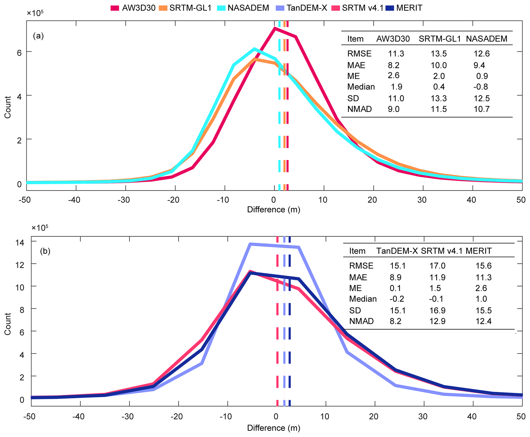
Figure 4 Overall difference (m) statistics between six DEMs and ICESat-2 elevation: (a) 30 m resolution DEMs – AW3D30, SRTM-GL1, and NASADEM – and (b) 90 m resolution DEMs – TanDEM-X, SRTM v4.1, and MERIT. The vertical dashed lines denote the mean elevation difference of each DEM between ICESat-2. ME is mean error; MAE is mean absolute error; median is median error; RMSE is root mean square error; SD is standard deviation; and NMAD is normalized median absolute deviation.

Spatially, the ME in southeast Tibet is more positive than that in the Himalaya, and it is slightly negative in the western Kunlun and Karakoram (Fig. 5a). It is worth noting that in the Himalaya and southeast Tibet, the ME of the other four DEMs is more positive than that of TanDEM-X and AW3D30. ME of TanDEM-X are mainly at ±5 m but with some large values in several regions. SRTM-GL1, NASADEM, SRTM v4.1, and MERIT have nearly the same distribution of ME and show negative ME values in the western Kunlun and Karakoram. The ME of NASADEM is smaller than that of SRTM-GL1 in most regions of the TP but is bigger in the western Kunlun and Karakoram. Overall, the SD of 30 m resolution DEMs is much better than that of 90 m resolution DEMs (Fig. 5b). The SD along the Hindu Kush–Himalaya and southeast Tibet was larger than that in other regions. The SD in southeast Tibet was relatively larger (>12 m). Specifically, the SDs of AW3D30 and NASADEM were the smallest and shared similar spatial distribution features. The SD of NASADEM was improved over most parts of the TP, compared with that of SRTM-GL1 (Fig. 5b). This indicates that some disturbances from noise and errors may exist in SRTM-GL1, SRTM v4.1, and MERIT in the western Kunlun and Karakoram. TanDEM-X performs well in overall statistics (Fig. 4b) and ME (Fig. 5a) but did not show large improvements in SD and was even worse in some areas. The SD and ME of SRTM v4.1 and MERIT have the same spatial distribution (Fig. 5b) and have similar overall SD (both ∼15 m) and ME (both ∼2 m) values (Fig. 4b).

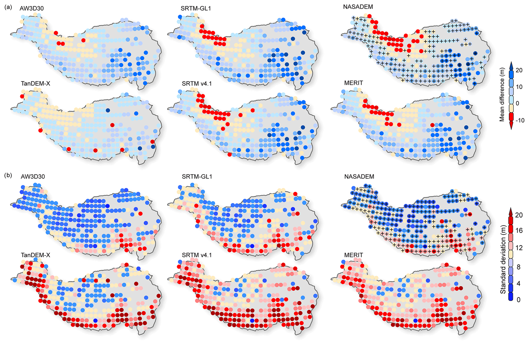
Figure 5 Aggregated spatial mean error (ME) (a) and standard deviation (SD) (b) between six DEMs and ICESat-2 elevation for $\mathrm{1}{}^{\circ }\times \mathrm{1}{}^{\circ }$ cells across the TP. The cross symbol denotes that NASADEM performs better than SRTM-GL1 in ME or SD.

3.2 Differences between DEMs and ICESat-2 in aspect, slope, and elevation

The influence of aspect is most apparent for SRTM-GL1, with a median value of about −5 m in the south aspect, which increased in magnitude gradually towards to the north aspect (∼5 m). A similar pattern but with a smaller amplitude is found for NASADEM, TanDEM-X, MERIT (−1 to 1 m), and AW3D30 (0 to 2 m) (Fig. 6a).

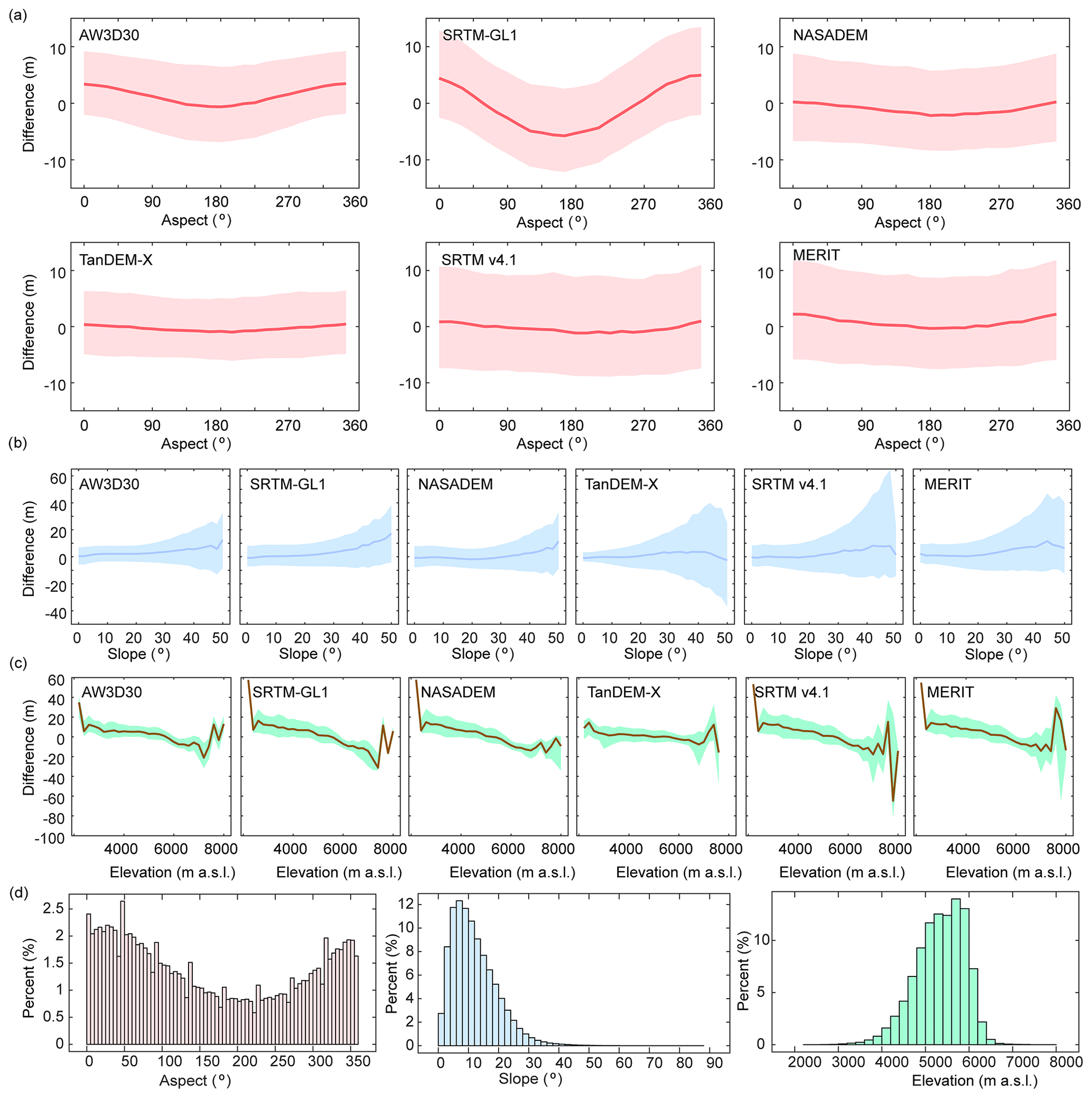
Figure 6 Differences between six DEMs and ICESat-2 with terrain factors: (a) 5^∘ aspect bin; (b) 2^∘ slope bin; (c) 200 m elevation bin; and (d) percentage (%) of data in each aspect, slope, and elevation bin.

The median differences of the 30 m DEMs generally increased along the slope. However, for the 90 m DEMs, the difference increased with slope at first but then decreased on steep slopes. NASADEM and TanDEM-X had minimum mean median values of about 0.9 and 1.2 m, respectively (Fig. 6b). For all DEMs, the spread of difference becomes larger as the slope becomes steeper. This increase is most obvious for TanDEM-X and SRTM v4.1, with rates of 1.29 m per degree (r=0.97, p<0.01) and 1.11 m per degree (r=0.89, p<0.01). This indicated that errors of both DEMs suffered from steep slope effects. AW3D30 and NASADEM have a similar mean spread (19.2 m vs. 20.8 m). On slopes of less than 20^∘, TanDEM-X has the best quality with a mean median value of −0.2 m and mean spread of 11.7 m, respectively. MERIT shows a slight advantage over SRTM v4.1 with a reduced spread for steep slopes. Overall, relative to the other DEMs, AW3D30 and NASADEM perform best for steep slopes in terms of spread and median value.

The differences for all DEMs generally decreased with elevation, with fluctuations around zero at very high elevations (Fig. 6c). AW3D30 has a smaller difference at low elevation relative to NASADEM and SRTM-GL1. For NASADEM and SRTM-GL1, the differences along the elevations show a similar distribution and varied from −10 to 10 m over the range 4500–6500 m a.s.l., where measurements are concentrated (Fig. 6d). However, NASADEM behaves best out of the six DEMs at high elevation. The difference of TanDEM-X varied from around −5 to 5 m between 4500 and 6500 m a.s.l. The SRTM v4.1 and MERIT differences changed almost similarly from −20 to 40 m but show differences at the highest elevations.

3.3 Differences between DEMs and ICESat-2 in different glacier zones

Elevation differences in different glacier zones were also estimated and are shown in Fig. 7a–d. We divided it into four sub-zones using the maximum, median, and minimum elevation from the RGI glacier inventory (Fig. 7e). Here we consider Zone 1 and Zone 4 to be the ablation area and accumulation area, respectively. Zone 2 and Zone 3 are transition areas. Crests of the probability distribution of differences located in the positive axis range in Fig. 7a move to the left in Fig. 7b–d. Correspondingly, ME, MAE, and RMSE all decrease from Zone 1 (ablation area) to Zone 2 (transition area) (Fig. 7 and Table S1 in the Supplement). Spatially, areas in the glacier terminus are subject to more melting (Brun et al., 2017), leading to this decrease. The ME of the SRTM-based products SRTM-GL1, SRTM v4.1, NASADEM, and MERIT are all around 10 m in Zone 1 and decreased similarly by 8.1, 7.6, 7.5, and 7.2 m towards Zone 2, respectively (Table S1). Temporally, the ME of the DEM acquired in earlier periods is bigger. The ME is 8.1 m for AW3D30, which was acquired in 2006–2011, bigger than that of TanDEM-X (3.9 m), which was acquired in 2010–2015.

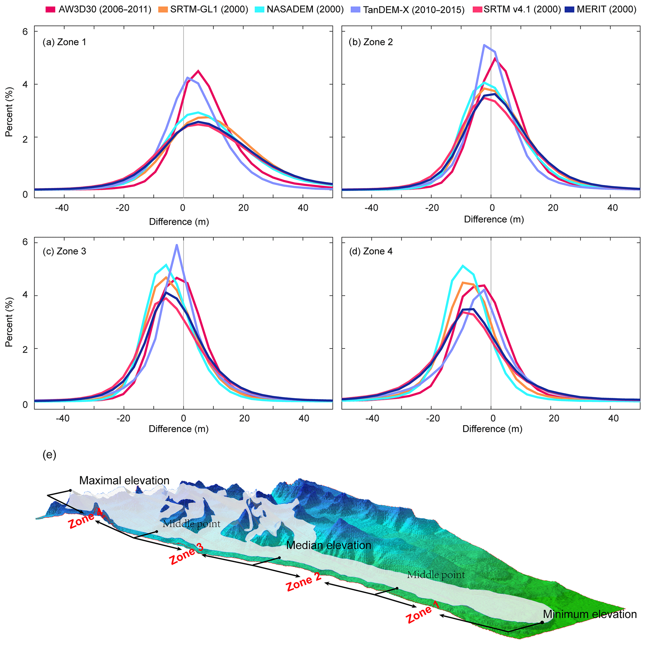
Figure 7 Probability distribution of the difference between six DEMs elevation and ICESat-2 elevation in different glacier zones (a–d) as defined in panel (e). The acquisition date of each DEM is labeled.

ME, MAE, and RMSE in Zone 3 and Zone 4, near or in the accumulation area, are almost all smaller than the corresponding values in Zone 1 (Fig. 7 and Table S1). The ME of all DEMs decreased to negative values in Zone 3 and Zone 4. Usually, in the accumulation area, glaciers have a positive or less negative elevation change (Li and Lin, 2017; Maurer et al., 2019; Rankl and Braun, 2016); therefore, accumulation may be concerned with changes in Zone 3 and Zone 4. The observed shift in the ME from Zone 1 to Zone 4 is a sign of influence from thinning or accumulation between the time of collection of the six DEMs and the ICESat-2 data.

In terms of SD, NASADEM performed best in Zone 3 and Zone 4, with values ranging from 8.8 to 11.1 m (Table S1). AW3D30 had the best performance of all DEMs in Zone 1 and Zone 2, with an SD varying from 10.0 to 12.3 m. The SD of TanDEM-X was better than that of SRTM v4.1 and MERIT in Zone 1 and Zone 2 but was worse in Zone 3 and Zone 4.

3.4 Sensitivity of modeled ice thickness to DEMs

The models are not adjusted independently according to the difference between the output and GPR results. Therefore, the results are not indicators of the performance of the models but rather references for examining the influence of different DEMs on ice thickness estimated using different ITIMs. The effects of the DEMs on the model outcomes are presented in Fig. 8 and are quite obvious. Mean ice thickness differs, according to the DEM used, by up to 134 %, 6 %, 47 %, and 19 % for GlabTop2, HF, ITIBOV, and OGGM, respectively. The deepest ice thickness differs by up to 53 %, 25 %, 13 %, and 13 % for GlabTop2, HF, ITIBOV, and OGGM, respectively.

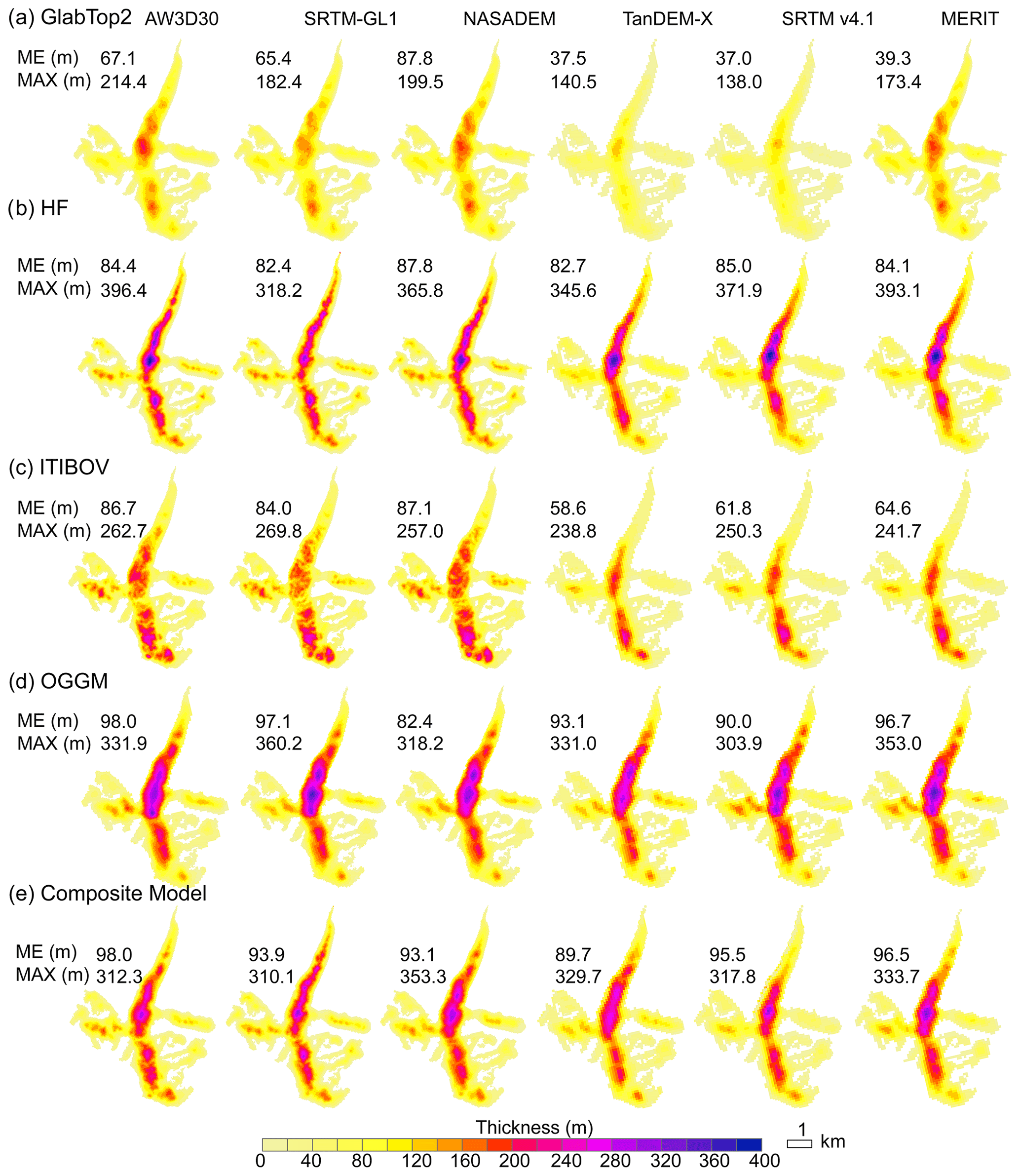
Figure 8 Distribution of modeled ice thickness of Chhota Shigri Glacier (location shown in Fig. 1) using AW3D30, SRTM-GL1, TanDEM-X, SRTM v4.1, NASADEM, and MERIT: (a) GlabTop2, (b) HF, (c) ITIBOV, (d) OGGM, and (e) composite result. Mean (ME) and maximum (MAX) modeled ice thickness are given in each panel.

The mean ice thicknesses from GlabTop2 and ITIBOV using the 90 m DEMs (they are TanDEM-X, SRTM v4.1, and MERIT) are ∼30 m less than those obtained when using 30 m DEMs (that is AW3D, SRTM-GL1, and NASADEM) (Fig. 8). GlabTop2, HF, and OGGM using AW3D30 and ITIBOV using NASADEM output the largest mean thickness. GlabTop2 and ITIBOV using TanDEM-X and OGGM and HF using SRTM-GL1 output the smallest mean thickness.

The influence of different DEMs on ITIMs can also be identified when making a comparison with the GPR results (Fig. 9 and Table 2). If the median error is used as the criterion, GlabTop2 and ITIBOV using NASADEM, HF using AW3D30, and OGGM using SRTM v4.1 achieved the relatively best simulation (Fig. 9). If RMSE was used, GlabTop2 using NASADEM, HF using SRTM-GL1, ITIBOV using AW3D30, and OGGM using TanDEM-X performed best (Table 2).

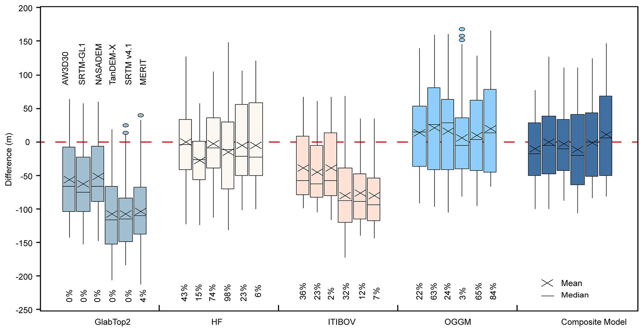
Figure 9 Point-by-point deviation comparison between the modeled and measured ice thickness from GlabTop2, HF, ITIBOV, OGGM, and the composite result. In each group, the boxes are plotted in the following order: AW3D30, SRTM-GL1, NASADEM, TanDEM-X, SRTM v4.1, and MERIT. Different models using the same DEM are aggregated by weights (labeled at the bottom) to achieve minimum mean absolute error.

Table 2 Root mean squared error (RMSE, m) of modeled ice thickness compared with ground-penetrating radar (GPR) measurements on each profile (Pf1 to Pf5). The locations of profiles are shown in Fig. 1. Bold numbers denote the best model performance on each profile using different DEMs.

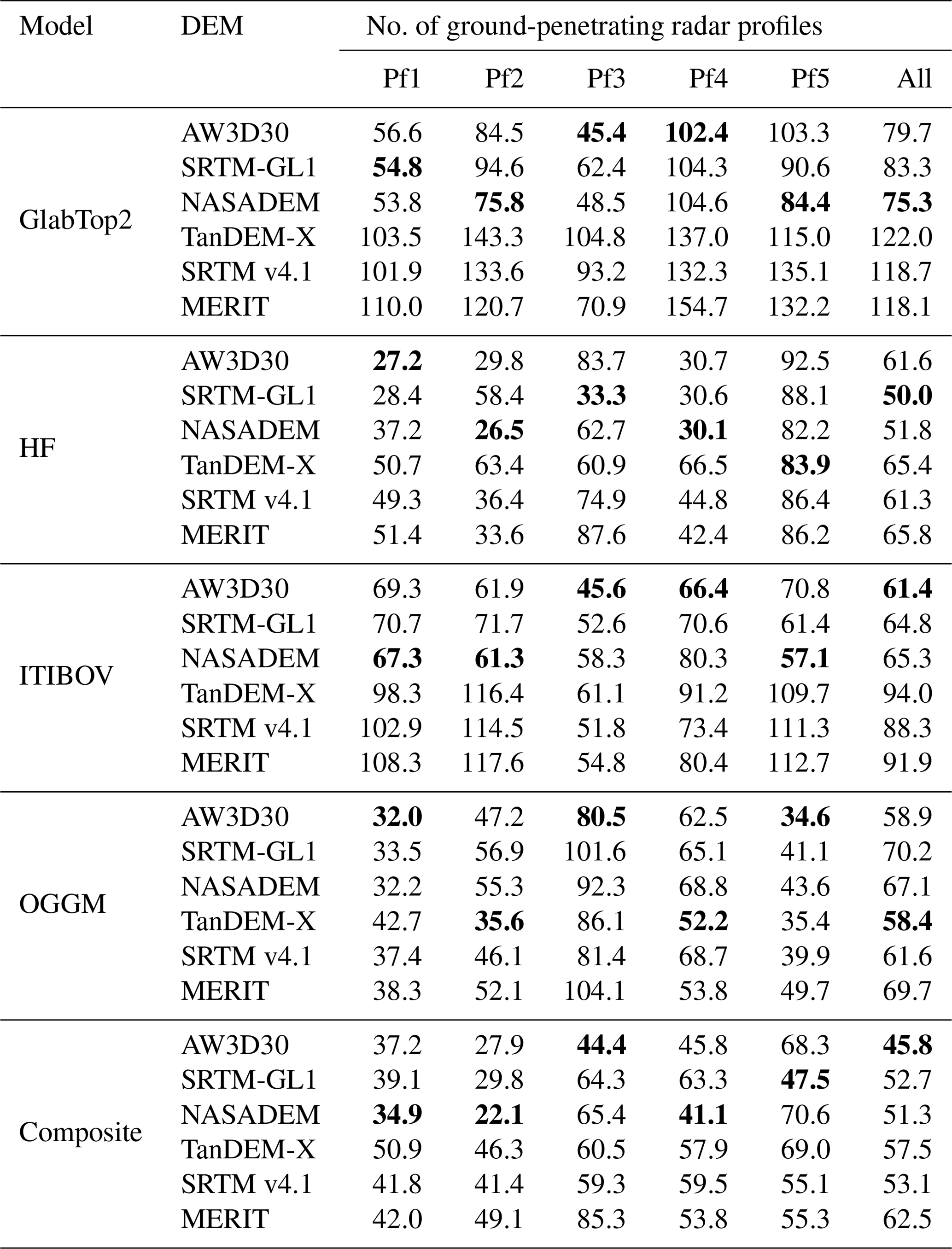
In different glacier zones, each DEM–model combination has its merits and weaknesses (Table 2). NASADEM indicates better performance (number of smaller RMSE values in five profiles) relative to other DEMs by using the GlabTop2 and ITIBOV models. AW3D30 conducts better by using the ITIBOV and OGGM models. TanDEM-X is better by using the OGGM model. While five models are composited, NASADEM behaves better. Overall, NASADEM and AW3D30 performs better in different glacier zones in all models.

Similar to the procedure of Farinotti et al. (2017), results from the four models are further composed to achieve the minimum MAE between the modeled and GPR thicknesses (Fig. 8e). The weights for each model in 10 experiments are shown in Table S2. After composition, the mean thickness using different DEMs ranged from 90 (acquired based on TanDEM-X) to 98 m (acquired based on AW3D30). NASADEM and AW3D30 achieved minimum MAE values, which are 36.7 and 44.1 m, respectively. RMSEs of combined ice thickness modeled from different DEMs are reduced by ∼21 m (∼25 %) when compared to the RMSE for one ITIM. The mean errors and median errors of all DEMs are at the range of ±10 m, except for that of AW3D30 and TanDEM-X, which is at a level of around 20 m. The spreads of error of 30 m DEMs are 33 % smaller than those of 90 m DEMs. The error spread from NASADEM was minimum (75.1 m), followed by AW3D30 (77.3 m).

4 Discussion

4.1 Influence of glacier elevation change on the assessment of DEMs

The identified extreme outliers (Fig. 3) are mostly located near the glacier terminus, high-elevation and high-slope regions (Fig. 10a and b). Extreme glacier melt, such as in southeastern Tibet, and surges, as observed in the Karakoram, can also lead to dramatic elevation changes, resulting in large differences (Fig. 10c). This glacier elevation change effect is also reflected in the spatial distribution of difference (Fig. 5), elevation bins (Fig. 6c), and glacier zones (Fig. 7). The differences at lower elevations are positive and generally decrease with elevation, consistent with the fact that glaciers melt at lower elevations and accumulate at higher elevations (Cuffey and Paterson, 2010). The differences in all DEMs with elevation and glacier zones comply with these features (Figs. 6c and 7). NASADEM was acquired in 2000, and TanDEM-X was acquired in 2010–2015, and the value of NASADEM is more positive than TanDEM-X in the ablation zone. The relatively more positive and larger values of ME and SD along the Hindu Kush–Himalaya, southern Tibet (Fig. 5), and negative ME values in the western Kunlun and Karakoram (Fig. 5) are also related to glacier elevation change (Hugonnet et al., 2021).

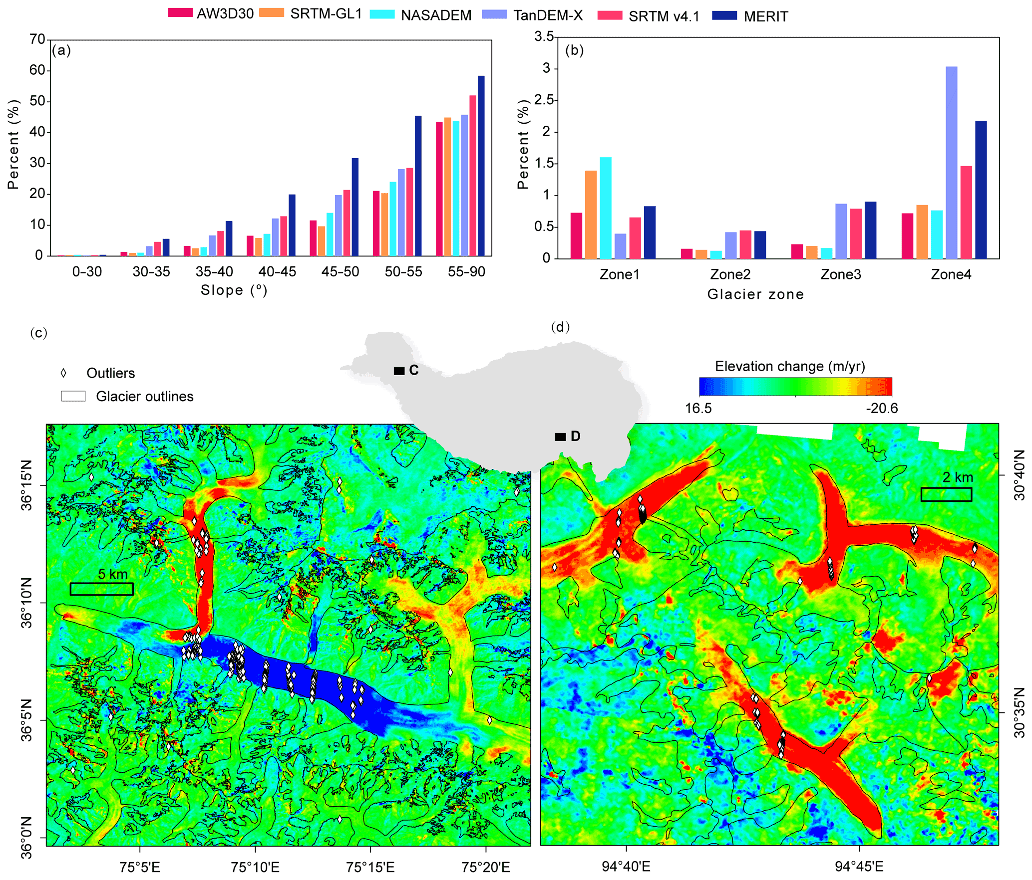
Figure 10 Distribution of excluded extreme outliers. The proportion of outliers accounting for the total number in slope bins (a) and each glacier zone (b). Examples of locations of excluded points overlaid with glacier surface elevation change in the Karakoram (c) and southern TP (d). Locations of these two examples in (c) and (d) are labeled C and D in the central insert, respectively. Glacier elevation change data covering 2000–2019 are from Shean et al. (2020).

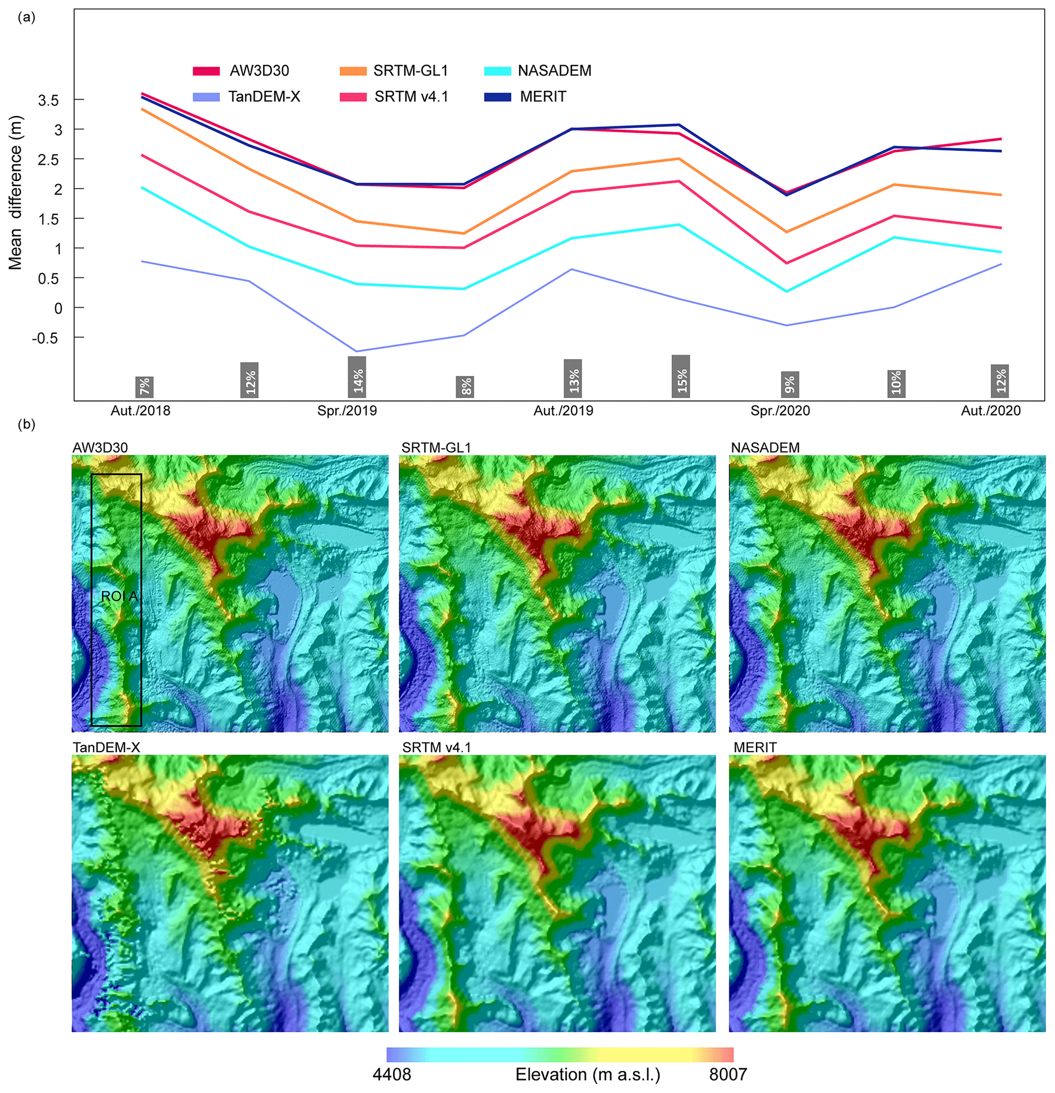
Figure 11 Influence on elevation differences between ICESat-2 and six DEMs from glacier elevation change and terrain factors. (a) Mean absolute difference between six DEMs and ICESat-2 in different seasons during 2018–2020. The spring, summer, autumn, and winter are defined as March–May, June–August, September–November, and December–February, respectively. The histogram at the bottom shows the percentage of the total number of points in each season. (b) Examples of elevation and shaded relief of six DEMs in the Shisha Pangma region. The rectangle denotes the area of interest.

After removing the glacier elevation change using the glacier elevation change dataset covering 2000–2018 (Shean et al., 2020), the mean difference in Zone 1 and Zone 2 decreased sharply by ∼14 and ∼7 m for the SRTM-based DEMs, respectively (Table 3). However, similar improvements are not obvious in Zone 3 and Zone 4. This may be related to the slight elevation change in the accumulation region (Brun et al., 2017; Shean et al., 2020) and high uncertainty due to steeper slopes and higher elevations (Fig. 6b and c). Apart from these factors, penetration depth of the C-band should be related to the remaining errors in the accumulation area. Mean errors in SRTM-based DEMs are 5.3–10.1 m in Zone 4, which are at the same order with the C-band penetration (Rignot et al., 2001). MAE, SD, and RMSE all improved a lot in four regions after this adjustment.

Table 3 Comparisons of differences between four SRTM-based DEMs and ICESat-2 elevation over glacier zones before and after adjustment. ICESat-2 data acquired in February are used to calculate the differences. Glacier zones are defined according to Fig. 7e.

ICESat-2 data covering the period from October 2018 to October 2020 repeat every 91 d. Therefore, variations of ICESat-2 elevation data caused by glacier fluctuations have influenced the error statistics (Fig. 11a). Precipitation on the TP mainly occurs in June–August (Maussion et al., 2014). Hence, after precipitation accumulation on glaciers in spring and summer, the elevation increased, and the mean difference decreased. With little accumulation, glaciers experience more melt and sublimation in autumn and winter (Li et al., 2018). As a result, the glacier surface elevation decreases, and the mean difference increases. However, the magnitude of these changes is much smaller, at a level of less than 3 m (Fig. 11a), compared with the large ME, MAE, and RMSE magnitude of most of the DEMs (with the exceptions of TanDEM-X and NASADEM) (Fig. 4). When taking all points from different seasons into consideration, the ICESat-2 dataset gives average elevation over the 2018–2020 period; the seasonal effects could also partly cancel each other out. If only the ICESat-2 data from February were used (Table 3), NASADEM and TanDEM-X still perform better than others. Therefore, we conclude that the seasonal fluctuations of ICESat-2 data have little influence on the assessments of the DEMs under the above conditions.

4.2 Influence of terrain on the assessment of DEMs

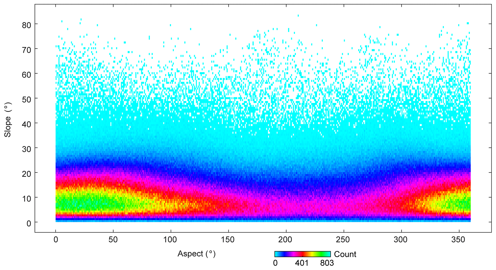
The elevation differences depend strongly on terrain factors (Fig. 6a and b). The largest errors are concentrated in the north aspect, as was also reported in previous studies (Gorokhovich and Voustianiouk, 2006; Shortridge and Messina, 2011), in which they were attributed to the orientation of the sensor (Gdulová et al., 2020; Shortridge and Messina, 2011). However, here, the data from different sensors all show this aspect dependence, and we infer that it may be related to the predominance of slopes for certain aspects. There are many more measurements with steeper slopes in the north aspect and fewer measurements with flatter slopes in the south aspect (Fig. 12). The error and spread become larger with steeper slopes (Fig. 7b), as also reported by Liu et al. (2019) and Uuemaa et al. (2020), which may be due to geometric deformation or shadow (Liu et al., 2019). Therefore, the error variation with aspect tends to be related to steeper slopes (Gdulová et al., 2020; Gorokhovich and Voustianiouk, 2006).

Figure 12 Distribution of measurements in different aspects against the slope.

Though points in the 55–90^∘ slope region account for a small fraction (Fig. 6d), almost half the points in the 55–90^∘ slope region are identified as extreme outliers (Fig. 10a). Differences also show large discrepancies for all DEMs in the steeply sloping regions where voids and large errors are frequent (Falorni, 2005). Steep slopes combined with low resolution led to variations in the spread of differences in Fig. 6b. Spreads of differences were larger on steep slopes for the 90 m DEMs than those of the 30 m DEMs. Intra-pixel variation aggravates this effect in steeply sloping regions (Uuemaa et al., 2020); lower-resolution or reduced-pixel DEMs smooth the terrain details and lead to inaccurate elevation compared with the 20 m footprint of ICESat-2 points. The spread and the number of outliers gradually increased with the slope, especially for the TanDEM-X case (Fig. 7b). Using the terrain in the rugged Shisha Pangma region (Fig. 12b) as an example, we can see that the elevation from TanDEM-X suffers from substantial errors along the ridge at high elevations, and the output appears almost blurred. Even so, TanDEM-X still has overall accuracy advantages over SRTM v4.1 and MERIT, indicating the high quality of TanDEM-X in low-relief regions (Fig. 7b).

4.3 Influence of misregistration on the assessment of DEMs

Six DEMs are produced from different sensors or by different methods. Pixels in DEMs do not represent exactly the same location. This misregistration among DEMs, which has been ignored in previous research (González-Moradas and Viveen, 2020; Liu et al., 2019), is an important error source when looking at DEM differences (Hugonnet et al., 2021; Van Niel et al., 2008). This study intends to give direct insights into the quality of uncorrected DEM products, so the misregistration problem was not tackled before the evaluations were carried out. However, the influence of misregistration was evaluated. According to the sinusoidal relationship between aspect and error differences between two DEMs (Van Niel et al., 2008), using the co-registration method in Nuth and Kääb (2011) and ICESat-2 points outside the glaciers, offset pixels relative to ICESat-2 in the x and y direction at the $\mathrm{1}{}^{\circ }\times \mathrm{1}{}^{\circ }$ grid scale were estimated by a nonlinear least-squares fitting method across the TP. Misregistration was found to be less than one grid spacing (Fig. 13). The misregistration of SRTM-GL1 relative to ICESat-2 is the largest; the misregistration of other DEMs is always less than 0.2 grid spacings. Considering that only the cell center value was used, the sub-grid spacing shift may have little influence (Van Niel et al., 2008).

Figure 13 Distribution of offset grid spacings of DEMs relative to ICESat-2 on a $\mathrm{1}{}^{\circ }\times \mathrm{1}{}^{\circ }$ grid. Only the grid squares with R² greater than 0.5 and the number of records greater than 1000 are considered.

4.4 Influence of DEMs on ice thickness estimated by ITIMs

Even with the same parameters, the same ITIM using different DEMs will yield different thickness patterns (Figs. 8 and 9). The quality of a DEM indeed influences the performance of the ITIMs. However, the different models have various levels of robustness to the quality of the input DEMs. Different DEMs resulted in differences in the largest and smallest mean ITIM ice thickness at a range of 3.6–32 m (Fig. 8).

Generally, the outcome with GlabTop2 and ITIBOV using 30 m DEMs is 51 % and 43 % better than with the 90 m DEMs in mean error, respectively. With GlabTop2, elevation data were used to determine not only the slope but also the shear stress (Frey et al., 2014). A sensitivity test based on Eqs. (1)–(4) was executed, and the modeled ice-thickness differences before and after adding perturbations to the input parameters such as slope and elevation were compared. An error of +5^∘ in slope caused more than a −34.1 % difference in the output for slopes of less than 20^∘. Additionally, relative elevation errors had an enormous impact (Fig. 14b). For glaciers with an elevation range of less than 400 m, which accounted for 41 % of the total number and 5 % of the total area over the TP, +10, +30, and +50 m errors in elevation range caused more than +2 %, +6 %, and +10 % differences in output. Such errors in elevation range had greater influence (Fig. 14b), especially for small glaciers, which have smaller elevation ranges. These two errors propagate and lead to a much larger overall error (Table 3). Thus, GlabTop2 using NASADEM and AW3D30 with the best quantity as input achieved the best RMSE in comparison with GPR measurements. In contrast to the other ITIMs, the ITIBOV model directly estimated the ice thickness at each grid cell according to cell velocity information without interpolation. The slope sensitivity of ITIBOV is higher than that of GlabTop2, with an error of +5^∘ in slope causing more than a −71.4 % difference in the ice thickness for slopes of less than 20^∘ (Fig. 14a). The flatter the slope is, the more sensitive ITIBOV is to the slope error (Fig. 14a). Although along- and across-track slope data are provided in the ICESat-2 ATL06 product, they are incompatible with the slope estimated from DEMs due to their different data formats and algorithms used (Burrough and McDonell, 1998; Smith et al., 2019). Moreover, the surface terrain of glaciers changes with time due to accumulation, melting, and transient dynamics (Dehecq et al., 2019; Shean et al., 2020). Nevertheless, the accuracy of the DEMs estimated here could also provide some information about slope accuracy. With the higher-accuracy NASADEM and AW3D30 as input of ITIBOV, most accurate ice thicknesses were obtained (Table 2).

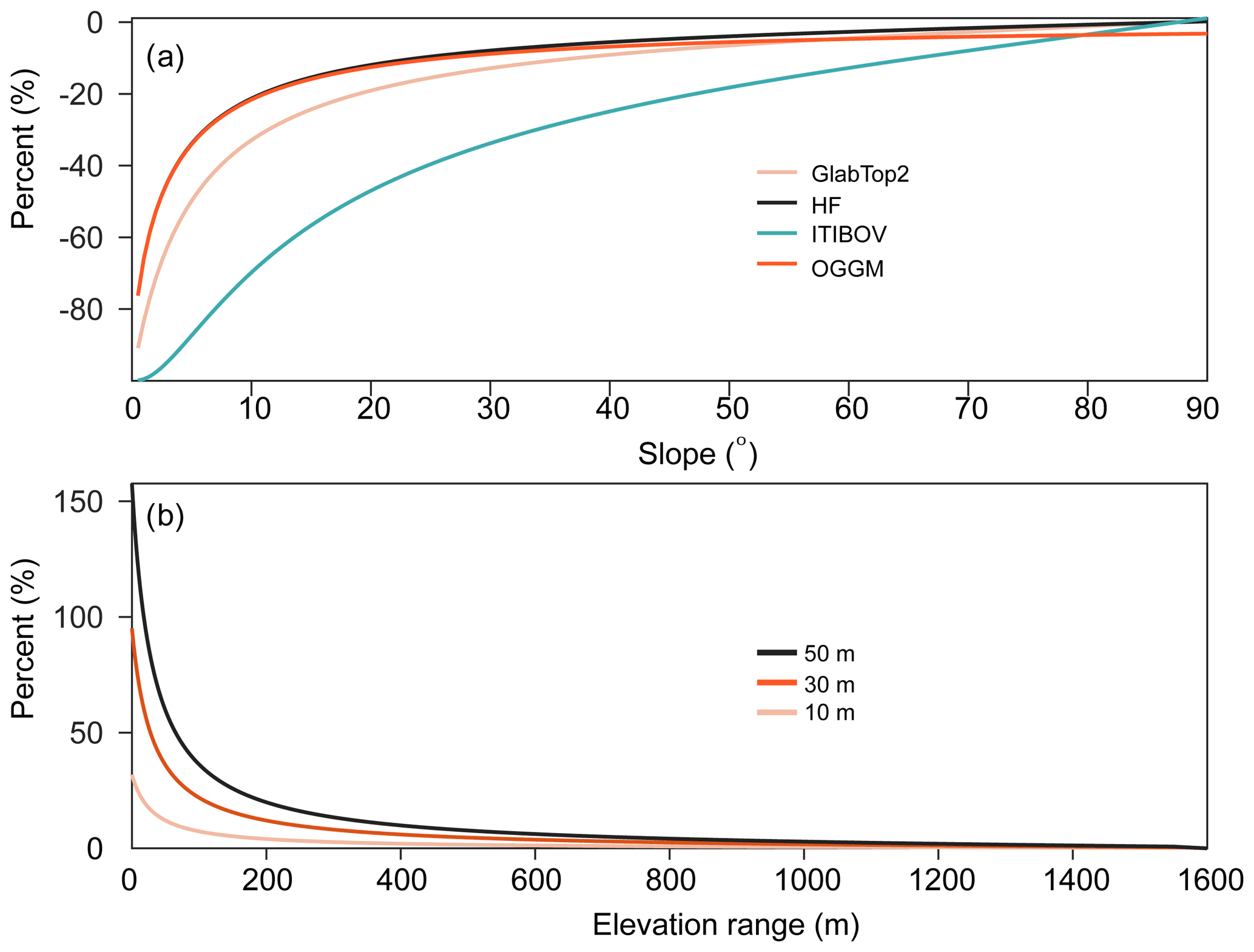
Figure 14 Sensitivity test of slope and elevation on ice-thickness inversion models. (a) Percentage difference of modeled ice thickness from GlabTop2, HF, ITIBOV, and OGGM when there is +5^∘ slope error. (b) Percentage difference of modeled ice thickness from GlabTop2 when the elevation range error is +10, +30, and +50 m for different elevation ranges.

For HF and OGGM, the modeled ice thicknesses did not show large differences when using 30 or 90 m DEMs as input (Fig. 9), thereby suggesting a minor impact of DEM resolution on ice-thickness reconstruction (Pelto et al., 2020). In the HF model, elevation data were used for convergence calculation of apparent mass balance and mean slope in elevation bins (Farinotti et al., 2009, 2019), whereas, in OGGM, it is used to extract flowlines, shear stress at flowlines, and mass balance at an elevation (Maussion et al., 2019). These two models show roughness to the input DEM (Fig. 14a). Although NASADEM and TanDEM-X were more accurate, the output of HF and OGGM using these two DEMs did not yield better results compared to when using the other DEMs (Fig. 9). The SD of RMSE values for HF and OGGM using six DEMs are 6.2 and 4.9 m, respectively (Table 2). The SD of mean ice thickness by HF and OGGM using six DEMs are 1.1 and 6.0 m (Fig. 8).

When the results from different ITIMs are ensembled, the influences of uncertainty and resolution in the input DEMs on the modeled ice thickness still exist (Fig. 9 and Table 2). The RMSE of ITIMs from 30 m DEMs was 16.8 % less than that from 90 m DEMs. Models using AW3D30 and NASADEM, which have higher resolution and better accuracy, yielded the most accurate thickness estimates. However, glacier surface elevation changes with climate; AW3D30 acquired in different years and seasons represents glacier terrain in different periods. This could result in the spatial inconsistencies of the output of ITIMs in large-scale ice-thickness inversion. Above, we suggest NASADEM as the best input of ITIMs for ice-thickness estimates over the TP. This conclusion is of significance for ice-thickness inversion models using DEMs in the TP. However, it should be noted that the result may be not suitable for studies in other glacierized mountainous regions. Because various errors exist in DEMs, such as speckle noise, stripe noise, and absolute bias, they behave differently across the earth (Yamazaki et al., 2017; Takaku et al., 2020). Our method to assess the accuracy of DEMs is repeatable in different regions, combined with the recently released glacier elevation change data on earth (Hugonnet et al., 2021). Furthermore, benefiting from the high accuracy and dense coverage of ICESat-2 data, the quality of DEMs can also be improved, similar to what has been done in the production of MERIT (Yamazaki et al., 2017). For example, the misregistration in DEMs could be corrected, and terrain-related errors could be reduced by unitizing the relation of difference against slope, aspect, and elevation in Fig. 6.

5 Conclusions

In the present study, six DEMs (i.e., AW3D30, SRTM-GL1, NASADEM, TanDEM-X, SRTM-GL1, and MERIT) from different sensors with different spatial resolutions were evaluated using ICESat-2 data. The influence of glacier dynamics, terrain, and misregistration on the DEM accuracy was analyzed. Out of the three 30 m DEMs, NASADEM was the best performer in vertical accuracy with an ME of 0.9 m and an RMSE of 12.6 m. Out of the three 90 m DEMs, TanDEM-X performed best with an ME of 0.1 and an RMSE of 15.1 m. The quality of TanDEM-X was stable and unprecedented on shallow slopes but suffered from serious problems on steep slopes, especially along the steep ridges. AW3D30 has similar accuracy to NASADEM and is even better in SD, MAE, and RMSE when not considering the effect of glacier dynamics. SRTM-based DEMs (i.e., SRTM-GL1, SRTM v4.1, and MERIT) (∼15 m RMSE) were inferior to NASADEM. MERIT shows little improvement over SRTM v4.1 in glacierized terrain. The influence of glacier elevation change on the elevation difference is larger for DEMs acquired in an earlier period, at low elevations, and in the ablation region. However, this does not influence the conclusion that NASADEM performed the best, followed by TanDEM-X but with serious outliers in the high-elevation region. For all the DEMs, the errors increased from the south-aspect slope to the north-aspect slope, controlled by the increasing error with slope. Misregistration errors in the glacier region are within one grid spacing and have little influence on the evaluation benefiting from the 20 m footprint of ICESat-2 relative to the 30 or 90 m resolution DEMs.

The influence of DEM accuracy on ice-thickness inversion models depends on the model properties. Generally, a higher-resolution DEM was helpful for better model outcomes. The widely used GlabTop2 model is very sensitive to the accuracy of both elevation and slope; using NASADEM as input, this model facilitated the best outcome. Although the OGGM and HF models are less sensitive to the quality of DEM, the use of NASADEM or AW3D30 was still beneficial. Among the four ice-thickness inversion models, ITIBOV was the most sensitive to slope accuracy. Ice-thickness inversion models using AW3D30 or NASADEM as input gave the most accurate thickness estimates. These two DEMs also perform the best when four ice-thickness inversion results were aggregated by the minimum MAE optimization method.

Considering the influence of inconsistency in data acquisition time on generating glacier terrain, we suggest that NASADEM is the best choice for ice-thickness inversion models over the whole TP. AW3D30 could be a good substitute but with limitations from its mixed acquiring dates. TanDEM-X is an appropriate alternative for glaciological research focusing on the flat glacier terminus, but it requires further improvement for use in steep terrain or ice-thickness inversion.