the Creative Commons Attribution 4.0 License.
the Creative Commons Attribution 4.0 License.
 | 06 May 2022
Polarimetric radar reveals the spatial distribution of ice fabric at domes and divides in East Antarctica
M. Reza Ershadi
Reinhard Drews
Carlos Martín
Olaf Eisen
Catherine Ritz
Hugh Corr
Julia Christmann
Ole Zeising
Angelika Humbert
Robert Mulvaney
Ice crystals are mechanically and dielectrically anisotropic. They progressively align under cumulative deformation, forming an ice-crystal-orientation fabric that, in turn, impacts ice deformation. However, almost all the observations of ice fabric are from ice core analysis, and its influence on the ice flow is unclear. Here, we present a non-linear inverse approach to process co- and cross-polarized phase-sensitive radar data. We estimate the continuous depth profile of georeferenced ice fabric orientation along with the reflection ratio and horizontal anisotropy of the ice column. Our method approximates the complete second-order orientation tensor and all the ice fabric eigenvalues. As a result, we infer the vertical ice fabric anisotropy, which is an essential factor to better understand ice deformation using anisotropic ice flow models. The approach is validated at two Antarctic ice core sites (EPICA (European Project for Ice Coring in Antarctica) Dome C and EPICA Dronning Maud Land) in contrasting flow regimes. Spatial variability in ice fabric characteristics in the dome-to-flank transition near Dome C is quantified with 20 more sites located along with a 36 km long cross-section. Local horizontal anisotropy increases under the dome summit and decreases away from the dome summit. We suggest that this is a consequence of the non-linear rheology of ice, also known as the Raymond effect. On larger spatial scales, horizontal anisotropy increases with increasing distance from the dome. At most of the sites, the main driver of ice fabric evolution is vertical compression, yet our data show that the horizontal distribution of the ice fabric is consistent with the present horizontal flow. This method uses polarimetric-radar data, which are suitable for profiling radar applications and are able to constrain ice fabric distribution on a spatial scale comparable to ice flow observations and models.
- Article
(7582 KB) - Full-text XML
- BibTeX
- EndNote


The movement of glaciers and ice sheets has two components: ice deformation and basal sliding. Satellites provide widespread and increasingly well-resolved temporal surface velocities. In most cases, however, it is difficult to differentiate the contribution of ice deformation and basal sliding. This results in increased uncertainty in several areas, such as ice flow model initialization with data assimilation techniques (Schannwell et al., 2019) or predicting erosion rates from surface velocities (Headley et al., 2012; Cook et al., 2020). Even in ice-sheet-covered areas where basal sliding can certainly be excluded, e.g., near ice domes or beneath ice rises (Matsuoka et al., 2015), knowledge of internal ice deformation is important for predicting age–depth relationships for new ice core drill sites (Parrenin et al., 2007; Martín et al., 2009; Martín and Gudmundsson, 2012) or for using internal layer architecture to reconstruct paleo-ice dynamics (Matsuoka et al., 2015). The temperature-dependent, non-linear, and anisotropic rheology of ice governs how ice deforms and poses many challenges to numerical ice flow models. Most models do not consider ice fabric anisotropy because this quantity is currently poorly constrained by observations. The most reliable observations of ice fabric come from the analysis of thin ice core sections using ice fabric analyzers detecting single ice crystals' lattice orientation using transmitted light microscopy (Durand et al., 2009; Weikusat et al., 2017). The underlying principle used is that single ice crystals are uniaxially birefringent for electromagnetic waves. This causes the polarization-dependent formation of ordinary and extraordinary waves that propagate through the lattice and superimpose with a phase shift at the detector. Constructive and destructive superposition of these waves can be used to characterize ice fabric in thin sections at a vertical spacing of centimeters to decimeters (Kerch et al., 2020). Ice-penetrating radar on ice sheets employs a similar principle to optical methods but slightly different because it is based on measuring a bulk anisotropy rather than an intrinsic. In comparison, the dielectric anisotropy of ice observed by radar is a combined effect of the ice crystal birefringence and crystal-orientation fabric with different spatial scales and applied electromagnetic frequencies. As is explained in more detail below (Sect. 3.3), ground-penetrating radar systems such as the ground-based autonomous phase-sensitive radio echo sounder (ApRES) (Brennan et al., 2014; Nicholls et al., 2015) can detect the polarization-dependent phase shift induced by ice birefringence and also quantify the degree of anisotropic scattering which may be caused by abrupt vertical changes in ice fabric. Other geophysical methods to detect ice fabric anisotropy are sonic logging of boreholes (Gusmeroli et al., 2012; Pettit et al., 2007) or surface-based seismic surveys (Diez and Eisen, 2015; Diez et al., 2015; Smith et al., 2017; Brisbourne et al., 2019).
Ice-core- and borehole-based methods are reliable and can be obtained in a high vertical resolution (sub-centimeter scale). However, in deep ice, where grains may be large compared with the typical ice core diameter of 10 cm, they are statistically not well constrained. They also do not provide much spatial context and are often obtained at dome locations where the horizontal advection is negligible, and the climate record is easier to interpret. The surface seismic methods are more challenging in terms of field logistics, but they inherently provide wide-angle information, which radar typically does not. The majority of radar profiles are not analyzed with respect to ice fabric anisotropy often because the radar systems do not provide the required precision or are collected with a single polarization only. The collection of crossing radar lines partially remedies this issue. However, newer radar systems collect data with cross-polarized arrays so that area-wide detection of ice anisotropy appears to be a target within reach (Yan et al., 2020). The theory of radar birefringence in glaciology has long been known (Hargreaves, 1978; Woodruff and Doake, 1979; Matsuoka et al., 1997; Fujita et al., 1999) and has recently been significantly extended to exploit the capacity of phase information from newer radar systems that were previously not available (Dall, 2010; Jordan et al., 2019, 2020). Examples for applications of radar polarimetry exist near ice domes in Greenland (Gillet-Chaulet et al., 2011; Li et al., 2018; Jordan et al., 2019) and Antarctica (Fujita et al., 1999; Brisbourne et al., 2019), on ice rises (Drews et al., 2015; Matsuoka et al., 2015; Brisbourne et al., 2019), in flank-flow regimes (Eisen et al., 2007), in divides (Young et al., 2021), and for ice streams (Jordan et al., 2020). However, there is not yet a clear observation-based picture of how ice fabric develops across the different flow regimes.
Here, we built on a previously derived forward modeling framework (Fujita et al., 2006) that can model polarimetric backscattered signal as a function of vertical distribution of ice fabric, extended by Jordan et al. (2019, 2020). We develop it further with theory relating to anisotropic reflections and then develop an inverse approach that also attempts to characterize ice fabric types continuously along depth and for all of the three bulk crystallographic axes. The technical developments will allow the ice fabric orientation to be automatically georeferenced and its full variability with depth to be reconstructed. But the major achievement in this method is to estimate the depth variability in the horizontal ice fabric anisotropy along with reflection ratio, which allows all the possible eigenvalues of the ice fabric to be estimated. This leads to quantifying the ice fabric type and its vertical anisotropy. We demonstrate this for 21 ApRES measurements conducted near two ice core drill sites drilled by the European Project for Ice Coring in Antarctica (EPICA). Of the radar measurements, 20 cover the dome–flank transition at the EPICA ice core site in Dome C (EDC) and one additional measurement at the EPICA ice core site in the eastern Dronning Maud Land (EDML). The successful validation with ice core data suggests that polarimetric radar is now capable of providing all directional constraints required for parameterization of an anisotropic flow law.
We use radar data near two deep ice core drill sites in East Antarctica. One is located at Dronning Maud Land (DML), near the German summer station (Kohnen at −75.00∘ S, 0.00∘). The other site is located at Dome C, close to Concordia station (−75.10∘ S, 123.35∘ E). We use the measured ice fabric data from both ice cores published by Weikusat et al. (2017) and Durand et al. (2009), respectively, to validate our polarimetric-radar data inferences. At Dome C, radar data were additionally collected at 20 stations along with a 36 km long profile across the dome, enabling us to track ice fabric variability in the dome–flank transition zone. Surface topography at Dome C (Helm et al., 2014; Howat et al., 2019) exhibits an ice dome elongated in the SW–NE direction (Fig. 1a). Surface velocities are too slow (<0.02 m a−1) for reliable detection with satellite imagery. GPS measurements show that the ice flow direction follows the surface maximum gradient direction, increases with distance from the dome, and is near-parallel to the transect described above (Vittuari et al., 2004). The Kohnen station (Fig. 1b) is located near a transient ice-divide triple junction in a flank-flow regime, and the ice flow is significantly faster (≈0.74 m a−1) than at Dome C. The largest principal strain rate at Dome C and EDML is oriented SW–NE (Rémy and Tabacco, 2000; Vittuari et al., 2004) and 24∘ N (Wesche et al., 2007; Drews et al., 2012), respectively.
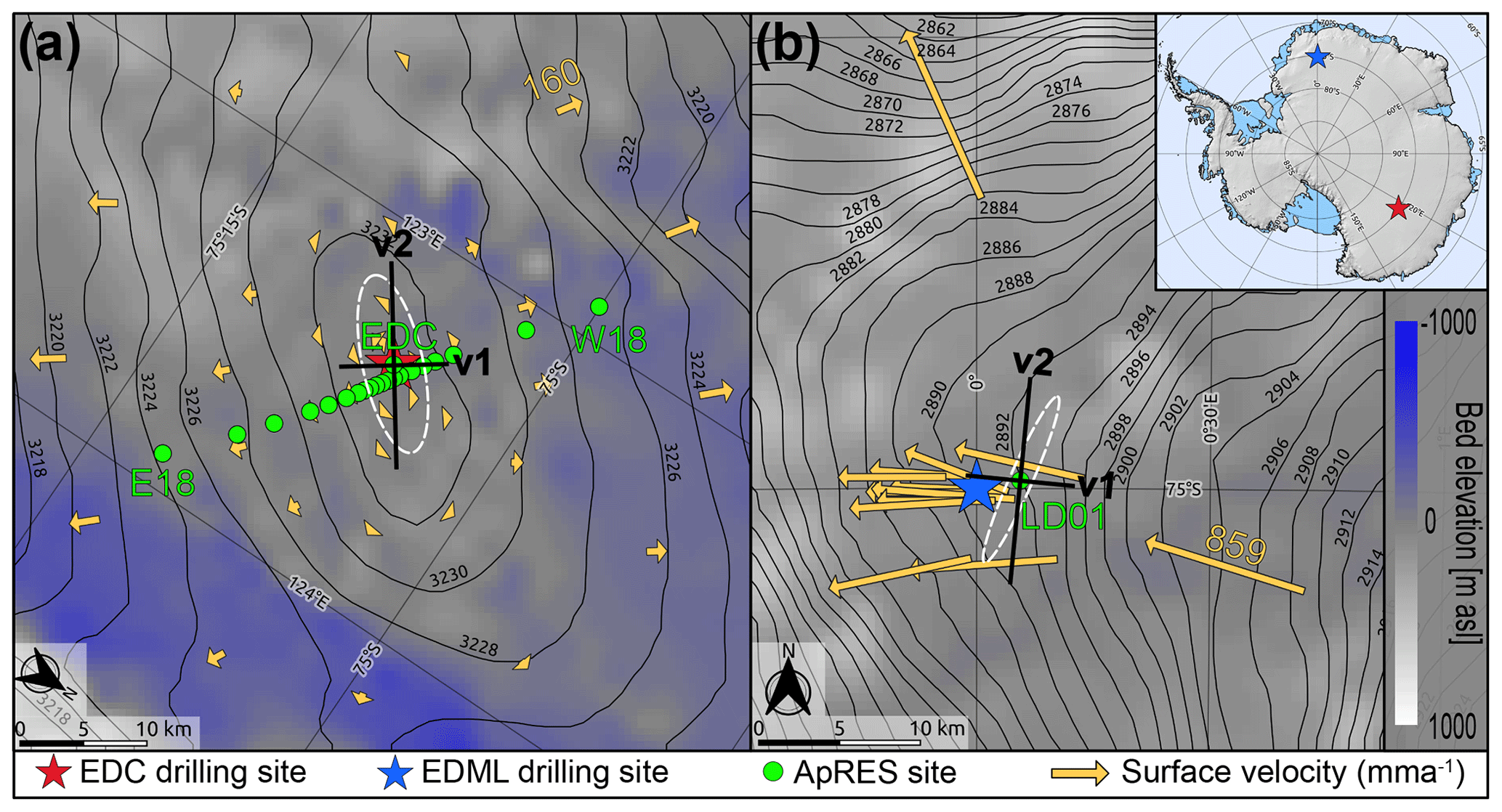
Figure 1Map of the study areas. (a) EPICA Dome C (EDC). (b) EPICA Dronning Maud Land (EDML). Black contour lines are the surface elevation (Helm et al., 2014). The background color is the bed elevation (Morlighem et al., 2020). Yellow arrows are the magnitude and direction of the surface velocities at EDC (Vittuari et al., 2004) and EDML (Wesche et al., 2007). The white strain ellipses mark the directions of the maximum and minimum strain rate. The ice fabric's horizontal eigenvectors are represented by v1 and v2, and they are based on the results in Sect. 4.1 and 4.2. Note that (a) and (b) have a different scale and orientation.
3.1 Quantitative metrics used to define the ice fabric
Ice crystallizes in the shape of hexagons, and the direction normal to the basal plane is described with the c axis (Hooke, 2005). Ice crystals are strongly anisotropic and 60 times softer along the basal plane than perpendicular to it (Duval et al., 1983; Smith et al., 2017). In a given strain regime, individual ice crystals deform preferentially along the basal plane and orient themselves so that the bulk c-axis orientation forms a distinct pattern, which we refer to as ice fabric. Elsewhere it is also described as crystal-orientation fabric (COF) or lattice-preferred orientation (LPO) (Weikusat et al., 2017). The radio waves are sensitive to the dielectric anisotropy, which follows the mechanical anisotropy described by the second-order orientation tensor (Gödert, 2003; Gillet-Chaulet et al., 2006; Martín et al., 2009). The bulk ice fabric pattern is described with a second-order orientation tensor (we refer to this as orientation tensor) using the eigenvectors and v3 and eigenvalues and λ3 of an ellipsoid that best represents the average c-axis orientation of all ice crystals in the sample. The eigenvalues are normalized
and to be consistent with the past polarimetric-radar studies, we assume
Combination of Eqs. (1) and (2) set bounds on the eigenvalues (, , and ). The eigenvalues can be used to distinguish the ice fabric types such as isotropic (), girdle (), and single maximum () (Woodcock, 1977; Azuma, 1994; Fujita et al., 2006). The eigenvalues and eigenvectors can be used to describe the dielectric permittivity tensor ε′, containing the bulk permittivities and relevant for radio wave propagation (Sect. 3.3).
3.2 Data collection
The radar data in this study were collected using a phase-sensitive frequency-modulated continuous-wave radar system (Brennan et al., 2014; Nicholls et al., 2015) with a 200 MHz bandwidth and fc=300 MHz center frequency. This radar emits linearly polarized electromagnetic waves using a slot antenna where the direction of the polarization plane is aligned with the direction of the electric field vector (E) in the antenna as shown in Fig. 2a.
We use terminology from satellite radar polarimetry to distinguish the directions of the polarization with H and V, although, in a nadir-looking geometry, these are arbitrarily determined because H and V both have horizontal polarization plane at depth. Here, we name the horizontal (H) and vertical (V) polarization plane consistent with Jordan et al. (2019). However, we want to point out that this definition is different to the one applicable to seismic shear waves, where vertical receivers have a vertical component upon reflection at depth for non-vertical angles of incidence, and vice versa.
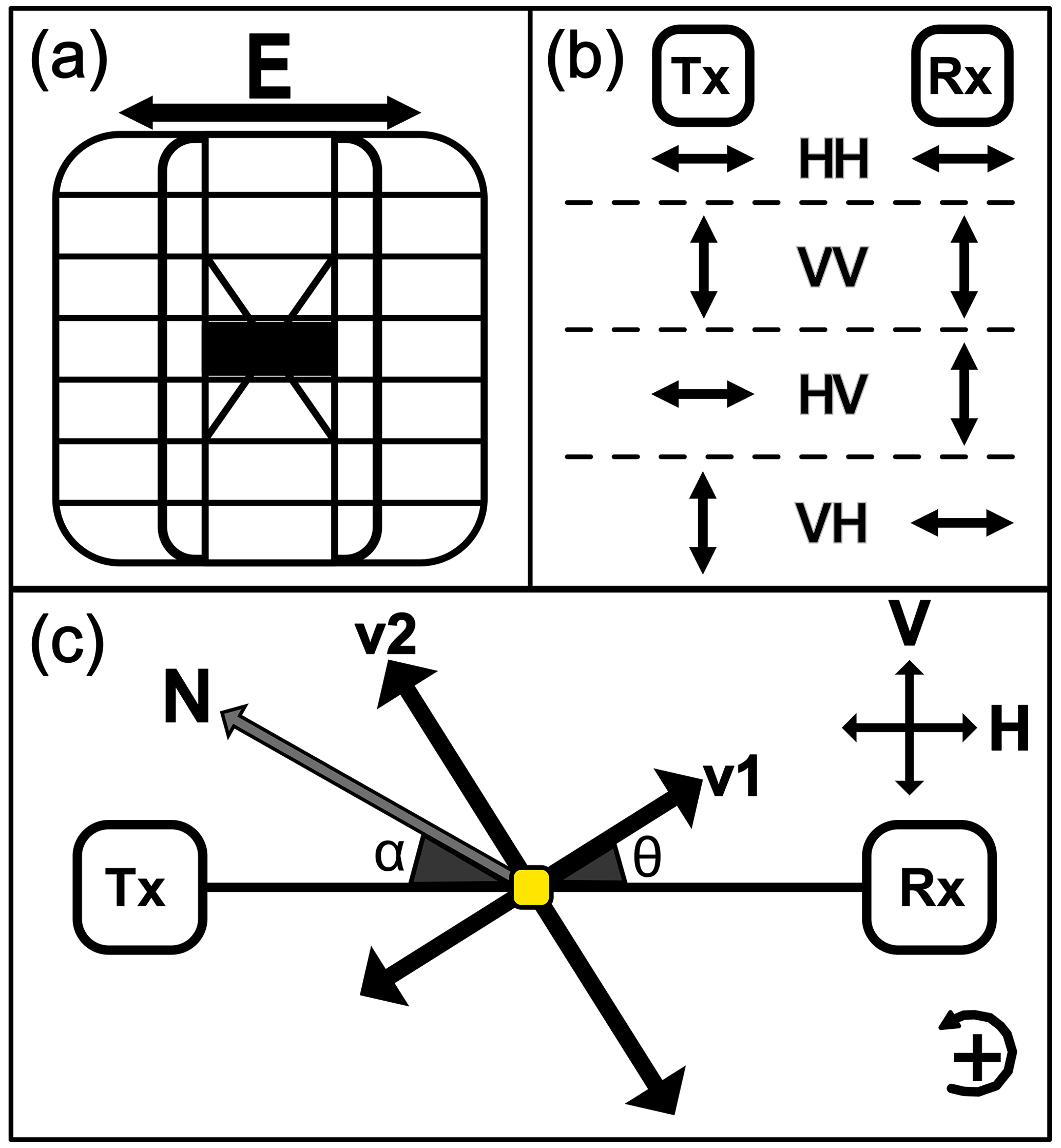
Figure 2(a) Bird's-eye view of the ApRES slot antenna with the direction of the electric field vector (E). (b) The terminology of the co- and cross-polarized ApRES measurements defined using E. The direction of wave propagation is into the page (⊗). (c) The model coordinate system where transmitting (Tx) and receiving (Rx) antennas are connected with the aerial line (TR). The horizontal (H) and vertical (V) polarization planes are defined so that H is parallel to TR. The directions of the ice fabric horizontal principal axes are represented by v1 and v2. θ is the angle between H and v1, and α is used for georeferencing.
The model coordinate system is shown in Fig. 2c. The aerial line (TR) connects transmitter (Tx) and receiver (Rx), and by convention, we assume that H is parallel to TR; v1 and v2 are the horizontal eigenvectors which align with the direction of the smallest () and largest () horizontal principal permittivity, respectively (Fujita et al., 2006; Jordan et al., 2019). Hence, if H is aligned with v1. The angle α is measured by compass with uncertainty for georeferencing the data. Here, we use polar stereographic coordinates, where counterclockwise rotation is positive.
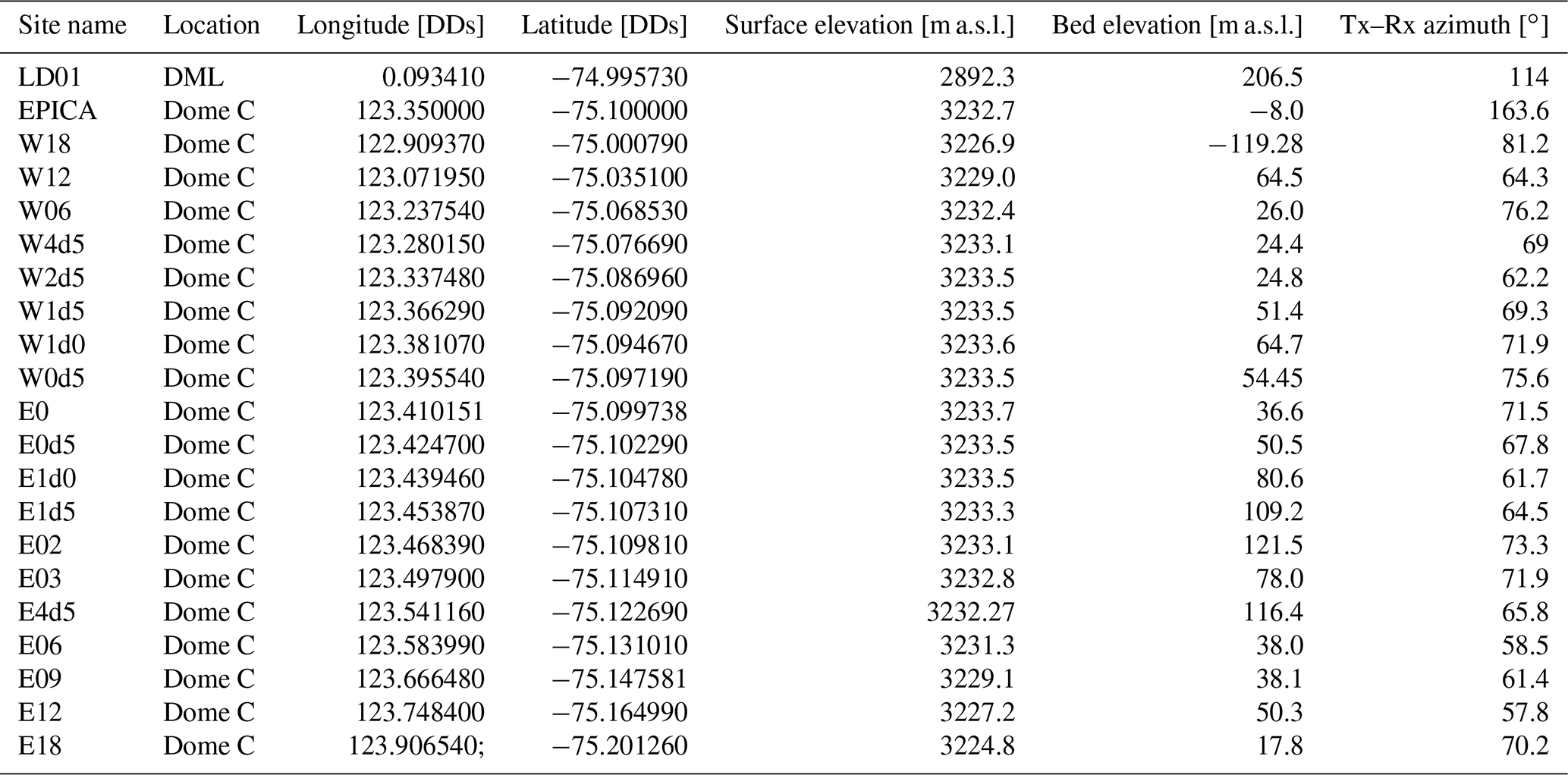
Radar data at all the sites were collected at a fixed α, obtained from different antenna orientation in co-polarization (HH, VV) and cross-polarization (HV, VH) configurations (Hargreaves, 1977; Fujita et al., 2006) as shown in Fig. 2b. We refer to these measurements as quad-polarimetric measurement. Radar data at Dome C were collected at 20 sites in January 2014. One of the sites is located within walking distance of the ice core site EDC. The remaining 19 sites (termed E(ast)0-E18, and W(est)0.5-W18, with the numbers relating to the distance in kilometers away from the dome) are aligned in a profile which is approximately perpendicular to the long axis of the dome and parallel to the flowline (Fig. 1a). At EDML, data were collected in January 2017, approximately 2.7 km northeast of the ice core site EDML (Fig. 1b). More information related to the individual ApRES sites is shown in Appendix A.
3.3 Background of radar polarimetry
Radio signal propagation through ice sheets is polarization-dependent because of the dielectric anisotropy of the ice fabric. If the direction of v3 is vertical, and the remaining two eigenvectors (v1,v2) are in the horizontal plane, then the relation between the depth profile of the dielectric permittivity tensor and the orientation tensor is given by Fujita et al. (2006):
For the dielectric permittivity at radio frequencies perpendicular to c axes, we use (Fujita et al., 2000), which is slightly lower than the value found by Bohleber et al. (2012). The value of a dielectric anisotropy for a single crystal is set to (Matsuoka et al., 1997). The vertical v3 assumption in this study is justified through measurements at the EDC ice core, where the direction of v3 varies only by about 5∘ around the vertical (Durand et al., 2009). Elsewhere in ice sheets, this may not be the case, which will cause an additional source of horizontal birefringence (Matsuoka et al., 2009; Jordan et al., 2019).
We model radio wave propagation through birefringent ice using the method developed by Fujita et al. (2006). It includes transmission and reflection of initially linearly polarized waves emitted with two polarization modes (H and V, with direction defined in the previous section). If z is the depth from the surface (positive downward), it assumes stratified ice with layers predicting the radar response as a function of the emitted polarization plane and ice fabric parameters. Radar transmission (T) and reflection (Γ) are represented by 2×2 matrices only because radar signal propagation is insensitive to the vertically directed v3. The transmitted radar wave ET and the corresponding radar reflection ER are 2×1 vectors, with each component containing the electric field information of the H and V polarization components, respectively (Doake et al., 2002). Because only relative phase and amplitude variations are considered, all information about the radio wave transmission and reflection can be inferred from the scattering matrix (S) at layer N:
containing the complex scattering unit
where D and R are the depth factor and rotation matrix, respectively. The four elements of the scattering matrix are described as co-polarized scattering signals (sHH and sVV) and cross-polarized scattering signals (sHV and sVH).
To consider the polarization dependence of the reflection boundary, we formed the reflection ratio
where Γx and Γy are the elements of the reflection matrix Γ known as complex amplitude reflection coefficients (Ackley and Keliher, 1979; Ulaby and Elachi, 1990; Fujita et al., 2000, 2006). Here we only use the real part of Γx and Γy. Therefore, r is a scalar quantity. Further details about the radar forward model implementation and definition of all the parameters in Eq. (5) are described in Appendix B and Fujita et al. (2006).
The parameters of interest that we aim to infer from the radar observations for each layer are the horizontal anisotropy , the ice fabric orientation angle θ, and the reflection ratio r. All of these quantities may vary with depth. Much information is gained by interpreting the coherence phase difference between sHH and sVV, which is a crucial development in the works from Dall (2010), extended by Jordan et al. (2019). The coherence phase difference ϕHHVV is the argument of the complex polarimetric coherence CHHVV, estimated via a discrete approximation,
with * as a complex conjugate,
where M is the number of range bins used for vertical averaging, and b is the summation index. The depth gradient of ϕHHVV provides a way to relate the local phase gradient to Δλ at the direction of the horizontal principal axes (Jordan et al., 2019, 2020)
with
The coherence magnitude also tracks phase errors so that unreliable regions with ϕHHVV can be avoided (Jordan et al., 2019, 2020). Therefore, we restrict the analysis to the top 2000 m, where typically .
The ApRES stores the deramped signal (Brennan et al., 2014; Jordan et al., 2020), which is not represented in Eqs. (7) and (8). The deramping corresponds to a complex conjugation of CHHVV (Jordan et al., 2020). Therefore, we use Eq. (7) for the models and the conjugate of Eq. (7) for the radar data to calculate the coherence phase. We simplified Eq. (5) to a single-layer case (Appendix C), showing that the polarity of Ψ can differentiate the direction of v1 and v2 (Appendix D). If the coherence phase is based on the received signal, v2 is in the direction of Ψ>0 (i.e., TR ∥v2), and v1 is in the direction of Ψ<0 (i.e., TR ∥v1). When using observations, the depth gradient calculation of ϕHHVV is inherently difficult because any differencing scheme amplifies noise (Chartrand, 2011). We follow Jordan et al. (2019) and apply a 1D convolutional derivative on both real and imaginary components of the complex coherence, which also avoids phase unwrapping.
In Appendix E, we show that the quad-polarimetric measurement (Fig. 2c) can be used to synthesize the full radar return from any antenna orientation using a matrix transformation
where γ is the angular offset from θ. Equation (11) is the mathematical equivalent to rotating the antennas in the field for each polarimetric configuration. As demonstrated in Fig. E1, we find no significant differences between the synthesized and the full azimuthal rotation dataset with 22.5∘ increments.
3.4 Demonstration of anisotropic signatures in radar data using a synthetic model
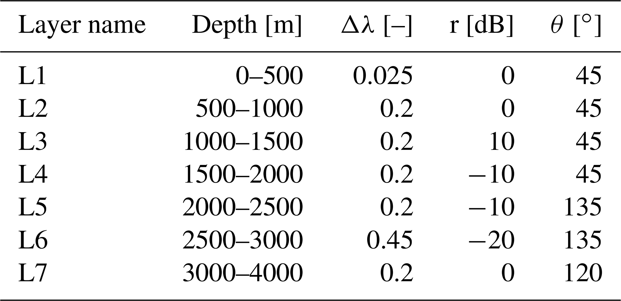
For a given depth profile of Δλ(z), θ(z), and r(z), the radar return can be simulated using the forward model described by Eqs. (4) and (5). We show a seven-layer synthetic model in Fig. 3 to visualize features in the radar data, which can be linked to ice fabric parameters. The model parameters used to generate Fig. 3 are shown in Table 2.
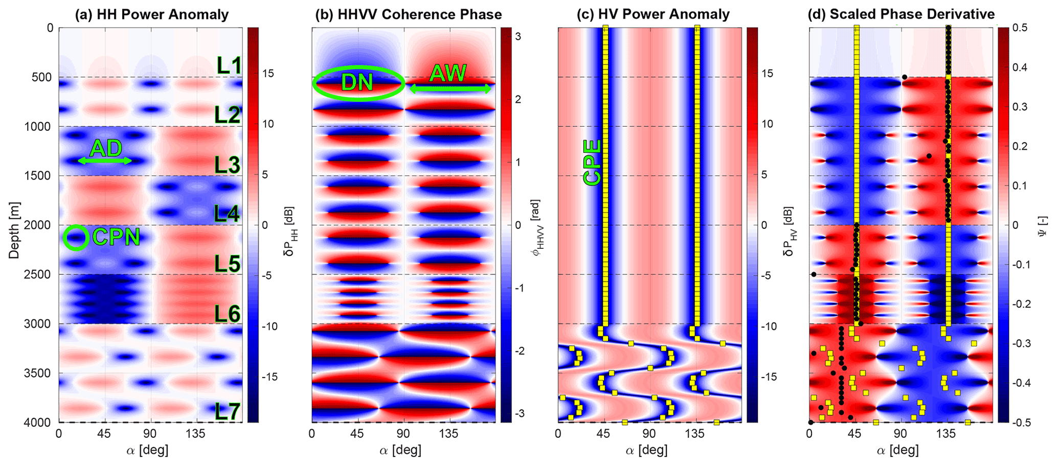
Figure 3A seven-layer synthetic model generated by Eq. (5) using the model parameters in Table 2. Horizontal dashed black lines are the layer boundaries with layer numbers from L1 to L7. (a) HH power anomaly (δPHH) representing co-polarization node (CPN) and node angular distance (AD). (b) HHVV coherence phase (ϕHHVV) displaying dipole co-polarized node (DN) and node angular width (AW). (c) HV power anomaly (δPHV) representing cross-polarization extinction (CPE). (d) Scaled phase gradient (Ψ) displaying the direction of v1 (yellow squares in blue areas) and v2 (yellow squares in red areas). The magnitude of Ψ at the black dots is the value of horizontal anisotropy (Δλ).
Power anomalies illustrate the effects of anisotropic ice
where is the amplitude of the complex received signal, and n is number of angular increments for θ. In δPHH, a number of co-polarization nodes (CPNs) occur, which result from destructive superposition of ordinary and extraordinary waves (Fig. 3a). The number of nodes per layer is only a function of ice fabric anisotropy in that layer, with higher horizontal anisotropy resulting in more nodes. The nodes occur at a variable angular distance (termed AD in Fig. 3a) if anisotropic reflection is relevant (e.g., L2 and L3 in Fig. 3a). The angular dependency of the co-polarization nodes on anisotropic scattering can be identified using a depth-invariant ice fabric orientation (constant θ). Previously, Fujita et al. (2006) approximated the correlation between AD and r with a linear regression. As detailed in Appendix F we improved this by finding the analytical solution
Differences in both approaches are illustrated in Fig. 4. Two important features in δPHH are therefore the frequency of occurrence of co-polarization nodes with depth (a first-order proxy for the horizontal anisotropy) and their angular distance (a mixed proxy for anisotropic reflections or depth-variable ice fabric orientation). δPHH can be 90∘ (e.g., L2) or 180∘ (e.g., L3) symmetric if rdB=0 or rdB≠0, respectively.
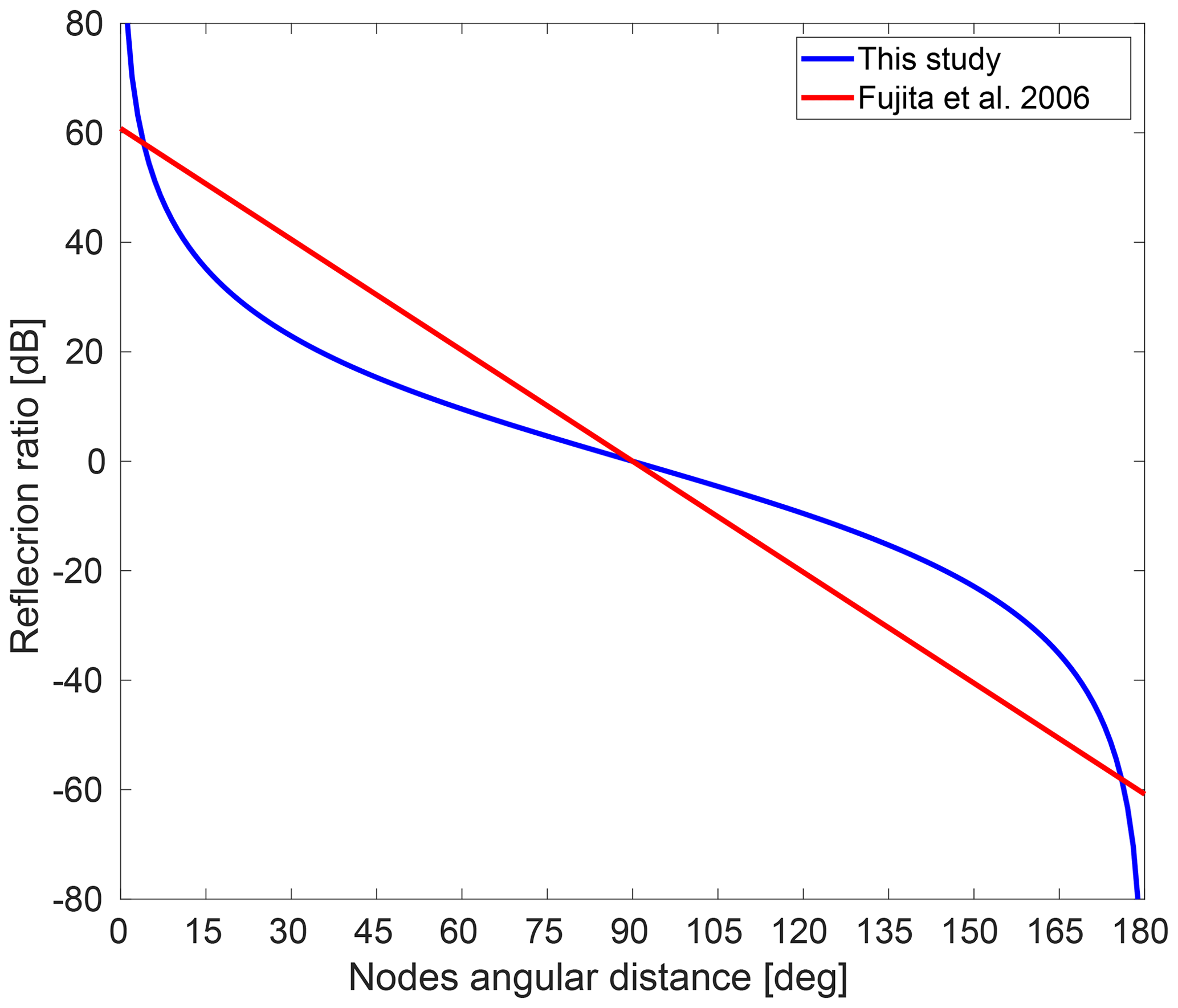
Figure 4Dependence of reflection ratio on the azimuthal difference between two nodes as determined by Fujita et al. (2006) and through Eq. (13).
In a depth-invariant ice fabric orientation, the minima in δPHV align with v1 and v2, termed cross-polarization extinction (CPE in Fig. 3c). Using the radar forward model, this can be derived analytically for a single-layer case as
where the solutions are at and . In multi-layer cases, where θ changes with depth (e.g., L6 and L7 in Fig. 3b), δPHV also depends on other parameters, making it difficult to infer θ using δPHV alone.
The co-polarization nodes in δPHH can also be observed in ϕHHVV (termed DN in Fig. 3b). The depth of the node can be automatically estimated at the zero-phase transition. Unlike δPHH, the nodes in ϕHHVV are 90∘ anti-symmetric, and their polarity is insensitive to r. This can be used to determine the directions of v1 and v2. The angular width of the nodes (termed AW in Fig. 3b) decreases when rdB≠0 (e.g., L3 or L4). The absolute value of Ψ at the principal axis's directions (v1 or v2) is a first-order proxy for Δλ at a given depth (Eq. 10, Fig. 3d). Since the scaled phase gradient (Fig. 3d) is anti-symmetric, and only the positive gradient is in the direction of v2, we mask negative parts of Ψ from now on.
3.5 An inverse approach to infer ice fabric from quad-polarimetric returns
Fujita et al. (2006) focused on the power anomalies from co- and cross-polarized measurements (δPHH, δPHV). Dall (2010) and Jordan et al. (2019) included the coherence phase gradient (Ψ) to quantify the ice fabric horizontal anisotropy (Δλ). However, particularly for multi-layer cases where the ice fabric parameters vary with depth, there has not yet been an established procedure for how ice fabric parameters can be reliably inverted from observations. Here, we use the previous work from Fujita et al. (2006), Dall (2010), and Jordan et al. (2019) and provide additional justification to infer all the ice fabric parameters in a continuous depth profile.
Our approach involves data preprocessing, initializing the model parameters, and parameter optimization using a constrained multivariable non-linear least-square inverse approach (Powell, 1983; Waltz et al., 2006). All the three eigenvalues are then estimated from the estimated Δλ and optimized r using a top-to-bottom, layer-by-layer approach assuming isotropic ice at the surface.
3.5.1 Data preprocessing
The full angular response is synthesized from HH, VV, and HV observations for a single TR orientation (θ) using Eq. (11) at 1∘ increments. The amount and method of smoothing applied to the data depend on nodes' vertical frequency and the phase polarity's sharpness. The power anomalies are smoothed by moving-average and 2D Gaussian convolution. The coherence phase (ϕHHVV) is inherently smoothed, depending on the size of the depth window in Eq. (7), while its gradient (Ψ) is smoothed with a 1D Gaussian convolution at each azimuth.
3.5.2 Model parameterization
We investigate two parameterization types for the free model parameters (θ, Δλ, r) with depth: piecewise constant and a superposition of Legendre polynomials. The former has the highest number of free model parameters but can capture abrupt variability with depth. The latter has a reduced set of free model parameters with improved performance during the inversion but varies more smoothly with depth. At Dome C, no abrupt variability is visible in the data so that we use the Legendre polynomials with 40 free model parameters (30 for θ, and 10 for r). At EDML, because of abrupt depth variability in r and θ, we default to the piecewise constant parameterization, resulting in 80 free model parameters (40 piecewise constant intervals at 50 m spacings for r and θ).
3.5.3 Derivation of initial guess
The non-linear optimization problem depends on a well-defined initial guess based on our inferences from the synthetic data. Initial guesses of variables are marked with superscript 0. We first derive the initial guess for the orientation of the ice fabric θ0(z) using the minima in δPHV, polarity in ϕHHVV, and the sign of Ψ. We then infer Δλ0(z) using the absolute value of Ψ at the minima of δPHV. The initial guess for is zero. The underlying assumption for all of the initial guesses is that θ does not vary significantly with depth.
3.5.4 Cost function and optimization
We optimize θ and r for all depth intervals, while at this stage we accept the estimated Δλ0 for horizontal anisotropy. There are a number of possible model data misfit metrics of power anomalies and phase differences,
and the total misfit between the observed (obs.) and the modeled data (mod.) is defined as
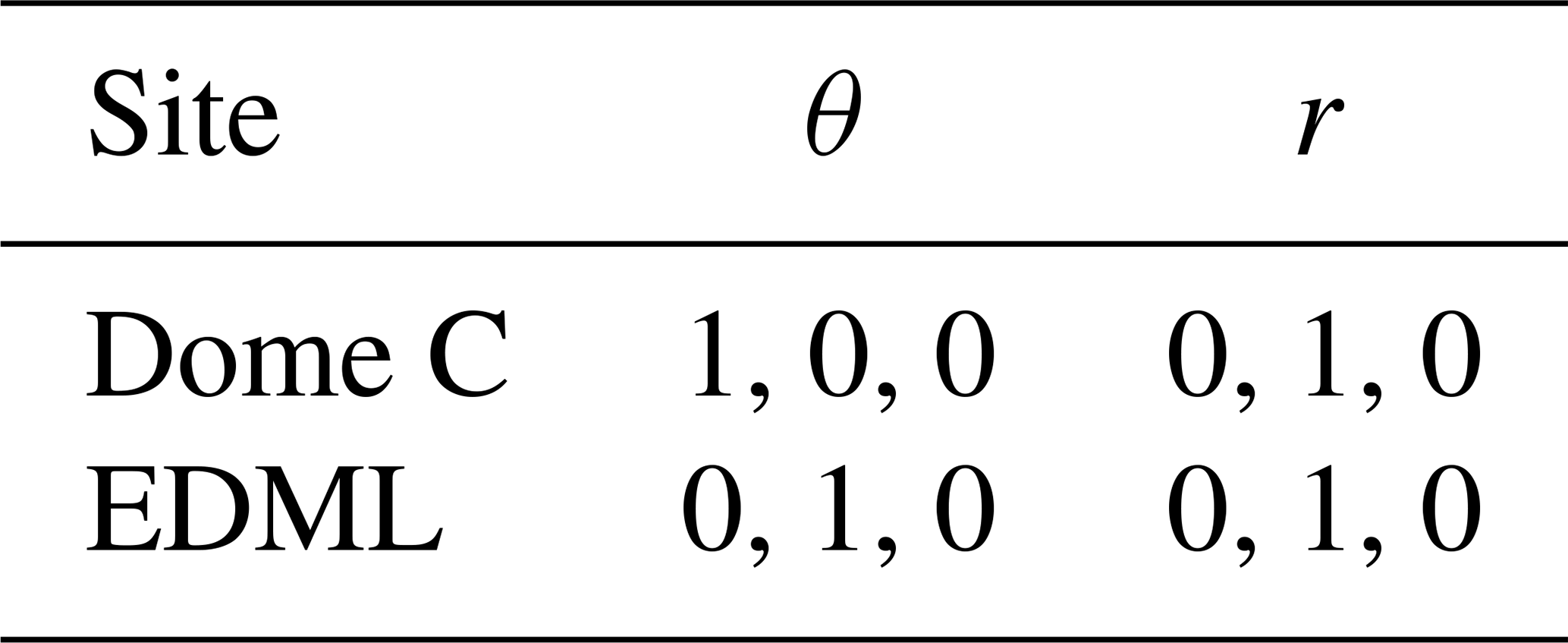
where l1, l2, and l3 are constants (0 or 1). Note that ϕ and δP in Eqs. (15) to (17) are standardized. In Table 3, we show the values of l1, l2, and l3 that we used for Dome C and EDML sites. The coherence phase misfit was not applicable in EDML due to strong ice fabric anisotropy. To further constrain the inversion, we set bounds on the model parameters so that , , and −30 dB 30 dB. This is implemented in the cost function in the form of log-barrier functions using MATLAB's fmincon algorithm.
Table 3The constant l1, l2, l3 for ice fabric parameters θ and r at Dome C and EDML.
3.6 Reconstruction of all eigenvalues
Once the radar forward model is optimized, we attempt to reconstruct all the three eigenvalues in a top-to-bottom approach. We use an additional assumption for the standard scattering model where the reflection coefficient can be described using the Fresnel equations (Paren, 1981; Drews et al., 2012). If anisotropic scattering is caused by depth-variable ice fabric, then the reflection ratio at the interfaces i and i+1 can be approximated by
Here, for the sake of simplicity, we only use the positive results for r. Solving Eq. (19) using the optimized r and Δλ can fully reconstruct λ1, λ2, and λ3 in a nadir geometry, which will resolve the ice fabric types' ambiguity, as explained in Appendix G. At the surface, ice is assumed to be isotropic (an assumption that we discuss later in Sect. 5.1) so that λ11≈0.33, allowing λ21 and λ31 to be inferred from the estimated Δλ1
The eigenvalues for the surface can be estimated by iterating through Eqs. (20) and (21) and decreasing the value of λ11 by at each iteration until all the surface eigenvalues fulfill the requirements in Sect. 3.1. For deeper layers i+1, all three eigenvalues can be reconstructed analytically by solving
for λ1i+1 and inferring λ2i+1 and λ3i+1 with
where Eq. (22) is a reformed version of Eq. (19). However, errors during the optimization may result in a reconstruction of the three eigenvalues, which do not comply with limits inferred in Sect. 3.1. In that case, Δλ and r are varied in a systematic search to find eigenvalues within the permissible limits. Solutions, in this case, are not unique, and additional constraints on the vertical gradients are required. Here, we use the vertical gradient between the two largest adjacent eigenvalues, where and . This correction does not significantly alter the results from the previous section but assures that the inferred eigenvalues are internally consistent.
4.1 Ice fabric parameters from polarimetric ApRES at EDC
Polarimetric ApRES data collected at EDC are shown in Fig. 5a–d. A co-polarization node occurs at 1100 m depth, and a second node develops at about 2000 m depth (Fig. 5a, b). The existence of only one pair of nodes over 2000 m indicates comparatively small horizontal ice anisotropy (i.e., low Δλ), similar to what has been observed at Dome Fuji (Fujita et al., 2006). The angular distance between the two co-polarization nodes is close to 90∘, consistent with r close to 0 dB (Fig. 5a). δPHV shows little depth variability (Fig. 5c), suggesting that the ice fabric orientation angle (θ) does not vary strongly with depth. The scaled phase derivative (Ψ, Fig. 5d) is unclear in terms of polarity for the top 150 m. Below that, the polarity more clearly indicates the orientation of the largest horizontal eigenvectors.
Optimized model results in Fig. 5e–h reproduce the principal patterns of the radar observations. The reconstructed eigenvalues (Fig. 5i) capture the observed transition from isotropic to a girdle-type ice fabric in the ice core data. The reconstructed horizontal anisotropy (Fig. 5j) captures the mean well (), albeit showing less depth variability than the observations. Note that there is no significant change in the eigenvalues and horizontal anisotropy at a depth of the node's occurrence since the node's depth depends on the integration of the horizontal anisotropy above that depth and not at that depth. The ice fabric orientation at the top 150 m is poorly constrained due to the low horizontal anisotropy (Fig. 5k). The mean orientation of v2 below 150 m is 124∘ relative to true north, which is almost perpendicular to the surface flow direction towards 45∘. The orientation cannot be validated with ice core data, which is azimuthally unconstrained. The mean estimated reflection ratio below 150 m is low ( dB, Fig. 5l), indicating that the role of anisotropic reflections is small.
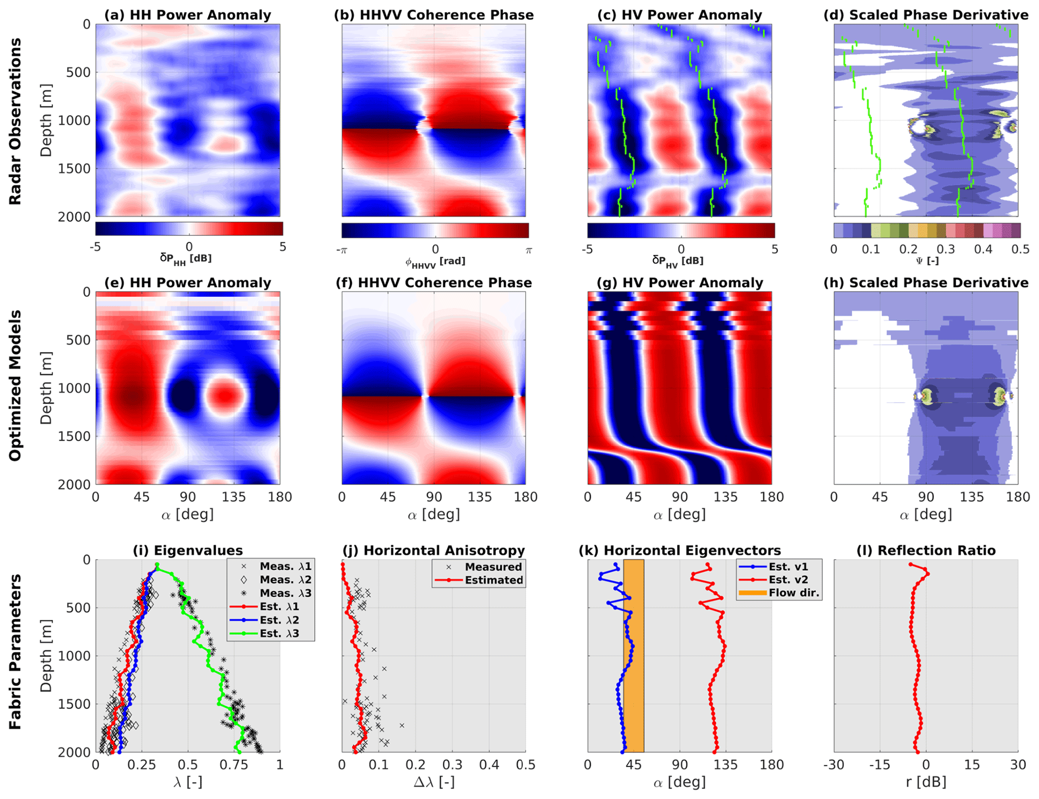
Figure 5Results for EDC: (a)–(d) radar observations, with green lines in (c) and (d) marking the minima in δPHV. (e)–(h) Optimized model output capturing the principle patterns of the observations. (i)–(l) Inferred model parameters validated with ice core data (Durand et al., 2009) in terms of eigenvalues (i) and horizontal anisotropy (j). The inferred v2 is perpendicular to the mean surface flow direction (k), and the anisotropic reflection ratio is small (l). Note that the negative Ψ values in (d) and (h) are masked for a better demonstration of v2 orientation.
4.2 Ice fabric parameters from polarimetric ApRES at EDML
Next, we apply the inverse approach to ApRES data collected at the EDML drill site. Contrary to what has been observed at EDC, co-polarization nodes can barely be localized in δPHH as no 90∘ symmetry is apparent (Fig. 6a). This indicates that anisotropic scattering is relevant (r≠0 dB), as already noticed earlier (Drews et al., 2012). Moreover, the coherence phase shows many nodes (Fig. 6b), indicating a much stronger horizontal anisotropy (i.e., large Δλ). This is comparable to the ice core at Mizuho, equally located in a flank flow regime (Fujita et al., 2006). Although δPHV shows almost no depth variability in ice fabric orientation (Fig. 6c), it is not straightforward to identify the direction of v1 and v2 using the polarity of Ψ because of the strong ice anisotropy (Fig. 6d).
The optimized model (Fig. 6e–h) reproduces all basic features seen in the radar data. Inferred model parameters closely follow the ice core measurements both in terms of absolute eigenvalues (Fig. 6i) and horizontal anisotropy (Fig. 6j). A shallower development of the girdle ice fabric compared to EDC is detected. At this site, the mean ice fabric anisotropy at the top 200 m is weak, but in comparison to EDC it is strong enough to detect the ice fabric orientation. The mean estimated horizontal anisotropy below 200 m in EDML () is more than 7 times stronger than EDC. The mean inferred orientation of v2 below 200 m is 174∘ relative to true north (Fig. 6k). Similar to EDC, this is near-perpendicular to the ice flow direction at the surface towards 90∘. The estimated reflection ratio in EDML (Fig. 6l) can be divided into two major zones ( dB, and dB). Contrary to EDC, anisotropic reflections are more relevant, and the previously suggested existence of two anisotropic scattering zones above and below approx. 850 m (Drews et al., 2012) appears in the observations and the optimized model output.
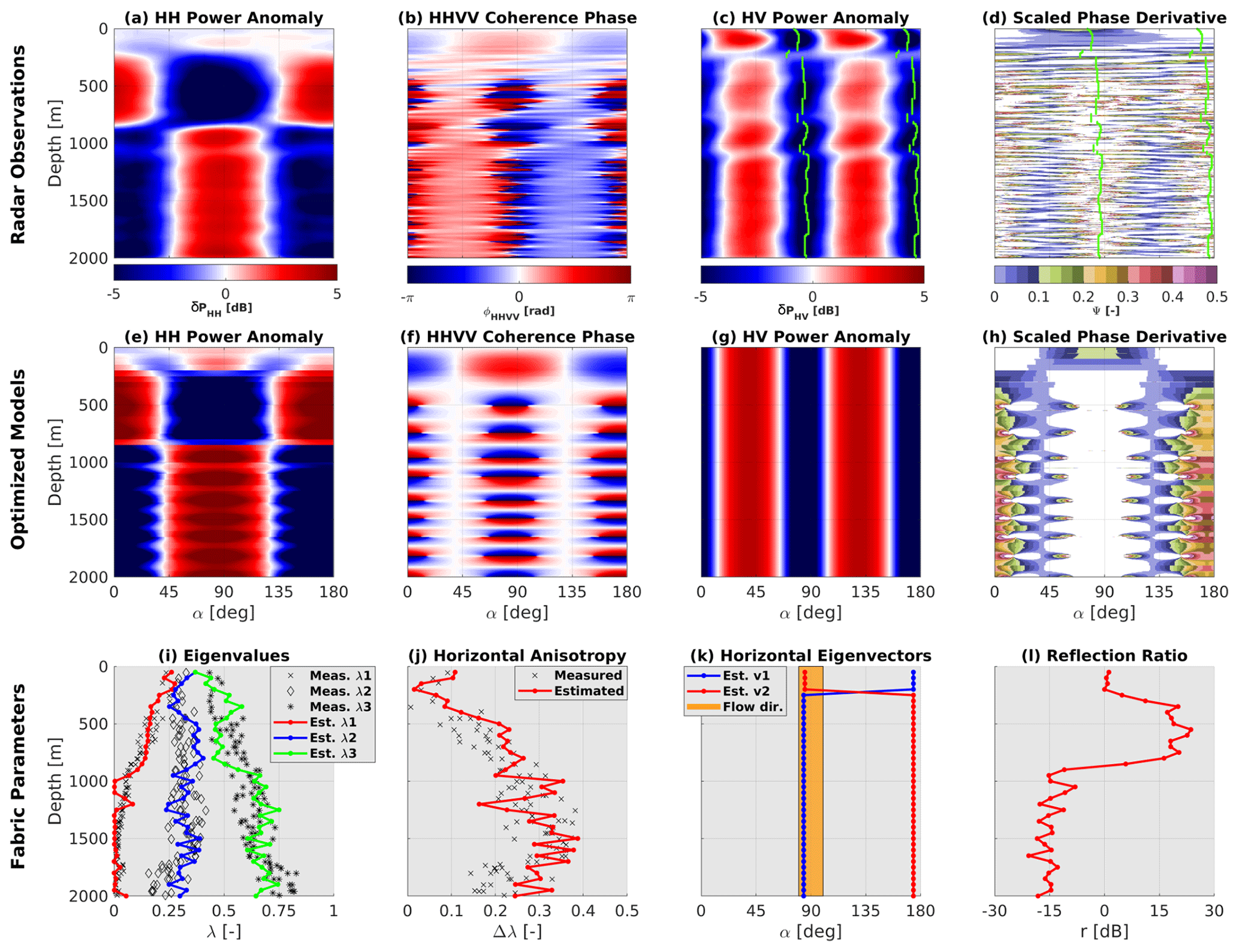
Figure 6Results for EDML: same as Fig. 5, with the exception that the measured parameters in (i) and (j) are from Weikusat et al. (2017).
4.3 Spatial variability in ice fabric parameters in the local dome–flank transition zone
After investigating specific characteristics of a dome position (EDC) and a flank-flow regime (EDML), we next investigate a local dome-to-flank transition (36 km). At Dome C, 19 sites are located along a profile extending 18 km away to either side from the local ice dome (Fig. 1a), and a summary of the results is presented in Fig. 7. We focus on the upper 2000 m, where the signal-to-noise ratio and the coherence magnitude are sufficiently high. All stations yield coherent results, showing an isotropic ice fabric that gradually evolves into a weak girdle with depth. The depths of the first co-polarization nodes can be detected at all sites (dashed green line in Fig. 7b). It is shallowest beneath the dome and moves to larger depths further away from the dome in the flanks. The depth variability in the co-polarization nodes results in a Δλ that is most anisotropic beneath the dome and less anisotropic in the flanks (Fig. 7c). The orientation of the eigenvectors is poorly constrained in the upper 200 m. At larger depths, they are oriented parallel (v1) and perpendicular (v2) to the surface flow direction, in line with what is inferred in Sect. 4.1.
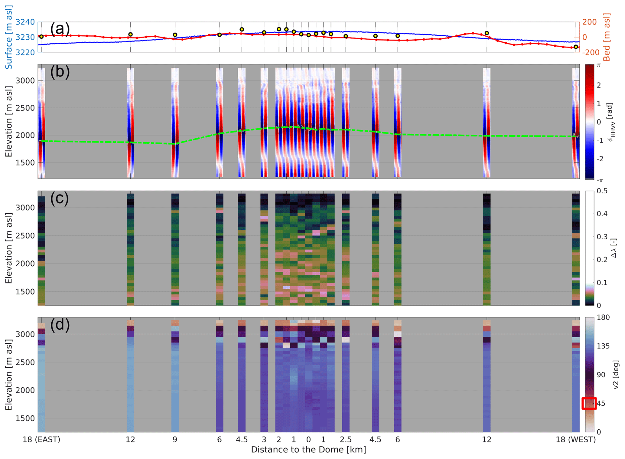
Figure 7Ice fabric evolution in the local dome-to-flank transition at Dome C. (a) Surface (Howat et al., 2019) and bed (Morlighem et al., 2020) elevation in meters above sea level. Yellow circles are the measured bed elevation from radar power return at each site. (b) Observed polarimetric coherence phase difference (ϕHHVV) at each site. The dashed green line connects the nodes at each site. (c) The optimized horizontal anisotropy (Δλ). (d) The optimized orientation of the largest horizontal eigenvector (v2). The red rectangle in the legend marks the surface flow direction. All panels are corrected for the surface elevation, i.e., statically corrected.
5.1 Radar polarimetry as a tool to characterize ice fabric variability horizontally and vertically
The method we developed in this study extracts the depth variability in ice fabric horizontal anisotropy (Δλ) and anisotropic reflection ratio (r), which leads to estimating all three eigenvalues required for the second-order ice fabric orientation tensor. We also estimate the georeferenced ice fabric orientation (v2) as a function of depth. The results of our method are comparable with laboratory measurements (Durand et al., 2009; Weikusat et al., 2017) and could be integrated into anisotropic ice flow models (Azuma, 1994; Azuma and Goto-Azuma, 1996; Gagliardini et al., 2009). Our main assumption is that the strongest eigenvector (and with it the orientation tensor) is aligned in the vertical.
In terms of the data preprocessing, there are no structural differences in our data between synthesizing the polarization dependency out of a single set of quad-polarimetric measurements (Appendix E) and the more common polarimetric measurements in glaciology, where antennas are kept parallel or perpendicular while being rotated several increments between 0 and 180∘ (Fujita et al., 2006). In addition to significantly reducing the field time for data acquisition, an advantage of these measurements is that the georeferencing error only occurs once during antenna setup and is not accumulated over multiple re-positioning cycles. However, it is required that the data have a sufficiently high signal-to-noise ratio (e.g., using ) in order to not synthesize misleading symmetries out of noise.
The signal quality and noise level, particularly in the HHVV coherence phase, are important. In areas with high horizontal anisotropy and consequently densely spaced co- and cross-polarization nodes (i.e., the EDML case), care needs to be taken that the denoising does not average over multiple nodes. Derivation of the initial guess for the inverse approach depends on the data quality and is guided by characteristic features in synthetic forward models, some of which can be analytically described for one-layer cases. Multi-layer cases, however, are difficult to interpret, particularly if the ice fabric orientation (v2) changes strongly (by several tens of degrees) with depth (e.g., ice shelves and glaciers). Fortunately, this does not appear to be the case for the data presented here (Figs. 5k, 6k) so that the initial guess already results in a forward model that adequately captures characteristic features in the data. The optimization improves the model–data misfit but does not lead to significant differences with our first informed guess. Nevertheless, this step is required to predict the depth variability in all the three eigenvalues (Sect. 3.6).
The reconstruction of the eigenvalues assumes isotropic ice and firn for the surface (λ1=0.33). This is reasonable for the dome and flank-flow settings considered here but may need to be revisited in other settings where ice fabric can develop near the surface as ice streams and ice shelves. More critical is the reflection ratio itself, which is ill-constrained in magnitude and amplifies small changes in the eigenvalues across the reflection boundaries. This is mitigated by the range of allowed eigenvalues (Sect. 3.1), and it is those constraints that facilitate the derivation of all eigenvalues from the anisotropic reflection ratio. The predicted eigenvalues (λ1, λ2, and λ3) in this method show a good match to the ice core observations in both cases.
The azimuthal constraints that radar polarimetry provides can, in general, not be validated by ice core measurements, with few exceptions (e.g., Westhoff et al., 2020). However, the alignment of the ice fabric principal axes with the surface-flow direction detailed below adds credibility to our inferences and shows advantages of this approach over previous attempts focusing on the power anomalies only (Fujita et al., 2006; Matsuoka et al., 2012). The underlying reason for this is that the polarity of the depth gradient of the polarimetric coherence phase is independent of anisotropic scattering.
The inversion requires an initial guess (Sect. 3.5.3) that is based on experience from synthetic test cases. In our experience with radar polarimetry and the explored ice dynamic context, this grants a robust solution, also because a wrong initial guess results in a large model–data misfit that can be identified easily. In the future, this can be improved by using gradient-free optimization schemes (e.g., in a Bayesian framework) that can correct for a poor initial guess by exploring the parameter space more systematically.
Our strongest assumption is that the strongest eigenvector (v3) should be close to vertical. While this assumption is justified here, as flow at domes is dominated by vertical compression, and the crystal c axis tends to be aligned in the vertical, it may not apply elsewhere in ice sheets and cause an additional source of horizontal birefringence (Matsuoka et al., 2009). While it is possible to explore other effects than that of the largest eigenvector being vertical (Jordan et al., 2019, p. 13), it is impossible to circumvent the fact that the radio wave propagation is vertical and hence insensitive to changes along that direction. In the future, we envision the use of wide-angle surveys with curved ray paths (e.g., Winebrenner et al., 2003) to overcome this limitation.
With the assumptions mentioned above, radar polarimetry is now a step closer to constrain the second-order orientation tensor. However, this is still not the full representation required to characterize all ice fabric types, for example because a strong vertical girdle and weak horizontal cones will have a similar second-order orientation tensor. A combination with seismic studies recovering the fourth-order elasticity tensor (Diez and Eisen, 2015; Diez et al., 2015) is therefore still warranted.
5.2 Spatial variability in ice fabric types in dome–flank transitions
We now investigate our inferred characteristics of ice fabric variation at the dome, where flow is dominated by vertical compression, compared with the flanks, where flow is dominated by vertical shear. Our inverse approach shows higher horizontal ice anisotropy at EDML compared to Dome C throughout the ice column. This increase from the dome to the flank supports earlier inferences that ice anisotropy is larger in areas with significant horizontal strain compared to settings where vertical compression is dominant (Fujita et al., 2006; Matsuoka et al., 2012). This is in contrast, however, with the observed decrease in ice anisotropy in the Dome C transect (Fig. 7c), where the ice fabric is more anisotropic at the Dome compared to the flanks. Our hypothesis is that this near-field anomaly reflects ice dynamic modification of ice fabric through the Raymond effect (Raymond, 1983). Martín et al. (2009) predict local ice-dynamically induced ice fabric variability up to approximately five ice thicknesses to either side of ice divides. The 36 km long Dome C transect images an ice thickness of about 3000 m and hence approximately covers this domain. The absence of Raymond arches in the radar stratigraphy beneath Dome C (Cavitte et al., 2016) suggests that these need a longer time to evolve, whereas the ice fabric pattern likely reflects the instantaneous operation of the Raymond effect. We acknowledge that there are other explanations for the ice fabric pattern under Dome C, such as across-profile flow or bedrock influence. In any case, we want to highlight here how, due to the spatial extension of our observations, our inferred ice fabric distributions combined with an anisotropic flow model can be used to test these and other hypotheses.
Focusing on the top 200 m of the inferred Δλ and v2 reveals a significant difference between the two sites. At EDML, the ice fabric anisotropy is stronger in the top 200 m, resulting in a better-constrained ice fabric orientation, whereas at EDC it is entirely unconstrained (Figs. 5d and 6d). It appears that the ice fabric orientation develops more rapidly in areas with significant horizontal flow compared to areas with essentially vertical compression only.
In both the EDML and Dome C areas, the inferred ice fabric orientation varies little over the depth intervals considered, and in both cases, the inferred orientations line up with the surface flow field. More specifically, v1 is approximately oriented along-flow, and v2 is approximately oriented across-flow. Those directions also align with the principal strain rate components (Fig. 1) in Dome C (Rémy and Tabacco, 2000; Vittuari et al., 2004) and EDML (Drews et al., 2012). In both cases, v2 is approximately parallel to the direction of the maximal principal strain rate component, whereas v1 is aligned with the along-flow minimal principal strain rate component. At Dome C, where ice flow velocities are low, derivation of the strain rate field is not trivial and adds additional assumptions of the surface topography (Vittuari et al., 2004). Note that ice is compressing in the direction of flow and not extending, as is often assumed in simplified theoretical examples, which is why it is important to reference the ice fabric to the direction of extension and compression and not the flow.
The origin of the difference in radar polarimetry between EDC and EDML is the degree of ice fabric alignment in the horizontal, which can be quantified as the difference between the horizontal eigenvalues of the orientation tensor. This difference is larger for EDML than for EDC. Our study adds to the body of evidence that ice fabric is induced by flow because the preferred direction for horizontal ice fabric aligns with the direction of compression (Drews et al., 2012). In addition, the stronger horizontal alignment of the ice fabric at EDML, compared to EDC, corresponds to a stronger compression that can be observed by comparing the strain ellipses in Fig. 1. It is interesting to notice how sensitive radar polarimetry is to horizontal ice fabric alignment, the main observable for downward-looking radar. Despite the small differences in horizontal ice fabric eigenvalues at EDC (Δλ<0.05 in Fig. 5j) our technique is able to recover ice fabric in most of the column. This is of particular interest as the ice fabric could contain a record of past changes in ice flow conditions (Brisbourne et al., 2019).
More theoretical work is required to understand the vertical variability in horizontal anisotropy, which is picked up in radar polarimetry through the strength of the anisotropic reflection ratio. At EDML, the reflection ratio is a dominant and required factor to explain the radar signatures, while at Dome C, it is close to negligible. Fujita et al. (2006) have observed a similar increase in anisotropic scattering between Dome F and Mizuho, suggesting that this may be a generic feature in ice sheets that requires more investigation. Contrary to EDML, the signal at Dome C is dominated by birefringence, and the contribution of anisotropic reflection is small. Yet, it appears that it leaves a small signature in the data that can be detected. Moreover, our analysis suggests that there are no other mechanisms (e.g., a directional interface roughness) contributing to anisotropic reflections. This point requires confirmation from other ice core sites because the recovery of all three eigenvalues (and their corresponding directions) offers significant possibilities of constraining ice fabric in ice sheets in general.
Although anisotropic reflections at Dome C are small, there is a noticeable change in the δPHH of direction in the depth interval from 1500–1700 m, which coincides with the transition from Holocene to glacial ice, as is also the case for the EDML site (Drews et al., 2012). The inversion does not pick up this feature in r as it is at the boundary of the domain (Fig. 5l), and we do not have a complete understanding why glacial–interglacial transitions should be accompanied by changing reflection ratios. Nevertheless, this may provide us with an additional tool to explore age–depth relationships at future ice core sites.
We show here the spatial distribution of ice fabric in domes: from the summit, where flow is dominated by vertical compression, to the flanks, where flow is driven by vertical shear. The combination of co- and cross-polarized power anomaly along with the depth gradient of polarimetric coherence phase provides three major parameters and their changes over depth, i.e., the ice fabric orientation, horizontal anisotropy, and its vertical variability. We quantify these changes using an inverse approach that extracts ice fabric information from radar polarimetry. Our method approximates the full orientation tensor including the vertical ice anisotropy. This information can be used in the future to better understand, for example, how susceptible the ice is to shearing within the ice column (Azuma and Goto-Azuma, 1996). We validate our technique with data from two ice core locations situated in contrasting ice flow regimes. The inferred ice fabric orientation aligns with the observed surface velocity and surface strain rate fields. This suggests that polarimetric radar is an ideal tool to map ice fabric characteristics elsewhere as well.
We present ice fabric spatial distribution across a flow plane at Dome C. The 20 ApRES sites in that area are internally consistent, and small changes in the horizontal anisotropy can be horizontally tracked in the polarimetric coherence phase. We detect a minor decrease in horizontal anisotropy away from the dome that we tentatively link to the operation of the Raymond effect. On larger spatial scales, the horizontal anisotropy increases in the flanks (i.e., at EDML), and our findings are consistent with previous studies. Our analysis suggests that ice fabric characteristics can now be reliably inferred in larger parts of Antarctica and the Greenland ice sheet, given that more and more profiles are recorded in a quad-polarimetric configuration. This will be a decisive step to further constrain the anisotropic nature of ice and better understand its contribution to internal deformation.
Table A1ApRES stations info. Coordinates are shown in decimal degrees in the WGS84 reference system. Surface elevations are extracted from the Reference Elevation Model of Antarctica (REMA; Howat et al., 2019). Bed elevations are obtained from the polarimetric-radar data. Tx–Rx azimuth is measured by a compass with tolerance.
Here, we briefly explain the parameters from Eq. (5). The depth factor in this equation is
where j is the imaginary unit, and is the wavenumber in a vacuum, with c0 the speed of light in a vacuum.
The transmission of the signal is described by the transmission matrix T along the ice fabric horizontal principal axes. T is a function of wavenumbers kx and ky, whereas the wavenumbers can be expressed as a function of dielectric permittivities (, ) and electrical conductivities (σx, σy) (Fujita et al., 2006).
where ε0 and μ0 are the dielectric permittivity in a vacuum and the magnetic permeability in a vacuum, respectively, and ω is the angular frequency. In this study we follow Ackley and Keliher (1979) and Fujita et al. (2006) and assume isotropicelectrical conductivity (σx=σy). Using Eq. (3), T can be written as a function of eigenvalues
where it tracks the relative phase shifts induced by the dielectric anisotropy along the ice fabric principal axes. The reflection matrix Γ describes the reflection of the radio waves at an interface with changing dielectric properties
A rotation between the TR aerial line and v1 of the ice fabric in layer i is accounted for by the rotation matrix R and its transpose (R′):
Here we expand individual components of a single-layer case that are used later to determine the relationship between the anisotropic reflection ratio and the angular distance of the co-polarization nodes. For this case, we drop the indices relating to the different layers and expand Eq. (5):
so that
The complex sHH, its amplitude, and its phase are then
respectively. Also, the complex sHV, its amplitude, and its phase, respectively, are
This section details the relationship between the polarity of the phase gradient and the corresponding directions of the eigenvectors. Care has to be taken here as the deramping during ApRES data acquisition is equivalent to a complex conjugation of the received signal. If this is not accounted for, the inferred eigenvector v1 and v2 will be swapped. More specifically, for a received signal at ,
so that the coherence phase results in
and conversely for
As explained in Appendix B, kx and ky are a function of λ1 and λ2, respectively. Because λ1≤λ2 it follows that kx<ky. Therefore, and . The reverse holds for .
The transformation is purely geometrical and corresponds to a coordinate transformation into a rotated reference system for an arbitrary γ:
resulting in
Figure E1 demonstrates this approach for the EDML site, where quad-polarimetric measurements were additionally complemented by a dataset collected with rotating antennas. There are no structural differences between both datasets.
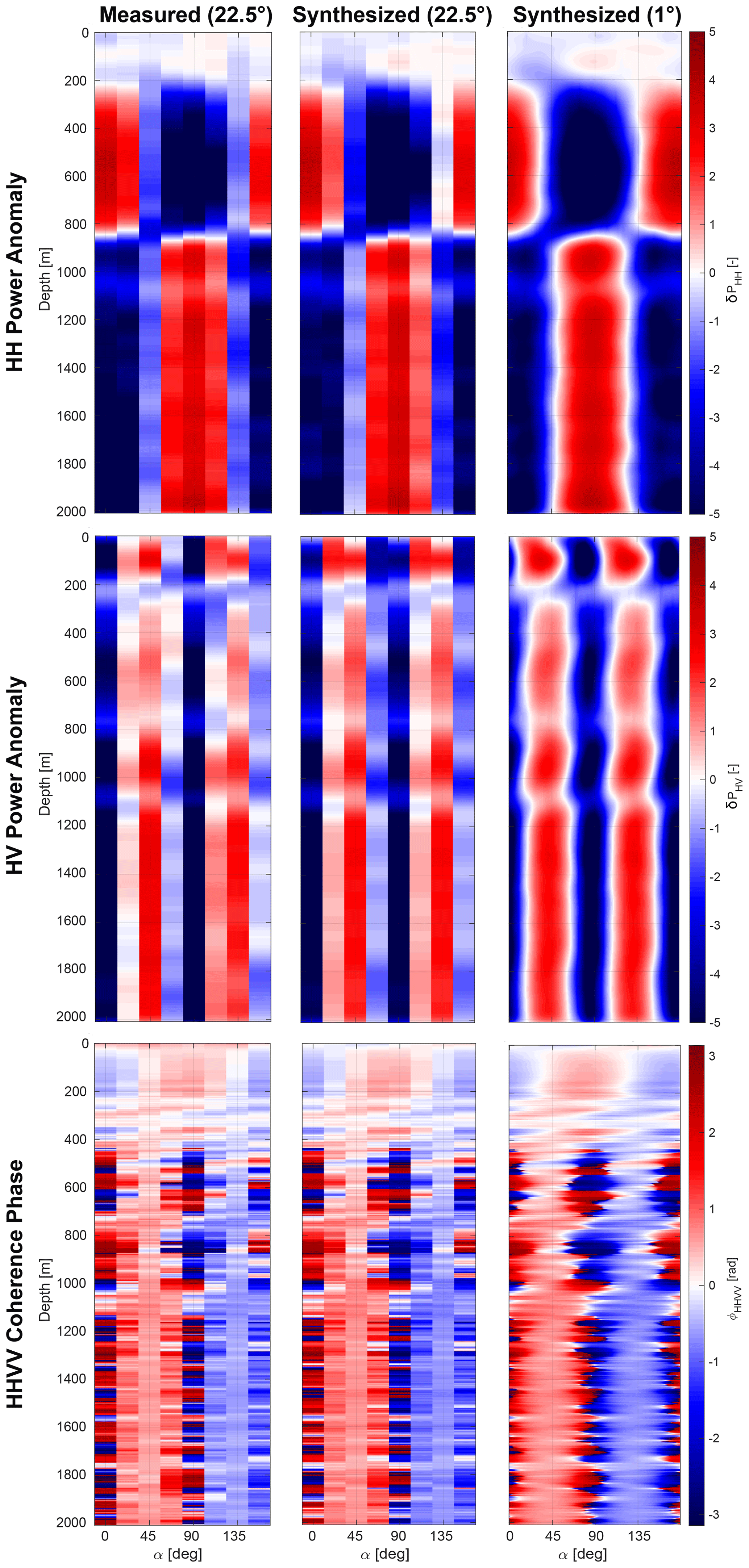
Figure E1Comparison between measured and synthesized ApRES data at the EDML site. Left column: measured ApRES data (22.5∘ azimuthal spacing). Middle column: synthesized ApRES data (22.5∘ azimuthal spacing). Right column: synthesized ApRES data (1∘ azimuthal spacing).
Here, we quantify the angular distance of co-polarization nodes (AD) as a function of the anisotropic reflection ratio (r). This defaults to a two-dimensional minimization problem in z and θ in the power anomaly δPHH. A co-polarization node in Eq. (C6) requires
The remaining quadratic equation has two solutions corresponding to the two co-polarization nodes:
The angular distance between these nodes then results in
which can be rearranged for the reflection ratio as
Since polarimetric radar is insensitive to the vertical component of the ice fabric, it is only possible to estimate its horizontal anisotropy from the matrix model alone (Sect. 3.3). As shown in Fig. G1, the value of is not sufficient to infer the ice fabric type. End-member cases in Fig. G1a–c are the values for λ1, λ2, and λ3 for an isotropic (I), single-pole maximum (S), and girdle-type (G) ice fabric. Although the uncertainty in detecting the ice fabric type decreases for stronger Δλ, to constrain the ice fabric type from the polarimetric radar, all three eigenvalues along the ice fabric principal axes are necessary. The triangular shape of Fig. G1 is due to the constraints on the λ1, λ2, and λ3 values, as mentioned in Sect. 3.1.
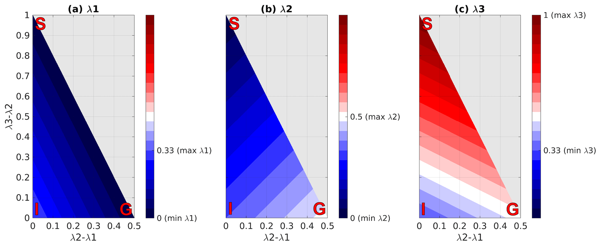
Figure G1Ice fabric type and eigenvalue (a) λ1, (b) λ2, and (c) λ3 as a function of eigenvalue differences λ2−λ1 and λ3−λ2. (I) isotropic ice fabric where λ2−λ1 and . (S) Single-pole maximum ice fabric where and . (G) Vertical girdle ice fabric where and .
The entire code was written by the author and is publicly available on GitHub (https://github.com/RezaErshadi/ApRES_InverseApproach, last access: 19 April 2022; DOI: https://doi.org/10.5281/zenodo.4447487; Ershadi, 2021).
EDML radar data are cited as Christmann et al. (2020); DOI: https://doi.org/10.1594/PANGAEA.913719. Dome C radar data are cited as Corr et al. (2021); DOI: https://doi.org/10.5285/634EE206-258F-4B47-9237-EFFF4EF9EEDD.
MRE led the code development and writing of the manuscript. RD, CM, and OE designed the study outline. RM, CR, and HC led the quad-polarimetric acquisition scheme and data collection at Dome C. JC, OZ, and AH led data acquisition at EDML. All authors contributed to the writing of the final paper.
At least one of the (co-)authors is a member of the editorial board of The Cryosphere. The peer-review process was guided by an independent editor, and the authors also have no other competing interests to declare.
Publisher’s note: Copernicus Publications remains neutral with regard to jurisdictional claims in published maps and institutional affiliations.
M. Reza Ershadi and Reinhard Drews were supported by a DFG Emmy Noether grant (grant no. DR 822/3-1). This publication was also generated in the frame of Beyond EPICA Oldest Ice. The project has received funding from the European Union’s Horizon 2020 research and innovation program under grant agreement nos. 815384 (Oldest Ice Core) and 730258 (CSA). It is supported by national partners and funding agencies in Belgium, Denmark, France, Germany, Italy, Norway, Sweden, Switzerland, the Netherlands, and the United Kingdom. The Dome C measurements were made possible by the logistics provided by IPEV (prog. 902) and PNRA. We thank Luca Vittuari (University of Bologna, Italy) for the positioning of the stakes. The opinions expressed and arguments employed herein do not necessarily reflect the official views of the European Union funding agency or other national funding bodies. This is Beyond EPICA publication number 25. We thank the AWI logistics personnel for support of the work at Kohnen, made available through Alfred-Wegener-Institut Helmholtz-Zentrum für Polar- und Meeresforschung (2016).
This research has been supported by the Deutsche Forschungsgemeinschaft (grant no. DR 822/3-1) and the Horizon 2020 research and innovation program and coordination and support action (Beyond EPICA (grant no. 815384) and BE-OI (grant no. 730258)).
This open-access publication was funded by the University of Tübingen.
This paper was edited by Adam Booth and reviewed by Thomas Jordan, Emma C. Smith, and one anonymous referee.
Ackley, S. F. and Keliher, T. E.: Ice sheet internal radio-echo reflections and associated physical property changes with depth, J. Geophys. Res., 84, 5675–5680, https://doi.org/10.1029/JB084iB10p05675, 1979. a, b
Alfred-Wegener-Institut Helmholtz-Zentrum für Polar- und Meeresforschung: Neumayer III and Kohnen Station in Antarctica operated by the Alfred Wegener Institute, Journal of large-scale research facilities, 2, A85, https://doi.org/10.17815/jlsrf-2-152, 2016. a
Azuma, N.: A flow law for anisotropic ice and its application to ice sheets, Earth Planet. Sc. Lett., 128, 601–614, https://doi.org/10.1016/0012-821X(94)90173-2, 1994. a, b
Azuma, N. and Goto-Azuma, K.: An anisotropic flow law for ice-sheet ice and its implications, Ann. Glaciol., 23, 202–208, https://doi.org/10.3189/S0260305500013458, 1996. a, b
Bohleber, P., Wagner, N., and Eisen, O.: Permittivity of ice at radio frequencies: Part II. Artificial and natural polycrystalline ice, Cold Reg. Sci. Technol., 83–84, 13–19, https://doi.org/10.1016/j.coldregions.2012.05.010, 2012. a
Brennan, P. V., Nicholls, K., Lok, L. B., and Corr, H.: Phase-sensitive FMCW radar system for high-precision Antarctic ice shelf profile monitoring, IET Radar, Sonar & Navigation, 8, 776–786, https://doi.org/10.1049/iet-rsn.2013.0053, 2014. a, b, c
Brisbourne, A. M., Martín, C., Smith, A. M., Baird, A. F., Kendall, J. M., and Kingslake, J.: Constraining Recent Ice Flow History at Korff Ice Rise, West Antarctica, Using Radar and Seismic Measurements of Ice Fabric, J. Geophys. Res.-Earth, 124, 175–194, https://doi.org/10.1029/2018JF004776, 2019. a, b, c, d
Cavitte, M. G. P., Blankenship, D. D., Young, D. A., Schroeder, D. M., Parrenin, F., Lemeur, E., Macgregor, J. A., and Siegert, M. J.: Deep radiostratigraphy of the East Antarctic plateau: connecting the Dome C and Vostok ice core sites, J. Glaciol., 62, 323–334, https://doi.org/10.1017/jog.2016.11, 2016. a
Chartrand, R.: Numerical Differentiation of Noisy, Nonsmooth Data, ISRN Applied Mathematics, 2011, 164564, https://doi.org/10.5402/2011/164564, 2011. a
Christmann, J., Zeising, O., and Humbert, A.: Polarimetric phase-sensitive Radio Echo Sounder measurements at EDML, 2017, PANGAEA [data set], https://doi.org/10.1594/PANGAEA.913719, 2020. a
Cook, S. J., Swift, D. A., Kirkbride, M. P., Knight, P. G., and Waller, R. I.: The empirical basis for modelling glacial erosion rates, Nat. Commun., 11, 759, https://doi.org/10.1038/s41467-020-14583-8, 2020. a
Corr, H., Ritz, C., and Martin, C.: Polarimetric ApRES data on a profile across Dome C, East Antarctica, 2013–2014, British Antarctic Survey [data set], https://doi.org/10.5285/634EE206-258F-4B47-9237-EFFF4EF9EEDD, 2021. a
Dall, J.: Ice sheet anisotropy measured with polarimetric ice sounding radar, in: 2010 IEEE International Geoscience and Remote Sensing Symposium, Honolulu, HI, USA, 25–30 July 2010, pp. 2507–2510, https://doi.org/10.1109/IGARSS.2010.5653528, 2010. a, b, c, d
Diez, A. and Eisen, O.: Seismic wave propagation in anisotropic ice – Part 1: Elasticity tensor and derived quantities from ice-core properties, The Cryosphere, 9, 367–384, https://doi.org/10.5194/tc-9-367-2015, 2015. a, b
Diez, A., Eisen, O., Hofstede, C., Lambrecht, A., Mayer, C., Miller, H., Steinhage, D., Binder, T., and Weikusat, I.: Seismic wave propagation in anisotropic ice – Part 2: Effects of crystal anisotropy in geophysical data, The Cryosphere, 9, 385–398, https://doi.org/10.5194/tc-9-385-2015, 2015. a, b
Doake, C. S. M., Corr, H. F. J., and Jenkins, A.: Polarization of radio waves transmitted through Antarctic ice shelves, Ann. Glaciol., 34, 165–170, https://doi.org/10.3189/172756402781817572, 2002. a
Drews, R., Eisen, O., Steinhage, D., Weikusat, I., Kipfstuhl, S., and Wilhelms, F.: Potential mechanisms for anisotropy in ice-penetrating radar data, J. Glaciol., 58, 613–624, https://doi.org/10.3189/2012JoG11J114, 2012. a, b, c, d, e, f, g
Drews, R., Matsuoka, K., Martín, C., Callens, D., Bergeot, N., and Pattyn, F.: Evolution of Derwael Ice Rise in Dronning Maud Land, Antarctica, over the last millennia, J. Geophys. Res.-Earth, 120, 564–579, https://doi.org/10.1002/2014JF003246, 2015. a
Durand, G., Svensson, A., Persson, A., Gagliardini, O., Gillet-Chaulet, F., Sjolte, J., Montagnat, M., and Dahl-Jensen, D.: Evolution of the Texture along the EPICA Dome C Ice Core, Low Temperature Science, 68, 91–105, Institute of Low Temperature Science, Hokkaido University https://eprints.lib.hokudai.ac.jp/dspace/handle/2115/45436 (last access: 19 April 2022), 2009. a, b, c, d, e
Duval, P., Ashby, M. F., and Anderman, I.: Rate-controlling processes in the creep of polycrystalline ice, J. Phys. Chem., 87, 4066–4074, https://doi.org/10.1021/j100244a014, 1983. a
Eisen, O., Hamann, I., Kipfstuhl, S., Steinhage, D., and Wilhelms, F.: Direct evidence for continuous radar reflector originating from changes in crystal-orientation fabric, The Cryosphere, 1, 1–10, https://doi.org/10.5194/tc-1-1-2007, 2007. a
Ershadi, R.: RezaErshadi/ApRES_InverseApproach: Prototype_Oct_2020 (Version Oct2020), Zenodo [code], https://doi.org/10.5281/zenodo.4447487, 2021. a
Fujita, S., Maeno, H., Uratsuka, S., Furukawa, T., Mae, S., Fujii, Y., and Watanabe, O.: Nature of radio echo layering in the Antarctic Ice Sheet detected by a two-frequency experiment, J. Geophys. Res.-Sol. Ea., 104, 13013–13024, https://doi.org/10.1029/1999JB900034, 1999. a, b
Fujita, S., Matsuoka, T., Ishida, T., Matsuoka, K., and Mae, S.: A summary of the complex dielectric permittivity of ice in the megahertz range and its applications for radar sounding of polar ice sheets, Physics of Ice Core Records, Hokkaido University Press, 185–212, https://eprints.lib.hokudai.ac.jp/dspace/handle/2115/32469 (last access: 19 April 2022), 2000. a, b
Fujita, S., Maeno, H., and Matsuoka, K.: Radio-wave depolarization and scattering within ice sheets: a matrix-based model to link radar and ice-core measurements and its application, J. Glaciol., 52, 407–424, https://doi.org/10.3189/172756506781828548, 2006. a, b, c, d, e, f, g, h, i, j, k, l, m, n, o, p, q, r, s, t
Gagliardini, O., Gillel-Chaulet, F., and Montagnat, M.: A Review of Anisotropic Polar Ice Models : from Crystal to Ice-Sheet Flow Models, Low Temperature Science, Hokkaido University, 68, 149–166, https://eprints.lib.hokudai.ac.jp/dspace/handle/2115/45447 (last access: 19 April 2022), 2009. a
Gillet-Chaulet, F., Gagliardini, O., Meyssonnier, J., Zwinger, T., and Ruokolainen, J.: Flow-induced anisotropy in polar ice and related ice-sheet flow modelling, J. Non-Newton. Fluid, 134, 33–43, https://doi.org/10.1016/J.JNNFM.2005.11.005, 2006. a
Gillet-Chaulet, F., Hindmarsh, R. C. A., Corr, H. F. J., King, E. C., and Jenkins, A.: In-situ quantification of ice rheology and direct measurement of the Raymond Effect at Summit, Greenland using a phase-sensitive radar, Geophys. Res. Lett., 38, L24503, https://doi.org/10.1029/2011GL049843, 2011. a
Gödert, G.: A mesoscopic approach for modelling texture evolution of polar ice including recrystallization phenomena, Ann. Glaciol., 37, 23–28, https://doi.org/10.3189/172756403781815375, 2003. a
Gusmeroli, A., Pettit, E. C., Kennedy, J. H., and Ritz, C.: The crystal fabric of ice from full-waveform borehole sonic logging, J. Geophys. Res.-Earth, 117, F03021, https://doi.org/10.1029/2012JF002343, 2012. a
Hargreaves, N. D.: The polarization of radio signals in the radio echo sounding of ice sheets, J. Phys. D: Appl. Phys., 10, 1285–1304, https://doi.org/10.1088/0022-3727/10/9/012, 1977. a
Hargreaves, N. D.: The Radio-Frequency Birefringence of Polar Ice, J. Glaciol., 21, 301–313, https://doi.org/10.3189/S0022143000033499, 1978. a
Headley, R., Hallet, B., Roe, G., Waddington, E. D., and Rignot, E.: Spatial distribution of glacial erosion rates in the St. Elias range, Alaska, inferred from a realistic model of glacier dynamics, J. Geophys. Res.-Earth, 117, F03027, https://doi.org/10.1029/2011JF002291, 2012. a
Helm, V., Humbert, A., and Miller, H.: Elevation and elevation change of Greenland and Antarctica derived from CryoSat-2, The Cryosphere, 8, 1539–1559, https://doi.org/10.5194/tc-8-1539-2014, 2014. a, b
Hooke, R. L.: Principles of Glacier Mechanics, 2 edn., Cambridge University Press, Cambridge, ISBN 978-1-108-69820-7, https://doi.org/10.1017/CBO9780511614231, 2005. a
Howat, I. M., Porter, C., Smith, B. E., Noh, M.-J., and Morin, P.: The Reference Elevation Model of Antarctica, The Cryosphere, 13, 665–674, https://doi.org/10.5194/tc-13-665-2019, 2019. a, b, c
Jordan, T. M., Schroeder, D. M., Castelletti, D., Li, J., and Dall, J.: A Polarimetric Coherence Method to Determine Ice Crystal Orientation Fabric From Radar Sounding: Application to the NEEM Ice Core Region, IEEE T. Geosci. Remote, 57, 8641–8657, https://doi.org/10.1109/TGRS.2019.2921980, 2019. a, b, c, d, e, f, g, h, i, j, k, l, m
Jordan, T. M., Schroeder, D. M., Elsworth, C. W., and Siegfried, M. R.: Estimation of ice fabric within Whillans Ice Stream using polarimetric phase-sensitive radar sounding, Ann. Glaciol., 61, 74–83, https://doi.org/10.1017/aog.2020.6, 2020. a, b, c, d, e, f, g
Kerch, J., Eisen, O., Eichler, J., Binder, T., Freitag, J., Bohleber, P., Bons, P., and Weikusat, I.: Short-scale variations in high-resolution crystal-preferred orientation data in an alpine ice core – do we need a new statistical approach?, Earth and Space Science Open Archive, 25 pp., https://doi.org/10.1002/essoar.10503278.1, 2020. a
Li, J., Vélez González, J. A., Leuschen, C., Harish, A., Gogineni, P., Montagnat, M., Weikusat, I., Rodriguez-Morales, F., and Paden, J.: Multi-channel and multi-polarization radar measurements around the NEEM site, The Cryosphere, 12, 2689–2705, https://doi.org/10.5194/tc-12-2689-2018, 2018. a
Martín, C. and Gudmundsson, G. H.: Effects of nonlinear rheology, temperature and anisotropy on the relationship between age and depth at ice divides, The Cryosphere, 6, 1221–1229, https://doi.org/10.5194/tc-6-1221-2012, 2012. a
Martín, C., Gudmundsson, G. H., Pritchard, H. D., and Gagliardini, O.: On the effects of anisotropic rheology on ice flow, internal structure, and the age-depth relationship at ice divides, J. Geophys. Res.-Earth, 114, F04001, https://doi.org/10.1029/2008JF001204, 2009. a, b, c
Matsuoka, K., Wilen, L., Hurley, S., and Raymond, C.: Effects of Birefringence Within Ice Sheets on Obliquely Propagating Radio Waves, IEEE T. Geosci. Remote, 47, 1429–1443, https://doi.org/10.1109/TGRS.2008.2005201, 2009. a, b
Matsuoka, K., Power, D., Fujita, S., and Raymond, C. F.: Rapid development of anisotropic ice-crystal-alignment fabrics inferred from englacial radar polarimetry, central West Antarctica, J. Geophys. Res.-Earth, 117, F03029, https://doi.org/10.1029/2012JF002440, 2012. a, b
Matsuoka, K., Hindmarsh, R. C. A., Moholdt, G., Bentley, M. J., Pritchard, H. D., Brown, J., Conway, H., Drews, R., Durand, G., Goldberg, D., Hattermann, T., Kingslake, J., Lenaerts, J. T. M., Martín, C., Mulvaney, R., Nicholls, K. W., Pattyn, F., Ross, N., Scambos, T., and Whitehouse, P. L.: Antarctic ice rises and rumples: Their properties and significance for ice-sheet dynamics and evolution, Earth-Sci. Rev., 150, 724–745, https://doi.org/10.1016/j.earscirev.2015.09.004, 2015. a, b, c
Matsuoka, T., Fujita, S., Morishima, S., and Mae, S.: Precise measurement of dielectric anisotropy in ice Ih at 39 GHz, J. Appl. Phys., 81, 2344–2348, https://doi.org/10.1063/1.364238, 1997. a, b
Morlighem, M., Rignot, E., Binder, T., Blankenship, D., Drews, R., Eagles, G., Eisen, O., Ferraccioli, F., Forsberg, R., Fretwell, P., Goel, V., Greenbaum, J. S., Gudmundsson, H., Guo, J., Helm, V., Hofstede, C., Howat, I., Humbert, A., Jokat, W., Karlsson, N. B., Lee, W. S., Matsuoka, K., Millan, R., Mouginot, J., Paden, J., Pattyn, F., Roberts, J., Rosier, S., Ruppel, A., Seroussi, H., Smith, E. C., Steinhage, D., Sun, B., van den Broeke, M. R., van Ommen, T. D., van Wessem, M., and Young, D. A.: Deep glacial troughs and stabilizing ridges unveiled beneath the margins of the Antarctic ice sheet, Nat. Geosci., 13, 132–137, https://doi.org/10.1038/s41561-019-0510-8, 2020. a, b
Nicholls, K. W., Corr, H. F. J., Stewart, C. L., Lok, L. B., Brennan, P. V., and Vaughan, D. G.: A ground-based radar for measuring vertical strain rates and time-varying basal melt rates in ice sheets and shelves, J. Glaciol., 61, 1079–1087, https://doi.org/10.3189/2015JoG15J073, 2015. a, b
Paren, J. G.: Reflection coefficient at a dielectric interface, J. Glaciol., 27, 203–204, https://doi.org/10.3189/S0022143000011400, 1981. a
Parrenin, F., Barnola, J.-M., Beer, J., Blunier, T., Castellano, E., Chappellaz, J., Dreyfus, G., Fischer, H., Fujita, S., Jouzel, J., Kawamura, K., Lemieux-Dudon, B., Loulergue, L., Masson-Delmotte, V., Narcisi, B., Petit, J.-R., Raisbeck, G., Raynaud, D., Ruth, U., Schwander, J., Severi, M., Spahni, R., Steffensen, J. P., Svensson, A., Udisti, R., Waelbroeck, C., and Wolff, E.: The EDC3 chronology for the EPICA Dome C ice core, Clim. Past, 3, 485–497, https://doi.org/10.5194/cp-3-485-2007, 2007. a
Pettit, E. C., Thorsteinsson, T., Jacobson, H. P., and Waddington, E. D.: The role of crystal fabric in flow near an ice divide, J. Glaciol., 53, 277–288, https://doi.org/10.3189/172756507782202766, 2007. a
Powell, M. J. D.: Variable Metric Methods for Constrained Optimization, in: Mathematical Programming The State of the Art: Bonn 1982, edited by: Bachem, A., Korte, B., and Grötschel, M., pp. 288–311, Springer, Berlin, Heidelberg, https://doi.org/10.1007/978-3-642-68874-4_12, 1983. a
Raymond, C. F.: Deformation in the Vicinity of Ice Divides, J. Glaciol., 29, 357–373, https://doi.org/10.3189/S0022143000030288, 1983. a
Rémy, F. and Tabacco, I. E.: Bedrock features and ice flow near the EPICA Ice Core Site (Dome C, Antarctica), Geophys. Res. Lett., 27, 405–408, https://doi.org/10.1029/1999GL006067, 2000. a, b
Schannwell, C., Drews, R., Ehlers, T. A., Eisen, O., Mayer, C., and Gillet-Chaulet, F.: Kinematic response of ice-rise divides to changes in ocean and atmosphere forcing, The Cryosphere, 13, 2673–2691, https://doi.org/10.5194/tc-13-2673-2019, 2019. a
Smith, E. C., Baird, A. F., Kendall, J. M., Martín, C., White, R. S., Brisbourne, A. M., and Smith, A. M.: Ice fabric in an Antarctic ice stream interpreted from seismic anisotropy, Geophys. Res. Lett., 44, 3710–3718, https://doi.org/10.1002/2016GL072093, 2017. a, b
Ulaby, F. T. and Elachi, C.: Radar polaritnetry for geoscience applications, Geocarto Int., 5, 38–38, https://doi.org/10.1080/10106049009354274, 1990. a
Vittuari, L., Vincent, C., Frezzotti, M., Mancini, F., Gandolfi, S., Bitelli, G., and Capra, A.: Space geodesy as a tool for measuring ice surface velocity in the Dome C region and along the ITASE traverse, Ann. Glaciol., 39, 402–408, https://doi.org/10.3189/172756404781814627, 2004. a, b, c, d, e
Waltz, R., Morales, J., Nocedal, J., and Orban, D.: An interior algorithm for nonlinear optimization that combines line search and trust region steps, Math. Program., 107, 391–408, https://doi.org/10.1007/s10107-004-0560-5, 2006. a
Weikusat, I., Jansen, D., Binder, T., Eichler, J., Faria, S. H., Wilhelms, F., Kipfstuhl, S., Sheldon, S., Miller, H., Dahl-Jensen, D., and Kleiner, T.: Physical analysis of an Antarctic ice core – towards an integration of micro- and macrodynamics of polar ice*, Philos. T. R. Soc. A, 375, 20150347, https://doi.org/10.1098/rsta.2015.0347, 2017. a, b, c, d, e
Wesche, C., Eisen, O., Oerter, H., Schulte, D., and Steinhage, D.: Surface topography and ice flow in the vicinity of the EDML deep-drilling site, Antarctica, J. Glaciol., 53, 442–448, 2007. a, b
Westhoff, J., Stoll, N., Franke, S., Weikusat, I., Bons, P., Kerch, J., Jansen, D., Kipfstuhl, S., and Dahl-Jensen, D.: A stratigraphy-based method for reconstructing ice core orientation, Ann. Glaciol., 62, 191–202, https://doi.org/10.1017/aog.2020.76, 2020. a
Winebrenner, D. P., Smith, B. E., Catania, G. A., Conway, H. B., and Raymond, C. F.: Radio-frequency attenuation beneath Siple Dome,West Antarctica, from wide-angle and profiling radar observations, Ann. Glaciol., 37, 226–232, https://doi.org/10.3189/172756403781815483, 2003. a
Woodcock, N. H.: Specification of fabric shapes using an eigenvalue method, GSA Bulletin, 88, 1231–1236, https://doi.org/10.1130/0016-7606(1977)88<1231:SOFSUA>2.0.CO;2, 1977. a
Woodruff, A. H. W. and Doake, C. S. M.: Depolarization of Radio Waves can Distinguish between Floating and Grounded Ice Sheets, J. Glaciol., 23, 223–232, https://doi.org/10.3189/S0022143000029853, 1979. a
Yan, J.-B., Li, L., Nunn, J. A., Dahl-Jensen, D., O'Neill, C., Taylor, R. A., Simpson, C. D., Wattal, S., Steinhage, D., Gogineni, P., Miller, H., and Eisen, O.: Multiangle, Frequency, and Polarization Radar Measurement of Ice Sheets, IEEE J. Sel. Top. Appl., 13, 2070–2080, https://doi.org/10.1109/JSTARS.2020.2991682, 2020. a
Young, T. J., Martín, C., Christoffersen, P., Schroeder, D. M., Tulaczyk, S. M., and Dawson, E. J.: Rapid and accurate polarimetric radar measurements of ice crystal fabric orientation at the Western Antarctic Ice Sheet (WAIS) Divide ice core site, The Cryosphere, 15, 4117–4133, https://doi.org/10.5194/tc-15-4117-2021, 2021. a
- Abstract
- Introduction
- Study areas
- Methods
- Results
- Discussion
- Conclusions
- Appendix A: ApRES station info table
- Appendix B: Matrix-based radio wave propagation parameters
- Appendix C: Matrix-based radio wave propagation in a single-layer case
- Appendix D: Polarity of the coherence phase gradient
- Appendix E: Reconstruction of azimuthal measurements from a single quad-polarimetric acquisition
- Appendix F: Correlation between HH power anomaly (δPHH) nodes and anisotropic reflection ratio (r)
- Appendix G: The effect of vertical insensitivity in polarimetric radar
- Code and data availability
- Author contributions
- Competing interests
- Disclaimer
- Acknowledgements
- Financial support
- Review statement
- References