the Creative Commons Attribution 4.0 License.
the Creative Commons Attribution 4.0 License.
 | 05 May 2022
The effect of changing sea ice on wave climate trends along Alaska's central Beaufort Sea coast
Kees Nederhoff
Li Erikson
Anita Engelstad
Peter Bieniek
Jeremy Kasper
Diminishing sea ice is impacting the wave field across the Arctic region. Recent observation- and model-based studies highlight the spatiotemporal influence of sea ice on offshore wave climatologies, but effects within the nearshore region are still poorly described. This study characterizes the wave climate in the central Beaufort Sea coast from 1979 to 2019 by utilizing a wave hindcast model that uses ERA5 winds, waves, and ice concentrations as input. The spectral wave model SWAN (Simulating Waves Nearshore) is calibrated and validated based on more than 10 000 in situ time point measurements collected over a 13-year time period across the region, with friction variations and empirical coefficients for newly implemented empirical ice formulations for the open-water and shoulder seasons. Model results and trends are analyzed over the 41-year time period using the non-parametric Mann–Kendall test, including an estimate of Sen's slope. The model results show that the reduction in sea ice concentration correlates strongly with increases in average and extreme wave conditions. In particular, the open-water season extended by ∼96 d over the 41-year time period (∼2.4 d yr−1), resulting in a 5-fold increase in the yearly cumulative wave power. Moreover, the open-water season extends later into the year, resulting in relatively more open-water conditions during fall storms with high wind speeds. The later freeze-up results in an increase in the annual offshore median wave heights of 1 % yr−1 and an increase in the average number of rough wave days (defined as days when maximum wave heights exceed 2.5 m) from 1.5 in 1979 to 13.1 d in 2019. Trends in the nearshore areas deviate from the patterns offshore. Model results indicate a saturation limit for high wave heights in the shallow areas of Foggy Island Bay. Similar patterns are found for yearly cumulative wave power.
- Article
(14005 KB) - Full-text XML
-
Supplement
(715 KB) - BibTeX
- EndNote


Receding Arctic Ocean ice coverage is increasing commercial opportunities such as the shipping of goods and oil and gas interests along the shores of Alaska's northern coast (O'Rourke et al., 2020; Perrie et al., 2013; Aksenov et al., 2017). However, rising air and ocean temperatures are changing the climate regime (Navarro et al., 2016; Overland, 2016) and may pose new challenges to commercial activities in the region. Additional oceanographic data will improve the understanding of how future changes will affect wave climatology and its impact on existing and planned infrastructure. Coastal Arctic activities and marine infrastructure will be susceptible to disruption, decay, and catastrophic failure if wind-wave energy increases, if swell waves emerge along the otherwise fetch-limited Alaska Arctic coast, and if storm surge levels increase (Erikson et al., 2015; Pisaric et al., 2011; Thomson et al., 2016; Thomson and Rogers, 2014).
Recent interest and advancements in satellite technology, processing techniques, and modeling have resulted in several new studies that highlight and illuminate the effects of increasing median and extreme wave conditions across the Arctic Ocean (Casas-Prat et al., 2018; Casas-Prat and Wang, 2020; Liu et al., 2016; Stopa et al., 2016; Francis et al., 2011). Few studies, however, can resolve changes within the nearshore region, here defined as the portion of the shelf between the coast and the ∼20 m isobath.
Nearshore wave climate is a function of all factors that generate and dissipate wave energy (e.g., winds, coastal orientation, continental shelf size, and slope); however, in the Arctic, sea ice plays an additional crucial role in the development and mitigation of wave energy within the coastal margins. Seasonal sea ice forms in early to late fall, with ice first forming in the protected bays and shallows, eventually merges with basin-wide multi-year and accumulated pack ice and eliminates any surface wave action at the coast, and subsequently breaks up sometime in late spring or early summer. During the transitionary “shoulder seasons” when landfast ice breaks up or forms, wave growth and energy transfer are mitigated by reduced wind–sea surface drag and dissipation by the presence of ice, further complicating the accurate depiction of nearshore wave conditions. Landfast ice is sea ice that is attached to the coastlines or shallow sea floor on the continental shelves and therefore does not drift with currents and wind (Mahoney et al., 2014).
Since the satellite era, it has become increasingly clear that freeze-up and thaw occur later and earlier, respectively, resulting in extended periods over which wave generation can occur (Frey et al., 2015; Thomson and Rogers, 2014; Wang and Overland, 2015). Additionally, minimum sea ice extents, which typically occur in September, have been, since the year 2000, decreasing at a rate of 3.4 % per decade across the Arctic basin, with the most expansive changes in open-water area occurring across the Beaufort Sea and Chukchi Sea coasts (Frey et al., 2015; Stopa et al., 2016; Stroeve and Notz, 2018). The resulting increase in fetch, defined by the time-varying shape and size of the ice pack, has resulted in the emergence of swell energy notwithstanding any changes in wind magnitude, direction, and duration (Stopa et al., 2016; Thomson et al., 2016). Previous works have shown increases in mean and extreme wind speeds, as well as increasing frequency of occurrence of extreme winds in October when landfast sea ice often begins to form. However, due to limited observations, it remains unclear whether such changes exist in overwater winds and if they are driving observed and hindcasted increasing wind-wave energy and swell either offshore or nearshore.
The objectives of this study are twofold: first, to compare trends in median and extreme wave climatology within the nearshore region to those offshore and second, to illuminate the underlying causes of noted changes. We investigate changes in nearshore wave conditions along a stretch of the Alaska central Beaufort Sea coast where there is renewed interest in nearshore oil exploration and production. The proposed construction of an additional artificial island in the Liberty Prospect area (near the existing Northstar Island) and exploration-supporting infrastructure has raised concerns for potential negative impacts on marine mammals, subsistence whaling, and nearshore habitats, especially around the nearby Boulder Patch. The Boulder Patch is an ecologically important area within Stefansson Sound believed to support Beaufort Sea's richest and most diverse biological communities (Dunton et al., 1982). A high-resolution SWAN (Simulating Waves Nearshore; Booij et al., 1999) wave model, forced with winds from a state-of-the-art global reanalysis, is calibrated and validated against in situ offshore and nearshore wave measurements and used to compute a continuous 3-hourly time series of wave conditions from 1979 through 2019. The model includes newly implemented formulations (Rogers, 2019) to account for limited wave growth and energy dissipation within the marginal ice zone (MIZ). The MIZ is defined here where waves interact with the sea ice (e.g., Dumont et al., 2011) and typically has an ice concentration of larger than 5 % sea ice (e.g., Aksenov et al., 2017).
This paper begins with a description of the greater Stefansson Sound region and field measurements obtained therein. The model setup, calibration, and validation are then presented, followed by analyses of changes in hindcasted winds and waves both within the nearshore region of Stefansson Sound and offshore. Limitations and implications are then discussed in the final two sections.
Foggy Island Bay (FIB) is relatively shallow with a mean water depth of ∼7 m and is sheltered by several offshore shoals and barrier island complexes (Fig. 1). FIB is fronted by the Beaufort Shelf that extends 60 to 120 km offshore with an average depth of 37 m. The slope of the shelf is mild, with bottom slopes typically being inshore of the 10 m isobath (Curchitser et al., 2017). Meteorological conditions along the Beaufort Sea coast are a major controlling factor in determining the physical environment of the entire region. Wind directions are largely bimodal, blowing from either east or west, with prevailing winds from the east (Mahoney et al., 2019; Fig. 2a). Both regional-scale atmospheric circulation patterns and mesoscale coastal wind phenomena contribute to the distinct wind patterns. Wave directions are similarly bimodal with a predominant direction from the east (Erikson et al., 2020; Fig. 2b).
The region experiences subfreezing temperatures for 9 months of the year when air temperatures can reach to −45 ∘C (Overland, 2009) and with strong winds can produce even colder wind chills. The mean annual temperature is around −10 ∘C, but during the summer months, air temperatures occasionally exceed +20 ∘C (Curchitser et al., 2017). Air temperature largely controls the timing of sea ice formation and breakup.
Sea ice initially forms in the shallows of FIB in late September and early October, then slowly thickens and grows seaward until the Beaufort Shelf is ice-covered by the second or third week of October (Fig. 3a). In the fall, when the floating ice sheet grows seaward, the ice gradually attaches to the near-freezing seabed, gradually thickens to ∼1.7 to 2.2 m by mid-March, and then remains constant through mid-June (Mahoney et al., 2014; Curchitser et al., 2017).
Breakup of the nearshore landfast ice zone begins in late May or June, and it typically disappears by mid-July (Fig. 3a). During breakup, coastal rivers discharge warmer fresh sediment-laden water onto the landfast ice, hastening its nearshore melting (Dmitrenko et al., 1999). Through June, the offshore sea ice (once attached to land as landfast ice) rapidly breaks up, often sped up by winds, freshening the surface waters while dispersing large amounts of sediment and organic matter into the water column (Mahoney et al., 2007). Typically, by July, FIB is ice-free, although small floating ice can drift into the waters (Stroeve and Notz, 2018).
Wave conditions are strongly influenced by these seasonal variations in ice concentration and wind speeds. During the frozen months from early to mid-November through May, no wave action is observed (Fig. 3c). However, once ice concentrations start to decrease, waves begin to emerge in the region (e.g., Thomson et al., 2016). Wave heights increase throughout the open-water season due to increasingly higher wind speeds and larger fetch. The highest wave heights are typically observed in late October when wind speeds are high and ice is not yet present (e.g., Stopa et al., 2016).

Figure 1Map showing the study area and vicinity including instrumented wave observation locations used for calibration and validation, Northstar, Liberty Prospect, model grids, and the wind rose location. © Esri, DigitalGlobe, GeoEye, Earthstar Geographics, CNES (Centre national d'études spatiales)/Airbus DS (Defence and Space), USDA (United States Department of Agriculture), USGS (United States Geological Survey), AeroGRID, IGN (Institut géographique national), and the GIS (geographic information system) user community. UTM: Universal Transverse Mercator. CAN: Canada. RUS: Russia.
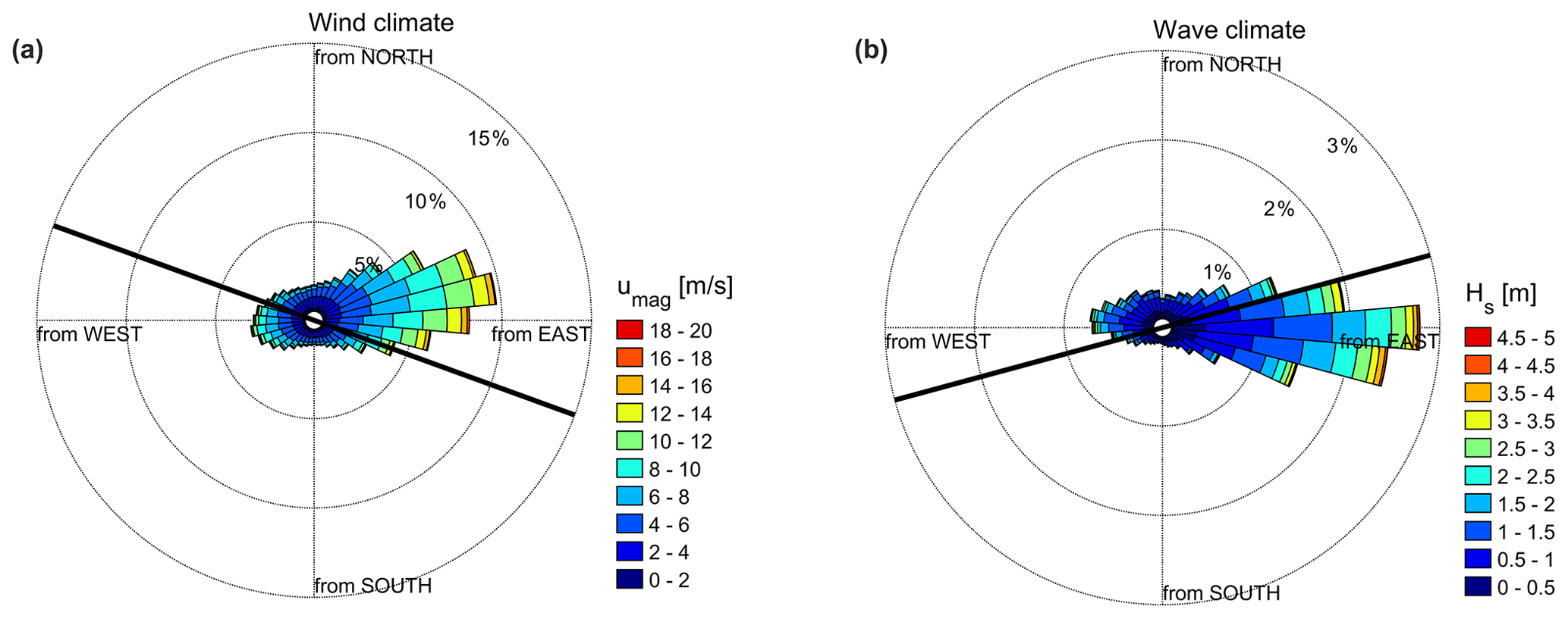
Figure 2Wind (left; a) and wave (right; b) climate at the single ERA5 output point of 72∘ N, 147∘ W for the time period 1979–2019 (see Fig. 1 for the location). In panel (a) the black line depicts the overall coastline orientation of 110∘ N, and in panel (b) it is the mean wave direction of 75∘ N.
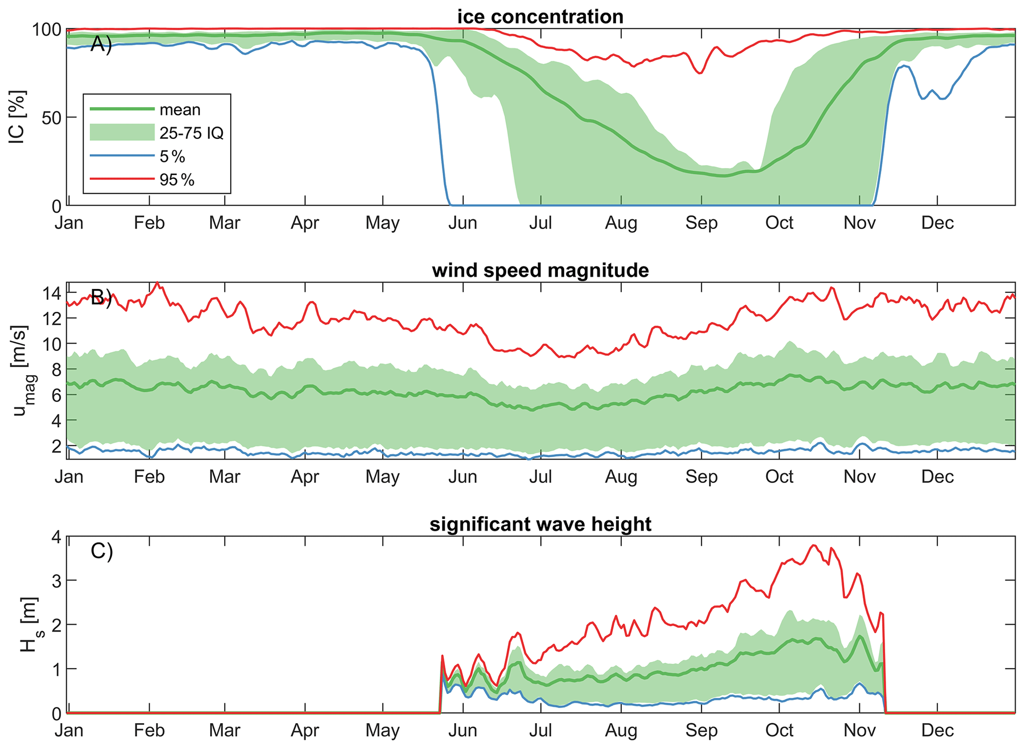
Figure 3Ice concentrations (a), wind speed magnitude (b), and significant wave height (c) at the single ERA5 output point of 72∘ N, 147∘ W (see Fig. 1 for the location) averaged daily over the time period 1979–2019. Each subplot shows the mean, 5 %, 25 %, 75 %, and 95 % exceedance probability. The interquartile range (IQ) is the area shaded green between the 25th and 75th percentiles.
3.1 Data sources
3.1.1 ERA5
ERA5 (Hersbach et al., 2020) is a detailed reanalysis of the global atmosphere, land surface, and ocean waves from 1950 onwards produced by the European Centre for Medium-Range Weather Forecasts (ECMWF). This meteorological dataset provides, among other variables, estimates of atmospheric parameters such as air temperature, pressure, wind, ice concentration, and information on waves over the global oceans. Atmospheric data are available at a resolution of 0.25∘ (∼30 km), while wave data can be retrieved at 0.5∘ resolution. The reanalysis combines model data with observations from across the world into a globally complete and consistent dataset using the laws of physics. ERA5 has been shown to perform well in capturing observed weather and climate variability in Alaska and the Arctic (Graham et al., 2019). It is however not able to resolve landfast ice (Hošeková et al., 2021). In particular, the authors show that the global reanalysis model has a good agreement with observed offshore wave heights. However, the persistence of landfast ice in the late spring/early summer is not well resolved, resulting in an overestimation of the cumulative spring coastal wave exposure. In this paper, offshore significant wave height (Hs), mean period (Tm), and mean direction (Dm) are used to drive the SWAN model. Wind conditions (u10, v10) and ice concentration (IC) from this reanalysis dataset are additionally applied across all model domains.
3.1.2 Field measurements
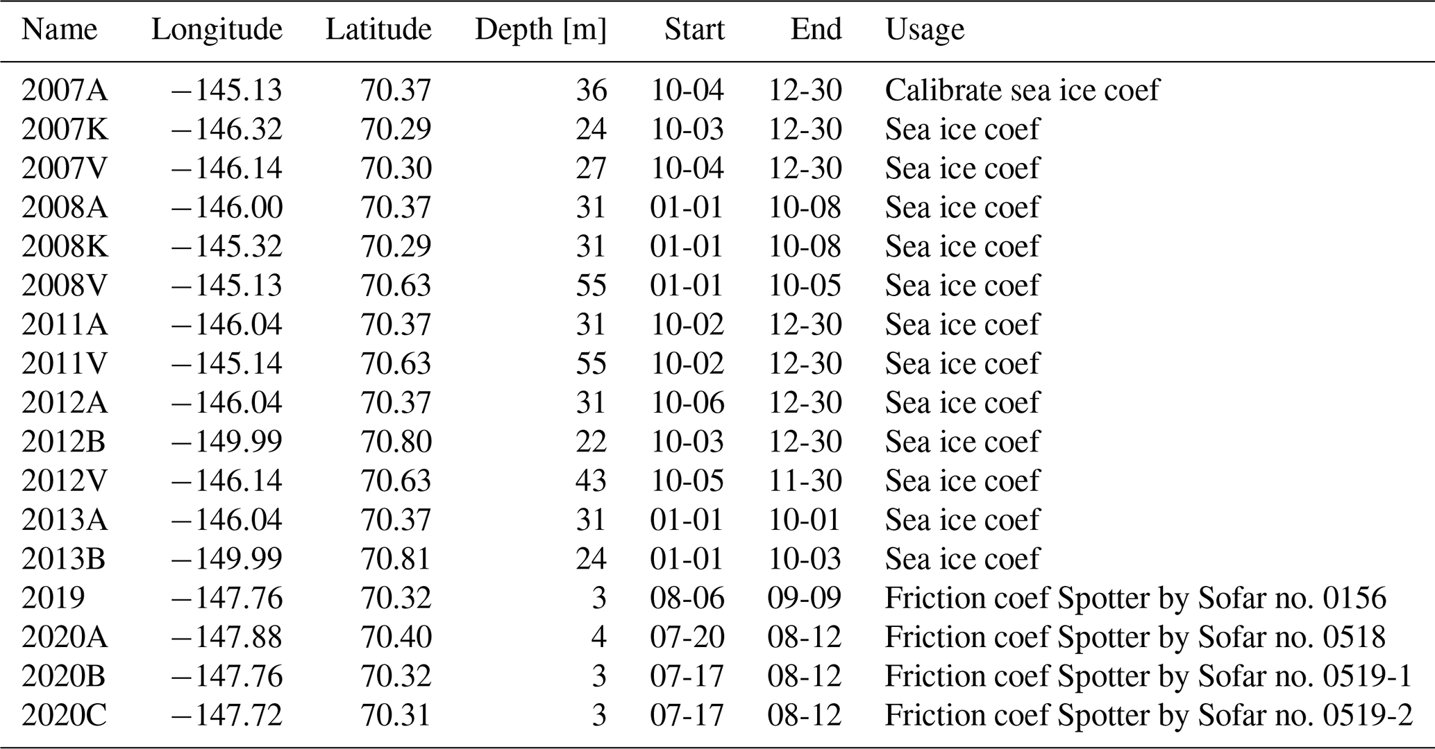
Limited in situ observational wave data exist within Beaufort Sea and particularly within FIB. As part of this study, existing wave observations from the 1980s until 2013 were gathered by combing several existing databases. High-quality observations collected by Shell Energy from 2007–2013 were selected to calibrate and validate the model. Data prior to 2007 provided daily wave height estimates measured with a “yardstick” and therefore deemed insufficiently accurate for this study. With the exception of one shallow-water (∼3 m) time series measurement in 1982 that was located outside the high-resolution model domain (Gallaway and Britch, 1983), all previously collected wave observations were in deep water (depth >20 m). Therefore, additional measurements were collected as part of the Bureau of Ocean Energy Management (BOEM) Central Beaufort Sea Wave and Hydrodynamic Modeling Study. Sofar Spotter wave buoys (Raghukumar et al., 2019) were deployed in shallow water for approximately 4 weeks each in the summer of 2019 and 2020. The buoys were set to broadcast standard bulk wave parameters (Hs, Tm, Dm, etc.) every hour via the Iridium satellite communication network. Three Spotter buoys were used in this study, deployed in 2019 (one time) and 2020 (two times). Spotter no. 0519 deployed in 2020 was dragged by ice and changed position and is therefore included twice in summary Table 1.
Table 1Overview of wave observations used for calibration and validation purposes in this paper. The name of each observation is a combination of the calendar year of deployment and a letter. Longitude and latitude are coordinates in degrees (WGS84). Depth is in meters relative to mean sea level. The start and end dates (mm-dd) of deployment are indicated. The comment provides more information including which measurement was used for calibration and validation for sea ice coefficients and friction coefficients and formulation.
3.2 Model
The spectral wind-wave model SWAN is widely used to compute wave fields over shelf seas, in coastal areas, and in shallow lakes. The accurate estimation of wave field statistics by such models is essential to various applications in these environments. SWAN computes the evolution of wave action density , where E is the wave variance density spectrum and σ is the relative radian frequency, using the action balance equation.
SWAN supports several bottom friction formulations (BFFs) that can be found in the literature. In this study, three formulations were tested: Hasselmann et al. (1973; Joint North Sea Wave Project, JONSWAP), Collins (1972; called Collins-BFF), and Madsen et al. (1988; called Madsen-BFF). Hasselmann et al. (1973) derived the simplest expression for bottom dissipation in which friction is a constant. From the results of the JONSWAP experiment, they found a value of 0.038 m2 s−3, which is also the default in SWAN. Madsen et al. (1988) derived a bottom friction formulation based on the eddy-viscosity concept in which the user specifies a bottom roughness length. The default bottom roughness length used by SWAN is 0.05 m. Collins (1972) derived a formulation for the bottom friction dissipation in which the turbulent bottom stress is related to the external flow. The user-definable variable is the drag coefficient which has a default value of 0.015 in SWAN.
Recently, Rogers (2019) implemented input–output for sea ice in SWAN, a dissipation source term, and scaling of wind input source functions by sea ice. This functionality is built on lessons learned during the implementation of sea ice in WAVEWATCH III (Collins and Rogers, 2017). The formulations use a simple empirical parametric model (polynomial function) for dissipation by sea ice, following Meylan et al. (2014) and Collins and Rogers (2017), which prescribe the dissipation rate as a function dependent on the wave frequency. Thus, the temporal exponential decay rate of energy can be written as
where Sice is the sea ice sink term and E is the wave energy spectrum. Here, ki has units of 1 m−1 and is the linear exponential attenuation rate of wave amplitude in space. Factor 2 provides a conversion from amplitude to energy decay. The group velocity, cg, enables conversion from spatial decay to temporal decay. Sice and E vary with frequency and direction. In the implementation of Rogers (2019), ki varies with frequency according to
with c0 to c6 being the user-defined empirical (calibration) polynomial coefficients. Rogers (2019) only used c2 and c4 and excluded the other coefficients (i.e., the remaining coefficients are zero). Throughout this study, we follow previous work and only calibrate using c2 and c4. The sea ice sink term is scaled with ice concentration. Sea ice thickness is not explicitly part of the equation but implicitly considered via the calibration coefficients.
Furthermore, the scaling of the wind input source functions allows the user to control the scaling of wind input by open-water fraction with the variable Ωiw (Rogers, 2019). The default value of Ωiw=0, used throughout this study, corresponds to the case where wind input is scaled by the total fraction of open water. For example, when 25 % of a grid cell is covered with ice, only 75 % of the original input source function of wind is applied in the simulation (1–0.25 = 0.75).
These formulations, also referred to as IC4M2, have been implemented in the main sub-version of SWAN since version 41.31, which is the version used in this study. Here, a three-level SWAN nested grid setup is used (Fig. 4) with grid resolutions of 5000, 1000, and 200 m for the overall, intermediate, and detail grids, respectively.
SWAN is run in third-generation mode and includes parameterizations for wind input, quadruplet interactions, triads, and whitecapping. SWAN is run with physics package ST6 (Rogers et al., 2012) that allows for a multiplier on the drag coefficient. Here we base the drag coefficient multiplier on the work of Le Roux (2009), which accounts for differences in air–water temperatures. SWAN normally does not include this effect, but the Le Roux formulation based on temperature difference is included here via the ST6 implementation. Based on the analytical wave height formulation of Le Roux, variations to the wave height because of variations in the drag coefficient multiplier are estimated to be between −10 % to +10 % (95 % confidence interval, CI) or a drag coefficient multiplier of ±20 %. Wave boundary conditions and meteorological forcing conditions are based on ERA5. In particular, u10 and v10 were used to generate wind waves. IC was used for the IC4M2 computation. Air temperature and sea temperature were used to estimate the drag coefficient of Le Roux. Numerical frequency resolution ranges lognormally from 0.03 Hz up to 2.5 Hz in 46 frequency bins (33.3–0.4 s); 5∘ bins are used to resolve wave direction.
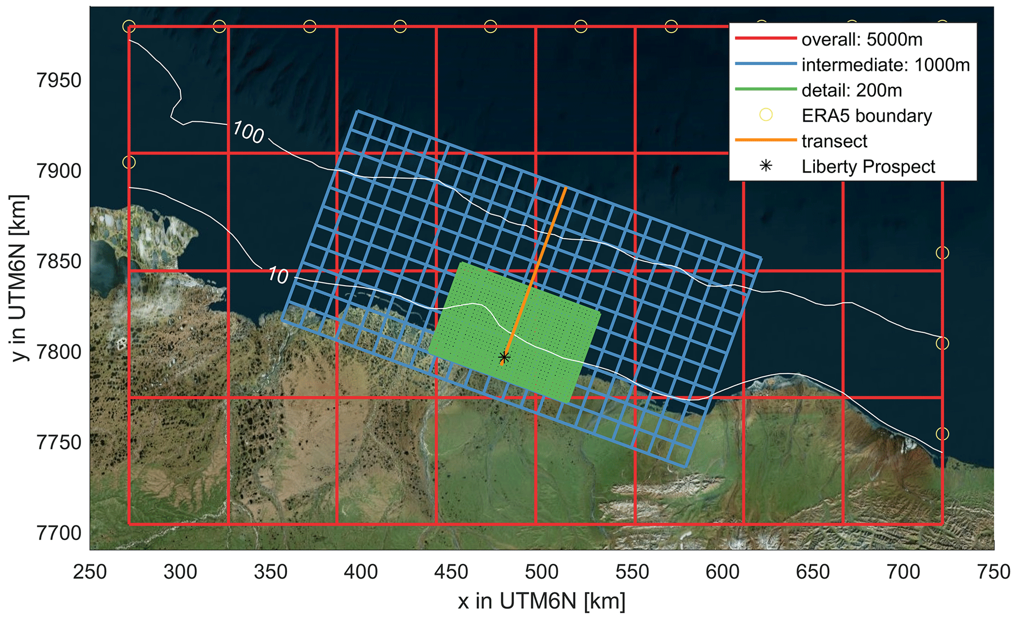
Figure 4Three-level SWAN model nests with the coarse overall (red), intermediate (blue), and fine detailed grid (green). The model resolution is 10 times denser than depicted in the figure. ERA5 wave boundary points are presented as circles. Black star denotes the location of the proposed construction of an artificial island in Foggy Island Bay. © Microsoft Bing Maps.
Calibration was performed via the testing of several friction formulations and coefficients. In particular, three bottom friction formulations (JONSWAP, Collins-BFF, and Madsen-BFF) were tested for the three coefficients each (i.e., 3×3 variations =9 times). Moreover, several empirical coefficients of the newly implemented ice formulations by Rogers (2019) were tested regarding the empirical (calibration) polynomial coefficients for dissipation and Ωiw.
3.3 Methods
Wave conditions across Beaufort Sea, Beaufort sound, and FIB were simulated with 3-hourly stationary SWAN simulations. First, the model was run over time periods with available field measurements to perform calibration and validation of the friction and empirical ice coefficients. Observations collected in 2007–2013 (offshore) and 2019–2020 (nearshore) were used to calibrate and validate the SWAN grid models (see next sections). Offshore measurements collected between 2007 and 2013 during partial ice cover were split into time periods for calibration and validation of the sea ice implementation. All model domains were utilized for the calibration and validation. In particular, 1439 time points during the partial ice season were selected for calibration purposes (∼20 % of the available timestamps with IC >5 %), and 11 430 time stamps in both the open-water and ice season were used for validation. Spotter data collected from within the shallow region of FIB during the 2019 open-water (i.e., ice-free) season were used to calibrate the friction formulations and coefficients. In addition, 2020 nearshore Spotter data were used to validate the finest-resolution grid and nearshore wave heights. Second, the calibrated SWAN model was used to hindcast wave conditions from 1979 to 2019. Both the open-water (IC <5 %) and ice (IC >5 %) season were simulated. Years were simulated individually, and once completed, they were combined into one 41-year time series per grid cell with a temporal resolution of 3 h.
3.3.1 Wave parameters
Throughout this paper, the following wave parameters were used. In particular, the significant wave height (Hs; Eq. 3 in meters), mean wave period (Tm or Tm0,1; Eq. 4 in seconds), steepness (s; Eq. 5; dimensionless), mean wave direction (Dm; Kuik et al., 1988; in degrees relative to north), and wave power (P; Eq. 6 in J m−1 s−1) were used. We acknowledge that other wave period could be used that give more weight to either lower frequencies () or higher frequencies (Tm0,2). Sofar Spotter wave buoys directly reported Tm01, while 2007–2013 data from Shell were converted from peak wave period to Tm01 with a transformation constant of 1.2 (Goda, 2010):
in which m0 is the zero moment of the spectrum and m1 is first moment of the spectrum. L is wavelength; ρ is the density of water; and g is the gravitational constant.
3.3.2 Skill scores
To assess model skill, several metrics were used. In particular, the model bias, mean absolute error (MAE; Eq. 7), root mean square error (RMSE; Eq. 8), and scatter index (SCI; Eq. 9) were computed. The latter gives a relative measure of the RMSE compared to the observed variability.
in which yi is the computed value, xiis the observed value, and N is the total number of data points.
3.3.3 Trend analysis
Summary statistics of Hs, Tm, Dm, P, s, IC, and wind speed (umag) were computed. The median, 90th percentile (or 10 % exceedance probability), and maximum values for each variable were computed for several daily, monthly, seasonal, and yearly periods. Additionally, the annual count of rough wave days (τro), defined as the number of days when Hs exceeds 2.5 m yr−1 (WCRP, 2020), were computed. Also, the number of open (IC <5 % ice) and closed days (IC >85 %) were determined for the area of interest.
The non-parametric Mann–Kendall (MK; Mann, 1945; Kendall, 1975) test was then applied to detect monotonic trends, and the magnitude of the trends was calculated with Sen's slope (Sen, 1968). The MK test is a test to statistically assess if there is a monotonic upward or downward trend of the variable of interest over time. The MK test is non-parametric (distribution-free) and does not require that the residuals of the fitted regression line be normally distributed. However, the standard p values derived from the MK test assume that the observations are independent realizations. Following the method used by Wang and Swail (2001), the effects of autocorrelations are accounted for in assessing trends and their significance. A pre-whitened time series (i.e., processed to make it behave statistically like white noise) that possesses the same trend as the original signal is computed and re-computed via an iterative approach to find the best fit line (Sen's slope) and adjusted p value (Reguero, 2019).
The wave calibration is divided into simulations for observation periods during the open-water season and ice season. This division is made by partitioning the observations based on the mean IC in the area of interest. When the mean IC was higher than 5 %, it was deemed part of the ice season. When the mean IC was smaller than 5 %, it was deemed part of the open-water season. In particular, 2019 observations were used for open-water season calibration, and ∼20 % of the available timestamps in the data from 2007–2013 were used for the ice season calibration.
4.1 Open-water season
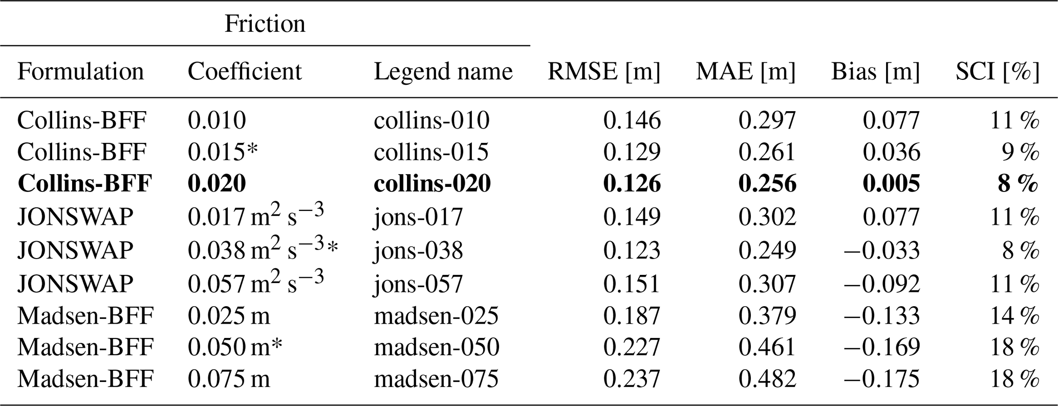
Observed and computed wave heights and periods for the 2019 measurement period are shown in Fig. 5. Individual combinations of bottom friction formulation and friction coefficient are plotted with different colors. Observed wave heights and periods are plotted as black dots. The figure shows strong sensitivity to different friction options used for both the wave height and period. The range of coefficients used for the Madsen et al. (1988) formulation (Madsen-BFF) resulted in too much dissipation due to bottom friction and underestimated wave heights. Whereas default SWAN values for Collins-BFF and JONSWAP (see Table 2) performed well, the overall best fit, based on visual inspection of the time series in Fig. 5 and residual plots (not shown) as well as quantitative error statistics, was the formulation of Collins-BFF with a coefficient of 0.020 (RMSE = 0.126 m; bias = 0.005 m).
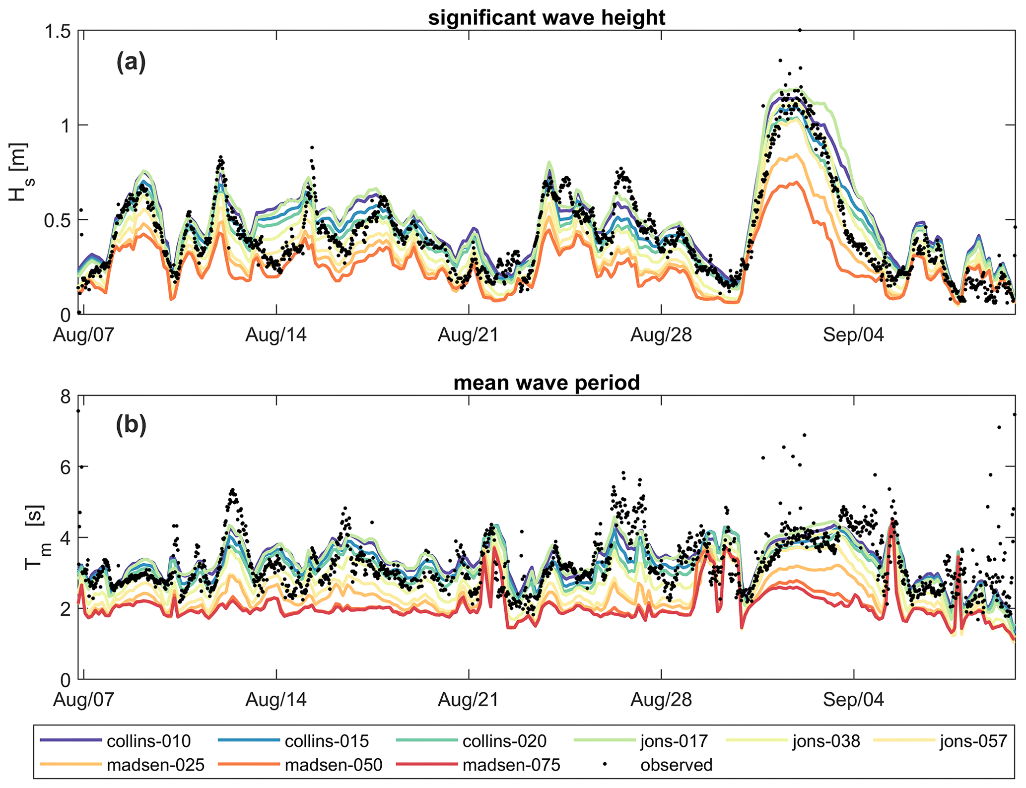
Figure 5Wave height (a) and wave period (b) as observed (black dots) and modeled (colored lines) with the detailed domain using various friction formulations and coefficients for the observation period in 2019. Measurements were obtained with a Sofar Spotter anchored at 70.32∘ N, 147.76∘ W in approximately 3 m water depth. Please note that the date format in this and following figures is month/day.
Table 2Skill scores for computed significant wave heights (Hs) using various bottom friction formulations (BFFs) and coefficients. The Collins bottom friction formulation (Collins-BFF; Collins, 1972), with a coefficient of 0.020, was chosen for the remainder of this study (denoted in bold). Friction coefficients with an asterisk (*) are SWAN “default” values. The JONSWAP friction formulations are from Hasselmann et al. (1973), and the Madsen friction formulations are from Madsen et al. (1988).
4.2 Ice season
Observed and computed wave heights and periods for the 2007 measurement campaign are shown in Fig. 6. All individual combinations of empirical ice formulations are plotted with a different color (see Table 3 for a description per combination). Observed wave heights and periods are plotted as black dots. The results show a strong sensitivity to these empirical coefficients. Moreover, the SWAN models miss certain events that ERA5 can reproduce likely due to the assimilation of altimeter measurements. For example, the event at the end of November 2007, when wave heights around 5–6 m were observed, was captured in ERA5 but strongly underestimated by SWAN. The observations also have gaps when no waves were observed.
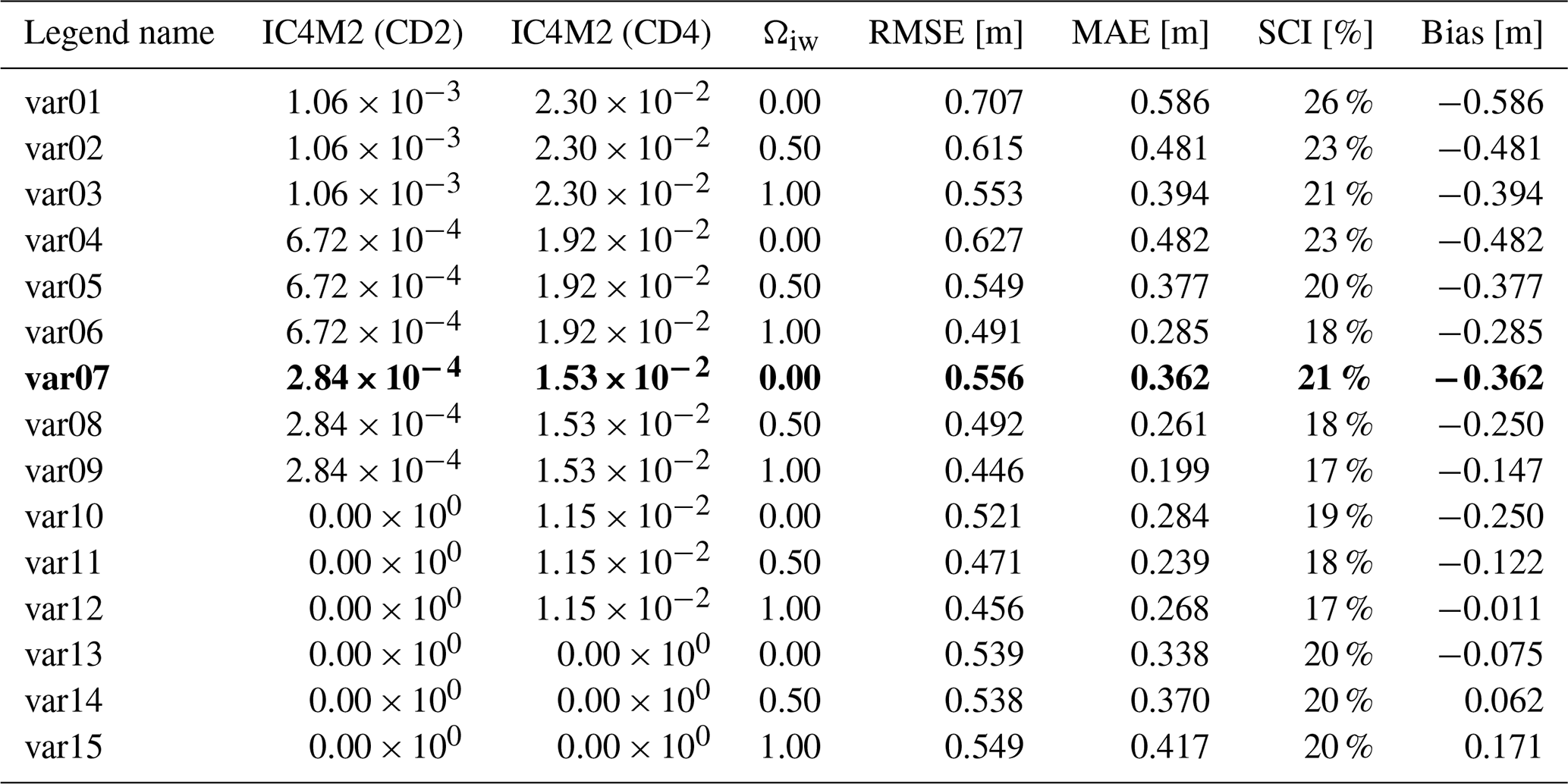
Table 3 summarizes model skills for wave height and period for 20 % of the offshore data between 2007–2013 combined (1439 time points). Based on these results, the lower IC4M2 coefficient is most appropriate. Values of and , for c2 and c4, respectively, in the equation, as Meylan et al. (2014) found for ice floes in the MIZ near Antarctica, resulted in a strong negative bias (i.e., model underestimates; too much dissipation). On the other hand, values of and , as found by Rogers (2019) for pancake and frazil ice, resulted in a better agreement with observations.
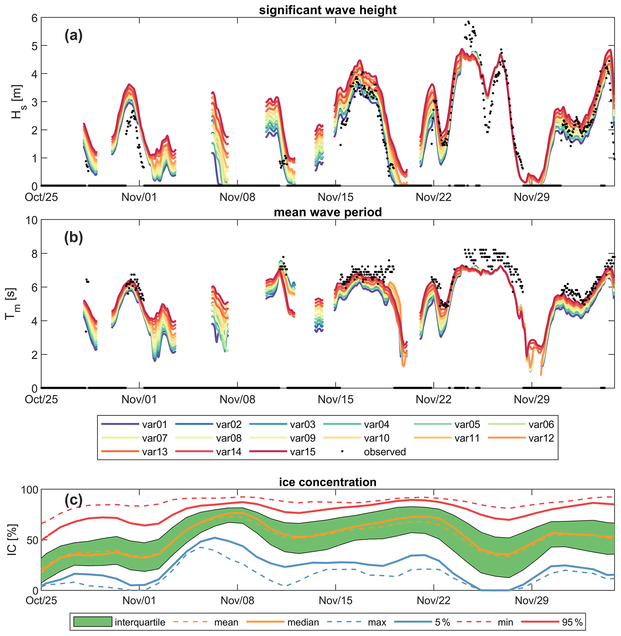
Figure 6Wave height (a) and wave period (b) as observed (black dots) and modeled (colored lines) with the detailed intermediate domain using various combinations of empirical ice formulations (Table 3) for the observation period in 2007. Ice concentrations (IC; panel c) are high across the domain. The different colors in panel (c) show the mean, 5 %, 25 %, 75 %, and 95 % exceedance probability. The interquartile range (IQ) is the area shaded green between the 25th and 75th percentiles.
Table 3Significant wave height model skill for different combinations of empirical ice coefficients describing dissipation and reduction in wave growth; var07 (bold) is the chosen value for the remainder of this study. All 1439 observations with at least a mean ice concentration of 5 % from 2007–2013 are considered.
5.1 Nearshore validation
Observed and computed wave heights and periods for the 2020 measurement campaign are shown in Fig. 7. Similar to previous figures, model results are plotted with colored lines, and observed data are black dots. The figure shows that generally increasing model resolution improves reproductive skill. In particular, the detail model domain has the lowest RMSE of 0.133 and 0.118 m for 2020A and 2020B+C, respectively. However, the overall and intermediate model domains also have good model skill for the nearshore Spotter observations. The detailed domain results in a ∼20 % reduction in RMSE but with an ∼80 % increase in computation time. Model resolution cannot explain the mismatch for the time periods of 27 July–1 August and ca. 6 August, where larger differences between observations and measurements can be seen.
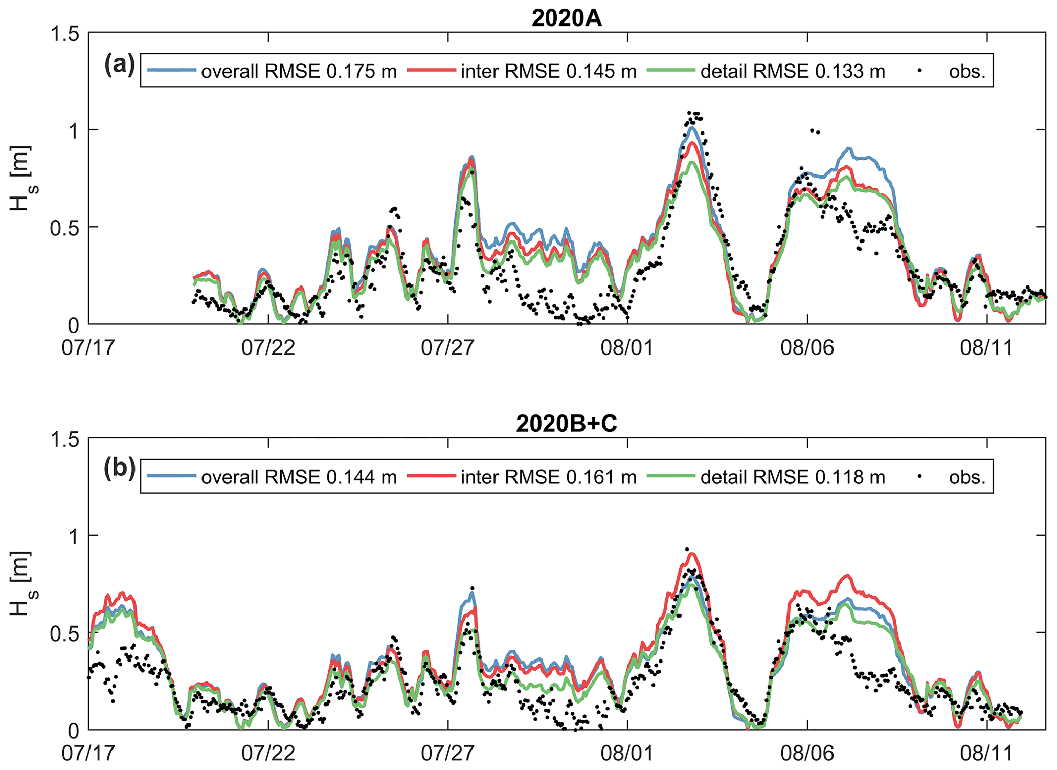
Figure 7Significant wave height as observed (black dots) and modeled (colored lines). Three model domains are presented: overall (red), intermediate (blue), and detailed (green) domain. Upper panel (a) is 2020A (Spotter no. 0518), and bottom panel (b) is 2020B and 2020C (Spotter nos. 0519-1 and 0519-2). See Fig. 1 for the extent and locations of these grids.
5.2 Large-scale validation
The calibration coefficients found in the previous section for the open-water (i.e., friction formulation and coefficient; Collins-BFF of 0.020) and ice season (i.e., empirical coefficients for ice dissipation and reduction on wave growth; var07) are validated for the remaining observation time points not used within the calibration period. In particular, 11 430 time stamps (80 % of the offshore data between 2007–2013) in both the open-water and ice season were used for large-scale validation. This approach allows for independent validation of the model. Figure 8 presents scatter density plots for the modeled and observed significant wave height (Fig. 8a) and mean wave period (Fig. 8b) as modeled with the intermediate grid. The model slightly overestimates both the wave height (bias of 19 cm) and period (1.3 s). SCIs for wave heights and periods are around 30 %. This is deemed acceptable to assess changes in the wave climate.
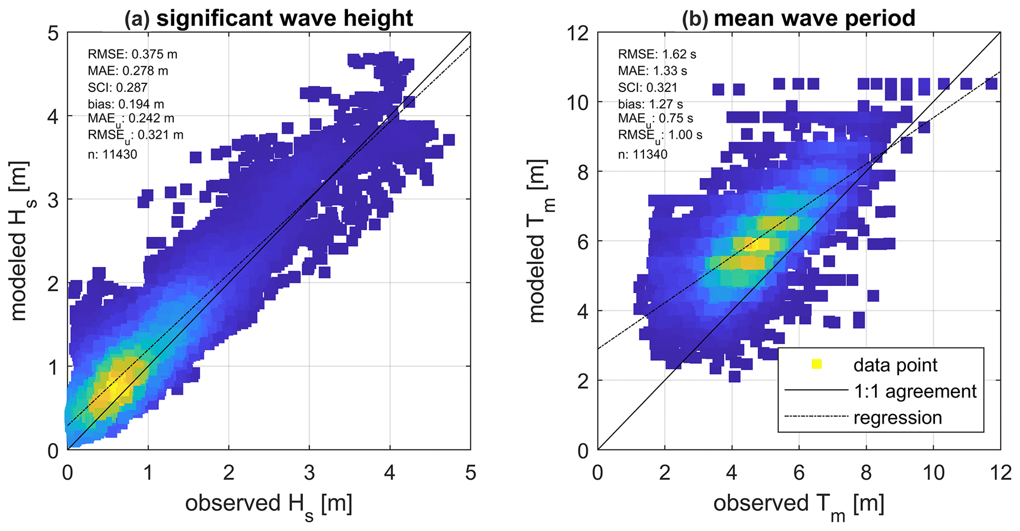
Figure 8Scatter density plots of the modeled and observed wave parameters for >10 000 timestamps for the combined dataset of observations collected between 2007–2013 for the intermediate domain. (a) Significant wave height and (b) mean wave period.
In this section, a 41-year hindcast of waves simulated with SWAN is analyzed. First, changes in meteorological conditions, including changes in ice concentration and the number of open-water days and historical winds, are presented (Figs. 9 and 10). Second, changes in wave height, period, wave power, and direction are visualized and quantified. Table 4 presents an overview of the results per month, season, and year. Figure 11 presents an overview of the main changes in climate for September, October, and November (SON).
6.1 Changes in meteorological climate
6.1.1 Wind
Wind speeds and direction vary from month to month, with higher extremes between about October and May. Figure 9 presents the number of days during which the study area had a Beaufort scale value of <4 (gentle breeze), 4 (moderate breeze), 5 (fresh breeze), 6 (strong breeze), and >6 (gale force) based on the wind speed magnitude in ERA5. Although there is year-to-year variability, visually, no trends emerge. Spatial variability (not shown) reveals that median wind speeds are fairly constant along the coast but decrease in the cross-shore direction from sea to land. In contrast, annual extreme wind speeds are higher in the southeastern corner of the domain with an annual wind speed close to 21 m s−1. The MK test of the annual extreme winds reveals a statistically insignificant median trend of +0.01 m s−1 yr−1 (or less than +0.1 % yr−1).
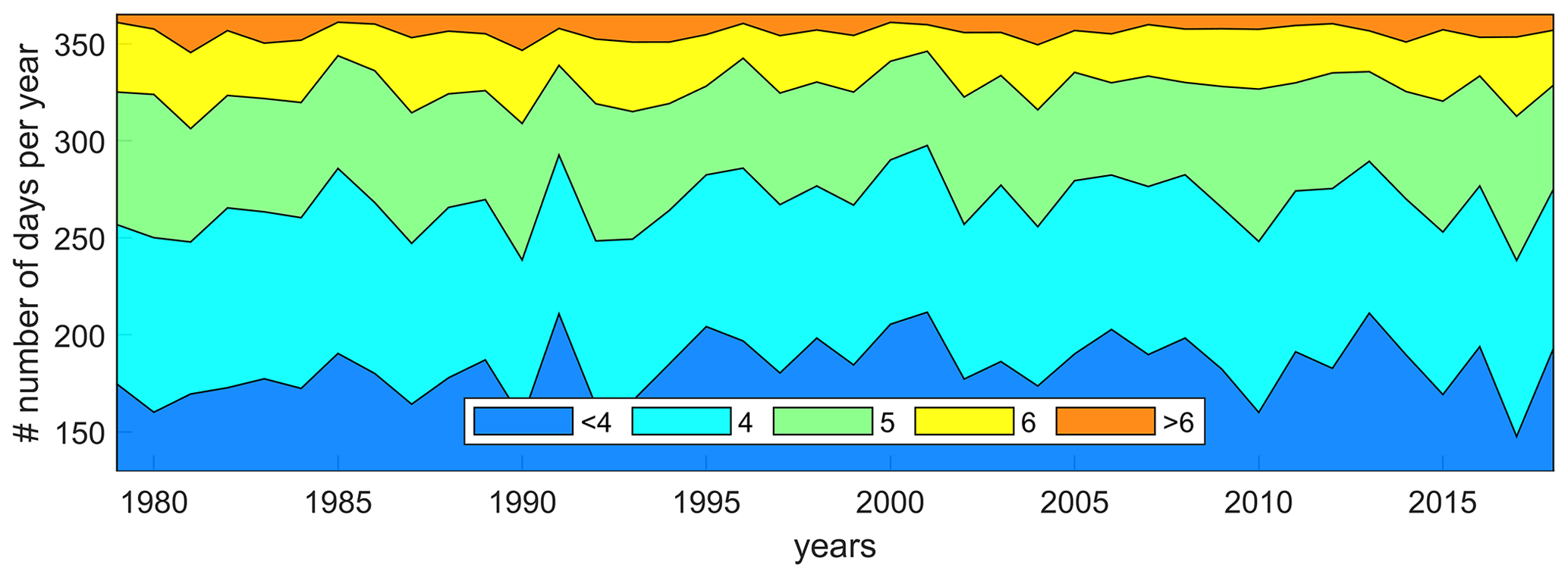
Figure 9The number of days with the Beaufort scale: <4 (gentle breeze), 4 (moderate breeze), 5 (fresh breeze), 6 (strong breeze), and >6 (gale force) as simulated by ERA5 for the area of interest. Data are based on the average wind speed for the intermediate domain.
6.1.2 Sea ice
Ice concentration varies considerably from month to month. As shown in Fig. 3a, the maximum duration of the open-water season is from June–November with the lowest concentration around September–October. Figure 10 presents the number of days per year during which central Beaufort Sea (see Fig. 1 for location) was fully closed (IC >85 %), open (IC <5 %), or in an intermediate state. The trend lines reveal a large decrease in the number of days the area of interest was covered with ice and a similar increase in the number of days it was fully ice-free. For example, in 1979, on average, the area was closed for ∼250 d and only fully open for a few weeks. In 2019, 41 years later, this has changed to 195 and 110 d, respectively. This equates to an 8-fold increase in the number of open-water days. This increase in open-water days is driven both by earlier sea ice breakup and later freeze-up.
Moreover, the MK test reveals a statistically significant trend of decreasing median IC of −1.3 % yr−1 and −1.7 % yr−1 for the summer (June, July, and August; JJA) and fall (September, October, and November; SON), respectively. Figure 11a presents the 41-year median IC for SON and the trend of IC for SON (Fig. 11b) for the area of interest. Spatial variability reveals median ice concentrations (IC50) to be the lowest (close to zero) in the northwest of the area of interest and highest in the southeast (around 25 %). A larger negative gradient occurs closer to the shoreline (around the 10 m depth contour) and in the areas with generally higher concentrations. IC50 trends have a statistically significant trend across the area of interest. Table 4 shows similar patterns as seen visually. Statistically significant decreasing trends in ice concentration occur in the months of July–November, with October being the month with the most significant negative trend.
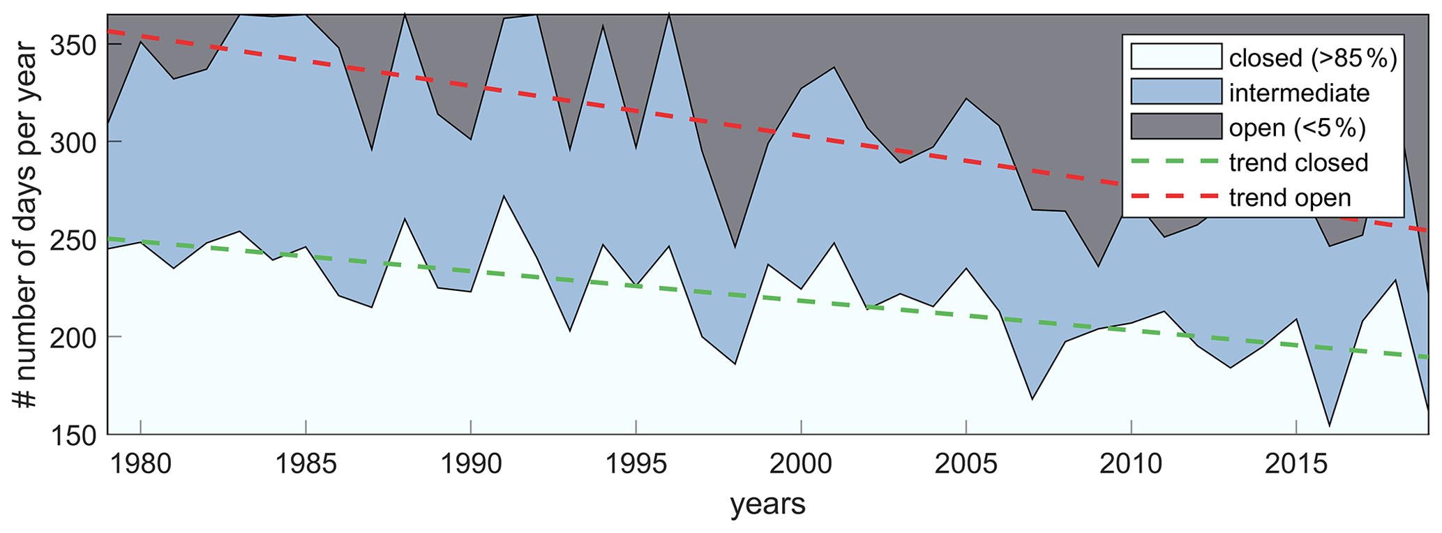
Figure 10The number of closed (IC >85 %), intermediate, and open (IC <5 %) days based on the percentage ice cover as simulated by ERA5 for the central Beaufort Sea. Trend lines for the number of closed days (green) and open days (red) are presented as dashed lines. Data are based on the single ERA5 output point of 72∘ N, 147∘ W for the time period 1979–2019 (see Fig. 1 for the location).
6.2 Changes in wave climate
6.2.1 Wave heights
Wave heights vary widely from month to month because of the seasonality of IC. As shown in Fig. 3, waves occur mostly from late May to November, depending on the ice concentration. Figure 12a presents the daily median wave height (Hs50) for 41 years based on simulated conditions averaged across FIB. In general, no waves are present during the months of December to June, when ice concentration is near 100 %. Strong year-to-year variations are evident, but visually it is clear that wave heights have increased substantially in the last 40 years. In 1979, Hs50 values higher than 0.5 m were present only from ca. August–October. In 2019, this period extended to ca. July–November. This pattern correlates strongly with changes in IC in the area (correlation coefficient r of −0.70 for daily Hs50 and IC50).
These visually observed trends are quantified by the MK test of the 10 % exceedance wave height (Hs90). Spatial variability in Hs90 and trends for the fall season (SON) are presented in Fig. 11c and d. Wave heights are higher in the northwest (Fig. 11c). This is a similar pattern as seen in IC shown in Fig. 11a. Moreover, a clear trend of increasing Hs90 can be seen in Fig. 11d. There is hardly any alongshore variability in the increasing trend. This might be because of the somewhat coarse ERA5 wave and wind resolutions. However, there is a cross-shore variability with larger increases in Hs90 offshore than closer to the shoreline. The increase in Hs90 is estimated to be around % yr−1 (or 3.92±1.06 cm yr−1)1. Table 4 presents the median in Sen's trend values for the Hs90 for all months, seasons, and annually. These larger (Hs90) waves mainly occur in September and October, with a median value of around 2.0 and 2.4 m, respectively, for September and October based on the 41-year-long hindcast. For October, Hs90 is increasing by 6.5±1.7 cm yr−1 (or % yr−1). This pattern correlates with the largest decrease in IC. In particular, a negative correlation of 0.87±0.02 is found for the entire dataset for monthly Hs90 and IC50.
Similar trends are found for the more extreme wave conditions. In particular, the annual maximum wave height (Hs,max) and the number of rough days (τro) were computed from the 41-year dataset. Figure 13a presents the Hs,max across FIB as a function of time. The spatial median annual Hs,max is depicted as black dots, and the spatial variability in the annual Hs,max is depicted as uncertainty bars. Strong year-to-year variability is visible; however, a statistically significant increasing trend of around 4.1 cm yr−1 (or +1.1 % yr−1) was found, resulting in an increase in a spatially median Hs,max from 2.90 m in 1979 to 4.62 m in 2019. Similar to the Hs90 during SON (Fig. 11c), annual Hs,max values show cross-shore variations but little to no alongshore variation. Closer to the shoreline, processes such as whitecapping and breaking dissipate wave energy occur. This depth-induced saturation aligns very closely with the 10 m depth contour. Within the shallow FIB, wave height tends to have a maximum of ∼1.9 m, implying a depth-induced saturation that corresponds to a height–water depth ratio (γ) of 0.4 (depth is ∼5 m). The rather low γ value is typical of field studies (Raubenheimer et al., 1996) and smaller than γ of ∼0.6–0.78 found for more simplified cases. Raubenheimer et al. (1996) report γ as low as ∼0.3 for field studies and attribute such low values to bottom friction and whitecapping by strong winds through wave energy dissipation near the shore.
Moreover, the largest wave events seem to be happening later and later in the calendar year. An analysis identified per calendar year the annual maximum wave height of the year and associated storm date. The result is a list of 41 annual maximum wave heights and associated storm dates per calendar year. In 1979, the average storm date occurred on 24 September (day 269); in 2019 this has increased to 15 October (day 289). This shifts the average storm date 20 d later in the calendar year and results in storms with generally higher wind speeds on top of the general decreasing IC (Fig. 13b).
Increasing occurrences of high wave events, τro, are also identified. Within the simulated 41 years, a statistically significant trend of 0.24±0.10 d yr−1 (or % yr−1) was determined. This equates to an increase from 1.5 to 13.1 d each year with high wave events in the offshore region. These rough days mainly occur during the fall months of September and October (see also Table 3).
6.2.2 Wave periods and steepness
Figure 11e and f present the median Tm and computed Sen's trend for the fall months. The median wave period varies slightly from offshore to nearshore, with offshore values reaching as high as 4.7 s and nearshore values being as low as 3.1 s. The wave period tends to increase over the analyzed period, and the trend is statistically significant. The increase in Tm varies spatially, with little increase in the shallow areas of FIB up to an increase of 0.03 s yr−1 in the deeper offshore parts of Beaufort Sea. This increase in period is relatively small compared to the median value (i.e., increase of % yr−1). The increase in wave period is most likely related to the increase in fetch length of the larger domain, which allows for more wave development. On the other hand, the median wave steepness of 0.0536 varies slightly in the cross-shore direction (not shown). Sen's trends of the wave steepness are all statistically insignificant and minor (−0.15 % to +0.23 % yr−1 for 97.5 % and 2.5 % exceedance). Therefore, based on the model results, the wave period increases proportionally with the wave height while maintaining similar wave steepness.

Figure 11Overview plot of the median value over 41 years of intermediate simulation for ice concentration (IC50; panel a), 10 % exceedance probability wave height (Hs90; panel c), median wave period (Tm50; panel e), and median wave direction (Dm50; panel g). Sen's trend (panels b, d, f, h) for the same parameters in the fall season (SON). Statistically significant trends are stippled. Contour lines are the 100 and 10 m water depths. The black star is the proposed location for the construction of an artificial island in FIB. © Microsoft Bing Maps.

Figure 12Time series of the daily median significant wave height (Hs50) for 41 years of wave data across Foggy Island Bay as simulated by the intermediate SWAN domain (a) and daily median ice concentration (b). Time series are smoothed by applying a moving weekly filter. The median estimate for 1979 and 2019 is based on a linear fit per day of the individual years.
6.2.3 Wave direction
Figure 11g and h present the annual median Dm and computed Sen's trend. Offshore waves have a mean incident wave direction of 70–75∘ (nautical convention, clockwise from geographic north; i.e., traveling from northeast towards the southwest) near the 100 m isobath. This is (unsurprisingly) identical to the ERA5 wave rose of Fig. 2. Hence, incident wave directions in the offshore region strongly reflect the boundary conditions. In shallower waters approaching the shore, the waves refract towards the coastline, resulting in a mean wave direction of 48–54∘ (25th–75th percentile) around the 10 m isobath. Computed Sen's trends show counterclockwise rotation up to 0.39∘ yr−1. These trends are larger closer to the shore in shallower water and statistically significant. Closer to the offshore boundary, the trends are closer to 0∘ yr−1 but are statistically insignificant. Table 4 presents the breakdown of the median wave direction over all the different months and time periods. The median wave direction hardly changes for any of the analyzed months. However, for the seasons and yearly median wave direction, there is a statistically significant negative trend.
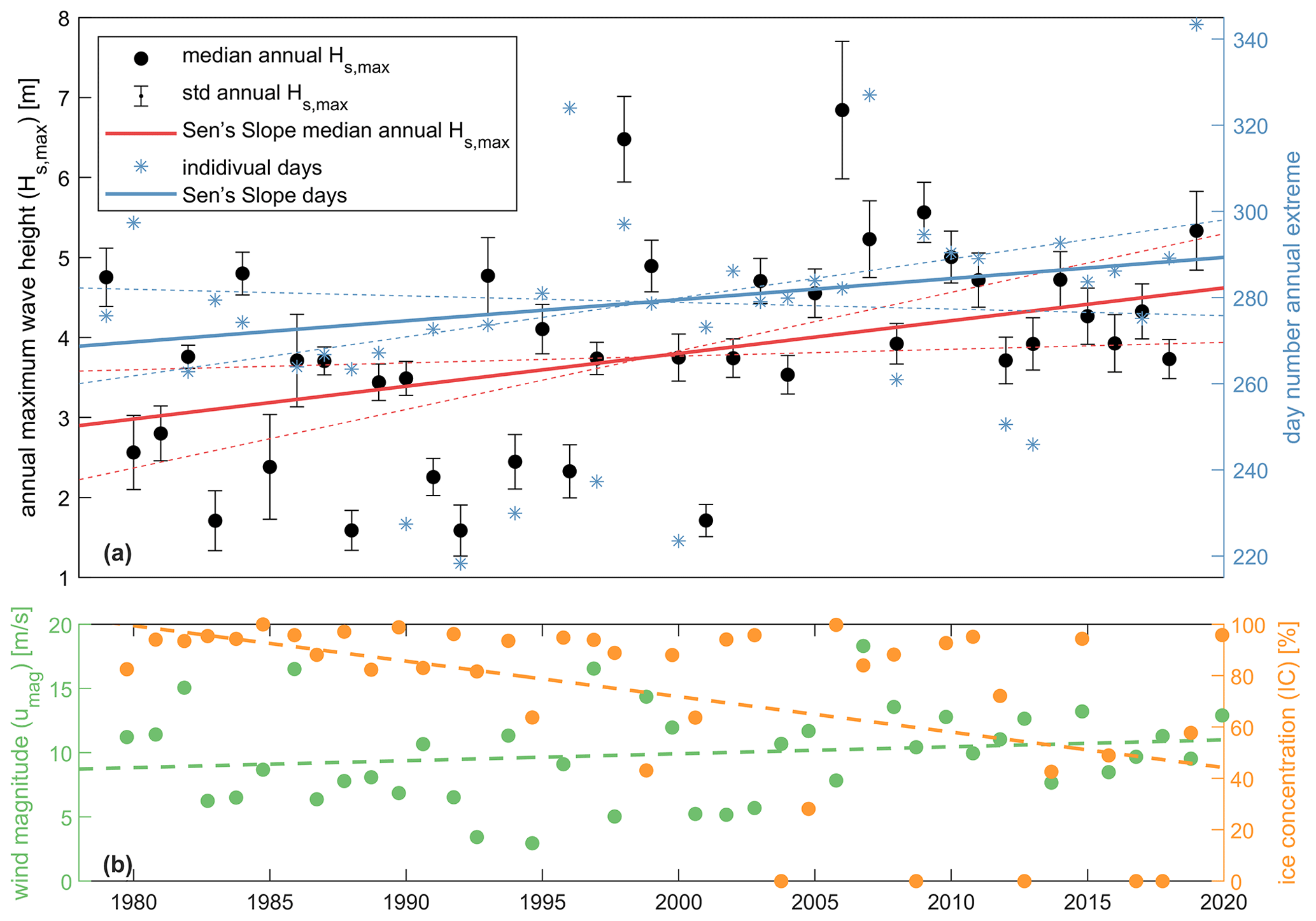
Figure 13(a) Time series of the annual maximum wave height (Hs,max) over the last 40 years as simulated with SWAN for the intermediate domain with an estimate of day number of the associated peak. The range represents 1 standard deviation (SD) based on spatial variability within the domain. The solid line is Sen's slope including the dashed uncertainty range for an alpha of 0.05 (dashed lines). (b) Ice concentration and wind speed during the storm based on ERA5 (circles) including linear fit (dashed lines).

Figure 14Median over 41 years of monthly cumulative wave power (P) along a transect (see Fig. 4) from nearshore (left) to offshore (right). Different colors represent different months and are cumulative (a). Associated bathymetry and water depth (MSL: mean sea level) (b). The green line in the lower panel marks the location of the Liberty Prospect project.
6.2.4 Wave power
Figure 14 presents the cumulative yearly wave power per month averaged over all the years simulated. Wave power is highest offshore in deep water and reduces closer to the shoreline. At the 10 m depth contour, the average cumulative yearly wave power is ∼70 % of the offshore wave power. At the 2 m depth contour, this decreases to ∼25 %. Preliminary analysis suggests that refraction on the shelf, dissipation (whitecapping and bottom friction), and blocking of wave energy due to the barrier islands all play a role. Figure 15 presents the cumulative wave power at Liberty Prospect in FIB; 5-year smoothed values for cumulative power and mean ice concentration in the shallow FIB have a strong inverse correlation of −0.986. The yearly cumulative wave power increased 5-fold over the 41 years analyzed. Also, the computed trend reveals a statistically significant increase in the wave power which is in absolute terms the largest offshore and less in the shallow parts of FIB. However, in relative terms, the increase in wave power is almost constant across the domain. In particular, a statistically significant value of Sen's trend of 3.9±0.2 % yr−1 is computed for the offshore compared to 3.8±0.2 % yr−1 at the 10 m depth contour. Table 4 presents the breakdown of the mean wave power over all the different months and time periods. Average wave power is small and hardly changes for the months of December–June. For the months of July–November there is a statistically significant increasing trend in wave power with the maximum increase occurring in October. Similar trends emerge with the dominant months of July, August, September, October, and November, explaining 93 % of the wave power together, and this importance hardly varies in the cross-shore direction or with time.
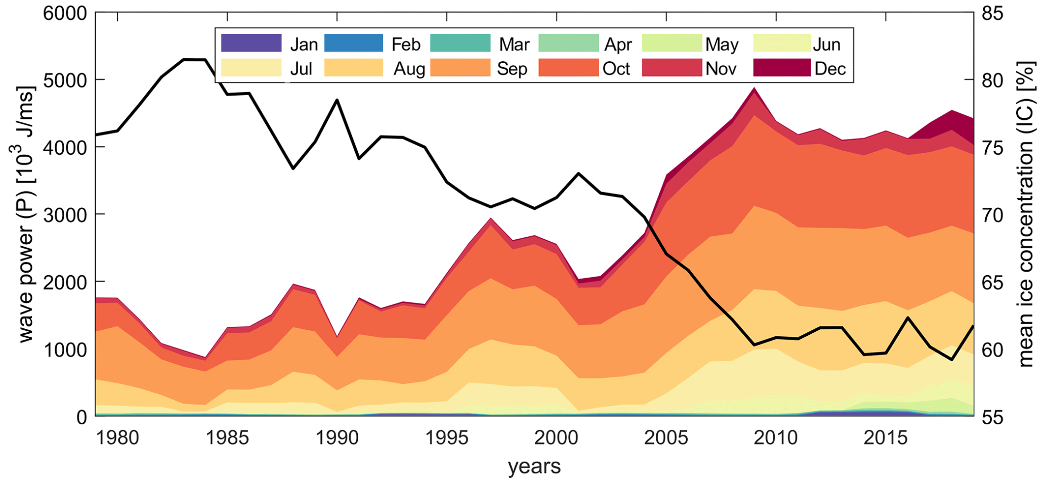
Figure 15Yearly cumulative wave power (P) smoothed over 5-year moving windows at Liberty Prospect in Foggy Island Bay. Different colors represent different months. The black line is the yearly mean 5-year smoothed ice concentration.
Table 4Trend analysis of the median ice concentration (IC50), 90th percentile wave height (Hs,90), median wave period (Tm,50), mean wave power (P), median wave direction (Dm,50), and the number of rough days (τro) based on values of the intermediate domain. Median and mean values computed over the entire 40 years of simulated data. Computed Sen's trends where the majority of grid cells show a statistically significant trend (assuming alpha of 0.05) are depicted in bold; otherwise, the trend is shown in the normal black color. DJF: December, January, and February. MAM: March, April, and May. JJA: June, July, and August. SON: September, October, and November.

The validation presented here shows that the constructed SWAN model can reproduce waves during the open-water and MIZ seasons. This reproductive skill has been achieved by forcing the model with ERA5 meteorology and with the inclusion of air–sea temperature differences (Le Roux, 2009) and new formulations by Rogers (2019) that account for the effect of ice on (reduced) wave growth and dissipation. An efficient and accurate model-based approach allowed for continuous 41-year simulations of waves across Alaska's central Beaufort Sea coast and the detailed quantification of changes in the wave climate across the seasons in shallower water than previous studies analyzed.
In the current literature, there is a consensus that larger ice-free areas, which persist longer into the fall, force higher sea states across Beaufort Sea (e.g., Thomson et al., 2016; Liu et al., 2016; Stopa et al., 2016). To our knowledge, no previous study has rigorously quantified how wave patterns vary within the near- and inshore regions of the central Alaska Beaufort Sea and across different seasons over the 41-year simulation period. Within the Beaufort–Chukchi Sea domain, Thomson et al. (2016) found that altimeter-derived measurements of wave energy increased between 2007 and 2014 and that modeled wave heights increased by 1 cm yr−1. Stopa et al. (2016) estimated an increase in wave heights up to 1 % yr−1 between 1992 and 2014. Findings of listed authors contrast with this study which suggests larger increases in wave heights over time. In particular, Hs50 increased by 6 %, and Hs90 and Hs,max increased up to 3 % and 1 %, respectively, over the 41-year hindcast period. We hypothesize that trends are strongly influenced by specifics of the analysis method, different wind and ice boundary conditions, locations and spatial extents, and the timeframe considered, and therefore different studies should be compared qualitatively instead of quantitatively.
Nearshore wave hindcasting is sensitive to wind forcing, dissipative/restrictive effects by ice, and boundary conditions from larger-scale models. Similar to several previous studies (e.g., Overeem et al., 2011; Barnhart et al., 2014; Stopa et al., 2016; Erikson et al., 2020), this study found that sea ice minimum now occurs later in fall, when the wind speeds also increase, which creates more favorable conditions for wave development. However, wind speed magnitudes and thus wave heights might be underestimated due to known biases in extreme wind speeds. For example, Liu et al. (2016) found underestimations of ERA-Interim for the Arctic Ocean. Moreover, validation of ERA5 wind speeds at Prudhoe Bay shows an underestimation during storm conditions (see Supplement). In contrast, wave energy may be overestimated during breakup and freeze-up due to poorly resolved ice concentrations within the nearshore (e.g., ERA5 ice concentrations used in this study are on a scale of ∼50 km, compared to the intermediate model domain of ∼250 km × ∼100 km). For example, Hošeková et al. (2021) found that while ERA5 reproduces the annual ice cycle well, this reanalysis product does not resolve landfast ice. The relatively coarse resolution of ERA5 in general is a limitation of this study, since small-scale wind variations and air–sea temperature gradient in the MIZ are not resolved. Model skills for the ice season (IC >5 %) could only be assessed with offshore field measurements. The nearshore validations showed good skill (RMSE <15 cm) but were only available during the open-water season. Therefore, skill in the nearshore region during the ice season is unknown and most likely overestimated given the missing landfast ice and other unresolved processes in ERA5. Usage of dynamically downscaled atmospheric and oceanographic conditions will likely improve skill in the nearshore. Moreover, IC less than 100 % for January–May is arguably due to ERA5 reanalysis uncertainties, since these conflict with in situ observations.
The depth-induced saturation limit of wave heights around 10 m in the shallow waters of FIB appears to be a result of the combination of refraction and dissipation (depth-induced breaking, bottom friction, and whitecapping) during the open-water season and sea ice concentrations during breakup and refreeze and is sensitive to specific numerical settings used in the model. In this study, default values in SWAN for whitecapping via ST6 physics and depth-induced breaking in combination with calibrated bottom friction and empirical ice coefficients were used. Further validation and calibration of in situ measurements of wave extremes (in the presence of floating ice) will provide invaluable insights into wave physics. More information on nearshore waves, combined with more reliable data on open-water conditions for wind and ice, is vital in understanding these complicated air–sea interactions and feedback processes. For example, Thomson et al. (2016) suggested that waves may be an important mechanism in the refreezing of ice in the fall.
Our results suggest that wave heights and wave power increased significantly over the past 41 years; however, only minor trends in median wave period and wave steepness were found. Thomson and Rogers (2014) discussed the emergence of swell in the Beaufort–Chukchi Sea domain. Thomson et al. (2016) showed with a local wind hindcast that for recent years (2004, 2006, 2012, and 2014) the wave periods are still short relative to other oceans, which indicates that the sea state of any given ice-free location in the domain is still dominated by local wind waves. Also, a wave model hindcast by the same authors showed a statistically significant trend of 0.04 s for the peak wave period over the years 1992–2014. This trend is comparable to the trend found in these results of Tm50 of 0.03 s over the period 1979–2019 for the fall. Moreover, in this study the computed counterclockwise change in wave direction was also reported by others (e.g., Erikson et al., 2016, 2020).
Climate-change-induced trends of increasing temperatures and decreasing ice concentrations and extents are expected to continue based on the latest global climate models (e.g., Notz and SIMIP Community, 2020; Zanowski et al., 2021). It is thus expected that the decreasing ice concentrations will result in a further increase in wave heights, periods, and yearly cumulative wave power for Alaska's central Beaufort Sea coast. It is unclear how extremes will change, since storms are driven by the combined effect of ice and wind. Continued changes in the wave climate will also likely accelerate historical trends in changes to barrier islands and spits.
The present modeling approach neither allows for coupling with water levels and currents nor includes wave processes such as wave setup and swash. Wave processes at the coastline could be important for estimating flood hazard and risk, especially given the increase in the offshore annual extreme wave height and number of rough days per year described herein. Further investigation into hydrodynamic-wave coupling and the quantification of potential water-level changes with climate change will provide value insights to support resource decisions.
A high-resolution SWAN (Simulating Waves Nearshore; Booij et al., 1999) wave model, forced with ERA5 winds and waves, is calibrated and validated against in situ offshore and nearshore wave measurements. The model includes formulations that describe wind-wave growth due to air–sea temperature differences (Le Roux, 2009) and new formulations (Rogers, 2019) to account for limited wave growth and increased energy dissipation within the marginal ice zone (MIZ). The inclusion of air–sea temperature differences influenced the wind to sea drag coefficient by ±20 %. Empirical ice coefficients that are typical of pancake and frazil ice resulted in the best model skill. Sensitivity analyses showed that the friction formulation of Collins (Collins-BFF; Collins, 1972) with a coefficient of 0.020 resulted in the best fit compared to observations. The model validation reveals acceptable skill in reproducing over 10 000 in situ time point observations over a 13-year time period. Overall, wave conditions along the central Beaufort Sea coast and in the shallow Foggy Island Bay are strongly modulated by the breakup and freeze-up of sea ice.
A 41-year hindcast simulation was done to estimate changes in the wave climate. Over the analyzed time period of 1979 through 2019, large changes in the ice concentration (IC) were found. In particular, the open-water season has, on average, increased from just a few weeks a year in 1979 to more than 3 months (110 d) in 2019. The Mann–Kendall test reveals a statistically significant trend of decreasing IC50 of −1.3 % yr−1 and −1.7 % yr−1 for the summer and fall seasons, respectively. Over the same time period, no statistically significant trends in wind speed were found.
Model simulations show a 5-fold increase in the yearly cumulative wave power over the 41-year analysis period, which has a strong inverse correlation with IC50 (). Median wave heights (Hs50) during the fall months (September, October, and November; SON) increased approximately 6 % yr−1, and high wave heights (Hs90) increased with a slightly lower rate of around 3 % and show an even stronger negative correlation with IC50. Wave periods tended to increase as well, albeit while maintaining a constant steepness. A counterclockwise change in mean wave direction up to 0.39∘ yr−1 was found over the analyzed time period. The months of July, August, September, October, and November account for 93 % of the average yearly cumulative wave power and also have a strong negative correlation with IC.
Annual extreme wave heights were found to increase over time. Model simulations show an increase in average annual Hs,max from 2.90 m in 1979 to 4.62 m in 2019. These modeling results equate to an increase of 4 cm yr−1 or +1 % yr−1 and increases the number of rough days offshore from 1.5 to 13.1 d. These increases in the highest wave height occur due to later freeze-up in the fall. The shift in average storm date is 20 d from 1979 to 2019. Storms tend to have higher wind speeds and lower IC. For the highest waves, the offshore trends deviate from the pattern that emerges in the shallow parts of FIB. In particular, a depth-induced saturation that corresponds to a γ of 0.4 shows that part of the increase in energy is dissipated before reaching the shore. The importance of dissipation is also found for the wave power where at the 10 m depth contour, the average cumulative yearly wave power is ±70 % of the offshore wave power, which decreases further to 25 % at the 2 m depth contour.
Data produced are available on ScienceBase at https://doi.org/10.5066/P990NDMQ (Engelstad et al., 2021). Wave observation data are available at http://ndbc.noaa.gov (last access: 8 July 2021) using the keyword search term “Shell Arctic Buoy”, with some of the proprietary deep-water data and all the nearshore data to be made available at http://www.aoos.org (last access: 8 July 2021).
The supplement related to this article is available online at: https://doi.org/10.5194/tc-16-1609-2022-supplement.
All co-authors contributed to the initial framework and methodology. KN performed the simulations and analysis. LE wrote the Introduction, and the rest of the manuscript was written by KN. All co-authors contributed by discussing, editing, and improving the paper.
The contact author has declared that neither they nor their co-authors have any competing interests.
Any use of trade, firm, or product
names is for descriptive purposes only and does not imply endorsement by the
U.S. Government.
Publisher's note: Copernicus Publications remains neutral with regard to jurisdictional claims in published maps and institutional affiliations.
The authors thank Bjorn Robke for Fig. 1.
Funding for this research was provided by the U.S. Bureau of Ocean Energy Management (cooperative agreement no. M17AC00020; UAF) and an interagency agreement (grant no. M17PG00046; USGS) for the project titled “Wave and Hydrodynamic Modeling Within the Nearshore Beaufort Sea”. Additional financial support was provided by the U.S. Geological Survey Coastal and Marine Hazards and Resources Program (Li Erikson and Anita Engelstad) and the University of Alaska Fairbanks (Jeremy Kasper and Peter Bieniek).
This paper was edited by Bin Cheng and reviewed by Jim Thomson and one anonymous referee.
Aksenov, Y., Popova, E. E., Yool, A., Nurser, A. J. G., Williams, T. D., Bertino, L., and Bergh, J.: On the future navigability of Arctic sea routes: High-resolution projections of the Arctic Ocean and sea ice, Mar. Policy, 75, 300–317, https://doi.org/10.1016/j.marpol.2015.12.027, 2017.
Barnhart, K. R., Overeem, I., and Anderson, R. S.: The effect of changing sea ice on the physical vulnerability of Arctic coasts, The Cryosphere, 8, 1777–1799, https://doi.org/10.5194/tc-8-1777-2014, 2014.
Booij, N., Ris, R. C., and Holthuijsen, L. H.: A third-generation wave model for coastal regions. I- Model description and validation, J. Geophys. Res., 104, 7649–7666, https://doi.org/10.1029/98jc02622, 1999.
Casas-Prat, M. and Wang, X. L.: Projections of Extreme Ocean Waves in the Arctic and Potential Implications for Coastal Inundation and Erosion, J. Geophys. Res.-Ocean., 125, e2019JC015745, https://doi.org/10.1029/2019JC015745, 2020.
Casas-Prat, M., Wang, X. L., and Swart, N.: CMIP5-based global wave climate projections including the entire Arctic Ocean, Ocean Model., 123, 66–85, https://doi.org/10.1016/j.ocemod.2017.12.003, 2018.
Collins, J. I.: Prediction of shallow-water spectra, J. Geophys. Res., 77, 2693–2707, https://doi.org/10.1029/JC077i015p02693, 1972.
Collins, C. O. and Rogers, W. E.: A Source Term for Wave Attenuation by Sea Ice in WAVEWATCH III®: IC4, 2017.
Curchitser, E. N., Hedstrom, K., Danielson, S., and Kasper, J.: Development of a Very High-Resolution Regional Circulation Model of Beaufort Sea Nearshore Areas, U.S. Dept. of the Interior, Bureau of Ocean Energy Management, Alaska OCS Region, Anchorage, AK, OCS Study BOEM 2018-018, 81 pp., 2017.
Dmitrenko, I., Gribanov, V. A., Volkov, D. L., Kassens, H., and Eicken, H.: Impact of river discharge on the fast ice extension in the Russian Arctic shelf area, Proc. 15th Int. Conf. Port Ocean Eng. under Arct. Cond. (POAC99), Helsinki, 23–27 August 1999, 1, 311–321, 1999.
Dumont, D., Kohout, A., and Bertino, L.: A wave-based model for the marginal ice zone including a floe breaking parameterization, J. Geophys. Res.-Ocean., 116, 1–12, https://doi.org/10.1029/2010JC006682, 2011.
Dunton, K. H., Reimnitz, E., and Schonberg, S.: An arctic kelp community in the Alaskan Beaufort Sea KH Dunton, ERK Reimnitz, Arctic, 35, 465–484, 1982.
Engelstad, A. C., Nederhoff, K., and Erikson, L. E.: Wave model results of the central Beaufort Sea coast, Alaska, U.S. Geological Survey data release [data set], https://doi.org/10.5066/P990NDMQ, 2021.
Erikson, L. H., McCall, R. T., van Rooijen, A., and Norris, B.:, Hindcast storm events in the Bering Sea for the St. Lawrence Island and Unalakleet regions, Alaska, U.S. Geological Survey Open-File Report 2015‒1193, 47 p., https://doi.org/10.3133/ofr20151193, 2015.
Erikson, L. H., Hegermiller, C. E., Barnard, P., and Storlazzi, C. D.: Wave Projections for United States Mainland Coasts, U.S. Geological Survey summary of methods to accompany data release, https://doi.org/10.5066/F7D798GR, 2016.
Erikson, L. H., Gibbs, A. E., Richmond, B. M., Storlazzi, C. D., Jones, B. M., and Ohman, K. A.: Changing Storm Conditions in Response to Projected 21st Century Climate Change and the Potential Impact on an Arctic Barrier Island – Lagoon System – A Pilot Study for Arey Island and Lagoon , Eastern Arctic Alaska, USGS Open-File Rep., https://doi.org/10.3133/ofr20151193, 2020.
Francis, O. P., Panteleev, G. G., and Atkinson, D. E.: Ocean wave conditions in the Chukchi Sea from satellite and in situ observations, Geophys. Res. Lett., 38, 1–5, https://doi.org/10.1029/2011GL049839, 2011.
Frey, K., Moore, G. W. K., Cooper, L., and Grebmeier, J.: Divergent Patterns of Recent Sea Ice Cover across the Bering, Chukchi, and Beaufort Seas of the Pacific Arctic Region, Prog. Oceanogr., 136, 32–49, https://doi.org/10.1016/j.pocean.2015.05.009, 2015.
Gallaway, B. J. and Britch, R. P.: Environmental summer studies (1982) for the Endicott development. LGL Alaska Research Associates Northern Technical Services., and Sohio Alaska Petroleum Company, Fairbanks, Alaska., 1983.
Goda, Y.: Random Seas and Design of Maritime Structures, 3rd ed., WORLD SCIENTIFIC, https://doi.org/10.1142/7425, 2010.
Graham, R. M., Hudson, S. R., and Maturilli, M.: Improved Performance of ERA5 in Arctic Gateway Relative to Four Global Atmospheric Reanalyses, Geophys. Res. Lett., 46, 6138–6147, https://doi.org/10.1029/2019GL082781, 2019.
Hasselmann, K., Barnett, T. P., Bouws, E., Carlson, H., Cartwright, D. E., Enke, K., Erwing, J. A., Gienapp, H., Hasselmann, D. E., Kruseman, P., Meerburg, A., Muller, P., Ollbers, D., Richter, K., Sell, W., and Walden, H.: Erganzungsheft zur Deutschen Hydrographischen Zeitschrift, Coast. Eng., 7, 399–404, 1973.
Hersbach, H., Bell, B., Berrisford, P., Hirahara, S., Horányi, A., Muñoz-Sabater, J., Nicolas, J., Peubey, C., Radu, R., Schepers, D., Simmons, A., Soci, C., Abdalla, S., Abellan, X., Balsamo, G., Bechtold, P., Biavati, G., Bidlot, J., Bonavita, M., De Chiara, G., Dahlgren, P., Dee, D., Diamantakis, M., Dragani, R., Flemming, J., Forbes, R., Fuentes, M., Geer, A., Haimberger, L., Healy, S., Hogan, R. J., Hólm, E., Janisková, M., Keeley, S., Laloyaux, P., Lopez, P., Lupu, C., Radnoti, G., de Rosnay, P., Rozum, I., Vamborg, F., Villaume, S., and Thépaut, J. N.: The ERA5 global reanalysis, Q. J. Roy. Meteor. Soc., 1–51, https://doi.org/10.1002/qj.3803, 2020.
Hošeková, L., Eidam, E., Panteleev, G., Rainville, L., Rogers, W. E., and Thomson, J.: Landfast Ice and Coastal Wave Exposure in Northern Alaska, Geophys. Res. Lett., 48, 1–11, https://doi.org/10.1029/2021GL095103, 2021.
Kendall, M.: Rank Correlation Methods, 4th Ed. Charles Griffin, London, 1975.
Kuik, A. J., van Vledder, G. P., and Holthuijsen, L. H.: A Method for the Routine Analysis of Pitch-and-Roll Buoy Wave Data, J. Phys. Oceanogr., 18, 1020–1034, https://doi.org/10.1175/1520-0485(1988)018<1020:AMFTRA>2.0.CO;2, 1988.
Le Roux, J. P.: Characteristics of developing waves as a function of atmospheric conditions, water properties, fetch and duration, Coast. Eng., 56, 479–483, https://doi.org/10.1016/j.coastaleng.2008.10.007, 2009.
Liu, Q., Babanin, A. V., Zieger, S., Young, I. R., and Guan, C.: Wind and wave climate in the Arctic Ocean as observed by altimeters, J. Climate, 29, 7957–7975, https://doi.org/10.1175/JCLI-D-16-0219.1, 2016.
Madsen, O. S., Poon, Y. K., and Graber, H. C.: Spectral wave attenuation by bottom friction: theory, in: Twenty First Coastal Eng Conf, Twenty-First Coastal Engineering Conference, 20–25 June 1988, 492–504, 1988.
Mahoney, A., Eicken, H., Gaylord, A. G., and Shapiro, L.: Alaska landfast sea ice: Links with bathymetry and atmospheric circulation, J. Geophys. Res.-Ocean., 112, C02001, https://doi.org/10.1029/2006JC003559, 2007.
Mahoney, A. R., Eicken, H., Gaylord, A. G., and Gens, R.: Landfast sea ice extent in the Chukchi and Beaufort Seas: The annual cycle and decadal variability, Cold Reg. Sci. Technol., 103, 41–56, https://doi.org/10.1016/j.coldregions.2014.03.003, 2014.
Mahoney, A. R., Hutchings, J. K., Eicken, H., and Haas, C.: Changes in the Thickness and Circulation of Multiyear Ice in the Beaufort Gyre Determined From Pseudo-Lagrangian Methods from 2003–2015, J. Geophys. Res.-Ocean., 124, 5618–5633, https://doi.org/10.1029/2018JC014911, 2019.
Mann, H. B.: Nonparametric Tests Against Trend, 13, 245, https://doi.org/10.2307/1907187, 1945.
Meylan, M. H., Bennetts, L. G., and Kohout, A. L.: In situ measurements and analysis of ocean waves in the Antarctic marginal ice zone, Geophys. Res. Lett., 41, 5046–5051, https://doi.org/10.1002/2014GL060809, 2014.
Navarro, J., Varma, V., Riipinen, I., Seland, Ø., Kirkevåg, A., Struthers, H., Iversen, T., Hansson, H.-C., and Ekman, A.: Amplification of Arctic warming by past air pollution reductions in Europe, Nat. Geosci., 9, 277–281, https://doi.org/10.1038/ngeo2673, 2016.
Notz, D. and SIMIP Community: Arctic Sea Ice in CMIP6, Geophys. Res. Lett., 47, e2019GL086749, https://doi.org/10.1029/2019GL086749, 2020.
O'Rourke, R., Comay, L. B., Folger, P., Frittelli, J., Humphries, M., Leggett, J. A., Ramseur, J. L., Sheikh, P. A., and Upton, H. F.: Changes in the Arctic: Background and issues for congress (updated), Key Congr. Reports Sept. 2019 Part I, 89–243, 2020.
Overeem, I., Anderson, R. S., Wobus, C. W., Clow, G. D., Urban, F. E., and Matell, N.: Sea ice loss enhances wave action at the Arctic coast, Geophys. Res. Lett., 38, L17503, https://doi.org/10.1029/2011GL048681, 2011.
Overland, J. E.: Meteorology of the beaufort sea, J. Geophys. Res.-Ocean., 114, 1–10, https://doi.org/10.1029/2008JC004861, 2009.
Overland, J. E.: A difficult Arctic science issue: Midlatitude weather linkages, Polar Sci., 10, 210–216, https://doi.org/10.1016/j.polar.2016.04.011, 2016.
Perrie, W., Gerdes, R., Hunke, E., and Treguier, A.-M.: Preface to the Arctic Ocean special issue, Ocean Model., 71, 1, https://doi.org/10.1016/j.ocemod.2013.08.005, 2013.
Pisaric, M. F. J., Thienpont, J. R., Kokelj, S. V., Nesbitt, H., Lantz, T. C., Solomon, S., and Smol, J. P.: Impacts of a recent storm surge on an Arctic delta ecosystem examined in the context of the last millennium, P. Natl. Acad. Sci. USA, 108, 8960–8965, https://doi.org/10.1073/pnas.1018527108, 2011.
Raghukumar, K., Chang, G., Spada, F., Jones, C., Janssen, T., and Gans, A.: Performance characteristics of “spotter,”' a newly developed real-time wave measurement buoy, J. Atmos. Ocean. Technol., 36, 1127–1141, https://doi.org/10.1175/JTECH-D-18-0151.1, 2019.
Raubenheimer, B., Guza, R. T., and Elgar, S.: Wave Transformation across the inner surf zone, J. Geophys. Res., 101, 589–597, 1996.
Reguero, B. G., Losada, I. J., and Méndez, F. J.: A recent increase in global wave power as a consequence of oceanic warming, Nat. Commun., 10, 1–14, https://doi.org/10.1038/s41467-018-08066-0, 2019.
Rogers, W. E.: Implementation of Sea Ice in the Wave Model SWAN, Technical Report, Naval Research Lab., Washington, D.C., https://www7320.nrlssc.navy.mil/pubs/2019/rogers2-2019.pdf (last access: 4 November 2021), USA, 2019.
Rogers, W. E., Babanin, A. V., and Wang, D. W.: Observation-consistent input and whitecapping dissipation in a model for wind-generated surface waves: Description and simple calculations, J. Atmos. Ocean. Technol., 29, 1329–1346, https://doi.org/10.1175/JTECH-D-11-00092.1, 2012.
Sen, P. K.: Estimates of the Regression Coefficient Based on Kendall's Tau, J. Am. Stat. Assoc., 63, 1379–1389, https://doi.org/10.1080/01621459.1968.10480934, 1968.
Stopa, J. E., Ardhuin, F., and Girard-Ardhuin, F.: Wave climate in the Arctic 1992–2014: seasonality and trends, The Cryosphere, 10, 1605–1629, https://doi.org/10.5194/tc-10-1605-2016, 2016.
Stroeve, J. and Notz, D.: Changing state of Arctic sea ice across all seasons, Environ. Res. Lett., 13, 103001, https://doi.org/10.1088/1748-9326/aade56, 2018.
Thomson, J. and Rogers, W. E.: Swell and sea in the emerging Arctic Ocean, Geophys. Res. Lett., 41, 3136–3140, https://doi.org/10.1002/2014GL059983, 2014.
Thomson, J., Fan, Y., Stammerjohn, S., Stopa, J., Rogers, W. E., Girard-Ardhuin, F., Ardhuin, F., Shen, H., Perrie, W., Shen, H., Ackley, S., Babanin, A., Liu, Q., Guest, P., Maksym, T., Wadhams, P., Fairall, C., Persson, O., Doble, M., Graber, H., Lund, B., Squire, V., Gemmrich, J., Lehner, S., Holt, B., Meylan, M., Brozena, J., and Bidlot, J. R.: Emerging trends in the sea state of the Beaufort and Chukchi seas, Ocean Model., 105, 1–12, https://doi.org/10.1016/j.ocemod.2016.02.009, 2016.
Wang, M. and Overland, J.: Projected Future Duration of the Sea-Ice-Free Season in the Alaskan Arctic, Prog. Oceanogr., 136, 50–59, https://doi.org/10.1016/j.pocean.2015.01.001, 2015.
Wang, X. and Swail, V.: Changes of Extreme Wave Heights in Northern Hemisphere Oceans and Related Atmospheric Circulation Regimes, J. Climate, 14, 2204–2221, https://doi.org/10.1175/1520-0442(2001)014<2204:COEWHI>2.0.CO;2, 2001.
WCRP: World Climate Research Programme, Expert Team on Climate Change Detection, https://www.wcrp-climate.org/data-etccdi (last access: 4 November 2021), 2020.
Zanowski, H., Jahn, A., and Holland, M. M.: Arctic Ocean Freshwater in CMIP6 Ensembles: Declining Sea Ice, Increasing Ocean Storage, and Export, J. Geophys. Res.-Ocean., 126, e2020JC016930, https://doi.org/10.1029/2020JC016930, 2021.
Throughout this paper, median trend values are reported, including 1 standard deviation, depicted with ±.
- Abstract
- Introduction
- Site description
- Materials and methods
- Wave calibration
- Wave validation
- Changes in wave and meteorological climatologies
- Discussion
- Conclusions
- Code and data availability
- Author contributions
- Competing interests
- Disclaimer
- Acknowledgements
- Financial support
- Review statement
- References
- Supplement