Contrasting geophysical signatures of a relict and an intact Andean rock glacier

In semi-arid Chile, rock glaciers cover more surface area than glaciers and are potentially important water reserves. To understand their current and future hydrological role, it is necessary to characterize their internal structure (e.g. internal boundaries and ice, air, water and rock content). In this study, we present the results and interpretations of profiles of electrical resistivity and refraction seismic tomography collected on two contrasting rock glaciers in the Chilean Andes located at the headwaters of the Elqui River within the Estero Derecho nature reserve. These geophysical measurements are interpreted both independently and jointly through a scheme of petrophysical four-phase inversion. These first in situ measurements in Estero Derecho confirm that El Ternero (intact rock glacier) contains a significant volume of ground ice, while El Jote contains little to no ice (relict rock glacier). Within our study, we highlight the strong differences in the geophysical responses between intact and relict rock glaciers and propose a diagnostic model that differentiates between them.

1 Introduction

In semi-arid Chile (between 29 and 34^∘ S), rock glaciers cover a surface area that is at least 4 times larger than that occupied by glaciers (Azócar and Brenning, 2010; Bodin et al., 2010; Barcaza et al., 2017) and may play an important role in the hydrological cycle (Harrington et al., 2018; Schaffer et al., 2019; Halla et al., 2021), particularly at the end of summer (Schaffer et al., 2019). Studies on Andean rock glaciers (Schrott, 1996; Croce and Milana, 2002; Schaffer et al., 2019) indicate that they can store significant amounts of water and emphasize their role in freshwater production, transfer and storage. A study of the Tapado glacier complex, composed of a debris-free glacier, debris-covered glacier and a rock glacier in the Elqui watershed of the Chilean Andes (Pourrier et al., 2014), describes the contrasting hydrological output of each formation. Here the glacier foreland (composed of the debris-covered glacier, rock glacier and moraines) acts as a retention basin during high-melt periods and supplies water downstream during low-melt periods. Harrington et al. (2018) investigated the hydrogeological characteristics of an inactive rock glacier in the Canadian Rockies, showing that the coarse blocky sediments forming the rock glacier allow for the rapid infiltration of snowmelt and rainwater to an unconfined aquifer above the bedrock surface. The water flowing through the aquifer is eventually routed via an internal channel parallel to the front of the rock glacier to a spring, which contributes up to 50 % of basin streamflow during summer baseflow periods and up to 100 % of basin streamflow over winter. A study on a relict rock glacier in Austria (Winkler et al., 2016) showed that this rock glacier type can act as an aquifer, delaying the release of spring runoff by up to several months. These studies suggest that rock glaciers may play an important role in moderating discharge. However, more studies are needed to better understand the rock glacier hydrological role in semi-arid Chile, where highly variable rainfall and little to no precipitation during the warmest months of the year (Garreaud, 2009; Valois et al., 2020a) result in water scarcity, especially at the end of summer (Oyarzún and Oyarzún, 2011).

Rock glaciers are typically lobate or tongue-shaped landforms composed of rock fragments, sediment, ice and water and contain air-filled pore spaces and cavities (Barsch, 1996; Hauck et al., 2011; Jones et al., 2019). They are the visible expression of the deformation of ice-rich creeping mountain permafrost and can act as climate change indicators in high-mountain environments (Barsch, 1992; Bodin et al., 2010; Berthling, 2011). Rock glaciers can be classified according to the deformation rate at which they move downslope through the deformation of subsurface ice and or ice-rich sediments (Ballantyne, 2002). Active rock glaciers contain enough ground ice to induce internal deformation and movement downslope (e.g. decimetres to metres per year; Delaloye and Echelard, 2020), most often identified by geomorphological evidence (e.g. steep frontal slope), whereas inactive rock glaciers contain less ice and are stationary (moving <1 cm a⁻¹) (Barsch, 1996; Brenning et al., 2007; Schaffer et al., 2019; RGIK, 2021). Both active and inactive rock glaciers are categorized as intact, meaning that they contain ice. Conversely, relict rock glaciers contain little to no ice (Barsch, 1992; Jones et al., 2018). Because of their debris cover, rock glaciers are generally more resilient to climate (atmospheric) changes (Jones et al., 2018; Harrington et al., 2018), although there are indirect measurements (e.g. a significant increase in solute concentrations for rock-glacier-fed lakes and increased velocities) which suggest that rock glaciers in the European Alps have experienced increased ground ice melt and permafrost degradation rates in recent decades (Krainer and Mostler, 2006; Thies et al., 2007).

To estimate the volume a rock glacier occupies, it is crucial to identify its bottom and the bottom of the active layer (depth to permafrost) as well as the lateral extension of the rock glacier. In addition, since only part of the rock glacier is composed of ground ice, its percentage must be quantified in order to estimate the water reserve available within the rock glacier. This can vary considerably, normally ranging from 40 % to 70 % in active rock glaciers (Barsch, 1996; Monnier and Kinnard, 2015).

Rock glacier composition can be derived from direct observations (e.g. boreholes logs, outcrops, tunnels and temperature measurements) and borehole and surface-based geophysical observations (Hausmann et al., 2007; Maurer and Hauck, 2007; Springman et al., 2012; Steiner et al., 2021). Surface-based geophysical methods represent a non-invasive approach to investigate the physical structure and properties of Earth's subsurface. The ability of these methods to provide information over large areas with relative high resolution compared to remote-sensing image analysis makes them a useful tool for studying ground ice and permafrost in high-mountain environments, where difficult site access limits the possibility of deep borehole drilling (Maurer and Hauck, 2007; Hauck and Kneisel, 2008). For these reasons, geophysical methods have been used extensively to investigate the internal structure of rock glaciers (Hauck and Kneisel, 2008) and other landforms such as high-altitude wetlands (Valois et al., 2020b). Among the different techniques, the most implemented include refraction seismic tomography (RST), electrical resistivity tomography (ERT), ground-penetrating radar (GPR) and gravimetry (Langston et al., 2011; Maurer and Hauck, 2007; Colucci et al., 2019; Pourrier et al., 2014).

Once the geophysical data have been collected, the information contained in these needs to be interpreted: geophysical inversion seeks to provide quantitative information about physical properties from indirect geophysical observations. This is generally an ill-posed problem whose solution is neither unique nor stable (Backus and Gilbert, 1970). Thus, if any set of model parameters can be found that is able to explain the observations, then an infinite number of parameter sets would exist, and arbitrarily small errors in the measurement data may lead to indefinitely large errors in the solutions (Kabanikhin, 2008). To reduce the inherent ambiguity of inversion model results, complementary datasets taken at the same site can be incorporated and interpreted together. Joint inversion has become a popular tool in geophysics, providing a formal approach to integrate multiple datasets with the aim of better constraining the model results (Vozoff and Jupp, 1975; Linde and Doetsch, 2016; Moorkamp et al., 2016). The property models related to the different datasets need to be coupled, either through petrophysical relationships (Wagner et al., 2019; Mollaret et al., 2020) or by structural constraints (Hellman et al., 2017; Jordi et al., 2019).

Despite the potential importance of rock glaciers as a water reserve (Azócar and Brenning, 2010; Corte, 1976; Jones et al., 2018; Schaffer et al., 2019), there are few in situ measurement-based estimates of the water reserves stored within rock glaciers in the Andes (e.g. Halla et al., 2021; Monnier and Kinnard, 2013, 2015; Croce and Milana, 2002; Hilbich et al., 2021). Of these studies only two (Halla et al., 2021; Hilbich et al., 2021) use multiple geophysical techniques and calculate the glacier components (water, ice, air and rock) through the joint interpretation of the individual inversion model results. In our study, we characterize an intact (El Ternero) and relict (El Jote) rock glacier located in the Chilean Andes. On both rock glaciers we conducted coincident RST and ERT profiles that we interpret both independently and jointly through the scheme of petrophysical four-phase inversion by Wagner et al. (2019). In comparison to the scheme of the four-phase petrophysical model used within the works of Halla et al. (2021) and Hilbich et al. (2021), the implementation of the Wagner et al. (2019) joint inversion scheme aims to solve a model that consistently explains both resistivity and seismic datasets and better constrains the components percentages in order to avoid nonphysical results (i.e. sum of the components being more than 100 %). In addition, the use and comparison of two inversion scheme results with different prior assumptions aid defining which features within the model results were completely constrained by the data.

The geophysical profiles collected are the first in situ measurements over rock glaciers in the reserve (Estero Derecho) where the two formations are located. Through the analysis of the inversion model results, we were able to identify distinct geophysical patterns for the El Ternero compared to the El Jote rock glacier and to infer key information regarding the subsurface structure and composition of the two formations. The analysis of resistivity–velocity density plots shows that the relict rock glacier is characterized by lower resistivities and velocities, while the intact rock glacier is characterized by higher resistivity and velocity values, reflecting the ice-rich layer.

2 Study area

The study area is in north-central Chile (∼30^∘ S), where there is a sharp altitudinal gradient between the Pacific Ocean and the Andes Mountains with peaks rising above 6000 $\mathrm{m}\mathrm{a}.\mathrm{s}.\mathrm{l}.$ less than 150 km east of the ocean. At this latitude there exists intensive compression between the Nazca and South American tectonic plates, associated with a flat slab segment, which has resulted in the creation of major transverse valleys (Yáñez et al., 2001) such as the Elqui Valley in the Coquimbo Region (Fig. 1a). The floor and marginal terraces of the Elqui Valley are of Quaternary alluvium. Surrounding mountains are steep and mostly intrusive with some volcanic, volcano-sedimentary and metamorphic rocks that are Palaeozoic–Triassic in age (Aguilar et al., 2013; Valois et al., 2020a). Rock glaciers and periglacial landforms are numerous, particularly above 4000 $\mathrm{m}\mathrm{a}.\mathrm{s}.\mathrm{l}.$ (Dirección General de Aguas – DGA – glacier inventory, 2014; available from https://dga.mop.gob.cl/estudiospublicaciones/mapoteca/Paginas/Mapoteca-Digital.aspx, last access: March 2022).

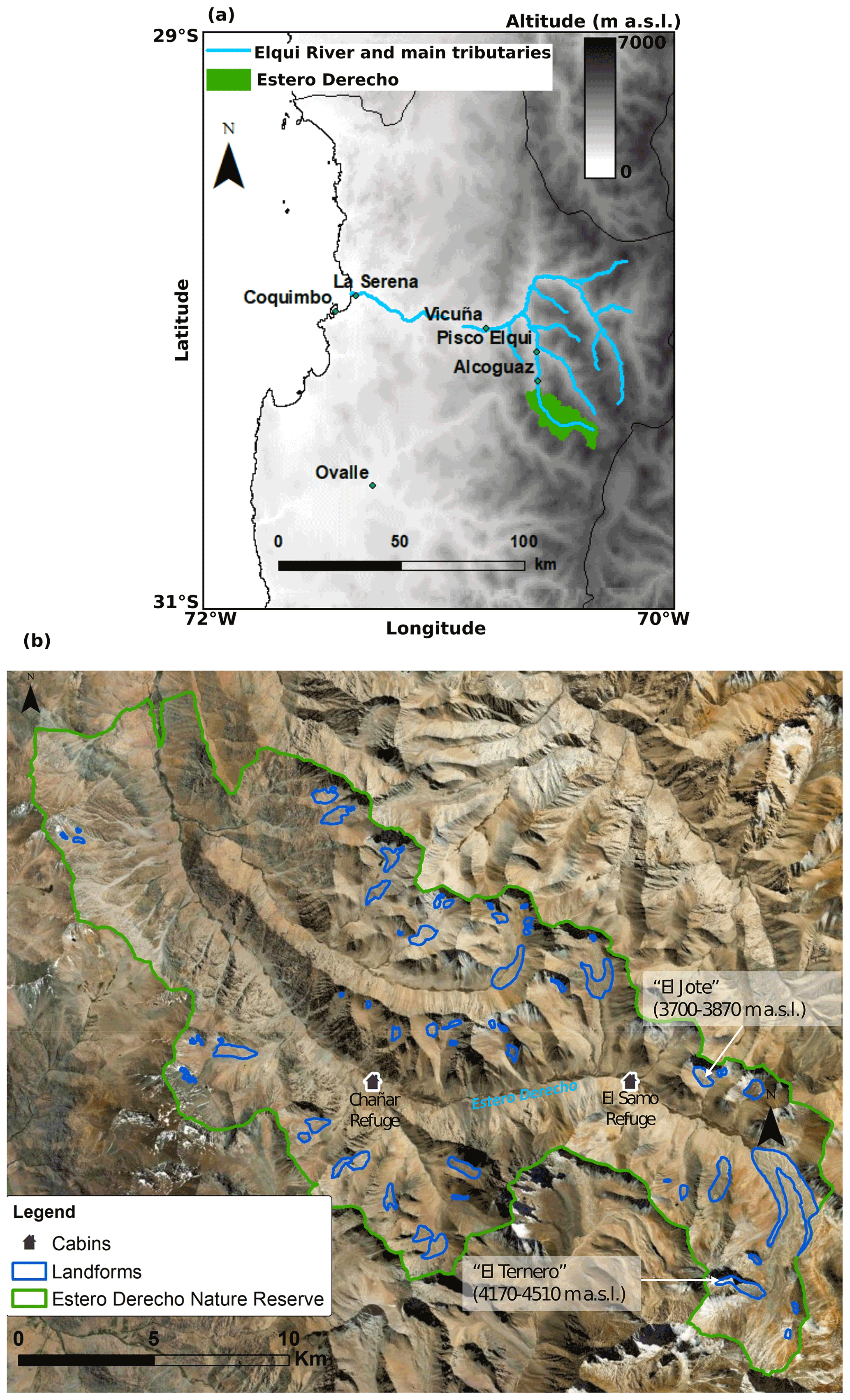
Figure 1 (a) Overview map indicating the location of Estero Derecho (∼30^∘ S, 70^∘ W) in the Coquimbo Region of Chile. Elevation map from the Advanced Spaceborne Thermal Emission and Reflection Radiometer Global Digital Elevation Model (ASTER GDEM). (b) Detailed map of Estero Derecho with an inventory of landforms created by the Centro de Estudios Avanzados en Zonas Áridas (CEAZA). The delineations for El Jote and El Ternero were created specifically for this study from the Esri base map satellite imagery. Both landforms are labelled with their respective elevation ranges.

The study site is within the semi-arid Andes of Chile at the southern edge of the Arid Diagonal and Atacama Desert (Sinclair and MacDonell, 2016). Specifically it is located at the headwaters of the Elqui River within the Coquimbo Region in a nature reserve called Estero Derecho (Fig. 1b). In the city of La Serena on the coast the annual precipitation is ∼90 mm a⁻¹ (average from 1981–2016; Valois et al., 2020b), drastically lower than the average annual precipitation for Chile of ∼1525 mm a⁻¹ (DGA, 2016). At the same time, demand from the agricultural sector, mining industry and municipal water supply are high, and water allocation has already been exhausted (DGA, 2016). Precipitation increases with elevation reaching ∼160 mm a⁻¹ at 2900 $\mathrm{m}\mathrm{a}.\mathrm{s}.\mathrm{l}.$ in the Estero Derecho valley (Valois et al., 2020b). Increased precipitation at higher altitudes allows for the formation of a seasonal snowpack that completely melts during the spring and summer seasons (Réveillet et al., 2020). Variability in precipitation at an inter-annual timescale is linked to El Niño–Southern Oscillation (ENSO; Favier et al., 2009), while at a decadal timescale it is linked to the Pacific Decadal Oscillation (Núñez et al., 2013). Precipitation has decreased since 1870 by ∼0.52 mm a⁻¹ at La Serena. The mean annual air temperature at a station at 3020 $\mathrm{m}\mathrm{a}.\mathrm{s}.\mathrm{l}.$ within Estero Derecho was 6.7 ^∘C between 2016–2020.

Within the nature reserve there are no debris-free glaciers, only rock glaciers and other periglacial landforms such as protalus ramparts and gelifluction lobes. The two rock glaciers assessed in this study are locally known as “El Jote” and “El Ternero” and are in the eastern part of the nature reserve (Fig. 1b) at 3700–3870 and 4170–4510 $\mathrm{m}\mathrm{a}.\mathrm{s}.\mathrm{l}.$, respectively. El Ternero is the largest intact rock glacier within Estero Derecho and has a lobate shape and clear flow features such as ridges and furrows, a steep frontal talus slope (∼40^∘) and well-defined lateral margins. There are a number of depressions ∼5 m deep on the surface and a pond on the surface covering an area of ∼80 m². El Ternero is 1.93 km long and has a maximum width of 0.51 km and an area of 0.60 km². It is deforming at a rate of ∼1 m a⁻¹ and lowering by ∼ 0.15 m a⁻¹ (based on three repeat differential GPS measurements taken in the summer of 2018–2019 and 2019–2020 between 4206–4417 $\mathrm{m}\mathrm{a}.\mathrm{s}.\mathrm{l}.$). In contrast, El Jote has poorly defined flow features and a moderately steep frontal slope (∼24^∘). This landform is stagnant according to unpublished repeat differential GPS measurements taken at five locations in the summer of 2018–2019 and 2019–2020. The lack of obvious flow features and its location within a cirque basin point toward the same conclusion. El Jote is 0.86 km long, has a maximum width of 0.48 km and covers 0.31 km². Its surface is characterized by lobes as well as signs of subsidence, such as depressions.

At El Ternero, a stream passes adjacent to the former and eroded terminal moraine. The waterway initiates on the mountain slope above and south of the rock glacier and continues downslope, eventually feeding a high-altitude wetland and the main waterway within the reserve, Estero Derecho. There is no evidence of water at the surface directly below the current frontal slope of the rock glacier. However, a substantial amount of water can be heard running below the rock glacier surface within topographic depressions. At El Jote, water emerges ∼200 m east of the main landform in a topographic low at ∼3740 $\mathrm{m}\mathrm{a}.\mathrm{s}.\mathrm{l}.$ It is unclear if this water originates from the rock glacier, another periglacial landform or a groundwater source. There is a small periglacial feature directly above that may be contributing, but no other obvious surface water source is visible. The waterway continues for ∼600 m, where it disappears ∼100 m below the frontal slope of the rock glacier. Water emerges in another, larger depression along the same flow path ∼550 m below the front of the rock glacier and continues downslope, contributing to an alpine wetland (i.e. bofedal) and Estero Derecho. There is vegetation adjacent to the water; in contrast there is little to no vegetation in the surrounding landscape.

3 Theory and methods

3.1 Geophysical measurements

Surface-based geophysical methods provide information about subsurface physical properties and have been extensively used to investigate the internal structure of rock glaciers (Hauck and Kneisel, 2008). In particular, electrical resistivity and refraction seismic tomography are common choices for the characterization of rock glacier internal structure, even though their use on irregular rock surfaces and frozen environments demands specialized techniques for sensor coupling and data acquisition.

3.1.1 Electrical resistivity tomography (ERT)

ERT collects information about the subsurface distribution of electrical resistivity (ρ) by injecting direct electric currents (DC) into the ground and measuring electric voltages at different locations. Data are obtained using a large number of resistance measurements made from spatially distributed four-point electrode configurations (Binley and Kemna, 2005). The geometry of the current injection and potential electrode pairs are varied with typical set-ups involving many tens of electrodes and several hundred or thousand data points. These data are then inverted to compute the spatial distribution of electrical resistivity in the subsurface (Dahlin, 1996).

Electrical resistivity quantifies the current density flowing through a cross-sectional area along a given length. In most rocks and soils, electrical current is carried by movements of ions in the pore water (electrolyte conduction) and by the movement of mobile ions in an electrical diffuse layer at the grain–fluid interface (surface conduction; Revil and Glover, 1997), with the mineral matrix generally characterized by high resistivity, unless electrical conductors are present within it (Lesmes and Friedman, 2005). Due to the high contrast in resistivity between saturated and unsaturated sediments and the marked increase in resistivity values at the freezing point, resistivity techniques have been useful in both hydrology (de Lima, 1995; Daily et al., 1992; Valois et al., 2018a, b) and permafrost studies (Evin et al., 1997; Hauck et al., 2003; Langston et al., 2011). In periglacial environments, the use of ERT is particularly popular due to the contrasting electrical resistivity corresponding to lithological media, water (high conductivity) and ice (low conductivity). Relevant values for electrical resistivity in rock glacier environments may be found in Maurer and Hauck (2007) and Hauck and Kneisel (2008).

The main limitation for ERT is the need for the electrodes to have a good galvanic contact with the ground. Its application within the surveys was therefore problematic due to the extremely high contact resistance caused by air pockets between the electrodes and the ground surface. Following the methodology of Maurer and Hauck (2007), we attenuated this problem by both facilitating the injection of electric current into the ground by attaching sponges soaked in saltwater to the electrodes and, in addition, increasing the measured voltage by implementing the Wenner–Schlumberger array configuration (its low geometrical factor provides larger measured voltages compared to other options).

3.1.2 Refraction seismic tomography (RST)

RST is based on the analysis of first arrival travel times of critically refracted seismic waves to reconstruct seismic P-wave (i.e. compressional-wave) velocity models (Nolet, 1987; White, 1989). When seismic waves impinge on velocity boundaries, they change their direction of propagation. At a critical angle that depends on the velocity contrast, head waves are created that move along the interface at the speed of the faster lower-lying layer velocity, and refracted waves are emitted. These refracted waves measured by the receiver and the timing of their arrival (i.e. first-arrival travel times) are the main observations used in seismic refraction surveys.

Seismic velocity is the rate at which seismic waves propagate through rocks and soils, and this generally increases with material density. In periglacial environments the different velocity values expected for lithology and ground ice (Maurer and Hauck, 2007; Hauck and Kneisel, 2008) is favourable for the application of RST. For this reason seismic refraction has been successfully used on rock glaciers since the 1970s (Barsch, 1971; Potter, 1972). In the last 2 decades the method has been extensively utilized in permafrost studies (Vonder-Mühll et al., 2002; Hauck et al., 2004; Draebing and Krautblatter, 2012) and to monitor hydrodynamic-variation impacts on velocities (Valois et al., 2016).

One limitation of first-arrival refraction methods is that they only use a small portion of the information contained in the seismic traces and strongly depend upon the assumption that velocity increases with depth. In the case of velocity inversion (i.e. the deeper medium presenting a lower P-wave velocity than the overlaying one), the refracted wave will bend towards the normal. This gives rise to the so-called “hidden-layer” phenomenon (Banerjee and Gupta, 1975). In addition, surface conditions on rock glaciers highly attenuate seismic energy and make it difficult to couple geophones and seismic sources to the ground. During the collection of seismic data, we were able to partially improve the coupling through the use of a few geophones fastened to metal plates. We also increased the signal-to-noise ratio by repeating the same source position five times.

3.2 Acquisition strategy

Field data collection was conducted during the austral summer between the end of January and the beginning of February 2020. The location of sensors and sources of all the profiles were taken with a Trimble differential GPS. At both sites, we acquired the ERT surveys using a Syscal Junior Switch-48 (IRIS Instruments, France) with 48 electrodes spaced 5 m apart and a Wenner–Schlumberger configuration with 23 levels at its maximum; the dipole lengths for the potential measurements were 5, 25 and 45 m, while for the current injections these were between 15 and 235 m with intervals of 10 m. For the El Jote rock glacier, the profile length was 690 m (Fig. 2a and b) and was obtained using five sequential roll-alongs in which 50 % of the electrodes stayed in place each time and the other 50 % were displaced along the profile line (Fig. 2e). In total we implemented 144 different electrode positions and obtained 2135 measurement points. For El Ternero the profile length was 575 m (Fig. 2c and d), which was obtained with four sequential roll-alongs. Here we used 120 different electrode positions and obtained 1479 measurement points. We recorded the refraction seismic surveys on both rock glaciers implementing a Geode Exploration Seismograph device (Geometrics, USA) along the same lines as for the ERT profiles. The seismic source was a 15 kg sledge hammer on a steel plate, and we repeated each shot position (stacking) five times in order to improve the signal-to-noise ratio. For the profile taken on El Jote, we used 48 geophones with a spacing of 5 m and shots in between geophone positions, but these were spaced 10 m apart. To obtain the length of 690 m, we applied five sequential roll-alongs as done for the resistivity line.

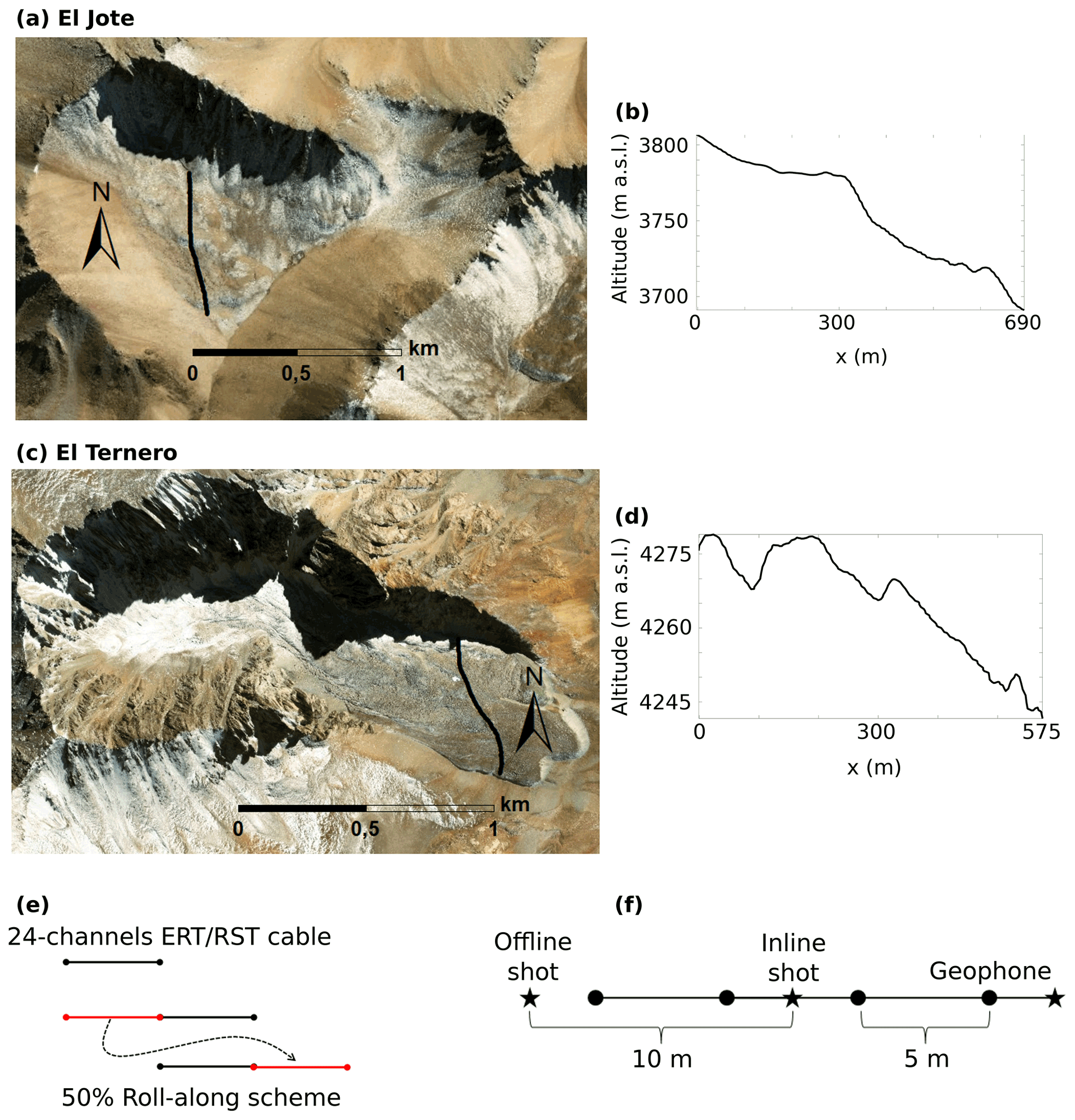
Figure 2 (a) Aerial image of El Jote showing the location of the geophysical survey line and (b) its topography from field differential GPS measurements. (c) Aerial image of El Ternero showing the location of the geophysical survey line and (d) its topography from field differential GPS measurements. Base maps in (a) and (c) from Esri World Imagery (2018). (e) Scheme of the 50 % roll-alongs used for ERT surveys on both rock glaciers and RST surveys on El Jote. (f) Scheme of geophones and inline/offline shot positions for RST surveys.

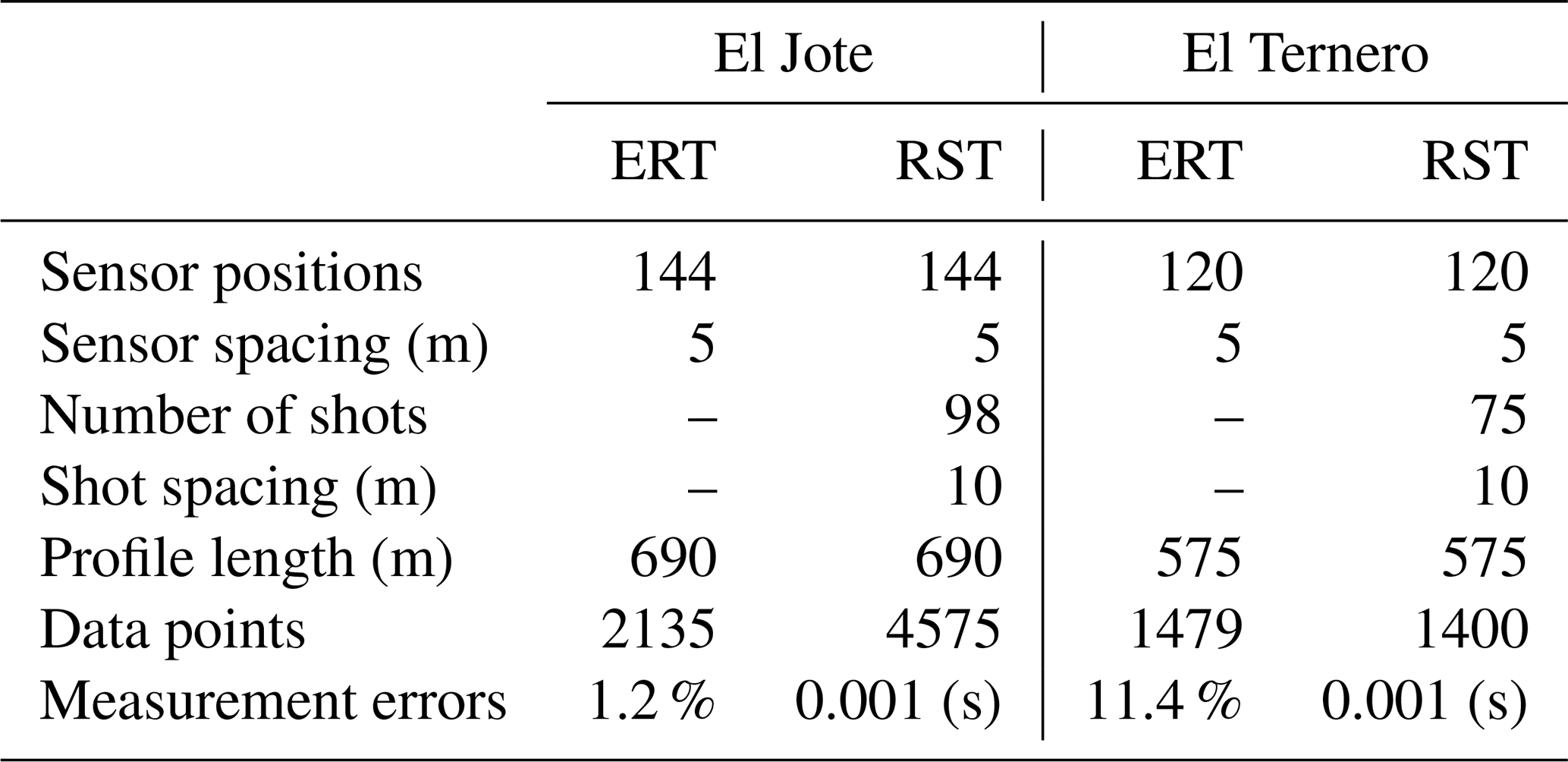
In the case of El Ternero, the same spacing and configuration was used for both shots and geophones, but after the first line, the failure of one of the cables reduced the number of geophones to 24. The total length of 575 m was then obtained by moving the 24-channel set-up four times and adding offline shots (Fig. 2f) to link the different acquisitions at distances of 5, 15 and 25 m from the last geophone at each end of the cable. While the geophysical line extended a bit past the edge of the El Jote rock glacier, it was impossible to do so in El Ternero because of the steep slopes of rock glacier edges, causing the access to be too dangerous. Collection of the profiles on El Ternero was logistically more challenging than on El Jote, due to higher altitudes, the extremely heterogeneous surface and especially the failure of one of the geophone cables. The overall data quality for this rock glacier is much lower than for El Jote (Figs. 4a and b and 6a and b). There are fewer data points, as measurements were not conducted for areas with high contact resistance in the case of ERT (almost 1.5 times less than for El Jote), and many traces were too noisy to identify the first arrival travel times for RST (more than 3 times less than for El Jote). For both profiles, we manually picked the first arrival travel times on each trace, resulting in 4575 picks for El Jote and 1400 for El Ternero. For the ERT observations, the error models resulted in 1.2 % relative error for El Jote and 15 % error for El Ternero; in the first case, the error was obtained from the average of the standard deviation for measured apparent resistivities, whereas in the second case such an average resulted in 11.4 %, but it was subsequently inflated to obtain a satisfactory inversion convergence. For the RST, an absolute error of 0.001 s was considered, as estimated from the average variability in the first arrival picking. The acquisition settings are summarized in Table 1.

Table 1 Acquisition settings for ERT and RST profiles on El Ternero and El Jote.

3.3 Data processing and inversion

The ERT observations were automatically filtered using the acquisition software for a standard deviation larger than 25 %, while for the seismic refraction travel time, we manually picked the first arrivals after applying a gain to the seismic traces; therefore the traces were filtered according to our ability to identify the first arrival times.

The inversion algorithms used to interpret the geophysical observations are part of pyGIMLi, an open-source library developed in Python for geophysical inversion and modelling (Rücker et al., 2017). On each rock glacier we implemented the same discretization mesh (with a maximum cell size of 400 m² at the edge of the ERT secondary mesh, and boundary conditions set to 4 times the span of the sensors) for both ERT and RST inversion routines and used a regularization weight of λ=10 for the inversion of all the datasets, which were chosen according to the L-curve analysis (Hansen, 2001). A schematic plot of the L-curve analysis for each collected dataset is given in Fig. 3. In all cases we present the model solution L2 norm against the residual L2 norm obtained for λ=1, 5, 10, 15, 50 and 100. We used a homogeneous resistivity starting model for both rock glaciers, with a value equal to the median of the apparent resistivities (${\mathit{\rho }}_{\mathrm{a}}^{\text{median}}=\mathrm{4561}$ Ω m for El Jote and ${\mathit{\rho }}_{\mathrm{a}}^{\text{median}}=\mathrm{36}\mathrm{054}$ Ω m for El Ternero) and a gradient model for the seismic velocity, starting with 300 m s⁻¹ at the top of the tomogram and gradually increasing to 5000 m s⁻¹ at the bottom. In each case, we refer to the error-weighted chi-square fit, where χ²=1 signifies a perfect fit (Günther et al., 2006), to quantify the resulting model parameters' ability to explain the field observations.

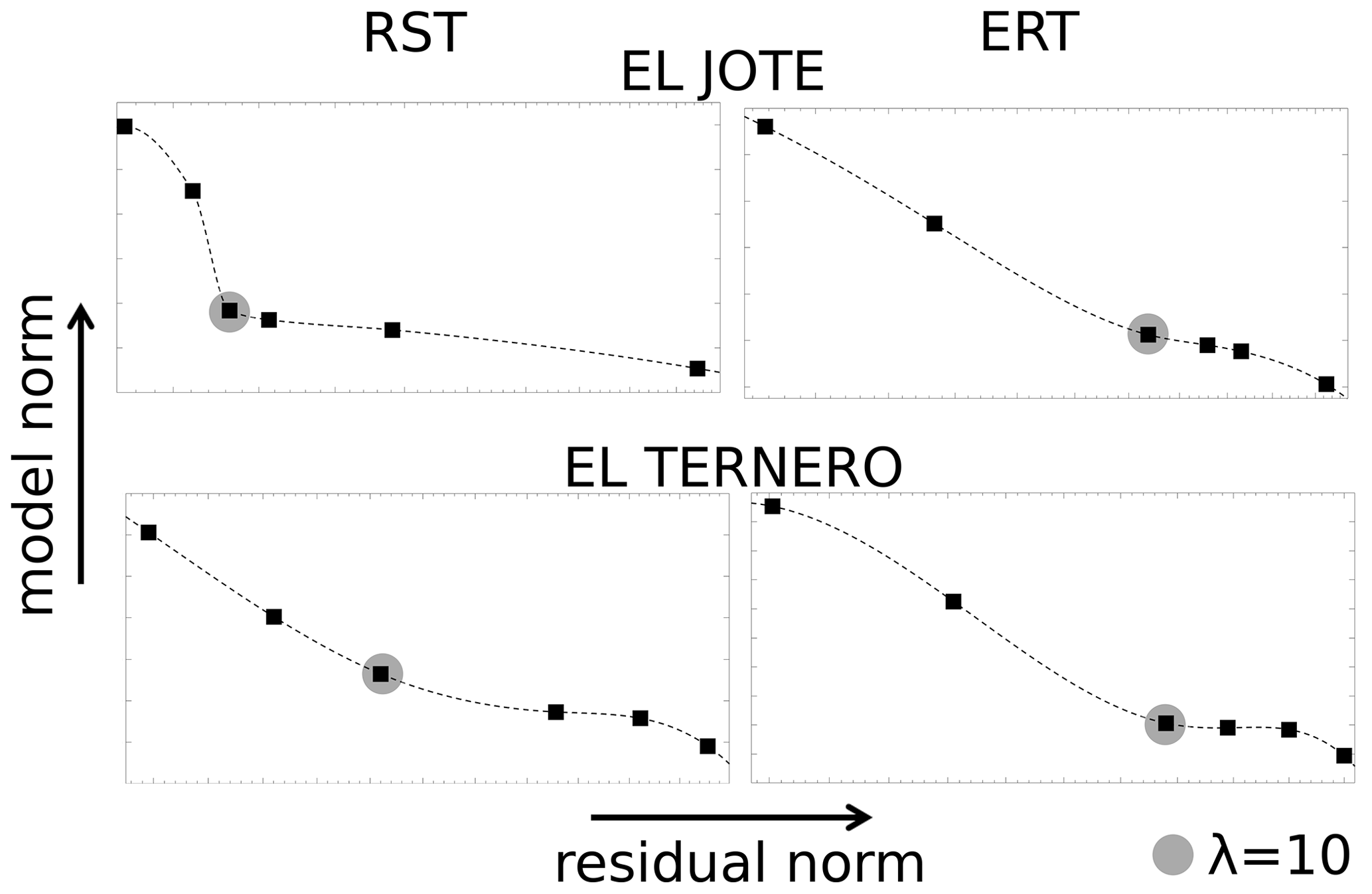
Figure 3 L-curve analysis for the regularization weights (λ) used in the inversion of ERT and RST data on both rock glaciers. In each plot, the values tested are λ=1, 5, 10, 15, 50 and 100.

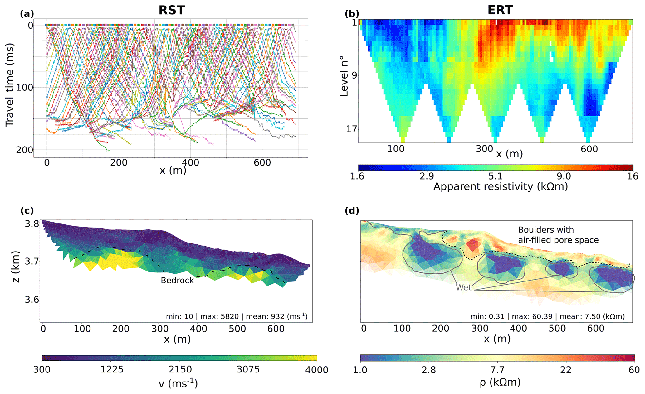
Figure 4 Geophysical observations and inversion model results for the El Jote rock glacier. (a) RST first arrival travel times. (b) ERT apparent resistivity. (c) Velocity and (d) resistivity tomograms. The velocity model is cut below the lowermost ray path, while the resistivity model transparency is proportional to the ERT data coverage. The velocity colour bar is linear, while the resistivity one is expressed in logarithmic scale.

In addition, to quantify the volumetric percentage of water, ice, air and rock within each of the two rock glaciers, we used the algorithm from Wagner et al. (2019) and tested in Mollaret et al. (2020) when implementing the four-phase model. For this inversion scheme we kept the same discretization meshes used for the individual inversions. The methodological details regarding this inversion algorithm and its application for this case study are given in Appendix A.

4 Results

4.1 El Jote

Figure 4 displays the datasets for (a) refraction seismic and (b) electrical resistivity tomography collected on the El Jote rock glacier, together with the (c) velocity and (d) resistivity tomograms obtained from their individual inversion. After 15 iterations we obtain a χ² of 1.43 for the ERT and 1.38 for the travel time data. At the top of the parameter domain the model results show low velocity (v<10³ m s⁻¹) and high resistivity (ρ>10⁴ Ω m), notably at approximately 300 m along the profile line, where the high resistivity values are concentrated and velocities are at a minimum. We interpret this layer as blocks and highly fractured rocks with air-filling pore spaces. This is consistent with field observations, where boulders are visible at the surface and possibly extend downwards along with fractured rocks until depths of 10 to 50 m. At the bottom of the tomogram the velocity model presents high velocity values between 150 and 250 m (between 50 and 80 m depth) and at approximately 550 m (between 40 and 50 m depth) along the profile line. In the first case the resistivity values are relatively low (ρ∼10³ Ω m), while at around 500 m they increase by 1 order of magnitude (ρ∼10⁴ Ω m). This increase can be explained by a decrease in air-filled pores, where between 150 and 250 m the pores are filled with water (generally characterized by lower resistivity than air-filled pores and particularly within frozen rocks, where water might be highly saline and therefore even more conductive; Jones et al., 2019), while near 550 m they are filled with ground ice (high resistivity), leading to changes in the surface conductivity at the grain–water or ice–water interface (Duvillard et al., 2018).

The results from the scheme of petrophysical joint inversion are presented in Fig. 5. These confirm the interpretation given for the individual inversion model and complement these results with the quantification of the volumetric content of the different subsurface components. The top layer (with a thickness varying between 10 and 50 m along the profile) is mostly air (up to 63 %; see Fig. 5e), with a low rock fraction (with a minimum of 27 % at the surface; see Fig. 5f). Below, the unconsolidated rocks are characterized by a decrease in porosity and relatively high content in water (up to 29 %; see Fig. 5c) except near the profile length of 550 m, where the ice content slightly increases to 3 % (Fig. 5d). The decrease in porosity could be explained by an increase in finer debris within this part of the rock glacier, which is gravity driven at larger depths and fill the pore space within larger-sized material. In addition, the high rock content at the bottom of the domain (88 %; see Fig. 5f) likely represents the top of the bedrock. Besides the similarity in the structure and component interpretation of the subsurface, the velocity and resistivity models (Fig. 5a and b) present differences if compared to the individual inversion results, with overall lower velocity values and higher contrasts in the resistivity values.

Figure 5 Results of petrophysical joint inversion of the El Jote field datasets. The tomograms represent (a) velocity- and (b) resistivity-transformed models. The directly inverted parameters are (c) water, (d) ice, (e) air and (f) rock volumetric content. All models are cut off below the lowermost ray path, with only the resistivity colour bar expressed in logarithmic scale.

4.2 El Ternero

Figure 6 displays the datasets for (a) refraction seismic and (b) electrical resistivity tomography collected on the El Ternero rock glacier, together with the (c) velocity and (d) resistivity tomograms obtained from their inversion. After 15 iterations we obtain a χ² of 1.49 for the ERT and 0.93 for the travel time data. The results show a thin layer (approximately 5±0.25 m thick) of low velocity and high resistivity which, as for El Jote, reflects the field observations, where boulders are visible at the surface of the rock glacier: unconsolidated rock with air-filled pore space. Below this layer, P-wave velocity increases gradually for the first 15–20 m up to v∼3000 m s⁻¹ and has a sharp increase at 25 m depth (v>4000 m s⁻¹). We interpret the gradual increase in velocity as a decrease in air-filled pores, which could be due to an increase in debris within the larger-sized materials (i.e. decreasing porosity), or as a gradual increase in compaction or ground ice, with sharp changes with either the presence of intact rock (i.e. top of the bedrock) or a significant increase in the amount of ground ice. Also, at approximately 150 and 450 m on the profile length the two low-value resistivity anomalies at depth most likely reflect the presence of water within the pore space. Likewise, at the surface low-resistivity anomalies are present within depressions at 80 and 260 m. The low-resistivity area at 450 m extends from the surface to the bottom of the profile.

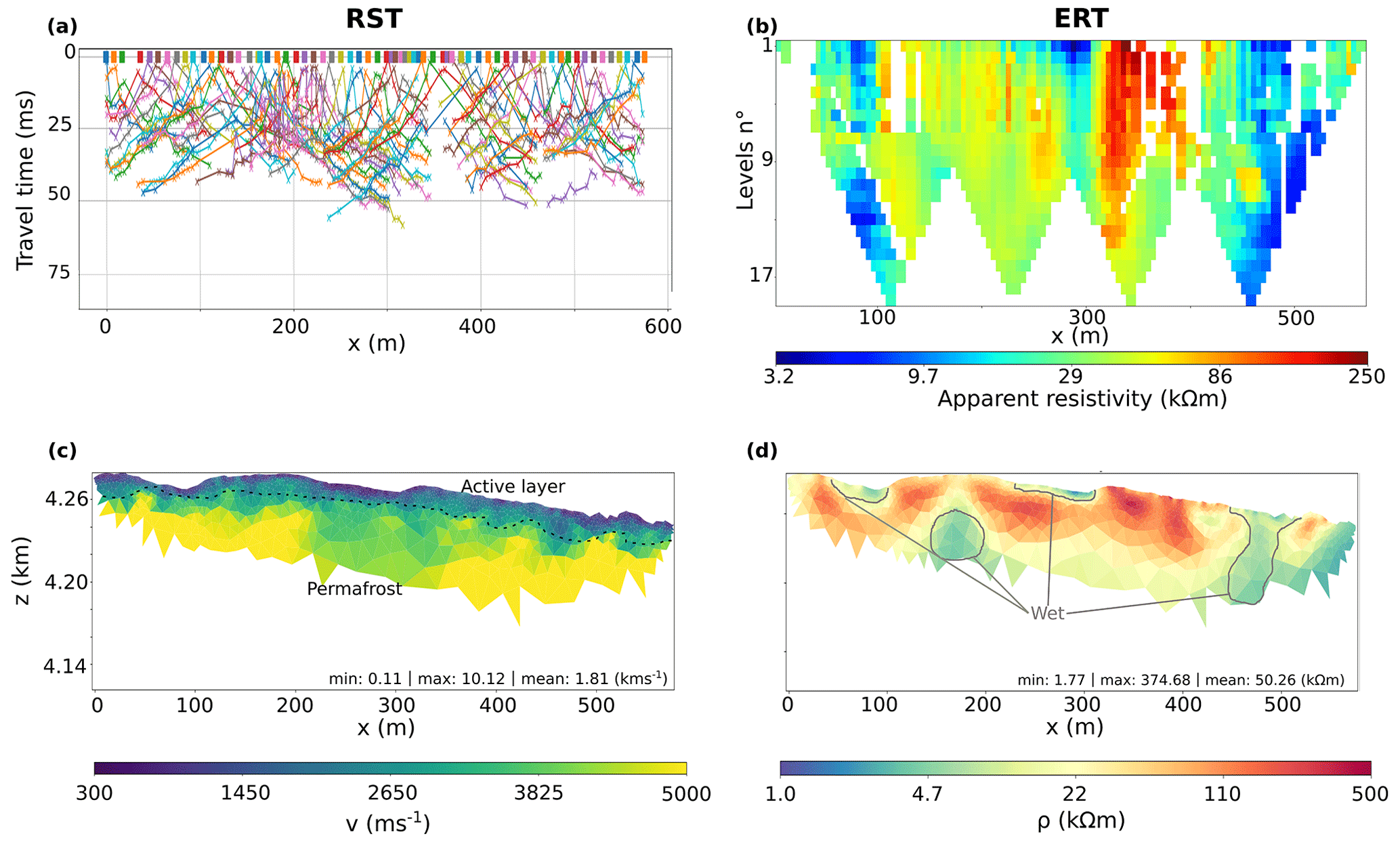
Figure 6 Geophysical observations and inversion model results for the El Ternero rock glacier. (a) RST first arrival travel times. (b) ERT apparent resistivity. (c) Velocity and (d) resistivity tomograms. The velocity model is cut below the lowermost ray path, while the resistivity model transparency is proportional to the ERT data coverage. The velocity colour bar is linear, while the resistivity one is expressed in logarithmic scale.

The joint inversion results obtained through petrophysical coupling (Fig. 7) provide a possible interpretation for the information gained through the comparison of the two individual inversion model results. Indeed, they confirm the presence of a thin top layer (approximately 5 m thick) with a moderately high fraction of air (up to 28 %; see Fig. 7e) overlaying a layer with a lower porosity and high ice content of more than 30 % for the majority of the model domain and up to 45 % at its highest concentration (Fig. 7d) except near the profile length of 150 and 450 m, where the fraction of water slightly increases to 13 % and 15 %, respectively (Fig. 7c). The low-resistivity areas at 80 and 260 m within depressions at the surface correspond to areas with elevated water fractions of 12 % and 13 %. As in the previous case, the velocity and resistivity models (Fig. 7a and b) present differences if compared to the individual inversion, with overall lower velocity and higher resistivity values and contrasts.

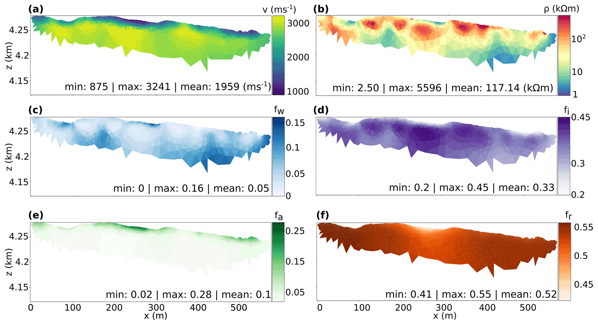
Figure 7 Results of petrophysical joint inversion of the El Ternero field datasets. The tomograms represent (a) velocity- and (b) resistivity-transformed models. The directly inverted parameters are (c) water, (d) ice, (e) air and (f) rock volumetric content. All models are cut off below the lowermost ray path, with only the resistivity colour bar expressed in logarithmic scale.

5 Discussion

5.1 Data quality and comparison of the inversion routines

For both field sites the acquisition of data and their quality were limited by the short time available and difficult terrain: the presence of large boulders with air-filled voids between them at the surface of both glaciers attenuated the propagation of both mechanical and electrical energy. The quality of the data was especially affected in the case of the El Ternero rock glacier, which is clearly demonstrated when comparing Figs. 4a and b and 6a and b. It must be stressed that the model parameter domains shown in the individual P-wave velocity inversion results and in the results of petrophysical joint inversion (Figs. 4c, 6c, 5 and 7) are geometrically delimited by the lowermost ray path, but there are poorly resolved areas in the P-wave velocity models presented due to the limited ray coverage within the displayed area. This limitation within the observations produces a major degree of uncertainty and ambiguity within the inversion model results that we try to address through the comparison of different inversion routines.

The overall structure of the inversion model results are largely consistent with the main patterns of high/low resistivities and high/low velocities presented in the individual inversion results, as these are preserved in the schemes of petrophysical joint inversion. This is also shown by the overall moderate to good correlation between the velocity and resistivity model results between the two inversion schemes, for both the El Jote (Fig. 8a with a correlation coefficient of 0.9 and Fig. 8b with a correlation coefficient of 0.6) and El Ternero rock glaciers (Fig. 8c with a correlation coefficient of 0.7 and Fig. 8d with a correlation coefficient of 0.5). Prior assumptions have a strong influence on inversion model results, and comparing the outcomes from different inversion schemes can help distinguish information contained within the data from artefacts due to different regularization and/or parametrization (de Pasquale et al., 2019). Therefore, the common distributions of relatively high and low values of resistivity and P-wave velocities between individual and petrophysical joint inversions are constrained by the data, since the two inversion schemes are based on different prior assumptions.

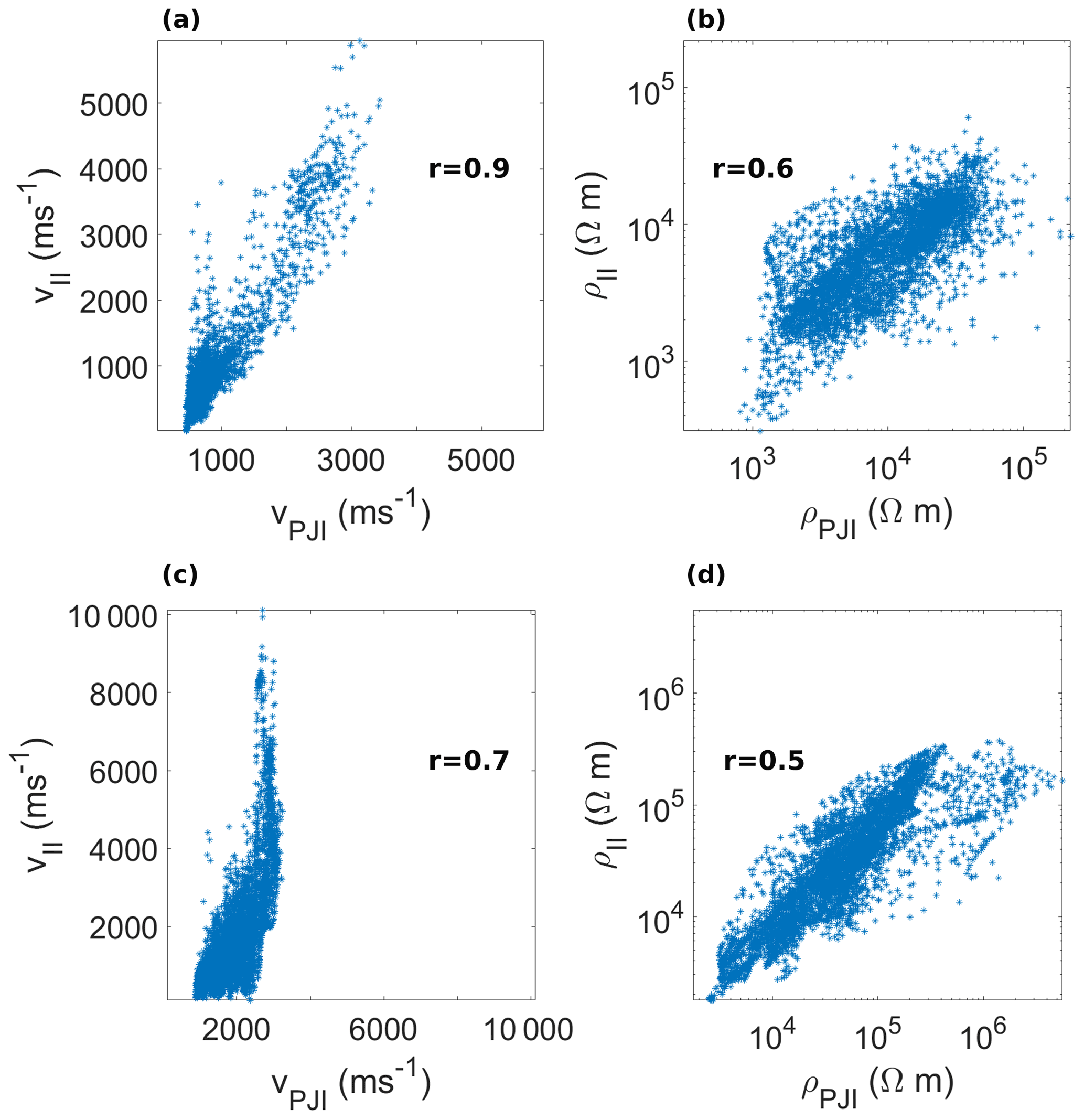
Figure 8 Correlation of P-wave velocity and resistivity model results between individual dataset inversion (II) and petrophysical joint inversion (PJI). El Jote P-wave (a) velocity and (b) resistivity model values. El Ternero P-wave (c) velocity and (d) resistivity model values. In each figure the correlation coefficient r is indicated.

Nevertheless, assessment of the numerical values of velocity and resistivity reveals some results we consider unrealistic and differences between the results from the two approaches. In the case of individual inversion results, P-wave velocity models (Figs. 4c and 6c) present some extremely low velocity values at the surface for El Jote (Fig. 8a; v_min∼ 10 m s⁻¹) and extremely high velocity values at the bottom of El Ternero (Fig. 8c; v_max∼10⁴ m s⁻¹). In the first case, the low values are compensated by a high-velocity anomaly at the bottom of the model which occupies a larger volume and has larger velocity values if compared with the results of the joint inversion routine (Figs. 8a and 5a). Instead for El Ternero, the high values are counterbalanced by lower velocity at the surface (v_min∼100 m s⁻¹) if compared with the results obtained through joint inversion routines (v_min∼900 m s⁻¹; Fig. 8c). Also, for both cases the results of petrophysical joint inversion present the smaller ranges of P-wave velocities (Fig. 8a and c) and the smoothest contrasts within the model, whereas the resistivity models give the highest values and sharpest contrasts within the model (Figs. 5b, 7b, and 8b and d). These discrepancies in the numerical values of resistivities and P-wave velocities are due to the different regularization used and to the choice of petrophysical relationships and parameters from which the physical properties are computed (Appendix A).

5.2 El Jote (relict rock glacier)

For El Jote, the results show a top layer (laterally variable between 10 and 50 m thick) of unconsolidated rock with air-filled pore space, especially from 300 m to the end of the profile line. This overlays a layer where the porosity decreases and appears saturated with water for the majority of the line, apart from near 550 m, where the fraction of ground ice slightly increases to 3 % (Fig. 5d). The increased velocity and resistivity at 550 m could also be interpreted as the presence of intact rock, as opposed to ground ice. As explained in Appendix A (Sect. A3), when the porosity of the subsurface is unknown, the scheme of petrophysical joint inversion does not easily differentiate between ice and rock content. In order to gain information about porosity, we unsuccessfully attempted to drill a core sample, but due to the hardness of rock at the site, the drill broke at very shallow depths. Nevertheless, for both inversion results we infer that within this rock glacier, it is likely that the ice has thawed, leaving behind large voids filled with air (top layer) or water (deeper layer). We classify El Jote as a relict rock glacier given that it contains little to no ground ice according to the geophysical results. For both the inversion results it seems that the bedrock is deeper than 100 m for almost the entire profile length. Also, at profile lengths of 150 to 250 m and approximately 550 m, the strong increase in velocity and resistivity values (Fig. 4c and d) and in rock content (Fig. 5f) at approximately 60 m depth may be interpreted as a shallower top of the bedrock. In addition, the lenses of lower resistivity values could be due to an increase in finer debris or water content within the pore space (ρ∼10³ Ω m), and the high water content in the bottom layer (more than 20 %) suggests the presence of an aquifer between the bedrock and the surface of the relict rock glacier. Also, the emergence of a perennial spring in a sloping peatland a few hundred metres below points towards the existence of a proglacial aquifer, which may be connected to the bodies saturated by rock glacier water. However, additional data are required to evaluate this hypothesis.

5.3 El Ternero (intact rock glacier)

The inversion model results for El Ternero are slightly shallower than those obtained for El Jote. This is due to the failure of one of the two geophone cables: the offline shots used to link the displaced arrays were recorded only by few of the closest geophones to the shot position, thereby losing ray coverage with depth. In addition, the low ray coverage at depth is also due to the poor signal-to-noise ratio for larger offsets. Nevertheless, we were able to retrieve useful information from the field measurements. The inversion outcomes show a 5 m thick active layer made of unconsolidated rock with air-filled pore space overlaying an ice-rich layer (Fig. 7d). Also, the steep increases in velocity values located between 10 and 25 m depth (Fig. 6d) most likely indicate rock compaction. Nevertheless this layer is not continuous, as there are low-resistivity anomalies near 150 and 450 m along the profile line which correspond to an increase in the water content (Fig. 7c), which could be a sign of local melting due to permafrost degradation or of reaching bedrock (and the bottom of the ice-rich layer).

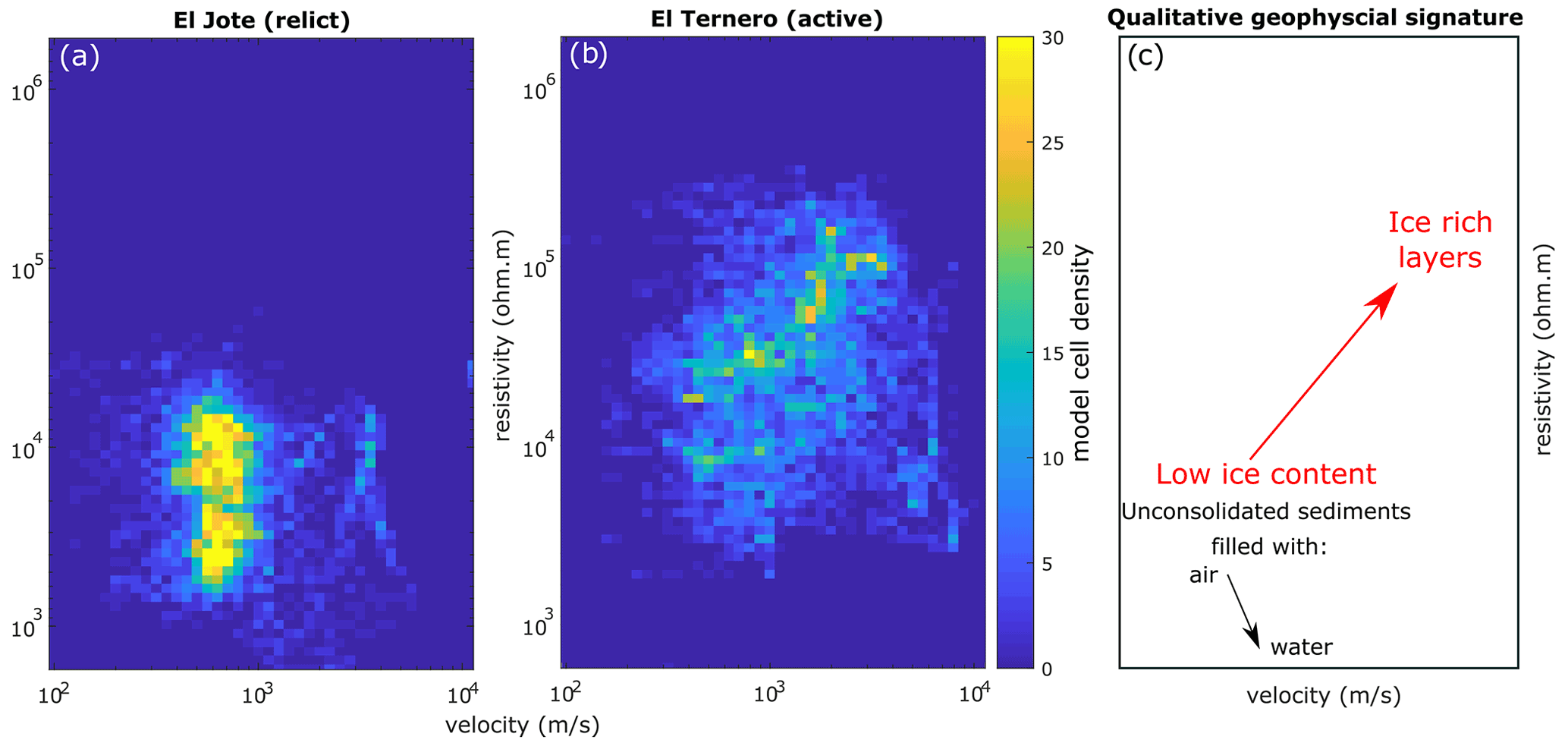
Figure 9 Density plots of resistivity versus P-wave velocity values for the (a) El Jote and (b) El Ternero datasets. (c) Schematic plot of the qualitative ERT and RST signature for intact and relict rock glaciers. The model cells involved in this analysis are inside the modelled grid, where there are ray paths and resistivity sensitivity.

Areas of lower resistivity and higher water content are observed in depressions between ice-rich permafrost zones on El Ternero at 80 and 260 m (Figs. 6d and 7c). A very similar pattern is observed on the Dos Lenguas rock glacier (Halla et al., 2021). We conclude, in agreement with Halla et al. (2021), that the ridge and furrow topography has an influence on surface hydrology of the rock glacier.

El Ternero has roughly the same seismic velocity range and maximum resistivity values as the Dos Lenguas rock glacier (Halla et al., 2021). The estimated average volumetric ice content for El Ternero of 33 % is very similar to the conservative estimate for Dos Lenguas of 32 % using the four-phase model (4PM; Hauck et al., 2011). The maximum ice content for Dos Lenguas is estimated to be 42 %–44 %.

5.4 Towards a diagnostic model representation for the ice presence in rock glaciers

The results from the petrophysical joint inversion help quantify the volumetric content of air, water, ice and rock and identify El Jote as a relict rock glacier and El Ternero as an intact rock glacier. However, in many cases the implementation of petrophysical joint inversion can be limited by the lack of proper petrophysical models (or parameters). When petrophysical model coupling is not possible, the comparison of velocity and resistivity model inversion results can still deliver substantial information about the rock glacier's internal structure. The resistivity–velocity density plots (Fig. 9) built from the individual model inversion results of Figs. 4c and d and 6c and d show clear differences between the two rock glaciers, with relatively low-resistivity and low-velocity clusters for the relict rock glacier, while the intact one is associated with higher velocities and resistivities.

The relatively low resistivities and low velocities (Fig. 9a) are in agreement with air-filled unconsolidated sediments inferred through the results of petrophysical joint inversion (Fig. 5e and f). The lowest resistivities may be associated with water and/or a proglacial aquifer (Fig. 5c; Sect. 5.2).

The gradual increases in resistivity and velocity (Fig. 9b) are evidence of solid material such as bedrock or ice-rich layers. Given the very high resistivities (over 10⁵ Ω m), our interpretation is that these are ice-rich layers, which agrees with the results of petrophysical joint inversion (Fig. 7d).

The rather different appearance of the two density plots (Fig. 9a and b) can be used as an indicator of the distinct nature of the two rock glaciers: overall, the relict rock glacier is characterized by lower resistivities and velocities, while the intact rock glacier is indicated by higher resistivity and velocity values, reflecting the ice-rich layer. The schematic plot (Fig. 9c) summarizes the findings for our two endmember rock glaciers and could be useful for identifying ice-rich landforms using methods of seismic and electrical resistivity.

The paper by Hilbich et al. (2021) is the only other publication we know of to complete a geophysical analysis comparing at least one active and inactive/relict rock glacier in the Andes. Our results show a similar pattern for resistivity–velocity plots of rock glaciers with maximum resistivity values <100 kΩ m in the case of an inactive/relict rock glacier (RGII), compared to those with maximum resistivity values >100 kΩ m in the case of an active rock glacier (RGI; Hilbich et al., 2021). Also, the mean values of resistivity and velocity for El Jote (7.5 kΩ m and 932 m s⁻¹ in the case of individual inversion) and El Ternero (50.26 kΩ m and 1810 m s⁻¹ in the case of individual inversion) fall well within the clusters associated with RGII and RGI rock glacier types in Hilbich et al. (2021). Finally, the ice volumetric content derived by Hilbich et al. (2021) through the four-phase model of the individual inversion results for RGI and RGII are similar to the ice volumetric content derived in this study for El Jote (0 %–3 %) and El Ternero (20 %–45 %) through petrophysical joint inversion.

6 Conclusion and outlook

In this study, we presented the comparison of geophysical signatures of one intact and one relict rock glacier using inversion results of refraction seismic and electrical resistivity tomography in the Chilean Andes. The obtained tomograms present much higher velocities and resistivities for the intact rock glacier, which we interpreted as a much higher ice content according to physical parameters for ERT and RST surveys on rock glaciers and the model results of petrophysical inversion.

The resistivity–velocity density plots show a clear signature difference between these rock glaciers, which makes sense given that El Jote is classified as a relict rock glacier with an aquifer below and El Ternero is an intact (active) rock glacier.

Through the joint interpretation of ERT and RST surveys for El Jote we were able to detect the top of the bedrock in part of the model domain and identify a potential aquifer, while in the case of El Ternero the active layer and the top of an ice-rich layer were identified, together with signs of its partial ground ice thawing at the bottom of the investigated area. The geophysical results confirm that El Ternero is an intact rock glacier with a significant amount of ice and that El Jote contains little to no ice (relict rock glacier).

There is ambiguity in the interpretation between the presence of ice or a rock matrix where resistivities and velocities are relatively high, especially for the El Jote inversion results. This could be improved adding information about subsurface porosity or by the incorporation of additional freeze–thaw sensitive datasets such as complex measurements of electrical resistivity (Wagner et al., 2019). In addition, to increase the investigated depth it would be necessary to improve the seismic data quality, which could be done by fastening the geophones to the surface by drilling small holes in the rock, although this would be logistically challenging.

Appendix A: Petrophysical joint inversion

Petrophysical coupling allows for the inversion of separate datasets to determine common parameters through petrophysical relationships. Within this framework, Wagner et al. (2019) developed an inversion scheme which allows for the interpretation of seismic refraction travel times and apparent resistivities in terms of ice, water, air and rock content. The inversion is based on a petrophysics four-phase model (4PM; Hauck et al., 2011) where partly or permanently frozen subsurface systems are assumed to be comprised of the volumetric fractions of the solid rock matrix (f_r) and a pore-filling mixture of water (f_w), ice (f_i) and air (f_a):

$$\begin{array}{}\text{(A1)}& f_{\mathrm{r}}+f_{\mathrm{w}}+f_{\mathrm{i}}+f_{\mathrm{a}}=\mathrm{1}.\end{array}$$

The treatment of the rock volumetric fraction as a single phase is a justified simplification in rock glacier environment, where the amount of sediments is negligible compared to the hard rock.

The volumetric fractions in Eq. (A1) are related to the seismic slowness (s), the reciprocal of the P-wave propagation velocity (v), through the time-averaging equation (Timur, 1968; Hauck et al., 2011) of

$$\begin{array}{}\text{(A2)}& s={\displaystyle \frac{\mathrm{1}}{v}}={\displaystyle \frac{f_{\mathrm{r}}}{v_{\mathrm{r}}}}+{\displaystyle \frac{f_{\mathrm{w}}}{v_{\mathrm{w}}}}+{\displaystyle \frac{f_{\mathrm{i}}}{v_{\mathrm{i}}}}+{\displaystyle \frac{f_{\mathrm{a}}}{v_{\mathrm{a}}}}\end{array}$$

and to the electrical resistivity through a modification of Archie's second law (Archie, 1942) of

$$\begin{array}{}\text{(A3)}& \mathit{\rho }={\mathit{\rho }}_{\mathrm{w}}(\mathrm{1}-f_{\mathrm{r}}{)}^{-m}{\left({\displaystyle \frac{f_{\mathrm{w}}}{\mathrm{1}-f_{\mathrm{r}}}}\right)}^{-n},\end{array}$$

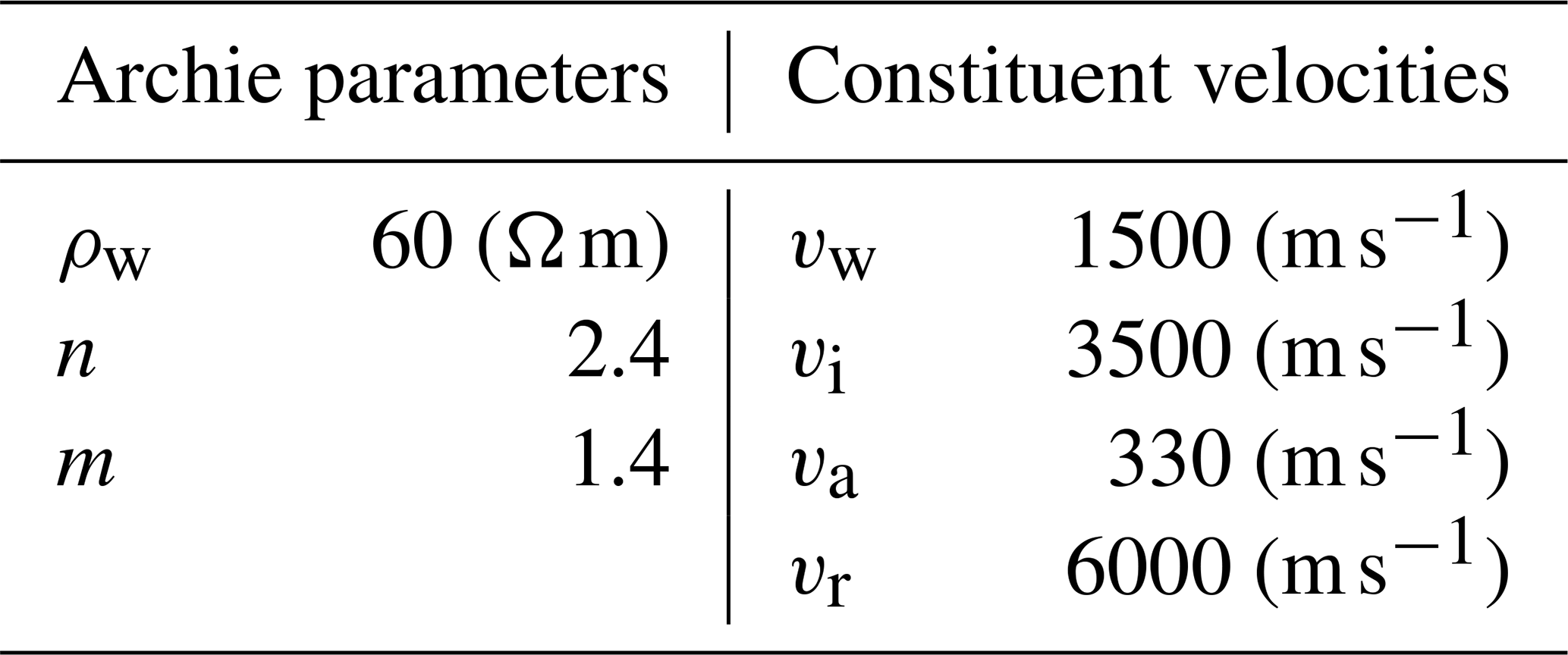
where the porosity is expressed in terms of rock content ($\mathit{\varphi }=\mathrm{1}-f_{\mathrm{r}}$) and m and n are the cementation and saturation exponents, which were set, respectively, to 1.4 and 2.4 after few trials, according to the minimization of χ². The assumptions within this 4PM model are that the medium is isotropic and has a single homogeneous mineralogy (validity of Eq. A2) and that the electric current flow is dominated by electrolyte conduction (validity of Eq. A3; Mavko et al., 2009).

The scheme of petrophysical joint inversion minimizes the following objective function (Wagner et al., 2019; Mollaret et al., 2020):

$$\begin{array}{}\text{(A4)}& \mathbf{\Phi }={\mathbf{\Phi }}_{\mathrm{d}}+\mathit{\lambda }{\mathbf{\Phi }}_{\mathrm{m}}+{\mathit{\lambda }}_{\mathrm{p}}{\mathbf{\Phi }}_{\mathrm{p}},\end{array}$$

where Φ_d refers to the combined data misfit, while Φ_m represents a smoothness regularization term built through four first-order roughness operators to promote smoothness in the distribution of each constituent of the four-phase system. The last term is an additional regularization term which constraints the volume conservation (Eq. A1). The two weights of λ and λ_p are responsible for scaling the influences of the two regularization terms, where λ is chosen to fit the data within the error bound and λ_p is chosen large enough to prohibit nonphysical solutions (i.e. with a sum of the four phases greater than 100 %).

Within this framework, the RST and ERT observations are used to infer the volumetric fractions of water, ice, air and rock for each model cell, while the spatial distribution of electrical resistivity and P-wave velocities are obtained through Eqs. (A2) and (A3), where the petrophysical parameters and constituent velocities are assumed to be spatially constant. We chose the values for the inversion of the field observations based on the literature (Hauck and Kneisel, 2008; Maurer and Hauck, 2007; Hauck et al., 2011; Wagner et al., 2019), which are listed in Table A1. Such parameters are appropriate for periglacial environments and consistent with relevant physical parameters for ERT and RST. Nevertheless, geotechnical in situ measurements could improve the estimation of those and therefore the accuracy of the inversion model results. A last important parameter to consider in this scheme is the porosity initial value and range. Wagner et al. (2019) already stressed the importance of a good porosity estimation in order to avoid ambiguity between ice and rock content, and in a recent study, Mollaret et al. (2020) analyse the influence of the porosity constraint in the results of petrophysical joint inversion. Following the approach of this last study and according to the previous knowledge from the field site, we tested different initial porosity values and ranges (ϕ_min–ϕ_max) for both rock glaciers. The choice was made by selecting the less constraining intervals which allowed for results consistent with the hypothesis of rock glacier formations and the surface geology of the two sites.

Table A1 Parameters used for the petrophysical joint inversion of the El Jote and El Ternero datasets (Eqs. A2 and A3).

A1 Inversion parameters for the El Jote and El Ternero rock glaciers

For both field locations we applied the same regularization weight as for the individual inversion, λ=10, while for ensuring the volume conservation, we applied λ_p=10 000. Regularization weights were chosen as illustrated by Mollaret et al. (2020), considering both classic L-curve analysis and the sum of the components fractions. For El Jote the initial porosity was set homogeneously to 30 % and inverted within a range from 0 % to 80 %, heterogeneously within the model. For El Ternero the initial porosity was set homogeneously to 60 % and inverted within a range from 10 % to 90 %, heterogeneously within the model. These values were tested as mentioned in the previous section with a maximum variation within the average volume contents of the inversion model results of 5 %. Also, we ran the petrophysical joint inversion for different combination of Archie's parameters (m and n) in order to minimize the χ². Few pairs of parameters led to comparably low χ² with values of m and n ranging, respectively, between 1.3 and 1.5 and between 2 and 2.5. These led to similar model results in terms of the volumetric contribution of the four phases and of the transformed resistivity and velocity values, with a principal effect on the water and ice content. For both rock glaciers we observed a slight decrease in water content (maximum of 4 % for El Jote and 3 % for El Ternero) and increase in ice content (maximum of 0.1 % for El Jote and 3 % for El Ternero) when n and/or m decreases. After 15 iterations we obtained an overall data fit corresponding to χ²=1.45 and χ²=1.26 for El Jote and El Ternero, respectively.

A2 Result uncertainties

We ran several numerical simulations in order to quantify the level of uncertainty on the petrophysical models obtained and check the ability of the measurement geometry to recover a realistic image of the subsurface. For both rock glaciers, we assumed the exact same settings as for the field surveys (i.e. same sensor locations, shot gatherings and quadrupole settings) and generated synthetic data from a known distribution of rock, air, water and ice. In Figs. A1 and A2 we show the synthetic models and the inversion model results calculated for the presence of data noise which equal the one modelled for the field measurements. For both synthetic models and inversion results, the directly modelled parameters are the water, ice, air and rock volumetric content, whereas the resistivity and velocity data are transformed following Eqs. (A2) and (A3). These are obtained assuming the same petrophysical parameters and constituent velocities as the one used for the inversion of the field data (Table A1).

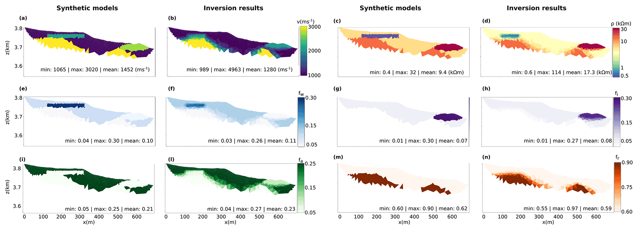
Figure A1 Synthetic models and results of petrophysical joint inversion for the El Jote field data settings. (a, b) Velocity- and (c, d) resistivity-transformed models. The directly modelled and inverted parameters are (e, f) water, (g, h) ice, (i, l) air and (m, n) rock volumetric content. All models are cut off below the lowermost ray path, with only the resistivity colour bar expressed in logarithmic scale.

Figure A2 Synthetic models and results of petrophysical joint inversion for the El Ternero field data settings. (a, b) Velocity- and (c, d) resistivity-transformed models. The directly modelled and inverted parameters are (e, f) water, (g, h) ice, (i, l) air and (m, n) rock volumetric content. All models are cut off below the lowermost ray path, with only the resistivity colour bar expressed in logarithmic scale.

In Fig. A1, we present the model and inversion results obtained for the same field settings as implemented on El Jote. In the case presented, the relative error on the ERT-simulated measurements was set to 1.2 %, and the absolute error on the RST data was set to 0.001 s. The resulting model error (ME) for each parameter (M; e.g. air, water, rock and ice contents and resistivity and velocity values) was than computed as

$$\begin{array}{}\text{(A5)}& \text{ME}={\displaystyle \frac{|{\mathit{M}}_{\text{inv}}-{\mathit{M}}_{\text{syn}}|}{{\mathit{M}}_{\text{syn}}}},\end{array}$$

where inv and syn refer to the inverted and synthetic model parameters, respectively. The average model error obtained was of 28 % for the air content, 16 % for the ice content, 23 % for the water content, 7 % for the rock content, 30 % for the interpreted velocity and 21 % for the interpreted resistivities. Structurally, it is possible to observe that the surface water anomaly modelled between ≈100 and 300 m of the profile length is much smaller in the case of the inversion results. This is due to the low ray coverage in this area and the lack of a sufficiently large number of quadrupoles within the field measurements. Nevertheless, the inverted results show the ability of the measurements taken to resolve water and ice anomalies, together with the bedrock interface, once the proper data error is modelled. In fact, when we tried to increase/decrease the error level set within the inversion routine (while keeping the same noise in the synthetic data), the model uncertainties increases significantly (by ≈30 % when the error is set to 1 % for ERT and 0.0005 s for RST and by ≈40 % when the error is set to 5 % for ERT and 0.002 s for RST).

In the case of El Ternero (Fig. A2), we focus on the ability of the field measurements to resolve the interfaces of the active layer and bedrock. In this case, the relative error on the ERT-simulated data was set to 12 %, and the absolute error on the RST data was set to 0.001 s. The average model error resulted in 24 % for the air content, 41 % for the ice content, 32 % for the water content, 10 % for the rock content, 39 % for the interpreted velocity and 23 % for the interpreted resistivities. Even though the volumetric quantities present some differences between the synthetic model and inversion results, the interfaces between active and inactive (ice-rich) layers and the bedrock surfaces can be retrieved from the inversion model results. As for the El Jote field measurement settings, the increase/decrease in the error level within the inversion routine led to an increase in the model uncertainties (by ≈31 % when the error is set to 6 % for ERT and 0.0005 s for RST and by ≈39 % when the error is set to 20 % for ERT and 0.002 s for RST).

A3 Methodology limitations

Within their study, Wagner et al. (2019) applied the scheme of petrophysical joint inversion to two synthetic test cases and an Alpine field site. They emphasized the need for a good porosity estimation/knowledge in order to reduce the ambiguity between rock and ice content. Such ambiguity was already stressed by Hauck et al. (2011), where the analytical exploration of the range of possible values for ice, water, air, and rock contents for a given pair of resistivity and velocity values show that air and water content can be discriminated quite well even if porosity is unknown, while there is a strong ambiguity between ice and rock contents. This limitation comes from the similar resistivity and P-wave ranges that characterize both the ice and rock matrix, which results in a wide range of possible porosities. Nevertheless, Mollaret et al. (2020), who applied the methodology of Wagner et al. (2019) to five different Alpine field sites, found that the methodology is applicable for very different permafrost landforms, with ice contents varying from low to high volumetric contents, and that rock and ice contents are best resolved when the measured P-wave velocity is relatively low or high. In their study, Mollaret et al. (2020) also implemented four different petrophysical models of electrical resistivity: Archie's law, Archie's law with a surface conduction, a surface conduction model and a geometric mean model. They show that in the first three cases the inversion results are largely comparable and depend on the porosity estimation, although they are based on theoretically different electrical conduction processes (due to the lack of field calibration of the respective electrical material parameters included in the equations so that these parameters are similarly determined by minimizing the data misfit). In contrast, when using the geometric mean model, the sensibility to porosity estimation decreases but is computationally more demanding due to the need for finding combinations of the four-phase resistivities for inversion to convergence. To avoid increasing the number of unknown constants within the inversion routine (i.e. the resistivities of the four phases), we decided to apply Archie's law as a petrophysical model of electrical resistivity (Eq. A3).