Snow water equivalent change mapping from slope-correlated synthetic aperture radar interferometry (InSAR) phase variations

Area-based measurements of snow water equivalent (SWE) are important for understanding earth system processes such as glacier mass balance, winter hydrological storage in drainage basins, and ground thermal regimes. Remote sensing techniques are ideally suited for wide-scale area-based mapping with the most commonly used technique to measure SWE being passive microwave, which is limited to coarse spatial resolutions of 25 km or greater and to areas without significant topographic variation. Passive microwave also has a negative bias for large SWE. Another method is repeat-pass synthetic aperture radar interferometry (InSAR) that allows measurement of SWE change at much higher spatial resolution. However, it has not been widely adopted because (1) the phase unwrapping problem has not been robustly addressed, especially for interferograms with poor coherence, and (2) SWE change maps scaled directly from repeat-pass interferograms are not an absolute measurement but contain unknown offsets for each contiguous coherent area. We develop and test a novel method for repeat-pass InSAR-based dry-snow SWE estimation that exploits the sensitivity of the dry-snow refraction-induced InSAR phase to topographic variations. The method robustly estimates absolute SWE change at spatial resolutions of < 1 km without the need for phase unwrapping. We derive a quantitative signal model for this new SWE change estimator and identify the relevant sources of bias. The method is demonstrated using both simulated SWE distributions and a 9-year RADARSAT-2 (C-band, 5.405 GHz) spotlight-mode dataset near Inuvik, Northwest Territories (NWT), Canada. SWE results are compared to in situ snow survey measurements and estimates from ERA5 reanalysis. Our method performs well in high-relief areas, thus providing complementary coverage to passive-microwave-based SWE estimation. Further, our method has the advantage of requiring only a single wavelength band and thus can utilize existing spaceborne synthetic aperture radar systems.

1 Introduction

Snowmelt is one of the greatest sources of water in snow-affected areas (Barnett et al., 2005), snow accumulation on glaciers is critical to their mass balance and longevity (Zemp et al., 2009), and snow cover variation is a dominant control on ground thermal regimes in cold regions (Mackay and MacKay, 1974); thus quantification of snowpack conditions is essential to understanding the role of snow on earth system processes. Snow water equivalent (SWE) is the amount of liquid water in a vertical column of snow and is a key parameter of snowpack conditions. The SWE of a snow layer is equal to the product of its depth and mean density. Traditionally, SWE variation over space and time is interpolated from sparse point-based measurements (Grünewald et al., 2010), which generally show significant spatial variation due to factors such as topography and vegetation (Anderton et al., 2004; Jost et al., 2007), as well as temporal bias if the acquisition of each set of points is distributed over a range of dates (Smyth et al., 2020). Ideally the SWE measurement is carried out over a short time span to limit within-set variation due to changing meteorological conditions. Further bias may be introduced if different point-based methods are integrated together to estimate SWE over large areas. To avoid biases arising from the interpolation of point-based measurements of typical snow packs, several remote sensing techniques have been developed for wide-scale, area-based determination of SWE. With precipitation regimes changing globally under persistent climate change (Pachauri et al., 2015), remote sensing techniques offer the potential to monitor hydrological conditions over vast areas of cold regions where point-based measurements are typically sparse and collected intermittently with a range of techniques.

Snow depth has been determined using surface elevation models developed using lidar, as well as structure-from-motion (optical photogrammetry) systems, either by differential repeat-pass measurement or comparison with a pre-existing snow-free reference elevation model (Deems et al., 2013; Nolan et al., 2015). However, as these systems are presently only feasible on airborne platforms they have not yet been used for repeated, wide-scale SWE mapping, which is required to substantively improve hydrological monitoring. Alternatively, spaceborne systems are designed for repeated wide-scale monitoring, and both passive- and active-microwave methods to determine SWE have been demonstrated (Saberi et al., 2020; Lemmetyinen et al., 2018). However, despite the potential for spaceborne microwave determination of SWE, there are key limitations inherent within each of the current approaches that affect the sensitivity and uncertainty of the measurements and prevent adoption of the methods for wide-scale SWE monitoring.

Passive-microwave SWE estimation is based on the measurement of the attenuation of Earth-emitted thermal microwave radiation by an overlaying snowpack (Kunzi et al., 1982). It has been implemented on several spaceborne systems, generating global SWE maps with a revisit frequency of up to daily (e.g., Takala et al., 2011). However, the passive-microwave method has severe limitations (Takala et al., 2011). These are as follows: (1) increased uncertainty for larger SWE (> 150 mm) due to attenuation saturation, (2) dependence on properties of snow microstructure, (3) signal contamination from topographic variation, which restricts the method to low-relief regions, and (4) coarse spatial resolution, e.g., > 25 km in the case of Advanced Microwave Scanning Radiometer (AMSR)–E daily products.

In contrast to passive systems, active-microwave SWE estimation methods are based on interpreting variation in backscattered radiation following interaction with the snowpack. One method that promises high spatial resolution is dual-frequency active microwave estimation, which measures total SWE in a single pass of a synthetic aperture radar (SAR) based on the difference between the volume backscatter power returned by the snowpack by two radio frequency bands (e.g., X-band vs. Ku-band). The dual-band requirement of this method currently limits it to ground-based and airborne implementations, although method-capable spaceborne missions have been proposed (e.g., Rott et al., 2012; Derksen et al., 2019). Limitations of this method include a dependence on snow microstructure and an applicability restriction to predominately dry-snow and vegetation-free areas (Oveisgharan et al., 2020).

Active-microwave-based estimation of dry-snow SWE change can also be achieved through repeat-pass SAR interferometry (InSAR) by exploiting the phase contribution that results from refraction in dry snow (Guneriussen et al., 2001; Deeb et al., 2011; Leinss et al., 2015). This method measures temporal SWE changes between repeat acquisitions rather than total SWE; the latter must be inferred later through integrating the SWE change maps over time. Performance depends on sensing frequency: higher frequencies (e.g., X-band compared to C- or L-band) have better phase sensitivity to SWE change but are more prone to temporal decorrelation and to interference from volume scattering. This method promises high spatial resolution, but it is constrained by the following requirements: (1) observability is limited to conditions in space and time with low decorrelation, (2) a spatial reference with known SWE change since the InSAR phase carries an unknown offset, and (3) phase unwrapping to resolve 2π ambiguities, which occur in significant number for typical snowpacks (Rott et al., 2003; Leinss et al., 2015). Decorrelation increases with liquid water content, changes in snow distribution, and volume scattering. Particularly, due to the need and difficulty of phase unwrapping, the method has not yet been operationally adopted for wide-scale, repeat monitoring of SWE despite being proposed and demonstrated over 20 years ago (Guneriussen et al., 2001).

Furthermore, polarimetric refraction-based methods have been proposed to exploit the structural anisotropy of snow to provide additional information about SWE change within a snowpack (Leinss et al., 2016, 2020), although in this article we focus on single-polarimetric methods.

The Delta-K method for SWE estimation (Engen et al., 2004) is a variant of the InSAR method that differences the InSAR dry-snow phase between two radar carrier frequency sub-bands. This approach has the benefits of not requiring a spatial phase reference and eliminates the need for phase unwrapping. However, these are at the cost of a much-reduced sensitivity that requires substantial spatial smoothing to suppress the noise, which results in only coarse spatial resolution SWE estimates. For example, Engen et al. (2004) report 100 mm accuracy at 10 km resolution when applying the method to European Remote-Sensing Satellite (ERS-1) (C-band) data.

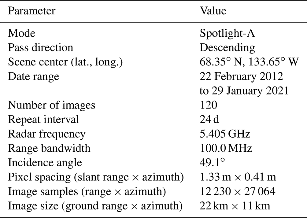
Table 1 Parameters for the RADARSAT-2 dataset used for this study.

We hypothesize that it is possible to overcome some of the key limitations of repeat-pass InSAR for dry-snow SWE change estimation, at the cost of only moderately reduced spatial resolution, by exploiting the sensitivity of the dry-snow refractive InSAR phase signal to topographic slope. Our objective is to develop a spatial analysis method for repeat-pass InSAR that allows for unambiguous SWE change estimation directly from the wrapped InSAR phase without the need for a spatial phase reference and phase unwrapping and that is insensitive to other InSAR phase components not correlated with topographic slope at the scale of the output resolution (size of SWE estimation window). Our method exploits the dependency of the refractive phase delay within the snowpack with respect to the local terrain slope. This novel method is conceptually similar to established methods for estimating temporal changes in the layered tropospheric delay in repeat-pass InSAR (e.g., Lin et al., 2010) and offers the same benefits as the Delta-K method but with substantially better sensitivity and spatial resolution for most terrains.

The proposed method was tested with a multi-year RADARSAT-2 dataset situated in the western arctic region of Canada. The study site was chosen for three primary reasons: (1) relatively long dry-snow season, (2) moderate topographic variation, e.g., more than flat prairie-like conditions but less than in an alpine region, and (3) dataset availability since an archived stack of 120 Spotlight images over 9 years is somewhat unusual and allows for detailed temporal analysis of results.

Our paper is organized as follows: first we describe the study site, SAR dataset, and ancillary data that we use to demonstrate and test the novel method. We then develop a quantitative model for the repeat-pass InSAR phase resulting from dry-snow refraction that explicitly considers topographic slope variation. Subsequently, we introduce a spatial-correlation-based method for estimating SWE change from a repeat-pass interferogram, first from a locally unwrapped spatial phase signal and then directly from the wrapped phase. We compare the expected performance and precision of our method to that of the Delta-K method. Next, we show results from applying our novel SWE retrieval method to the full RADARSAT-2 InSAR dataset. We compare these results to several in situ SWE transect surveys located within the imaged footprint, as well as the SWE temporal history estimated by the ERA5 climate reanalysis model. We then discuss sources of estimation error in our new approach and establish their relative significance. Sources considered include the effects of (1) violated model assumptions, (2) other InSAR phase components, and (3) digital elevation model (DEM) errors. Finally, we present our conclusions with a focus on the feasibility of our method for SWE change mapping in the context of existing methods.

2 Data

2.1 SAR dataset and study site

The InSAR dataset used for this study is a time series of 120 RADARSAT-2 Spotlight-A (RS2-SLA) descending-pass single-look complex (SLC) images spanning the period 22 February 2012 to 29 January 2021 at 24 d intervals, and it is nearly continuous with only a few time gaps (Table 1). The study area is situated in the Northwest Territories, Canada, at the eastern margin of the Mackenzie Delta, about 120 km south of the Beaufort Sea coast. It covers 238 km² defined by the SAR imaging footprint and includes the town of Inuvik. The mean backscatter amplitude image for the dataset is shown in Fig. 1a.

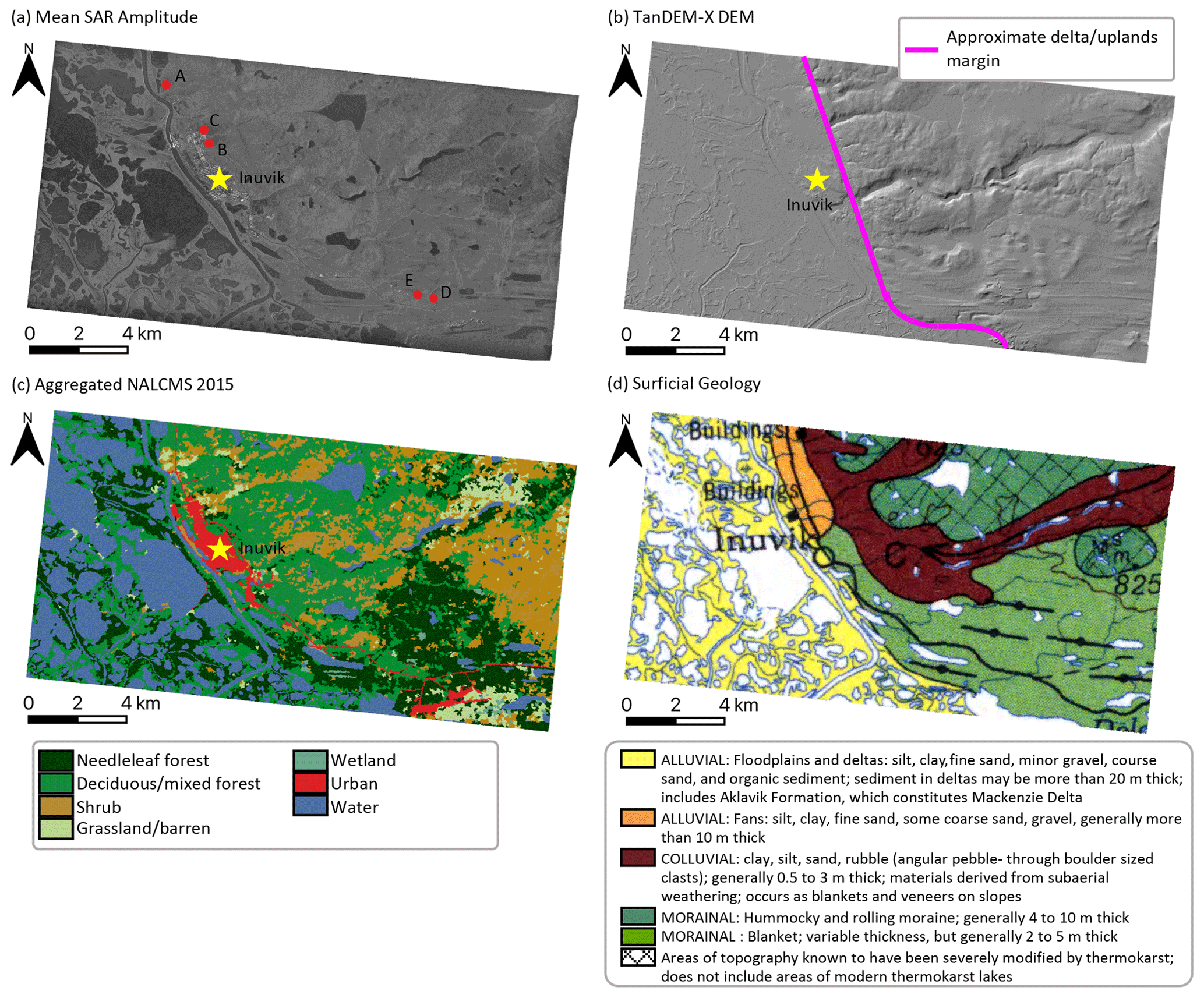
Figure 1 (a) Mean amplitude of all co-registered RS2-SLA images; (b) hill-shaded TanDEM-X DEM (DLR 2016) over the SAR footprint showing approximate margin between lowland delta area and the uplands east of the delta; (c) North America Land Change Monitoring System (2015) classification map (provided jointly by Natural Resources Canada, Comisión Nacional para el Conocimiento y Uso de la Biodiversidad, Comisión Nacional Forestal, Instituto Nacional de Estadística y Geografía, and the U.S. Geological Survey, 2015) aggregated into major land cover classes; (d) surficial geology map of the area from Rampton (1987). © Her Majesty the Queen in Right of Canada, as represented by the Minister of Energy, Mines and Resources Canada, 1987. Positions labelled A–E in panel (a) refer to the snow surveys described in Sect. 2.2.

Our proposed SWE change estimation method requires knowledge of the variation in topographic slope. To derive the slope, we used a 12 m spatial resolution TanDEM-X digital elevation model (DEM) provided by the German Aerospace Centre (DLR). This DEM was derived from source images acquired between 13 January 2011 and 8 August 2014 including snow-season acquisitions, so some snow-related bias may affect the estimated elevations. Regarding DEM accuracy, our method described in Sect. 3.3 depends on local slope variations and is therefore sensitive only to local relative rather than absolute DEM errors. Wessel et al. (2018) report a root-mean-square error (RMSE) of 1.8 m for TanDEM-X elevations over forested terrain. We also used this DEM for InSAR topographic phase correction and as an input for snow transport modelling, discussed in Sect. 5.2. The DEM shows that the Mackenzie Delta (near sea level) in the eastern portion of the study area has little topographic variation, but to the east of the delta's margin, elevation increases to a maximum of approximately 200 $\mathrm{m}\mathrm{a}.\mathrm{m}.\mathrm{s}.\mathrm{l}.$ (Fig. 1b). Several riparian zones drain this upland area towards the delta and create substantial local-scale topographic variation.

The study area is south of the treeline and ecologically is broadly categorized as subarctic boreal forest. However, according to the North American Land Change Monitoring System (NALCMS) 2015 dataset, which is a 30 m resolution land classification based on Landsat and RapidEye imagery using the methodology described by Latifovic et al. (2017), there is significant variation in vegetation classification within the study area (Fig. 1c). The upland area east of the delta features forest, shrubland, and grassland, whereas the delta proper is predominantly forested but is interspersed with areas of shrubs and sedge wetlands (Burn and Kokelj, 2009). There are 6.5 km² of developed lands in the study area that include the centrally located town of Inuvik, segments of the Inuvik–Tuktoyaktuk highway (ITH) and the Dempster highway that extend, respectively, northward and westward from the town site, and the Inuvik airport in the southeastern corner of the study footprint.

The study area lies within the (spatially) continuous permafrost region (Heginbottom, 1995; Nguyen et al., 2009). Permafrost is ground that remains at or below 0 ^∘C for 2 or more years that is overlain by an active layer that thaws seasonally. The permafrost in the study area is commonly ice-rich (Burn et al., 2009) and occurs within surficial deposits of several origins that are predominantly unconsolidated (Fig. 1d). As a result of climate warming in the region, permafrost temperatures and active layer thickness are increasing and producing ground surface settlement where there is net thaw of near-surface, ice-rich permafrost (Kokelj et al., 2017; O'Neill et al., 2019).

As shown in Fig. 2, Inuvik normally receives some level of snowfall for all months of the year except July (ECCC, 2021a). The mean annual snowfall is 1586 mm. For dry-snow conditions, temperatures must remain below freezing; the daily maximum temperatures in Inuvik normally remain below zero for the months of October to April. At upland locations, dry snow in the area is redistributed by wind, and large drifts develop in relation to topographic relief and shrub growth, while in the delta proper, forest and shrub vegetation combine with the lack of relief to minimize wind effects on the snow pack (Burn et al., 2009; Mackay and MacKay, 1974; Palmer, 2007; Morse et al., 2012).

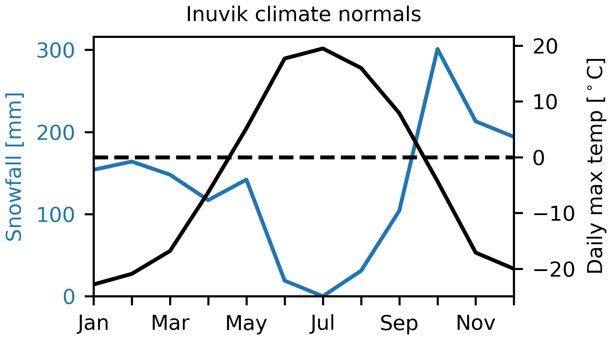
Figure 2 Normal monthly mean snowfall and daily maximum temperature for Inuvik for period of 1985–2010.

2.2 In situ measurements

A number of mid-to-late winter snow transect surveys were compiled (Eppler, 2022) to facilitate method validation which is described in Sect. 4. These are plotted in Fig. 3 and summarized in Table 2, and their positions A–E are labelled in Fig. 1a. These surveys consist of (1) three transects at sites A, B and C that are immediately north of Inuvik, all surveyed by the authors on the same day, (2) one transect, located at site D, provided by Tim Ensom (Wilfred Laurier University) in a fully tree-covered area adjacent to a small creek, and (3) a series of four transect measurements made at the same location, site E, by the Government of Northwest Territories – Department of Environment and Natural Resources (GNWT-ENR) at 2-week intervals at a site with mixed trees and shrubs that is adjacent to the Inuvik Satellite Station Facility. The Tim Ensom transect was surveyed with a 6 cm ESC-30 snow sampler, and all other transects were surveyed with a 6 cm Metric Prairie snow sampler.

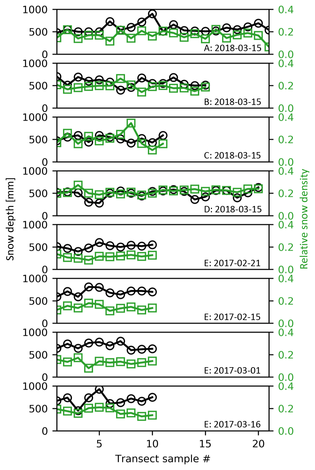
Figure 3 In situ measurements of snow depth and density for the eight transects that are summarized in Table 2.

Table 2 List of transect snow surveys used for in situ comparison with SlopeVar results.

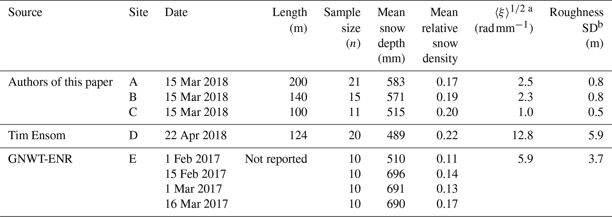
^a Standard deviation of ξ computed over local 500 m × 500 m estimation window. ^b Standard deviation of elevation residuals after removing best-fit planar surface, computed over local 500 m × 500 m estimation window.

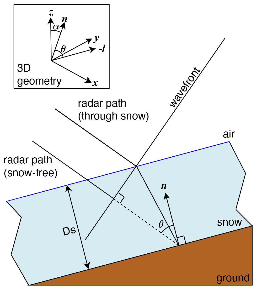
Figure 4 Geometry of refracted ray through a dry-snow layer over an inclined ground surface compared to the unrefracted (straight) ray trajectory. The inset figure shows the general 3D geometry: x, y, and z refer to the local east, north, and vertical directions, and n and l refer to the local slope normal and SAR line-of-sight directions which, together, define the plane depicted in the 2D diagram.

3 Method

3.1 Background

Guneriussen et al. (2001) first described the method of SAR interferometric repeat-pass SWE change estimation, which we summarize as follows. In the case of a dry homogenous layer of snow over ground, a microwave radar signal will penetrate the snow layer, be scattered at the ground surface, and then return through the snow layer. Surface and volume scattering occur at the air–snow interface and within the snowpack, respectively, but for sufficiently dry snow, it can be expected that these contributions will be much less that the primary ground-scattered return (Leinss et al., 2015). The dry-snow layer has a higher real permittivity than air and therefore causes refraction at the air–snow interface, which corresponds to a reduction in the propagation speed of the signal within the snowpack and a corresponding geometric path-length increase. This is shown in Fig. 4, which defines the local 3D geometry and depicts both snow-free and snow-covered cases which diverge at the point where the wavefront reaches the snow surface. The unwrapped phase of the SAR signal due to the dry-snow layer (Φ_s) is given by

$$\begin{array}{}\text{(1)}& {\mathrm{\Phi }}_{\mathrm{s}}\left(\mathit{\theta }\right)={\displaystyle \frac{\mathrm{4}\mathit{\pi }}{\mathit{\lambda }}}{D}_{\mathrm{s}}\left(\sqrt{\mathit{ϵ}\left(\mathit{\rho }\right)-{\sin }^{\mathrm{2}}\mathit{\theta }}-\cos \mathit{\theta }\right),\end{array}$$

and it increases with both snow density ρ (defined dimensionless as the ratio of the gravimetric densities of snow and water) and snow layer thickness D_s (projected along the slope normal direction, represented by direction vector n). Functional dependency on ρ is via the real part of the relative dielectric permittivity ϵ, with other parameters in Eq. (1) being the local incidence angle θ and the radar wavelength λ. Note that θ is defined as the angle between n and −l (reversed SAR line-of-sight direction vector) and therefore depends on both the magnitude and aspect of the local slope. As such, this geometry can be defined everywhere within a SAR scene given maps of spatially varying l, expressed in the local (east, north, vertical) coordinate system and DEM-derived slope magnitude and aspect maps.

In the case of a stratified snowpack, Leinss et al. (2015) have shown that Φ_s is well approximated by a single layer with mean vertical ρ,

$$\begin{array}{}\text{(2)}& \mathit{\rho }\approx {\displaystyle \frac{\mathrm{1}}{Z_{\mathrm{s}}}}\underset{\mathrm{0}}{\overset{Z_{\mathrm{s}}}{\int }}\mathit{\rho }\left(z\right)\mathrm{d}z={\displaystyle \frac{S}{Z_{\mathrm{s}}}},\end{array}$$

where S is the SWE of the snowpack with depth Z_s (measured vertically). Note that $Z_{\mathrm{s}}=D_{\mathrm{s}}/\cos \mathit{\alpha }$, where α is the local topographic slope angle, defined as the angle between n and z. Equations (1) and (2) can be combined to provide the explicit linear relation between dry-snow phase and SWE:

$$\begin{array}{}\text{(3)}& {\mathrm{\Phi }}_{\mathrm{s}}\left(\mathit{\theta }\right)=S{\displaystyle \frac{\mathrm{4}\mathit{\pi }}{\mathit{\lambda }\mathit{\rho }}}\cos \mathit{\alpha }\left(\sqrt{\mathit{ϵ}\left(\mathit{\rho }\right)-{\sin }^{\mathrm{2}}\mathit{\theta }}-\cos \mathit{\theta }\right).\end{array}$$

The relation holds for the general case of repeat-pass interferometric dry-snow phase between any two dry-snow states by replacing total SWE, S, with SWE change, ΔS, and interpreting ρ as the magnitude of the mean ρ of the removed or added snow layer. As such, ΔS can be either positively or negatively valued and ρ ≥ 0.

3.2 Dry-snow phase dependence on local topographic slope

SAR images are formed by focusing complex-valued pulse returns obtained sequentially along a 1D flight track (e.g., satellite orbit segment in the case of spaceborne systems). Each image resolution cell is formed by coherently combining signals received over a finite aperture. Φ_s depends on the local incidence angle, which varies along the aperture. The net effect on the focused image Φ_s, however, is well approximated by considering only the Doppler centroid (i.e., beam center) incident angle at the target (Eppler and Rabus, 2021).

For a focused image, in a local spatial region with constant topographic slope where incidence angle is uniform (gradual across-swath variations can be neglected), a spatially uniform snow layer results in a uniform Φ_s. In contrast, a local spatial region with topographic slope variations will generate Φ_s variations corresponding to variations in the local incidence angle and projection of the snow depth onto the slope normal. The validity of assuming a uniform snow layer under a local window and selecting an appropriate spatial scale are discussed in Sect. 5.2 and 5.5.

Figure 5 depicts the topographic modulation of dry-snow phase explicitly at foreslope, horizontal, and backslope locations. The local incidence angle is less on the foreslope and becomes greater along the transition towards the backslope. The dry-snow phase increases with incidence angle, and therefore this effect causes the phase contribution to increase along the transition from foreslope to backslope.

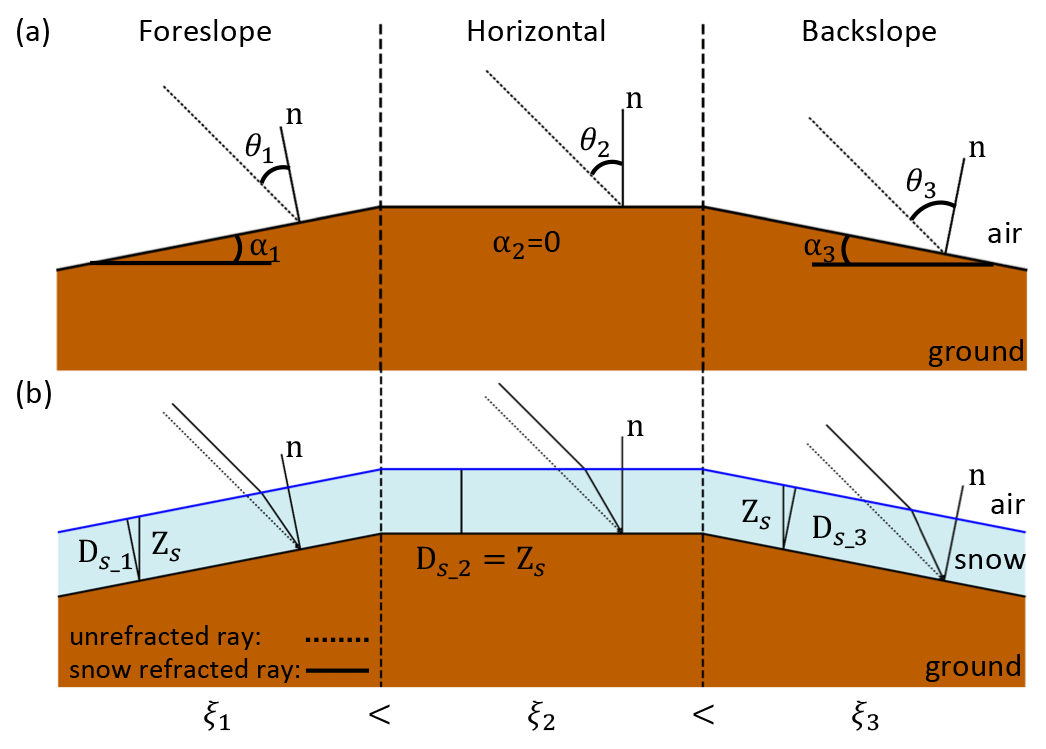
Figure 5 Time evolution of dry-snow refraction geometry for different topographic slopes. Panel (a) depicts a snow-free hill divided into foreslope, horizontal (i.e., hilltop), and backslope with a fixed incident radar direction, and it shows that the local incidence angle increases from foreslope to backslope. Panel (b) depicts the same hill with the addition of a dry-snow layer and shows the corresponding refracted ray geometry. Refraction and corresponding ξ increase from foreslope to backslope. Also illustrated is a reduction in the slope-normal-projected snow depth, D_s, with increasing slope angle, α, while vertical snow depth Z_s is constant. A uniform snow layer is shown which is one of the assumptions of the estimation method described in Sect. 3.3. Note that foreslope and backslope angles (α₁ and α₃) are not assumed to be equal. Also, note that for illustration only, this figure depicts the special case when the SAR line-of-sight and slope normal are coplanar with the vertical direction, but this is generally not the case and is not assumed.

The projection of the snow depth onto the slope normal scales with the cosine of the slope angle and is therefore greatest in horizontal areas and less on both the foreslope and backslope. Considering Eq. (3), if the topographic variation within a SAR scene is known, then the spatially variable Φ_s sensitivity to a uniform SWE layer (ξ) can be computed as

$$\begin{array}{}\text{(4)}& \mathit{\xi }\doteq {\displaystyle \frac{\mathrm{d}{\mathrm{\Phi }}_{\mathrm{s}}}{\mathrm{d}S}}={\displaystyle \frac{\mathrm{4}\mathit{\pi }}{\mathit{\lambda }\mathit{\rho }}}\cos \mathit{\alpha }\left(\sqrt{\mathit{ϵ}\left(\mathit{\rho }\right)-{\sin }^{\mathrm{2}}\mathit{\theta }}-\cos \mathit{\theta }\right),\end{array}$$

where we assume that ρ is known. A spatially varying change in dry SWE during a time interval spanned by two SAR acquisitions will cause a corresponding spatially variable Φ_s, modulated by the topographic sensitivity:

$$\begin{array}{}\text{(5)}& {\mathrm{\Phi }}_{\mathrm{s}}=\mathit{\xi }\mathrm{\Delta }S.\end{array}$$

This effect is depicted in Fig. 6, which shows ξ computed over the RS2-SLA spatial footprint and a late snow-season interferogram which shows spatial phase variations that are correlated with ξ.

Figure 6 (a) Dry-snow phase sensitivity for the RS2-SLA geometry and assuming ρ = 0.3. (b) Topo-corrected 24 d wrapped interferogram 20120317_20120410 showing spatial correlation with ξ in the upland areas (eastern part of image footprint). The rectangular inset area corresponds to the example shown in Fig. 7.

3.3 Estimating absolute ΔSWE by exploiting topographic variation

According to Eq. (5), if Φ_s can be recovered, then the spatially varying SWE change can be directly estimated at the same spatial resolution as the interferogram. However, this requires phase unwrapping which can be difficult for snow-covered interferograms due to both aliasing and local incoherence of the InSAR phase. Furthermore, even if the total unwrapped phase (Φ) can be determined, the phase offset is unknown. One or more reference targets with known SWE change (ΔSWE) are required to estimate the offset. For these reasons, direct estimation of ΔSWE from interferograms is not straightforward. However, we suggest that the effect of topographic modulation of Φ_s, described in Sect. 3.2, allows an absolute estimate without requiring phase unwrapping or knowing the phase offset.

Consider a local estimation window, e.g., 1 km × 1 km. The phase within this window consists of the superposition of Φ_s and other phase components (e.g., due to decorrelation, surface displacement, imperfect topographic correction, soil moisture, or tropospheric delay). For the purposes of estimating ΔSWE, we treat the other phase components as a single error term, Φ_e. Due to the difficulty of phase unwrapping and offset estimation we assume that only the locally de-meaned superposition phase ($\stackrel{\mathrm{̃}}{\mathrm{\Phi }}$) is available:

$$\begin{array}{}\text{(6)}& \stackrel{\mathrm{̃}}{\mathrm{\Phi }}=\mathrm{\Phi }-\langle \mathrm{\Phi }\rangle ={\mathrm{\Phi }}_{\mathrm{s}}-\langle {\mathrm{\Phi }}_{\mathrm{s}}\rangle +{\mathrm{\Phi }}_{\mathrm{e}}-\langle {\mathrm{\Phi }}_{\mathrm{e}}\rangle ,\end{array}$$

where 〈⋅〉 denotes the mean over the window. Initially, for simplicity we assume also that phase variation within the window is limited to a 2π ambiguity interval so that (unwrapped) $\stackrel{\mathrm{̃}}{\mathrm{\Phi }}$ is easily obtained from the corresponding wrapped-phase, ϕ, within the window:

$$\begin{array}{}\text{(7)}& \stackrel{\mathrm{̃}}{\mathrm{\Phi }}=\mathrm{\angle }\left({〈e^{\text{j}\mathit{\varphi }}〉}^{\ast }{e}^{\text{j}\mathit{\varphi }}\right),\end{array}$$

where ^∗ denotes complex conjugation.

The unknown spatially variable SWE change within the window can then be described by

$$\begin{array}{}\text{(8)}& \mathrm{\Delta }S=\langle \mathrm{\Delta }S\rangle +\stackrel{\mathrm{̃}}{\mathrm{\Delta }S},\end{array}$$

where $\stackrel{\mathrm{̃}}{\mathrm{\Delta }S}$ corresponds to the horizontal SWE change variation. ξ can be similarly decomposed as

$$\begin{array}{}\text{(9)}& \mathit{\xi }=\langle \mathit{\xi }\rangle +\stackrel{\mathrm{̃}}{\mathit{\xi }},\end{array}$$

where $\stackrel{\mathrm{̃}}{\mathit{\xi }}$ is the variation in ξ. Substituting Eqs. (8) and (9) into Eq. (5) and expanding yields

$$\begin{array}{}\text{(10)}& {\mathrm{\Phi }}_{\mathrm{s}}=\langle \mathit{\xi }\rangle \langle \mathrm{\Delta }S\rangle +\langle \mathit{\xi }\rangle \stackrel{\mathrm{̃}}{\mathrm{\Delta }S}+\langle \mathrm{\Delta }S\rangle \stackrel{\mathrm{̃}}{\mathit{\xi }}+\stackrel{\mathrm{̃}}{\mathit{\xi }}\stackrel{\mathrm{̃}}{\mathrm{\Delta }S}.\end{array}$$

Substituting Eq. (10) into Eq. (6) and noting that $\langle \stackrel{\mathrm{̃}}{\mathrm{\Delta }S}\rangle =\langle \stackrel{\mathrm{̃}}{\mathit{\xi }}\rangle =\mathrm{0}$ gives

$$\begin{array}{}\text{(11)}& \stackrel{\mathrm{̃}}{\mathrm{\Phi }}=\langle \mathrm{\Delta }S\rangle \stackrel{\mathrm{̃}}{\mathit{\xi }}+\langle \mathit{\xi }\rangle \stackrel{\mathrm{̃}}{\mathrm{\Delta }S}+\stackrel{\mathrm{̃}}{\mathit{\xi }}\stackrel{\mathrm{̃}}{\mathrm{\Delta }S}-〈\stackrel{\mathrm{̃}}{\mathit{\xi }}\stackrel{\mathrm{̃}}{\mathrm{\Delta }S}〉+{\mathrm{\Phi }}_{\mathrm{e}}-〈{\mathrm{\Phi }}_{\mathrm{e}}〉.\end{array}$$

Assuming $\stackrel{\mathrm{̃}}{\mathrm{\Phi }}$ correlates with $\stackrel{\mathrm{̃}}{\mathit{\xi }}$ with the proportionality 〈ΔS〉, we introduce the following correlation-based estimator for 〈ΔS〉:

$$\begin{array}{}\text{(12)}& \widehat{\mathrm{\Delta }S}:={\displaystyle \frac{〈\stackrel{\mathrm{̃}}{\mathit{\xi }}\stackrel{\mathrm{̃}}{\mathrm{\Phi }}〉}{〈{\stackrel{\mathrm{̃}}{\mathit{\xi }}}^{\mathrm{2}}〉}}=\langle \mathrm{\Delta }S\rangle +{\displaystyle \frac{\mathrm{1}}{〈{\stackrel{\mathrm{̃}}{\mathit{\xi }}}^{\mathrm{2}}〉}}\left[\langle \mathit{\xi }\rangle 〈\stackrel{\mathrm{̃}}{\mathit{\xi }}\stackrel{\mathrm{̃}}{\mathrm{\Delta }S}〉+〈{\stackrel{\mathrm{̃}}{\mathit{\xi }}}^{\mathrm{2}}\stackrel{\mathrm{̃}}{\mathrm{\Delta }S}〉+〈\stackrel{\mathrm{̃}}{\mathit{\xi }}{\mathrm{\Phi }}_{\mathrm{e}}〉\right].\end{array}$$

This estimator correlates $\stackrel{\mathrm{̃}}{\mathrm{\Phi }}$ with $\stackrel{\mathrm{̃}}{\mathit{\xi }}$ and relies on the assumption that the horizontal SWE change distribution is uniform within the window and that Φ_e components are uncorrelated with $\stackrel{\mathrm{̃}}{\mathit{\xi }}$. The bias of $\widehat{\mathrm{\Delta }S}$ with respect to 〈ΔS〉 is given by

$$\begin{array}{}\text{(13)}& \begin{array}{rl}& E\left(\widehat{\mathrm{\Delta }S}\right)-\langle \mathrm{\Delta }S\rangle \\ & ={\displaystyle \frac{\mathrm{1}}{〈{\stackrel{\mathrm{̃}}{\mathit{\xi }}}^{\mathrm{2}}〉}}\left[\langle \mathit{\xi }\rangle E\left(〈\stackrel{\mathrm{̃}}{\mathit{\xi }}\stackrel{\mathrm{̃}}{\mathrm{\Delta }S}〉\right)+E\left(〈{\stackrel{\mathrm{̃}}{\mathit{\xi }}}^{\mathrm{2}}\stackrel{\mathrm{̃}}{\mathrm{\Delta }S}〉\right)+E\left(〈\stackrel{\mathrm{̃}}{\mathit{\xi }}{\mathrm{\Phi }}_{\mathrm{e}}〉\right)\right],\end{array}\end{array}$$

where E(⋅) denotes the expectation. Therefore, $\widehat{\mathrm{\Delta }S}$ is biased by the components of $\stackrel{\mathrm{̃}}{\mathrm{\Delta }S}$ that are systematically correlated with either $\stackrel{\mathrm{̃}}{\mathit{\xi }}$ or ${\stackrel{\mathrm{̃}}{\mathit{\xi }}}^{\mathrm{2}}$, as well as by Φ_e components systematically correlated with $\stackrel{\mathrm{̃}}{\mathit{\xi }}$. The significance of the different bias terms is examined in Sects. 5.2 and 5.3.

3.4 Wrapped-phase (“SlopeVar”) estimator

The estimator defined in Eq. (12) requires $\stackrel{\mathrm{̃}}{\mathrm{\Phi }}$ within the spatial window of consideration, and we have assumed so far that this can be obtained from ϕ through Eq. (7) implicitly assuming phase variations in the window are limited to a maximum of 2π. As shown by Just and Bamler (1994), decorrelation to any degree results in a per-target phase distribution that is not bound by the ±π interval, and so this condition is never strictly met. Except for high-coherence areas with limited short-scale phase variation, either the phase within the window must be unwrapped or an alternative wrapped-phase version of the estimator is required.

Here we propose such an alternative estimator (which we denote the “SlopeVar” estimator) that uses periodogram optimization to iteratively estimate 〈ΔS〉 using the set of wrapped phase ϕ under the window

$$\begin{array}{}\text{(14)}& {\widehat{\mathrm{\Delta }S}}_{\mathrm{w}}=\underset{\mathrm{\Delta }{S}_{\mathrm{w}}}{\text{argmax}}\left|〈e^{j\left(\mathit{\varphi }-\mathrm{\Delta }{S}_{\mathrm{w}}\stackrel{\mathrm{̃}}{\mathit{\xi }}\right)}〉\right|.\end{array}$$

Considering Eq. (11) and the fact that e^jϕ=e^jΦ, Eq. (14) can be expanded to show the components of ϕ,

$$\begin{array}{}\text{(15)}& \begin{array}{rl}{\widehat{\mathrm{\Delta }S}}_{\mathrm{w}}& =\underset{\mathrm{\Delta }{S}_{\mathrm{w}}}{\text{argmax}}\\ & \left|〈e^{j\left(\langle \mathrm{\Delta }S\rangle \stackrel{\mathrm{̃}}{\mathit{\xi }}+\langle \mathit{\xi }\rangle \stackrel{\mathrm{̃}}{\mathrm{\Delta }S}+\stackrel{\mathrm{̃}}{\mathit{\xi }}\stackrel{\mathrm{̃}}{\mathrm{\Delta }S}-〈\stackrel{\mathrm{̃}}{\mathit{\xi }}\stackrel{\mathrm{̃}}{\mathrm{\Delta }S}〉+{\mathrm{\Phi }}_{\mathrm{e}}-\mathrm{\Delta }{S}_{\mathrm{w}}\stackrel{\mathrm{̃}}{\mathit{\xi }}\right)}〉\right|.\end{array}\end{array}$$

In the case where Φ_e=0 and $\stackrel{\mathrm{̃}}{\mathrm{\Delta }S}=\mathrm{0}$, this yields an unbiased estimate, i.e., ${\widehat{\mathrm{\Delta }S}}_{\mathrm{w}}=\langle \mathrm{\Delta }S\rangle$, otherwise the $\langle \mathit{\xi }\rangle \stackrel{\mathrm{̃}}{\mathrm{\Delta }S}$, $\stackrel{\mathrm{̃}}{\mathit{\xi }}\stackrel{\mathrm{̃}}{\mathrm{\Delta }S}$, and $〈\stackrel{\mathrm{̃}}{\mathit{\xi }}\stackrel{\mathrm{̃}}{\mathrm{\Delta }S}〉$ terms in Eq. (15) will bias ${\widehat{\mathrm{\Delta }S}}_{\mathrm{w}}$.

Figure 7 shows an example of the SlopeVar estimator being applied to a 1 km×1 km (ground range × azimuth) window for the inset area labelled in Fig. 6. $\stackrel{\mathrm{̃}}{\mathrm{\Phi }}$ is moderately correlated with $\stackrel{\mathrm{̃}}{\mathit{\xi }}$ over the window as seen by comparing Fig. 7a and b and by examining the 2D histogram in Fig. 7d. Figure 7e shows the periodogram with a distinct peak at ΔSWE of 28 mm. Figure 7c shows the effect of removing the Φ_s component assuming constant ΔSWE of 28 mm under the window, which results in a much more uniform phase, although residual variations can still be seen.

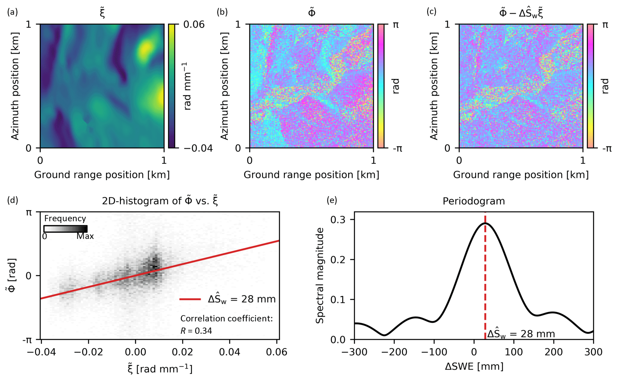
Figure 7 Example of SlopeVar ΔSWE estimation over a 1 km × 1 km window corresponding to the inset area shown in Fig. 6 for the 20120317_20120410 interferogram. (a) Variation in dry-snow phase sensitivity, (b) demeaned phase, (c) ΔSWE-corrected demeaned phase (using SlopeVar estimate, ${\widehat{\mathrm{\Delta }S}}_{\text{w}}$), (d) 2D histogram of demeaned phase vs. variation in dry-snow phase sensitivity with line corresponding to ${\widehat{\mathrm{\Delta }S}}_{\text{w}}$, and (e) periodogram with peak corresponding to ${\widehat{\mathrm{\Delta }S}}_{\text{w}}$.

3.5 Estimator implementation

The estimator was implemented as a Python software module (Eppler, 2022). Input interferograms were generated by co-registering the set of RS2-SLA SLCs to a common master SLC and computing sequential topographic phase-corrected 3 × 12 (range pixels × azimuth pixels) multi-looked interferograms using the GAMMA software package (GAMMA Remote Sensing AG, Switzerland). Multi-looking was performed to better match the sample spacing of the interferograms to that of the DEM-derived ξ map. This improved estimator computation runtime and was seen to have a negligible effect on the resulting ΔSWE estimates. All interferograms were visually inspected, and those with sparse coherence, typically those spanning the spring melt and early winter periods, were discarded from further analysis.

For simplicity, we only processed sequential interferograms since these provide the best coherence during the dry-snow season. However, for distributed scatterers which predominate in natural terrain, additional interferograms (e.g., 48, 72 d, …) are known to allow for a reduction in the variance in estimated sequential phases using a phase-linking estimator (e.g., Guarnieri and Tebaldini, 2008). This is because such scatterers exhibit complex Gaussian scattering statistics which are not fully characterized by the set of sequential interferograms alone.

We found the estimator to be sensitive to errors in ξ, especially those resulting from DEM errors and interpolation errors. High-spatial-frequency errors in the ξ map tend to bias the estimated ΔSWE magnitude towards zero (discussed in Sect. 5.4). We initially used the raw TanDEM-X DEM, which we cubic-resampled to the multi-looked SAR geometry, to compute the slope and aspect angle maps required to compute ξ. The resulting ξ map contained high-frequency artifacts from the cubic interpolation, as well as substantial errors due to stitching artifacts in the raw DEM. We did not thoroughly investigate the issue of the most appropriate interpolator, and so it may be possible to reduce these errors by using a different interpolator. Estimator performance improved significantly after we (1) manually identified and masked local DEM stitching artifacts and interpolated over them, (2) smoothed the DEM using a 2D Gaussian filter with a standard deviation of three DEM pixels (resulting in approximately 90 m spatial resolution) to reduce high-frequency DEM errors, and (3) computed the slope angle maps prior to resampling to the SAR geometry. Note that to compute ξ according to Eq. (4), we computed ϵ of dry snow as $\mathit{ϵ}\left(\mathit{\rho }\right)=\mathrm{1}+\mathrm{1.5995}\mathit{\rho }+\mathrm{1.861}{\mathit{\rho }}^{\mathrm{3}}$, according to Mätzler (1987), and for simplicity assumed ρ=0.3 for all estimates (discussed further in Sect. 5.1).

We then implemented the SlopeVar estimator described in Sect. 3.4. For each candidate value of ΔS_w, the periodogram magnitude, $\mathrm{|}\langle e^{j(\mathit{\varphi }-\mathrm{\Delta }{S}_{\mathrm{w}}\stackrel{\mathrm{̃}}{\mathit{\xi }})}\rangle \mathrm{|}$, can be computed efficiently using a 2D fast-Fourier-transform-based rectangular smooth filter over the complex-valued interferogram, allowing for the generation of spatially oversampled maps at the interferogram sample spacing instead of the much coarser estimation window size. We evaluated the periodogram over the ΔSWE range of [−50 mm, 80 mm] with an interval spacing of 2 mm. Peak locations for each spatial point were then refined by fitting a quadratic by least squares using three points centered on the maximum value found over the search grid.

Solutions where the maximum was within two grid intervals from the edge of the search range were labelled as invalid. This provides a means for excluding poor results from low-coherence areas since for these areas the periodogram analysis typically does not result in a peak within the search range. We considered adding an additional exclusion threshold based on coherence magnitude but found it unnecessary. Water-body areas were also labelled as invalid.

Figure 8a shows the resulting ΔSWE map after applying the estimator to all areas of the example interferogram depicted in Fig. 6 using a 500 m square estimation window.

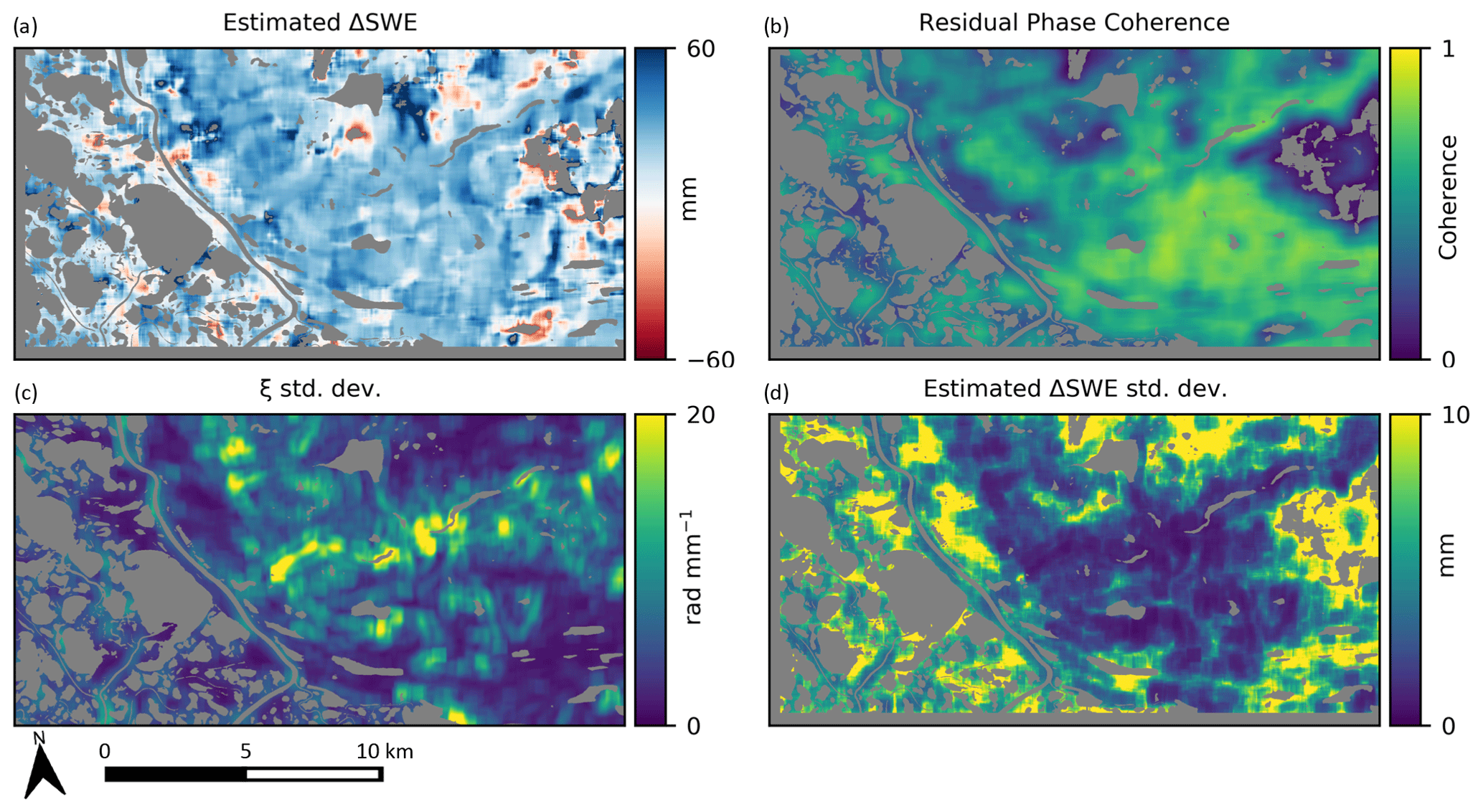
Figure 8 Example of estimated ΔSWE and ΔSWE standard deviation due to uncorrelated phase components (described in Sect. 3.6) for the 20120317_20120410 scene pair (same interferogram as shown in Figs. 6 and 7) using a window size of 500 m × 500 m. (a) Estimated ΔSWE using the SlopeVar estimator, (b) coherence of residual phase after estimated dry-snow phase correction, (c) standard deviation of ξ computed over the estimation window, and (d) Monte-Carlo-estimated standard deviation of estimated ΔSWE generated with ensemble of 40 simulated interferograms. Water areas are greyed out in each panel. Points with no solution in the ΔSWE search range are also greyed out in panels (a), (b), and (c).

3.6 Monte Carlo estimation of ΔSWE estimation variance

The amount of decorrelation can vary significantly both spatially within each interferogram and temporally depending on changing surface conditions and pass-to-pass variations in the SAR orbit. It is therefore important to estimate the ΔSWE variance contribution as a space- and time-varying quantity.

Specifying the transfer function between phase noise and ${\widehat{\mathrm{\Delta }S}}_{\mathrm{w}}$ variance is made difficult by the fact that the distribution of $\stackrel{\mathrm{̃}}{\mathit{\xi }}$ is generally unique for each estimation window. We decided to apply the Monte Carlo approach by simulating a sufficiently large ensemble of zero-signal partially decorrelated interferograms, applying the ΔSWE estimation on each instance, and then computing statistics over the ensemble of estimates. We approximate the phase noise as a circular complex stationary white process with zero mean phase as described by Just and Bamler (1994) and which is uniquely specified by the coherence magnitude, γ. We estimate γ as the ensemble coherence of the residual phase after removing Φ_s estimated using ${\widehat{\mathrm{\Delta }S}}_{\mathrm{w}}$:

$$\begin{array}{}\text{(16)}& \widehat{\mathit{\gamma }}=\left|〈e^{j\left(\mathit{\varphi }-\widehat{\mathrm{\Delta }{S}_{\mathrm{w}}}\stackrel{\mathrm{̃}}{\mathit{\xi }}\right)}〉\right|.\end{array}$$

Figure 8b–d, respectively, show the residual phase coherence map, the standard deviation of ξ under the window (i.e., $\langle {\stackrel{\mathrm{̃}}{\mathit{\xi }}}^{\mathrm{2}}{\rangle }^{\mathrm{1}/\mathrm{2}})$, and the resulting Monte-Carlo-based error estimation for the same interferogram depicted in Fig. 6. Local factors affecting the ${\widehat{\mathrm{\Delta }S}}_{\mathrm{w}}$ variance include (1) the residual coherence magnitude, (2) the diversity of ξ within the estimation window, and (3) the spatial support under the window (areas adjacent to water bodies have a smaller ensemble of valid phase samples and hence a larger variance).

3.7 Precision comparison with Delta-K ΔSWE estimator

Our method has some similarity with the Delta-K method for estimating ΔSWE in that both methods exploit a diversity in the dry-snow phase sensitivity so that absolute ΔSWE can be estimated without the need for phase unwrapping. Furthermore, both methods operate over an estimation window, yielding results at a resolution lower than the single-look resolution. In order to compare the two methods, we consider their relative precision estimated over a spatial window with N multi-looked-resolution cells and assume Gaussian phase noise, which is reasonable when multi-looked interferograms with sufficient looks are used (i.e., > 10 as noted by Hagberg et al., 1995). Note that for the Delta-K method, multi-looking of sub-band interferograms prior to computing the band difference phases has been suggested by Bamler and Eineder (2005) to preserve the Gaussian phase noise assumption and shown by De Zan et al. (2015) to yield better precision than the alternative of first computing the sub-band difference and then multi-looking.

The Delta-K method exploits the ξ diversity that exists between separate radar-frequency sub-bands corresponding to $\mathit{\xi }\pm \mathrm{\Delta }\mathit{\xi }/\mathrm{2}$, where ξ in this case is the value at the central carrier frequency, and $\mathrm{\Delta }\mathit{\xi }=B(\mathrm{1}-b)\mathit{\xi }$, where $B\in [\mathrm{0},\mathrm{1}]$ is the bandwidth of the SAR normalized with respect to carrier frequency and $b\in [\mathrm{0},\mathrm{1}]$ is the sub-bandwidth fraction used. Assuming multi-looked phase noise with variance ${\mathit{\sigma }}_{\mathrm{\Phi }}^{\mathrm{2}}$, the mean sub-band interferometric phase will have the variance ${\mathit{\sigma }}_{\mathrm{\Phi }}^{\mathrm{2}}/bN$, and therefore the Delta-K difference phase will have the variance ${\mathit{\sigma }}_{\mathrm{\Phi }\mathit{\_}DK}^{\mathrm{2}}=\mathrm{2}{\mathit{\sigma }}_{\mathrm{\Phi }}^{\mathrm{2}}/bN$. Delta-K estimates ΔSWE according to ${\widehat{\mathrm{\Delta }S}}_{\text{DK}}={\mathrm{\Phi }}_{\text{DK}}/\mathrm{\Delta }\mathit{\xi }$, and therefore the ${\widehat{\mathrm{\Delta }S}}_{\text{DK}}$ standard deviation (σ_{ΔS_DK}) is

$$\begin{array}{}\text{(17)}& {\mathit{\sigma }}_{\mathrm{\Delta }S\mathit{\_}\text{DK}}=\sqrt{{\displaystyle \frac{\mathrm{2}}{N}}}{\displaystyle \frac{{\mathit{\sigma }}_{\mathrm{\Phi }}}{B(\mathrm{1}-b)b^{\frac{\mathrm{1}}{\mathrm{2}}}\mathit{\xi }}}.\end{array}$$

For the SlopeVar method, the estimation of ΔSWE corresponds to a linear regression over N samples, and therefore, assuming $\stackrel{\mathrm{̃}}{\mathit{\xi }}$ is Gaussian-distributed under the estimation window with variance $\langle {\stackrel{\mathrm{̃}}{\mathit{\xi }}}^{\mathrm{2}}\rangle$, the estimation standard deviation (σ_{ΔS_SV}) is

$$\begin{array}{}\text{(18)}& {\mathit{\sigma }}_{\mathrm{\Delta }S\mathit{\_}\text{SV}}={\displaystyle \frac{{\mathit{\sigma }}_{\mathrm{\Phi }}}{\sqrt{N}{〈{\stackrel{\mathrm{̃}}{\mathit{\xi }}}^{\mathrm{2}}〉}^{\mathrm{1}/\mathrm{2}}}}.\end{array}$$

The relative estimation precision ratio between the two methods is therefore given by

$$\begin{array}{}\text{(19)}& {\displaystyle \frac{{\mathit{\sigma }}_{\mathrm{\Delta }S\mathit{\_}\text{DK}}}{{\mathit{\sigma }}_{\mathrm{\Delta }S\mathit{\_}\text{SV}}}}={\displaystyle \frac{\sqrt{\mathrm{2}}{〈{\stackrel{\mathrm{̃}}{\mathit{\xi }}}^{\mathrm{2}}〉}^{\frac{\mathrm{1}}{\mathrm{2}}}}{B(\mathrm{1}-b)b^{\frac{\mathrm{1}}{\mathrm{2}}}\langle \mathit{\xi }\rangle }},\end{array}$$

where we have replaced ξ in Eq. (17) with the mean under the estimation window, 〈ξ〉. We use $b=\mathrm{1}/\mathrm{3}$, which, neglecting system noise, is the optimum value for minimizing σ_{ΔS_DK}, and B=0.0185, which is the normalized range bandwidth for the RADARSAT-2 Spotlight-A mode. Figure 9 shows the distribution of ${\mathit{\sigma }}_{\mathrm{\Delta }S\mathit{\_}\text{DK}}/{\mathit{\sigma }}_{\mathrm{\Delta }S\mathit{\_}\text{SV}}$ computed for all 500 m square estimation windows in the RS2-SLA study footprint, excluding water bodies. The distribution has a median value of 3.8 and is > 1 for 97.5 % of the area, indicating that the SlopeVar estimator can be expected to provide substantially better ΔSWE precision compared to Delta-K for the great majority of areas within the study footprint.

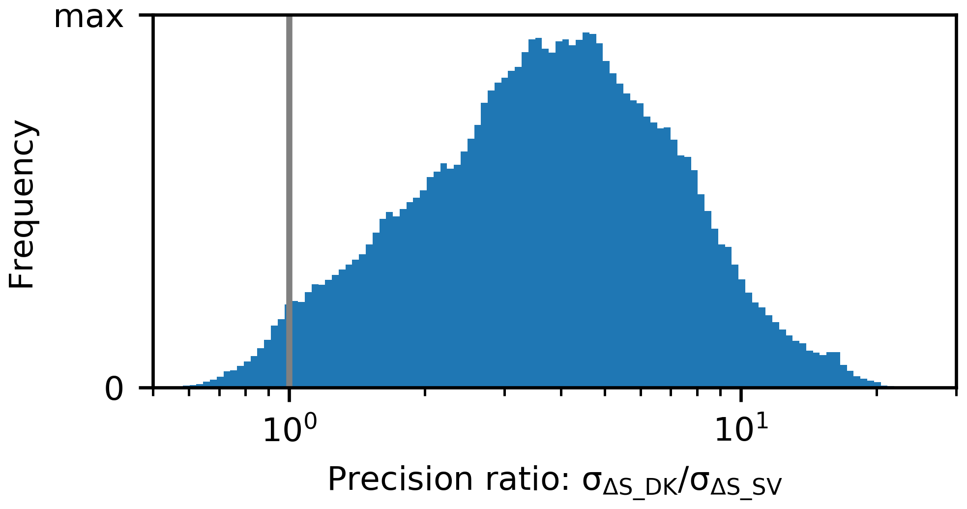
Figure 9 Histogram of the predicted ΔSWE estimation precision ratio between the Delta-K and SlopeVar methods (${\mathit{\sigma }}_{\mathrm{\Delta }S\mathit{\_}\text{DK}}/{\mathit{\sigma }}_{\mathrm{\Delta }S\mathit{\_}\text{SV}}$) for all 500 m square estimation windows in the RS2-SLA study footprint. The vertical bar denotes the point of equal precision (i.e., ${\mathit{\sigma }}_{\mathrm{\Delta }S\mathit{\_}\text{DK}}/{\mathit{\sigma }}_{\mathrm{\Delta }S\mathit{\_}\text{SV}}$ = 1). This shows that the SlopeVar estimator provides substantially better precision for almost all areas within the study footprint.

4 Results

4.1 ΔSWE estimation maps

We computed 95 coherent sequential interferograms from the assembled set of 120 RS2-SLA SLCs, and these were used with the SlopeVar estimator to generate ${\widehat{\mathrm{\Delta }S}}_{\mathrm{w}}$ maps using an estimation window of 500 m × 500 m (ground range × azimuth). This corresponds to 46 snow-season interferograms over two partial and eight complete snow seasons and 49 non-snow interferograms over nine snow-free seasons. The estimator was run on the snow-free-season interferograms to serve as control cases since these are known to have zero dry-snow ΔSWE. Additionally, the Monte-Carlo-based variance estimator described in Sect. 3.6 was run on all interferograms. Water bodies and areas with no valid solution from the periodogram peak-finding analysis were labelled as invalid and masked out. Figure 10 shows an example set of five such ΔSWE maps from the 2017–2018 snow season (all snow-season ΔSWE maps from the 2012–2021 dataset are shown in Fig. S1 in the Supplement).

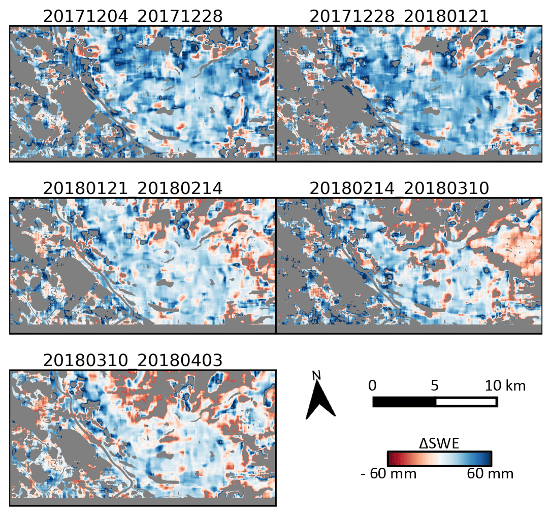
Figure 10 Dry-snow-season ΔSWE maps from the 2017–2018 snow season, estimated with the SlopeVar estimator. Water areas and points with no solution in the ΔSWE search range are greyed out. Date pairs are formatted as yyyymmdd_yyyymmdd.

4.2 Comparison of ΔSWE estimates with in situ measurements

To compare the results with the in situ transect measurements presented in Sect. 2.2, we generated snow-season cumulative SWE maps by integrating the sequential ${\widehat{\mathrm{\Delta }S}}_{\mathrm{w}}$ maps through time, starting with the first dry-snow interferogram identified for each snow season. As discussed in Sect. 3.5, some ${\widehat{\mathrm{\Delta }S}}_{\mathrm{w}}$ values are labelled as invalid due to a lack of a distinct periodogram peak. On average these correspond to about 10 % of non-water spatial samples, and therefore, in order to preserve temporal continuity for the integration, these were replaced with values obtained by smoothing all valid estimates within a 2 km square window. The cumulative SWE maps do not represent estimates of true absolute SWE because early snow-season interferograms are generally not sufficiently coherent to allow ΔSWE estimation, and therefore some amount of accumulated SWE is not accounted for. Therefore, for the comparison, the in situ measurements correspond to an upper limit for the expected SlopeVar-estimated total SWE maps, neglecting any biases. However, given the error sources described in Sect. 5, actual estimates may exceed this expected upper limit.

We also estimated variances for the cumulative SWE maps by summing the Monte-Carlo-derived per-interval variance estimates, assuming they are uncorrelated through time.

For each transect dataset, all SWE measurements were averaged to generate a mean value for the local area and the sample standard deviation was used to compute a corresponding standard error. This was done because the transect lengths, listed in Table 2, were 200 m or less, being well within the 500 m SlopeVar estimator window size. The in situ measurements were each made on a particular date, whereas the InSAR cumulative SWE maps are produced at 24 d intervals. The cumulative SWE maps temporally bracketing each transect date were therefore sampled at the spatial mean position of the transect and then linearly interpolated in time to generate a cumulative SWE estimate for that point in space and time. Likewise, the error variance maps were also interpolated and converted to standard deviations.

Figure 11 shows a scatterplot comparison of the InSAR-derived cumulative SWE estimates and the transect mean SWE values. Vertical and horizontal error bars correspond to 1 standard deviation and 1 standard error, respectively. Seven of the eight transects are within 1 standard deviation of the 1:1 line and demonstrate good agreement between the measured and estimated values. Treating the transect mean values as truth and neglecting the unaccounted early snow-season SWE, the RMSE for all transect comparisons is 14.8 mm and the bias is −6.6 mm. It is noteworthy that the author-surveyed transects (locations “A”, “B”, and “C”) correspond to areas of low topographic variation as indicated by the two rightmost columns of Table 2, and, as shown in Fig. 11, locations “A” and “C” have larger predicted total SWE standard deviations (i.e., > 25 mm). This is consistent with the fact that estimation variance is expected to increase with decreasing ξ diversity.

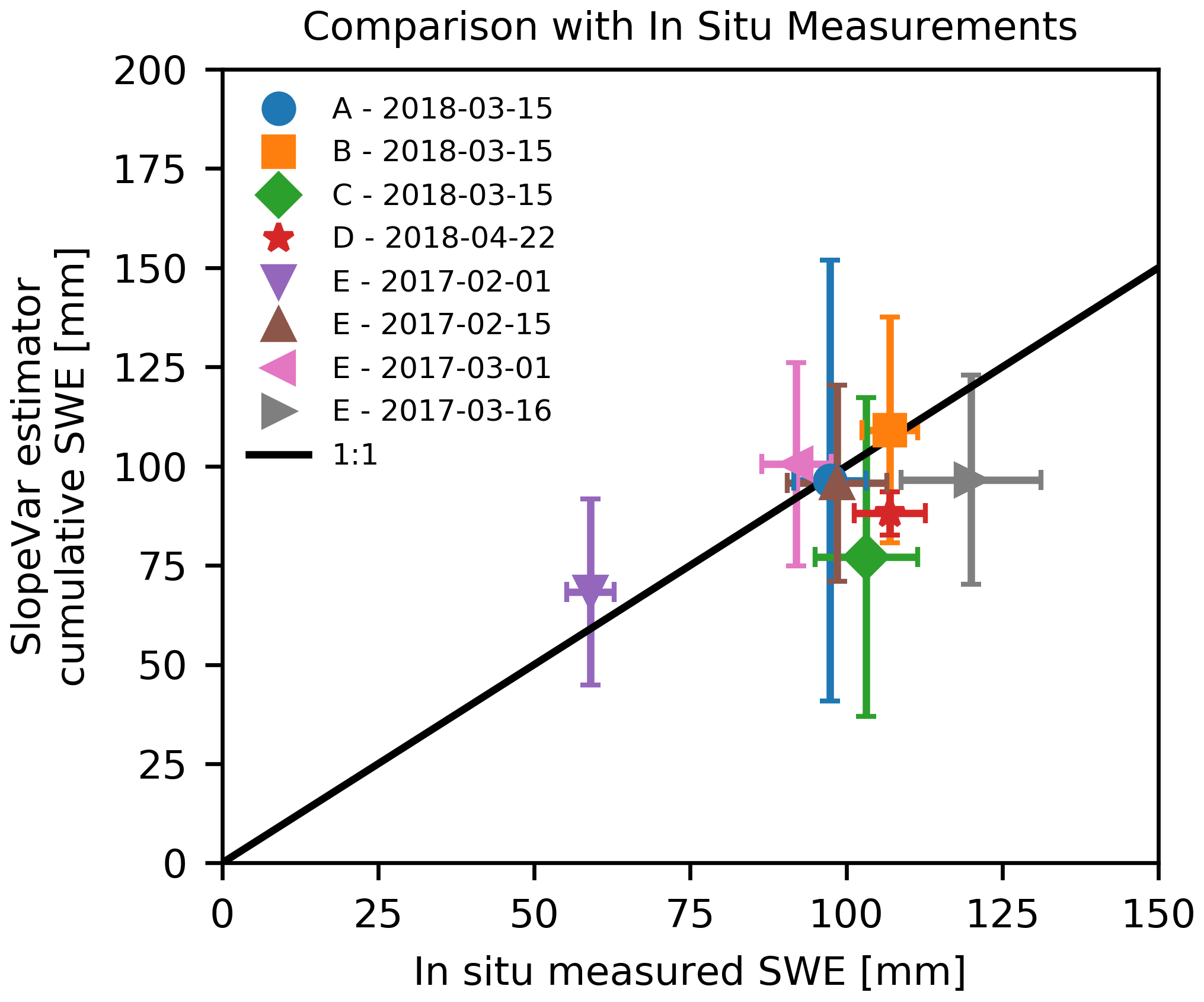
Figure 11 Comparison of SlopeVar estimator cumulative SWE with in situ snow-tube-sampled SWE transect measurements. Error bars correspond to the snow-season accumulated SWE standard deviation (vertical) and the transect measurement standard error (horizontal). Labels A–E correspond to the survey locations, shown in Fig. 1a.

4.3 Comparison of ΔSWE estimates with predicted temporal change

The estimator results were examined temporally by comparing the spatial mean of each ${\widehat{\mathrm{\Delta }S}}_{\mathrm{w}}$ map, after projection to ground-range geometry, with the corresponding SWE change predicted by the European Centre for Medium-Range Weather Forecasts (ECMWF) ERA5 reanalysis model (Hersbach et al., 2020) over the same time interval. We chose ERA5 for comparison based on Mortimer et al. (2020), who report that it compares favourably with independent snow course data and more so than currently available global passive microwave products do. The gridded ERA5 results were spatially interpolated to the RS2-SLA scene center. Note that all but five of the analyzed interferograms span 24 d intervals. The additional five intervals each span 48 d due to missed SAR acquisitions. For the temporal comparison, each of these five intervals were split into two 24 d intervals with half the ${\widehat{\mathrm{\Delta }S}}_{\mathrm{w}}$ arbitrarily assigned to each interval.

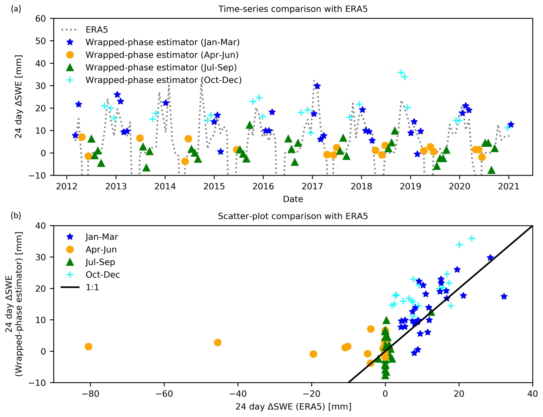
Figure 12 Time series (a) and scatterplot (b) comparisons of SlopeVar estimator 24 d interval ΔSWE with ERA5 reanalysis estimates. SlopeVar estimator point symbols are separated according to season to illustrate the seasonal dependence of the bias (especially the difference between October–December and January–March points) apparent in the scatterplot.

Figure 12a compares the continuous ERA5 24 d interval ΔSWE history time series with the SlopeVar estimator results. Figure 12b shows the same data as a scatterplot comparison. Both plots are labelled according to the time of year as four annual quarters to highlight seasonal effects. Treating the ERA5 estimates as truth, Table 3 shows error statistics (bias, RMSE, and correlation coefficient) for a number of temporal subsets that include the four seasonal quarters, all intervals, the nominal dry-snow period (October–March), and the “no snow” intervals (all intervals with zero ERA5 SWE at both interval endpoints).

Table 3 SWE error statistics for SlopeVar estimator compared to ERA5 reanalysis estimates.

^∗ All intervals with zero ERA5 SWE at both interval endpoints.

Regarding correspondence with ERA5, we are primarily concerned with the October–December and January–March estimates because these correspond to the dry-snow period when the estimator is expected to provide useful results. Figure 12b shows that these do follow the 1:1 correspondence line. However, the October–December points appear to have a significant positive bias, whereas the January–March points do not. This is quantified in Table 3, which shows that, in aggregate, the October–March time period has a correlation of 0.57 with respect to ERA5, which is moderately strong. There is an 8.6 mm per-interval ΔSWE bias for October–December but only 1.7 mm for January–March. This is consistent with the expected impact of early freeze-season heave, which is discussed further in Sect. 5.3.2. The no-snow intervals are of interest because they serve as a control set with known zero ΔSWE. These show a bias of +1.7 mm, which is discussed further in Sect. 5.3.2. The RMSE of the no-snow set is 4.2 mm, which serves as a measure of the estimation uncertainty due to factors other than ΔSWE inhomogeneity. The April–June intervals are included for completeness even though these are not expected to agree because this corresponds to the snowmelt period. This is especially apparent for the two intervals with large negative ERA5 ΔSWE values corresponding to periods of intense snowmelt. The SlopeVar estimates for these periods are near zero likely because only snow-free areas (snow already melted) are coherent and hence contribute to the estimates, and seasonal active-layer thaw has not yet commenced.

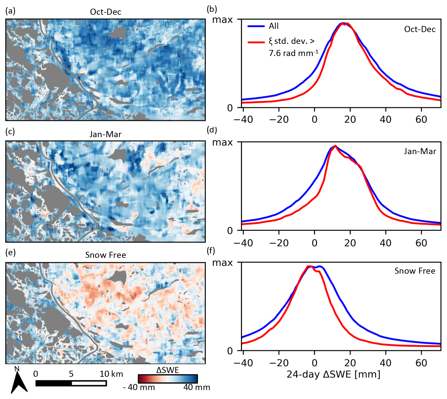
Figure 13 (a), (c), and (e) Comparison of mean seasonal ΔSWE maps, showing means for the early snow season (October–December), late snow season (January–March), and all snow-free periods (temporal subsets described in Table 3). Water areas are greyed out. (b), (d), and (f) Corresponding normalized seasonal distributions of all valid ΔSWE estimates. Distributions for the subset of estimates for high ξ diversity areas are also shown.

4.4 Distribution of the estimated ΔSWE

Spatial variations in the ${\widehat{\mathrm{\Delta }S}}_{\mathrm{w}}$ maps are due to a combination of true ΔSWE spatial variations, stochastic error due to decorrelation, and spatially variable biases as described in Sect. 5. An independent set of densely sampled ΔSWE measurements over our study area does not exist, which precludes direct estimation of the errors. Instead, we compare temporally averaged seasonal subsets of the ${\widehat{\mathrm{\Delta }S}}_{\mathrm{w}}$ maps since we expect the bias to differ between seasons. Figure 13a, c, and e show the temporal mean ΔSWE maps for the early snow season (October–December), late snow season (January–March), and all snow-free intervals. These show a moderate degree of negative correlation between the October–December and snow-free maps, especially in the upland area east of the delta margin. The Pearson correlation coefficients between the three maps are R_{October–December/January–March} = 0.28; R_{October–December/Snow-free} = −0.52; and R_{January–March/Snow-free} = −0.17. These are consistent with a dominant bias contribution from surface normal heave and subsidence contributing to the October–December and snow-free subsets but with opposite polarity. The weaker correlations between these and the January–March subset suggest a weaker surface-normal bias contribution during this period which is consistent with the expected annual cycle of active-layer heave and subsidence discussed further in Sect. 5.3.2.

Figure 13b, d, and f show the normalized distributions for all ΔSWE estimates partitioned by season. Since the snow-free intervals have a known ΔSWE of zero, a global RMSE value can be computed. This value, computed over all non-water areas and all snow-free maps, is RMSE_snow-free = 21 mm. We know from Eqs. (13) and (30) that both additive and multiplicative bias contributions are modulated by the local ξ variance inverse. We repeated the RMSE calculation for the top ξ variance quartile of spatial samples (corresponding to threshold of $\langle {\stackrel{\mathrm{̃}}{\mathit{\xi }}}^{\mathrm{2}}{\rangle }^{\mathrm{1}/\mathrm{2}}$ > 7.6 rad mm⁻¹), resulting in RMSE_snow-free = 15 mm, which shows that the impact of bias can be reduced by restricting the estimator to areas with greater ξ diversity, albeit with a loss of spatial coverage. Normalized distributions for this restricted subset are also shown in Fig. 13b, d, and f.

5 Discussion

5.1 Snow density misspecification

Our proposed method relies on knowing ξ, which, as shown in Eq. (3), depends on ρ. Therefore ρ must either be known a priori or an assumed value must be specified. Here we assess the effect of misspecifying ρ. Since the method estimates ΔSWE from the interferometric phase, the required ρ corresponds to the snowpack change rather than the actual bulk ρ of the snowpack. For the case of fresh snowfall on a dense late season snowpack, the ρ of the added layer will be less than the mean ρ before and after the change.

A misspecification of ρ will bias the resulting ΔSWE estimate. This effect can be quantified by parameterizing ξ with respect to ρ so that Φ_s(ρ)=ξ(ρ)ΔS. The fractional ΔSWE bias caused by specifying ρ^′ rather than the true value, ρ, is

$$\begin{array}{}\text{(20)}& {\displaystyle \frac{\widehat{\mathrm{\Delta }S}-\mathrm{\Delta }S}{\mathrm{\Delta }S}}={\displaystyle \frac{\mathit{\xi }\left(\mathit{\rho }\right)}{\mathit{\xi }\left({\mathit{\rho }}^{\prime }\right)}}-\mathrm{1}.\end{array}$$

This fractional bias is shown in Fig. 14a for true and assumed ρ over the interval [0, 0.5], and it indicates that assumed ρ greater or less than the true ρ results in a positive or negative bias, respectively. Figure 14a also shows that the bias magnitude is < 5 % of the true SWE change for the considered ρ range.

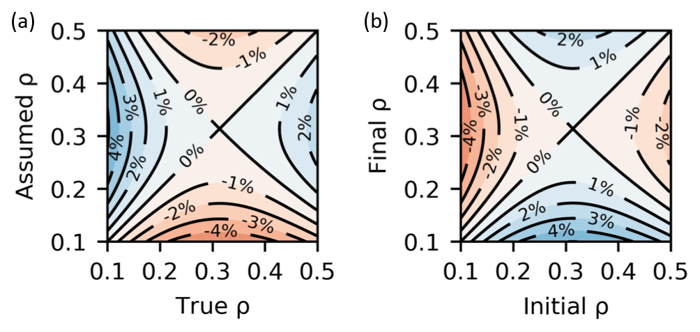
Figure 14 (a) Fractional ΔSWE estimation bias caused by misspecification of the snow density. (b) Apparent ΔSWE caused by a bulk snowpack density change in the absence of actual SWE change, as a fraction of total actual SWE.

In the absence of any ΔSWE, snowpack evolution may result in a bulk ρ change (e.g., due to settling) which will cause a Φ_s contribution. This contribution will be spuriously attributed to a SWE change. Consider the case of a snowpack with total SWE of S that undergoes a ρ change from initial ρ₁ to final ρ₂. According to Eq. (5), this will cause a Φ_s change:

$$\begin{array}{}\text{(21)}& {\mathrm{\Phi }}_{\mathrm{s}}=S\left(\mathit{\xi }\right({\mathit{\rho }}_{\mathrm{2}})-\mathit{\xi }({\mathit{\rho }}_{\mathrm{1}}\left)\right).\end{array}$$

Assuming that the temporal mean ρ of $({\mathit{\rho }}_{\mathrm{1}}+{\mathit{\rho }}_{\mathrm{2}})/\mathrm{2}$ is somehow known and used for estimation, the resulting ΔSWE error, S_e, as a fraction of total SWE will be

$$\begin{array}{}\text{(22)}& {\displaystyle \frac{S_e}{S}}=\mathrm{2}{\displaystyle \frac{\mathit{\xi }\left({\mathit{\rho }}_{\mathrm{2}}\right)-\mathit{\xi }\left({\mathit{\rho }}_{\mathrm{1}}\right)}{\mathit{\xi }\left({\mathit{\rho }}_{\mathrm{1}}\right)+\mathit{\xi }\left({\mathit{\rho }}_{\mathrm{2}}\right)}}.\end{array}$$

This fractional error is shown in Fig. 14b for initial and final ρ over the interval [0, 0.5]. This shows that a ρ increase or decrease will, respectively, cause a negative or positive ΔSWE error. Since snowpack evolution generally results in densification, this effect will tend to negatively bias estimated ΔSWE. However, for the considered ρ range, the bias is < 5 % of the total SWE.

For simplicity we assumed a value of ρ = 0.3 for all ΔSWE estimates. This value is likely too large for the dry-snow season in Inuvik. For example, the mean snow density measured across all transects summarized in Table 2 is ρ = 0.17, and according to Eq. (20), the use of the assumed value results in a 2.1 % bias which is small compared to the other errors discussed in Sect. 5. This small bias could be mostly mitigated by assuming a more appropriate ρ according to the location and time of year (e.g., Sturm and Wagner, 2010).

Regarding the effect of vertical density layering, our study area is prone to wind slab formation in which the late season snowpack can consist of a dense wind slab overlaying a low-density hoar layer (Rutter et al., 2019; King et al., 2018). Considering the extreme case of near-zero density hoar overlain by ρ = 0.5 wind slab, assuming a uniform ρ = 0.3 results in a +2.5 % estimation bias which is still a small error compared to the other bias sources considered in our analysis.

5.2 Violation of ΔSWE horizontal homogeneity assumption

Temporal changes in SWE can be caused by a number of different processes including deposition of new snow, as well as redistribution by wind, melt, and sublimation. Each of these processes is spatially modulated in natural terrain by the configuration of topography and vegetation (Morse et al., 2012; Anderton et al., 2004; Palmer et al., 2012). Furthermore, vegetation distribution is itself modulated by topography (Walker, 2000). For these reasons, spatial variation in ΔSWE over a particular time period is likely to show some correlation with topography, either directly with elevation or with derived indices such as slope, aspect, or measures of curvature.

As shown in Sect. 3.3, the estimation of ΔSWE within a spatial window through the correlation with $\stackrel{\mathrm{̃}}{\mathit{\xi }}$ is subject to bias when there are horizontal ΔSWE variations within the window that are correlated with either $\stackrel{\mathrm{̃}}{\mathit{\xi }}$ itself or with ${\stackrel{\mathrm{̃}}{\mathit{\xi }}}^{\mathrm{2}}$. To investigate the significance of this effect, we simulated the seasonal evolution of spatially variable ΔSWE distributions due to variations in topography and vegetation using SnowModel (Liston and Elder, 2006), implemented as a Fortran software package that includes sub-models for metrological forcing conditions, surface energy exchanges, snowpack evolution, and 3D wind transport. We simulated an evolving snowpack over several snow seasons for two cases: (1) bare-earth case with no snow-holding vegetation to examine the impact of topographic variation only, and (2) spatially variable vegetation heights (i.e., variable snow-holding capacity) to consider the additional influence of vegetation. The spatially varying vegetation was modelled using the NALCMS 2015 land-classification data for our study area.

We chose a study area and time period for the simulation that correspond to the spatial footprint and a similar time period as the RS2-SLA dataset we used for the method demonstration described in Sect. 2.1. SnowModel also takes as input the digital elevation model of the study area and one or more time series of meteorological driving data in the form of regularly sampled temperature, wind, and precipitation data. We ran the model using the same 12 m TanDEM-X DEM used for InSAR topographic phase correction and SWE change estimation. Therefore, the model did not simulate variations in SWE at scales finer than 12 m. Note that spatial SWE variations finer than the resolution of the SlopeVAR input data, ξ and ϕ, will not bias the estimates but instead will contribute to phase decorrelation and therefore affect the estimation variance, as discussed in Sect. 3.6.

Meteorological forcing data was input from three locations: (1) Environment and Climate Change Canada (ECCC) Inuvik climate station (68.32^∘ N, 133.53^∘ W), adjacent to position “E” in Fig. 1a and 6 km from the scene center (ECCC, 2021b); (2) ECCC Trail Valley Creek station (68.74^∘ N, 133.50^∘ W), 43 km north of the scene center; and (3) the Government of Northwest Territories – Department of Environment and Natural Resources (GNWT-ENR) southern ITH station (68.54^∘ N, 133.77^∘ W), 21 km north of the scene center (dataset provided directly from GNWT-ENR). SnowModel weights the station inputs according to an inverse distance squared parameter, and therefore the Inuvik Climate Station dominates the model input. The model was run with default settings at a daily time step interval with results output every 24 d corresponding to the imaged dates of the RS2-SLA dataset. The resulting absolute SWE maps, produced in the original DEM spatial reference, were resampled to the RS2-SLA range–Doppler geometry and sequentially differenced to produce 24 d ΔSWE maps.

These ΔSWE maps were then used along with the ξ map, computed from the DEM with a nominal value of ρ=0.3, to determine the expected ${\widehat{\mathrm{\Delta }S}}_{\mathrm{w}}$ error according to the first two terms in Eq. (13), i.e., those related to $\stackrel{\mathrm{̃}}{\mathrm{\Delta }S}$. The modelled ΔSWE error maps were computed with rectangular estimation windows with 500 m × 500 m ground footprint.

Figure 15 Results for ΔSWE simulation for the bare ground (top row) and NALCMS 2015 vegetation distribution (bottom row) cases for the RS2-SLA geometry over Inuvik for the period 17 July 2011 to 29 April 2020. Sequential 24 d ΔSWE values were simulated for the dry-snow season each year (nominally chosen to be 1 October to 31 March according to Fig. 2) resulting in a total of sixty 24 d intervals being simulated. Panels (a) and (d) are temporal means of the expected ΔSWE error, (b) and (e) are histograms of all expected errors (all spatial estimates over all time intervals), and (c) and (f) are histograms of the spatial mean ΔSWE error for the set of intervals. Water areas are greyed out.

We analyzed our simulations for all 24 d intervals from 17 July 2011 to 29 April 2020 falling within the expected dry-snow season, nominally chosen to be 1 October to 31 March of each year based on the climate normals for Inuvik (see Fig. 2). The results, summarized in Fig. 15, show the spatial distribution of the ΔSWE error averaged over all modelled time intervals and histograms of all expected ΔSWE errors and the per-interval spatially averaged mean ΔSWE error.

For the bare-earth case (Fig. 15a–c), a single outlier interval (5 January 2012 to 29 January 2012) was omitted from the summary analysis because the errors for that interval were very large compared to all other intervals. This appears to be due to a strong correlation of the simulated spatial ΔSWE distribution with $\stackrel{\mathrm{̃}}{\mathit{\xi }}$ for that 24 d interval which can occur when a strong wind-transport event directionally aligns with the horizontal projection of the SAR line-of-sight. Hence, the simulated topography-modulated scouring and deposition along the wind-direction axis can, by chance, align with the SAR geometry ground-range direction which results in a very large estimation bias. It may be possible to detect these events by analysis of the wind history (e.g., thresholding of a suitable blown-snow index while also considering the wind direction with respect to the SAR ground-range direction). We investigated this approach by computing the time-varying blowing snow probability as modelled by Li and Pomeroy (1997) which provides the probability that blowing snow conditions will occur as a function of wind speed and temperature. We computed these at daily time steps, assigned the mean wind direction to each time step, and then integrated these 2D vectors over the 24 d simulation intervals. The result is a directional cumulative blowing snow index in units of hours (of blowing snow) and is shown in Fig. 16 for all simulated 24 d intervals. This shows that the SnowModel outlier case is also an outlier with respect to the blowing snow index magnitude (and also when projected to the SAR look direction axis) suggesting that wind-driven redistribution is responsible for the predicted large ΔSWE bias.

Another potential mitigation is to use SAR images from the opposite pass direction. The bias from the near-opposite horizontal direction should have the opposite sign, and therefore the estimated ΔSWE should differ significantly between pass directions, allowing for the effect to be detected and perhaps mitigated by averaging the results.

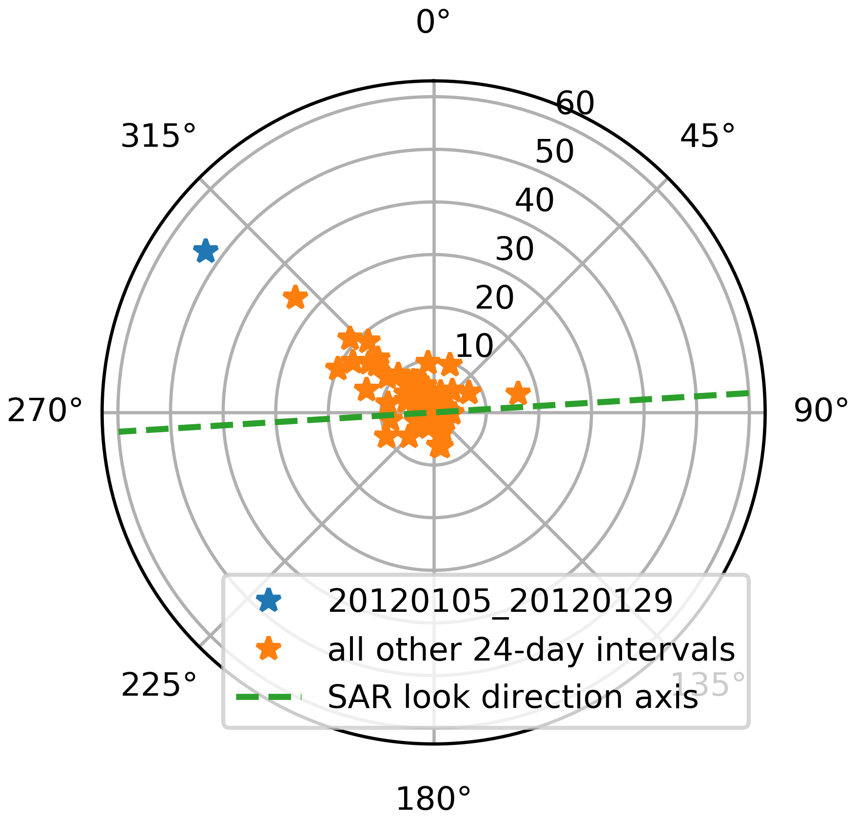
Figure 16 Directional cumulative blowing snow hours computed using ERA-5 surface parameters applied to the Li and Pomeroy (1997) probability model for all simulated 24 d intervals. The 20120105_20120129 interval appears as an outlier with respect to the cumulative magnitude. The SAR look direction axis is shown for comparison.

For the bare-ground case, the temporal mean ΔSWE error map shows mean errors in the ± 2 mm range with spatial features (Fig. 15a) that are generally aligned with topographic variations (Fig. 1b). The distribution of all ΔSWE errors (Fig. 15b) has a mean of just −0.2 mm which corresponds to a small negative overall estimation bias and an RMS value of 2.0 mm which corresponds to approximately 20 % of the simulated mean per-interval ΔSWE value. The histograms of the per-interval spatially averaged errors (Fig. 15c) show that the majority of 24 d intervals have a mean error near zero, suggesting that averaging estimates over wider areas reduces the bias effect introduced by spatially variable ΔSWE distribution.

For the NALCMS 2015 vegetation case, the temporal mean ΔSWE error map (Fig. 15d) shows mean errors with magnitudes that are much larger than for the bare-earth case (up to 100 mm in some areas) corresponding to areas with heterogenous vegetation classifications (see Fig. 1c). The distribution of ΔSWE errors (Fig. 15e and f) has a mean and RMS value of 4.3 mm and 39.6 mm which are very substantial. This suggests that spatially varying vegetation snow-holding conditions may substantially bias the ΔSWE estimates. However, it should be noted that results from real data, presented in Sect. 4, do not show such large variations as would be expected by the error magnitudes in Fig. 15d–f. The reason could be that the simulation driven by the NALCMS vegetation classification significantly over-represents the effect of spatially variable vegetation. Nevertheless, these results highlight the relative importance of vegetation as a source of method bias and suggest that some form of mitigation may be required to yield useful estimates from the proposed method in areas with variable vegetation snow-holding heights.

We compared the relative values of the $\langle \mathit{\xi }\rangle \langle \stackrel{\mathrm{̃}}{\mathit{\xi }}\stackrel{\mathrm{̃}}{\mathrm{\Delta }S}\rangle$ and $\langle {\stackrel{\mathrm{̃}}{\mathit{\xi }}}^{\mathrm{2}}\stackrel{\mathrm{̃}}{\mathrm{\Delta }S}\rangle$ contributions to the ΔSWE error which showed that for all 24 d intervals, and both bare-earth and NALCMS 2015 cases, the RMS of the $\langle \mathit{\xi }\rangle \langle \stackrel{\mathrm{̃}}{\mathit{\xi }}\stackrel{\mathrm{̃}}{\mathrm{\Delta }S}\rangle$ component was much greater than that of the $\langle {\stackrel{\mathrm{̃}}{\mathit{\xi }}}^{\mathrm{2}}\stackrel{\mathrm{̃}}{\mathrm{\Delta }S}\rangle$ component so that with respect to the influence of $\stackrel{\mathrm{̃}}{\mathrm{\Delta }S}$, the spatial correlation with respect to ${\stackrel{\mathrm{̃}}{\mathit{\xi }}}^{\mathrm{2}}$ can be neglected.

5.3 Correlated phase components

As shown in Eq. (12), additional phase components, other than Φ_s, will contribute to ${\widehat{\mathrm{\Delta }S}}_{\mathrm{w}}$ error according to their spatial correlation with $\stackrel{\mathrm{̃}}{\mathit{\xi }}$: $\langle \stackrel{\mathrm{̃}}{\mathit{\xi }}{\mathrm{\Phi }}_{\mathrm{e}}\rangle /\langle {\stackrel{\mathrm{̃}}{\mathit{\xi }}}^{\mathrm{2}}\rangle$. We distinguish between (1) systematic spatial correlation between ξ and the Φ_e components that have a topographic dependence and (2) spurious correlations with Φ_e components that are not systematically dependent on topography. In this section we consider the former by examining several Φ_e components, their spatial characteristics with respect to topographic slope, and their expected contribution to ${\widehat{\mathrm{\Delta }S}}_{\mathrm{w}}$ error.

Φ_e components not systematically correlated with $\stackrel{\mathrm{̃}}{\mathit{\xi }}$ will contribute to the ${\widehat{\mathrm{\Delta }S}}_{\mathrm{w}}$ error due to finite sampling over the estimation window. These include decorrelation phase noise and the non-$\stackrel{\mathrm{̃}}{\mathit{\xi }}$-correlated parts of other phase components. In the case of these spurious correlations, the resulting estimation error magnitude can be expected to diminish with larger estimation window sizes and, in the global sense, will not systematically bias the estimates but instead contribute to the variance.

5.3.1 Atmospheric delay

The troposphere contributes substantial phase delay during SAR imaging (Hanssen, 2001). This delay can be decomposed into static and dynamic components. Temporal differences in the static component between image acquisitions results in a Φ_e component that is modulated by topography. Neglecting any height dependence of the delay over the height range within the estimation window, the static atmospheric phase contribution (Φ_sa) can be modelled as a simple linear function (Lin et al., 2010),

$$\begin{array}{}\text{(23)}& {\mathrm{\Phi }}_{\text{sa}}={\displaystyle \frac{\mathrm{4}\mathit{\pi }}{\mathit{\lambda }}}\mathrm{\Delta }Kh+\mathit{\beta },\end{array}$$

where ΔK is the linear transfer function coefficient corresponding to the volumetric mean delay difference between SAR acquisitions, h is the topographic height, and β is an offset constant which we set to zero without loss of generality since we consider only the correlation of Φ_sa with zero-mean $\stackrel{\mathrm{̃}}{\mathit{\xi }}$. Note that the horizontal variation in ΔK is gradual, and therefore ΔK can be assumed constant within the estimation window. Therefore, the spatial variation in Φ_sa within the ΔSWE window (assumed to be ≤ 1 km as discussed in Sect. 5.5) can be attributed solely to variation in h.

The dynamic component is driven by turbulent mixing, and therefore its spatial power spectrum follows a power-law relationship, which limits the amplitude at spatial scales below a few kilometres (Hanssen, 2001). Therefore, for estimation windows < 1 km, the dynamic component can reasonably be neglected. For larger estimation windows (not explicitly considered in this paper), the influence of the dynamic component can be mitigated by spatial high-pass filtering both the InSAR phase and ξ prior to ΔSWE estimation, similar to the method employed by Lin et al. (2010) for estimating ΔK from interferograms.

Figure 17 Expected contribution of topographically correlated phase components to ${\widehat{\mathrm{\Delta }S}}_{\mathrm{w}}$ error. Panels (a) and (b) show the error due to a static atmospheric volumetric delay error of ΔK = 10⁻⁵, (c) and (d) show the error per 10 mm of surface heave over the time interval, discussed in Sect. 5.3.2, and (e) and (f) show the error for the reference solifluction case (d_sf = 10 mm ⋅tan α), discussed in Sect. 5.3.3. Water areas are greyed out.

Figure 17a and b show the expected ${\widehat{\mathrm{\Delta }S}}_{\mathrm{w}}$ error for the case of ΔK = 10⁻⁵ (i.e., 10 mm km⁻¹). For this case the RMS error is 1.1 mm. However, the distribution is centered around zero so that the mean error is only 0.04 mm. Therefore, spatial averaging of the estimates over a sufficient area will tend to mitigate the error due to static atmospheric delay.

Regarding the temporal distribution of ΔK, given that it is a pairwise differential quantity, it has zero expectation on an annualized timescale. However, there is some seasonal dependence on tropospheric delay (Cong et al., 2012), and therefore ΔK, for sequential dry-snow-season interferograms, should not be considered temporally random. For a particular spatial location, the errors may accumulate constructively over a snow season to yield a consistent, albeit small, bias effect for that location. However, methods exist for the estimation of ΔK either by correlation with topographic height over estimation windows corresponding to the full-scene or tens of kilometres (Lin et al., 2010; Bekaert et al., 2015) or from climate reanalysis data (Cong et al., 2012). Therefore, interference from Φ_sa is not considered a limiting factor for the proposed method since the effect can be largely mitigated.

5.3.2 Surface displacement

Surface displacements may result from freezing that causes upward heave and thawing that causes downward subsidence. Surface displacements associated with freezing or thawing are predominantly in the direction of the local surface normal, and therefore spatial variation in the InSAR phase signal induced by such displacement (Φ_he) is approximated by

$$\begin{array}{}\text{(24)}& {\mathrm{\Phi }}_{\text{he}}=-{\displaystyle \frac{\mathrm{4}\mathit{\pi }}{\mathit{\lambda }}}{d}_{\mathrm{h}}\cos \mathit{\theta },\end{array}$$

where d_h is the displacement magnitude away from the reference surface, with positive and negative displacements, respectively, corresponding to freezing (heave) and thawing (subsidence).

In equilibrium climate conditions, seasonal active-layer displacement tends to follow a pattern of heave in early to mid-winter related to freeze-back to the top of permafrost, which is followed by static conditions until the spring. Then the active layer thaws gradually throughout the summer. Therefore, the dry-snow season can be divided into an initial period of positively valued displacement followed by a static period. Longer-term positively or negatively valued displacement may be superimposed onto this seasonal pattern due to changes in permafrost conditions. Annual displacement amplitudes for seasonally frozen terrain typically occur in the range of 20 to 120 mm (Gruber, 2020).

Areas with heavily organic soil (e.g., peat) can have significantly higher seasonal displacements. In the vicinity of the study area, we have observed that these occur in localized areas without significant topographic variation, i.e., areas already not well suited for the method because of limited ξ diversity. It may be possible to exclude these areas by masking based on local ξ diversity or analysis of summer interferograms (we have observed that these areas tend to have low temporal coherence due to their significant displacement phase).

To assess the significance of heave as an interfering factor we consider a reference case in which d_h = 10 mm over a 24 d interval. Figure 17c and d show the expected ${\widehat{\mathrm{\Delta }S}}_{\mathrm{w}}$ error for this reference case. The error is always positively valued and corresponds to an approximately +9 mm ΔSWE bias over the 24 d estimation interval which is very substantial, considering that 24 d ΔSWE values are typically < 20 mm for the study area (see Fig. 12). Hence, there is potential for displacement processes, if present, to significantly interfere with the proposed estimation method. Regarding whether we can assume that d_h is constant over the estimation window, surface conditions affecting heave can certainly vary at scales shorter than the 500 m window size, e.g., as observed by Liu et al. (2012), and this spatial variability will contribute to estimation error to some degree, although we have not attempted to quantify this effect.

Regarding the results presented in Sect. 4.3, the ΔSWE values are expected to yield a positive bias until freeze-back of the active layer is completed. Considering the reference case presented here in which 10 mm of heave results in a mean ΔSWE bias of 9 mm, the October–December bias can be explained by $(\mathrm{8.6}\mathrm{mm}/\mathrm{0.9})(\mathrm{92}\mathrm{d}/\mathrm{24}\mathrm{d})$ = 37 mm of mean upward displacement amplitude, which is a plausible value for the area during active-layer freeze-back (Gruber, 2020).

The +1.7 mm bias for the snow-free periods presented in Sect. 4.3 is unexpected since the snow-free period is expected to correspond to subsidence and therefore a negative bias with magnitude similar to but less than October–December because the subsidence is expected to occur over a longer time interval than the re-freeze. This disagreement suggests other factors that are difficult to separate from one another; perhaps the thaw is directionally asymmetric with the heave (i.e., contribution from solifluction) as described in Sect. 5.3.3.

One mitigation approach is to limit use of the estimator spatially and temporally to correspond to known areas and periods of low displacement activity. For example, temporal analysis of summer interferograms can be used to identify areas with significant subsidence, and these can be masked out during ΔSWE estimation under the assumption that thaw-period subsidence is spatially correlated with freeze-period heave. Of course, this is not possible for the case of widespread seasonal surface displacement as is common in periglacial regions. Such areas are relatively common (e.g., Obu et al., 2019, report that 22 % of the exposed land area of the Northern Hemisphere potentially contains permafrost). It may also be possible to estimate and correct for the early winter heave component by estimating the thaw subsidence from summer-season interferograms and then applying a model for the cyclical deformation.

5.3.3 Solifluction

We consider slow-moving, gravity-driven surface soil flux, i.e., solifluction, as a potential Φ_e component since it is correlated with topographic slope. We do not expect solifluction to be a significant bias source during the dry-snow season but include it because it may affect snow-free interferograms analyzed for the purpose of method validation.

Solifluction is driven by cyclical surface displacement (diurnal or seasonal) coupled with sufficient topographic slope magnitude and surface conditions (Matsuoka, 2001), and it is common in periglacial regions. The flow direction is principally in the local downslope direction, and therefore the resulting InSAR phase (Φ_sf) is approximated by

$$\begin{array}{}\text{(25)}& {\mathrm{\Phi }}_{\text{sf}}={\displaystyle \frac{\mathrm{4}\mathit{\pi }}{\mathit{\lambda }}}{d}_{\text{sf}}(\mathit{l}\cdot \mathit{d}),\end{array}$$

where d_sf is the downslope surface displacement magnitude due to solifluction, and l and d are the unit magnitude SAR line-of-sight and downslope direction vectors. Spatial variation in d_sf can be modelled as a function of d_h and α only. An upper bound for d_sf suggested by Matsuoka (2001) on an annualized basis is

$$\begin{array}{}\text{(26)}& d_{\text{sf}}\le d_{\text{h}}\tan \mathit{\alpha },\end{array}$$

which attributes downslope soil motion to the heave process minus any retrograde motion due to soil cohesion. In order to assess the significance of solifluction as an interfering factor we consider a reference case in which d_sf = 10 mm ⋅tan α. Figure 17e and f show the expected ${\widehat{\mathrm{\Delta }S}}_{\mathrm{w}}$ error for this reference case. The error is always positively valued and corresponds to a 0.6 mm bias per 10 mm heave on an annualize basis, which is significantly less than that due directly to heave discussed in Sect. 5.3.2.

5.3.4 Soil moisture

Near-surface soil moisture conditions are a known contributor to the InSAR phase signal (Nolan et al., 2003), and these are likely modulated by topographic slope both in terms of gravity-driven effects on near-surface hydrology and the influence of slope aspect on solar heating. As such, there may be some correlation with ξ leading to estimation bias. As with solifluction, we do not expect soil moisture to significantly affect dry-snow interferograms but consider its effect on snow-free interferograms used as method validation controls.

Although the correlation of soil moisture phase with topographic slope is difficult to model, it is possible to establish a bound on its impact on ${\widehat{\mathrm{\Delta }S}}_{\mathrm{w}}$ by considering that the soil moisture phase magnitude, Φ_sm, is limited to some maximum value, Φ_{sm_max}, according to sensor wavelength and soil type (De Zan et al., 2014). Considering a case where $\mathit{\xi }\in [{\mathit{\xi }}_{min},{\mathit{\xi }}_{max}]$, the spatial distribution of Φ_sm producing maximum possible ${\widehat{\mathrm{\Delta }S}}_{\mathrm{w}}$ bias is

$$\begin{array}{}\text{(27)}& {\mathrm{\Phi }}_{\text{sm}}={\mathrm{\Phi }}_{\text{sm\_max}}{\displaystyle \frac{\mathit{\xi }-{\mathit{\xi }}_{min}}{{\mathit{\xi }}_{max}-{\mathit{\xi }}_{min}}},\end{array}$$

which corresponds to perfect correlation between Φ_sm and ξ. According to Eq. (12) this yields a ΔSWE bias limit of ${\mathrm{\Phi }}_{\text{sm\_max}}/({\mathit{\xi }}_{max}-{\mathit{\xi }}_{min})$. Considering our study case, ξ∈ [0.22 rad mm⁻¹, 0.28 rad mm⁻¹ ] (see Fig. 6a), and assuming Φ_{sm_max} = 90^∘, which is reasonable considering the model of De Zan et al. (2014) and the simulation results from Rabus et al. (2010), this corresponds to a bias magnitude limit of 1.3 mm which is relatively small especially when considering that any actual spatial correlation is likely much less than this ideal upper limit.

5.4 DEM error

Errors in the DEM used for analysis contribute to the ${\widehat{\mathrm{\Delta }S}}_{\mathrm{w}}$ error due to both the residual topographic phase, as a component of Φ_e, and error in $\stackrel{\mathrm{̃}}{\mathit{\xi }}$ used by the estimator.

The topographic phase error (Φ_topo) scales linearly with both perpendicular orbit baseline, B_⊥, and DEM error, Δh. Considering the Φ_e term in Eq. (13) and the fact that Δh varies spatially, the resulting ΔSWE bias scales with $E\left(B_{\perp }\right)E(\langle \stackrel{\mathrm{̃}}{\mathit{\xi }}\mathrm{\Delta }h\rangle )$ with respect to all interferograms. We assume that E(B_⊥) is zero for a sensor with a maintained orbit, and therefore this effect is likely unbiased with respect to a temporal set of ΔSWE maps.

Next, we consider the effect of errors in $\stackrel{\mathrm{̃}}{\mathit{\xi }}$ caused by DEM errors. The estimator defined in Eq. (12) can be better expressed using the DEM-derived ${\stackrel{\mathrm{̃}}{\mathit{\xi }}}_D=\stackrel{\mathrm{̃}}{\mathit{\xi }}+{\stackrel{\mathrm{̃}}{\mathit{\xi }}}_{\mathrm{\Delta }h}$ instead of true $\stackrel{\mathrm{̃}}{\mathit{\xi }}$, in which ${\stackrel{\mathrm{̃}}{\mathit{\xi }}}_{\mathrm{\Delta }h}$ is the error in ${\stackrel{\mathrm{̃}}{\mathit{\xi }}}_D$. As a first-order analysis of this error, we neglect the second-order terms involving both ${\stackrel{\mathrm{̃}}{\mathit{\xi }}}_{\mathrm{\Delta }h}$ and the bias terms in Eq. (12). Therefore,

$$\begin{array}{}\text{(28)}& \widehat{\mathrm{\Delta }S}={\displaystyle \frac{〈{\stackrel{\mathrm{̃}}{\mathit{\xi }}}_D\stackrel{\mathrm{̃}}{\mathrm{\Phi }}〉}{〈{\stackrel{\mathrm{̃}}{\mathit{\xi }}}_D^{\mathrm{2}}〉}}\cong \langle \mathrm{\Delta }S\rangle \left({\displaystyle \frac{〈{\stackrel{\mathrm{̃}}{\mathit{\xi }}}^{\mathrm{2}}〉+〈\stackrel{\mathrm{̃}}{\mathit{\xi }}{\stackrel{\mathrm{̃}}{\mathit{\xi }}}_{\mathrm{\Delta }h}〉}{〈{\stackrel{\mathrm{̃}}{\mathit{\xi }}}^{\mathrm{2}}〉+〈{\stackrel{\mathrm{̃}}{\mathit{\xi }}}_{\mathrm{\Delta }h}^{\mathrm{2}}〉+\mathrm{2}〈\stackrel{\mathrm{̃}}{\mathit{\xi }}{\stackrel{\mathrm{̃}}{\mathit{\xi }}}_{\mathrm{\Delta }h}〉}}\right).\end{array}$$

If we assume that ${\stackrel{\mathrm{̃}}{\mathit{\xi }}}_{\mathrm{\Delta }h}$ is uncorrelated with $\stackrel{\mathrm{̃}}{\mathit{\xi }}$,

$$\begin{array}{}\text{(29)}& \widehat{\mathrm{\Delta }S}\cong \langle \mathrm{\Delta }S\rangle \left(\mathrm{1}-{\displaystyle \frac{〈{\stackrel{\mathrm{̃}}{\mathit{\xi }}}_{\mathrm{\Delta }h}^{\mathrm{2}}〉}{〈{\stackrel{\mathrm{̃}}{\mathit{\xi }}}^{\mathrm{2}}〉+〈{\stackrel{\mathrm{̃}}{\mathit{\xi }}}_{\mathrm{\Delta }h}^{\mathrm{2}}〉}}\right),\end{array}$$

which corresponds to a multiplicative bias towards lower amplitudes that is more pronounced in areas with low ξ variance. We have not attempted to quantify $\langle {\stackrel{\mathrm{̃}}{\mathit{\xi }}}_{\mathrm{\Delta }h}^{\mathrm{2}}\rangle$ for our TanDEM-X DEM-derived ξ map, but we made efforts to reduce it by smoothing the DEM (see Sect.  3.5), noting that this approach has its limits since over-smoothing will tend to increase $\langle {\stackrel{\mathrm{̃}}{\mathit{\xi }}}_{\mathrm{\Delta }h}^{\mathrm{2}}\rangle$. Note that smoothing the DEM has the benefit of reducing potential bias introduced by short-scale horizontal heterogeneity in the snowpack (e.g., those noted by Sturm and Benson, 2004). Instead, the effect of these variations will be limited to an increase in the uncorrelated phase components discussed in Sect. 3.6.

Regarding requirements for DEM generation frequency to accommodate landform changes, at the scale applied in our study (DEM smoothed to 90 m resolution), DEM generation frequency can likely be > 10 years. However, if applying the method using more finely scaled data, a more recent DEM may be required since fine-scale landform changes occur more frequently.

5.5 Spatial resolution and geographic suitability

Regarding the choice of estimator window size, larger windows improve precision by mitigating the effect of spatially random noise. However, as discussed in Sect. 5.3, increasing window size does not necessarily mitigate deterministic bias contributions. Therefore, in terms of the trade-off between estimator error and spatial resolution, there is an upper limit for which increasing window size will significantly reduce the expected error. For our study dataset we empirically determined 500 m to be best choice for the window size since larger windows did not yield significant reductions in the observed spatial variance of ΔSWE estimates.

As discussed in Sect. 3.6, the precision of the SlopeVar estimator depends on both the coherence level and the local ξ variance. These factors are spatially variable, and therefore in order to generalize the achievable spatial resolution to other locations, one needs to consider both the degree of topographic slope variation and conditions affecting coherence (e.g., vegetation). Within a single dataset, this heteroskedasticity of the estimator could be addressed by applying an adaptively sized estimation window during the estimation to achieve approximately uniform variance but variable spatial resolution, in other words, growing the window size to compensate in areas of low ξ diversity. Another approach would be to simply mask out areas expected to have high variance based on coherence or ξ diversity.

These considerations affect the geographic suitability of the method; it requires dry-snow conditions and at least moderate topographic variation. Such conditions are present at least part of the time in many geographic regions. The method is less suitable in areas with frequent wet-snow conditions such as coastal areas and in regions that are mostly flat, such as prairie.

5.6 Correcting for the dry-snow phase component

The main focus of this article is the estimation of ΔSWE. However, for repeat-pass InSAR applications other than ΔSWE estimation (e.g., surface deformation estimation), Φ_s can be considered an interfering factor. In this case, knowing the spatial ΔSWE distribution for a given interferogram allows for removal of Φ_s according to Eq. (5). Furthermore, ΔSWE can, in principle, be estimated at scales finer than the SlopeVar estimation window size by (1) first using SlopeVar to generate a coarse-scale estimate, (2) removing Φ_s corresponding to this initial estimate, and then (3) attributing the remaining phase to additional (high-spatial-frequency) ΔSWE which can then be estimated per resolution cell according to Eq. (5). We performed a preliminary investigation of this by scaling the ${\widehat{\mathrm{\Delta }S}}_{\mathrm{w}}$ maps by the ξ map to generate spatial maps of estimated Φ_s and then demodulating the original interferograms. The result was, in general, a significant increase in observed spatial phase gradients and short-scale phase artifacts likely because of short-scale errors in the ${\widehat{\mathrm{\Delta }S}}_{\mathrm{w}}$ maps. This approach therefore requires further investigation because, in order to maintain spatial phase smoothness required for subsequent phase unwrapping, the ΔSWE maps likely require imposition of smoothness constraints.

6 Conclusions

We have introduced a novel spatial analysis method, “SlopeVar”, that estimates dry SWE change from wrapped repeat-pass interferograms by spatially correlating the InSAR phase to a DEM-derived, slope-dependent dry-snow phase sensitivity map over a suitably sized estimation window. The method does not require phase unwrapping or any spatial reference with known SWE change and therefore addresses some of the key challenges posed by InSAR-based SWE change estimation.

We tested our method using a 9-year stack of RADARSAT-2 Spotlight-A mode images over an area surrounding the town of Inuvik, Northwest Territories, Canada, and corresponding TanDEM-X DEM for the area. We generated SlopeVar ΔSWE maps from the dataset for both snow-covered and snow-free periods and compared these with a number of in situ SWE transect measurements made over two winters, and the results showed good agreement with an absolute SWE RMSE of 15 mm. We compared our spatially averaged results with the ERA5 ΔSWE time history, and the results showed a moderately strong correlation and 7.9 mm RMSE (per 24 d period) over the October–March period. Seasonal analysis revealed a substantial early winter (October–December) bias (8.5 mm per 24 d period) that is largely absent in late winter (January–March), which we suspect is due to seasonal active-layer heave.

We empirically determined that a 500 m estimation window size provides the best combination of error mitigation and spatial resolution for our dataset. However, the achievable spatial resolution depends both on terrain factors affecting the coherence and on the degree of slope variation, both of which are location-dependent.

The method is subject to bias from factors that spatially correlate with the dry-snow phase sensitivity map. We investigated the role of spatial SWE change inhomogeneity as a possible bias factor and determined that vegetation homogeneity should be controlled for during estimation, e.g., by limiting the estimator to homogenous areas. We investigated the role of static atmospheric delay and surface deformation as potential bias factors and also investigated solifluction and soil moisture phase, two bias sources expected to only affect snow-free interferograms used as zero ΔSWE controls for method validation. We found that static atmospheric delay, soil moisture, and solifluction are likely not significant sources of bias and that surface deformation due to heave, if present, may lead to substantial estimation bias. We also considered the effect of DEM error and found that DEM errors lead to damping multiplicative ΔSWE bias, and therefore DEM filtering, pre-processing, or both should be performed to minimize this effect.

We compared the SlopeVar and Delta-K methods in terms of their relative achievable precision and found that, for our test area, SlopeVar is typically about 4× more precise than Delta-K for a given estimation window size. Regarding the benefits of the method compared to dual-frequency volume-scattering-based estimation, our method is less suitable in areas with relatively low topographic variation, although it may be possible to exploit even sparse areas of variation such as along waterways to sparsely map SWE change in otherwise flat areas. In other areas, the constraints are similar in that they both require dry-snow conditions, and there is opportunity for cross-validation in these areas. Our method has the advantage of only requiring a single band and is therefore feasible with existing spaceborne systems, especially L-band. In comparison to passive microwave-based estimation, we expect the SlopeVar method to perform better in high-relief areas which potentially offers complementary coverage in alpine regions that have previously been difficult areas to evaluate.