the Creative Commons Attribution 4.0 License.
the Creative Commons Attribution 4.0 License.
 | 27 Apr 2022
Influences of changing sea ice and snow thicknesses on simulated Arctic winter heat fluxes
Marika M. Holland
In the high-latitude Arctic, wintertime sea ice and snow insulate the relatively warmer ocean from the colder atmosphere. While the climate warms, wintertime Arctic surface heat fluxes remain dominated by the insulating effects of snow and sea ice covering the ocean until the sea ice thins enough or sea ice concentrations decrease enough to allow for direct ocean–atmosphere heat fluxes. The Community Earth System Model version 1 Large Ensemble (CESM1-LE) simulates increases in wintertime conductive heat fluxes in the ice-covered Arctic Ocean by ∼ 7–11 W m−2 by the mid-21st century, thereby driving an increased warming of the atmosphere. These increased fluxes are due to both thinning sea ice and decreasing snow on sea ice. The simulations analyzed here use a sub-grid-scale ice thickness distribution. Surface heat flux estimates calculated using grid-cell mean values of sea ice thicknesses underestimate mean heat fluxes by ∼16 %–35 % and overestimate changes in conductive heat fluxes by up to ∼36 % in the wintertime Arctic basin even when sea ice concentrations remain above 95 %. These results highlight how wintertime conductive heat fluxes will increase in a warming world even during times when sea ice concentrations remain high and that snow and the distribution of snow significantly impact large-scale calculations of wintertime surface heat budgets in the Arctic.
- Article
(8375 KB) - Full-text XML
-
Supplement
(1989 KB) - BibTeX
- EndNote


The Arctic is warming rapidly and much more rapidly than lower latitudes. This Arctic amplification (AA) is due to a combination of a number of related mechanisms, including sea ice loss, lapse rate and Planck feedbacks, and changing water vapor and clouds, among others (e.g., Graverson and Wang, 2009; Kumar et al., 2010; Screen et al., 2013; Pithan and Mauritsen, 2014; Vavrus, 2004; Feldl et al., 2020, Hall, 2004; Dai et al., 2019; Serreze and Barry, 2011). Sea ice loss contributes to increased surface warming through two primary methods: an albedo feedback and an insulating effect. The albedo feedback results from sea ice concentration losses that expose dark ocean water and sea ice surface state changes, including reduced snow cover and increased ponding, that darken the ice surface. These decrease the surface albedo and increase the surface absorption of incoming radiation. The insulating effect results from the thinning of the sea ice and overlying snow: in the winter, sea ice and snow insulate the relatively warmer ocean from the colder atmosphere. As sea ice and snow thin, more heat can be conducted through the sea ice to the atmosphere, influencing the ice–atmosphere exchange. Thinning ice and snow and increasing conductive heat fluxes can also lead to increased basal sea ice growth – a feedback in a warming world that is seen temporarily in climate projections before warming temperatures overwhelm this feedback and ice growth declines (e.g., Petty et al., 2018; Keen et al., 2021).
A large body of previous research has investigated the interactions between sea ice loss and AA. Most of the published research and the majority of the ongoing Polar Amplification Model Intercomparison Project (PAMIP) experiments focus on the influence of changes in sea ice concentration (SIC) on Arctic warming (e.g., Peings and Magnusdottir, 2014; Sun et al., 2015; Smith et al., 2019). Less attention has been paid to the influence of winter sea ice thinning on Arctic surface warming, in part because observations of sea ice thickness (SIT) have only recently become more readily available and in part because the effects of SIC losses tend to be large compared to those from SIT changes. Although wintertime SICs in the central Arctic remain high and have changed very little over the satellite era, the sea ice has thinned dramatically (e.g., Kwok and Rothrock, 2009; Kwok, 2018). Sea ice volume has decreased by roughly 66 % since submarines have been measuring (1958–1976) and by 50 % since 1999 (Kwok, 2018; Lindsay and Schweiger, 2015).
Recent work with atmosphere-only models over both the historical time period and future scenarios suggest that the atmospheric response to SIT changes are strongest in the cold season and at the surface, with atmospheric responses to SIT changes of similar or smaller magnitudes than the responses to SIC changes (e.g., Gerdes, 2006; Krinner, 2010; Lang et al., 2017; Labe et al., 2018b; Sun et al., 2018). There is qualitative agreement that the inclusion of SIT changes along with SIC changes leads to an enhancement of surface AA, although the range across different studies is large: two studies focused on the late 20th–early 21st centuries found annual AA enhanced by ∼37 %–50 % with the inclusion of SIT changes (Lang et al., 2017; Sun et al., 2018), whereas AA increased by ∼10 % in the future simulations (2051–2080) of Labe et al. (2018b).
Our understanding of the influence of SIT on winter surface AA is further complicated by the presence of snow on sea ice, as well as the heterogeneous distribution of both snow and sea ice thicknesses. Snow is a more effective insulator than sea ice – and relatively small changes in snow thicknesses can result in large changes in conductive heat fluxes through the ice with consequent impacts on ice–atmosphere exchange. To our knowledge, there have been relatively few basin-scale studies on the effects of snow on sea ice on the winter surface heat budgets in the Arctic in a changing climate. Previous work investigating SIT changes on winter Arctic warming have not typically considered the effects of changing snow cover and often exclude this in the experimental design. For example, Lang et al. (2017) used atmosphere-only models that do not allow for snow to accumulate on sea ice. Furthermore, previous work with atmosphere-only models specifies grid-cell average values for SIT, thus calculating conductive fluxes (which are inversely related to sea ice and snow thicknesses) from an average SIT rather than as a sum over a sub-grid-scale thickness distribution. This introduces errors relative to fully coupled model simulations which typically include a treatment of sub-grid-scale ice thickness variations. These sources of errors and uncertainties also apply to global reanalysis products, most of which use constant sea ice thicknesses and no snow on sea ice for their product estimates (e.g., Wang et al., 2019) and show particularly large errors over the Arctic Ocean (e.g., Bromwich et al., 2018; Jakobson et al., 2012, and references therein). In particular, the lack of snow on sea ice in reanalysis products and the influence on the conductive heat flux results in a warm bias relative to observations (Batrak and Müller, 2019).
In this study we investigate the influence of SIT, snow thickness, and heterogeneity in these fields on the Arctic winter energy budget in the climate modeling environment. We explore how projected thickness changes in both sea ice and snow influence conductive heat fluxes and ice–atmosphere heat exchange. We further investigate the importance of heterogeneity in sea ice and snow thicknesses at a model sub-grid-cell level and how this impacts conductive heat flux calculations and quantify the errors that are introduced by using grid-cell average SITs rather than heterogeneous fields. We explore how the wintertime Arctic heat fluxes change during a time period (1950–2070) when winter Arctic basin SICs remain high, while ice and snow show dramatic thinning. This allows us to elucidate the dynamic nature of the influence of sea ice and snow thicknesses on surface heat budget even when SIC changes are small. For context, we also compare results from the wintertime high-latitude Arctic to other seasons (fall) and regions that are undergoing rapidly changing SICs and associated changes in surface heat fluxes due to open-water formation.
2.1 CESM1-LE
We use the Community Earth System Model version 1 Large Ensemble (CESM1-LE; Kay et al., 2015) to explore relationships between Arctic wintertime conductive heat fluxes and sea ice and snow thickness fields. The CESM1-LE consists of 40 simulations forced with historical forcing from 1920–2005 and then the Representative Concentration Pathway 8.5 (RCP8.5) forcing from 2005–2100 (the no-mitigation scenario with a top-of-the-atmosphere radiative forcing of 8.5 W m−2 by 2100; Meinshausen et al., 2011). The sea ice model component (the Los Alamos Sea Ice Model, CICE; Hunke et al., 2017) in the CESM1 uses a sub-grid-scale ice thickness distribution (ITD) in which thermodynamics are calculated over five discrete sub-grid-cell thickness categories with minimum thickness bounds of 0, 0.64, 1.39, 2.47, and 4.57 m. The presence of the ITD influences both the mean climate state and climate feedbacks (Holland et al., 2006). The simulated ITD and sea ice concentrations within each category evolve through ice growth and melt, ridging due to mechanical forcing, and ice transport (e.g., Thorndike et al., 1975). The resulting concentrations of sea ice can range from 0 % to 100 % (although values of 100 % are rare due to lead formation) in the discrete thickness layers. Snowfall can accumulate on sea ice and be affected by snowmelt, ice ridging, and transport. Effectively this means that a different snow depth is present across the different ice thickness categories. Ice–atmosphere fluxes are calculated separately in each sea ice thickness category, weighted by the concentration in each category, and passed as grid-cell means to the flux coupler for use in the atmospheric model. CICE uses a multi-layer thermodynamic scheme (Bitz and Lipscomb, 1999; BL99) that includes the effects of a prescribed vertical salinity profile. Comparisons with the Pan-Arctic Ice-Ocean Modeling and Assimilation system (PIOMAS; Zhang and Rothrock, 2003) sea ice thickness reanalysis product show that the CESM1-LE and PIOMAS agree well for both summer and winter rates of sea ice volume change (Labe et al., 2018a). The CESM1-LE and PIOMAS also tend to agree on regional mean thicknesses and variabilities throughout much of the Arctic with the exception of the Canadian Archipelago and coastal Greenland, where the CESM1-LE overestimates sea ice volumes compared to PIOMAS (and PIOMAS underestimates volumes compared to buoy and submarine data).
2.2 Zero-layer thermodynamic conductive heat-flux model
Not all thermodynamic variables for individual ice thickness categories were saved as part of the CESM1-LE output. In order to disentangle the relative influences of sea ice and snow thicknesses and their distributions, we use the available CESM1 output along with the zero-layer thermodynamic model of Semtner (1976) to estimate the conductive heat flux. This simple zero-layer model – developed originally to minimize computational costs associated with ice thickness calculations in climate models – assumes a linear temperature gradient through the sea ice and snow, and that the conductive heat flux through the ice + snow layer is
where Ks and Ki are the snow and ice conductivities of heat (0.3 Wm−1 K−1 and 2.0 Wm−1 K−1), hs and SIT are the snow and ice thicknesses, and Tb and Ts are temperatures at the bottom (ocean–ice) and surface (ice–atmosphere) of the ice.
The conductive heat flux reduces to
where and heff= (SIT + (Kratio⋅hs)), which is a measure of the effective thickness from an insulating perspective, with .
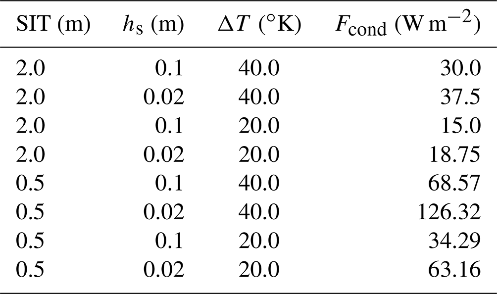
In the Arctic winter, surface temperatures are cold – well below the melting point of ice and snow – and the net surface energy budget (the sum of the net short- and longwave radiation and sensible and latent heat fluxes) in ice-covered regions is balanced by the conductive heat flux from the ocean through the sea ice and snow. Where open water is present, such as leads in the sea ice, direct atmosphere–ocean exchange also occurs. Climate simulations that prescribe constant sea ice thickness such as those used in Atmospheric Model Intercomparison Project (AMIP) and most of the Polar Amplification Model Intercomparison Project (PAMIP; Smith et al., 2019) experiments only allow for changes in conductive heat fluxes to occur through changes in temperatures and possibly through snow depth changes resulting from changing snowfall. This results in inaccurate estimates for changes in surface heat fluxes (and thus also temperatures) which can be quite sizable and of the wrong sign. For example, in response to 20 ∘C surface warming, changes in conductive heat fluxes from a “typical” 20th-century mid-Arctic ocean (with 2.0 m thick ice covered by 0.1 m thick snow with a surface to base ΔT of 40 ∘C) will be roughly halved if SIT and snow thicknesses are held constant but doubled if the ice thins to 0.5 with 0.02 m of snow (e.g., Table 1). In CESM2 PAMIP (100-member ensembles comparing present-day and future changes from 1850s; Smith et al., 2019; Sun et al., 2022) and AMIP (10-member ensembles investigating historical changes; Hurrell et al., 2008; Simpson et al., 2020) simulations in which ice thickness is prescribed and unchanging, net surface heat fluxes increase outside of sea-ice-covered areas but decrease over sea-ice-covered areas as the surface temperatures warm (Fig. 1). For reference, Arctic sea ice volume decreased by ∼66 % from the mid-20th century to the present (Kwok, 2018; Lindsay and Schweiger, 2015). Thus, keeping SIT constant during this period, in direct contrast to observations, artificially introduces errors in surface heat flux calculations – and thus also temperature changes over sea-ice-covered regions. These differences in wintertime conductive heat fluxes are not insignificant contributions to the surface energy budget (e.g., Huwald et al., 2005). Notably, many simulations that have been used to diagnose Arctic amplification rely on AMIP-type simulations which specify the fractions of open water and sea ice yet neglect ice thickness changes (e.g., Smith et al., 2019). Even when ice thickness anomalies are applied (e.g., Lang et al., 2017; Labe et al., 2018b; Sun et al., 2018; Smith et al., 2019), they are specified for a mean grid-cell value, missing the potential role of ice thickness heterogeneity which could be important given that the conductive flux has a nonlinear dependence on ice and snow thickness. AMIP and PAMIP protocols do not specify snow depths as part of the sea ice boundary conditions, and different modeling systems use different approaches to modify (or not) the snow over sea ice in perturbed climate simulations.
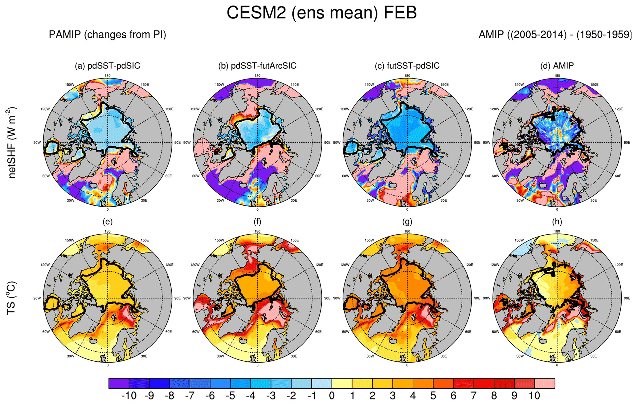
Figure 1Changes in ensemble mean February net surface heat flux (netSHF; a–d) and surface temperatures (TS; e–h) for CESM2 PAMIP (a–c, e–g) and AMIP (d, h). PAMIP differences are from an 1850 pre-industrial control run where both SSTs (sea surface temperatures) and SICs are specified at 1850 levels. Differences from the pre-industrial (PI) control run are shown for PAMIP experiments with present-day SSTs and SICs (pdSST-pdSIC; a, e), present-day SSTs and future SICs (pdSST-futArcSIC; b, f), and future SSTs and SICs (futSST-futArcSIC; c, g). AMIP simulations are from a 10-member ensemble, and differences shown are the ensemble mean of the final decade (2005–2014) minus the first decade (1950–1959) of the simulations. The 98 % SIC contour is shown in black.
Table 1Conductive heat fluxes (Fcond) calculated with Eq. (2) for example sea ice thicknesses (SIT), snow thicknesses (hs), and temperature gradients (ΔT).
2.3 Analysis
We are interested in wintertime Arctic heat fluxes during a period when wintertime central Arctic SICs remain relatively high and changing sea ice and snow thickness will play a dominant role in changing surface fluxes. Thus, we focus initially on 1950–2070 and on the month of February to explore in detail relationships between conductive heat fluxes, snow and sea ice thicknesses, and thickness distributions. Time series presented are area averages over the Arctic Ocean (68–90∘ N from 100–243∘ E and 80–90∘ N elsewhere – see inset in Fig. 2b), thereby reducing the influence of changes in winter sea ice concentrations (SIC) that are seen in the simulations during this time period in the neighboring regions. Changes in conductive heat fluxes due to thinning sea ice dominate the surface heat budget until the sea ice thins enough to subsequently start retreating, exposing open ocean. To highlight this contrast between ice-covered regions and time periods and those with increasing open-water areas, we also show time series from the Kara and Barents seas (see inset in Fig. 5) and some results from October, when SICs are already changing rapidly at the beginning of the 21st century. Our regional definitions are those used by the National Snow & Ice Data Center (https://nsidc.org/, last access: 7 April 2022) and discussed in Cavalieri and Parkinson (2008; 2012) and Parkinson et al. (1999).
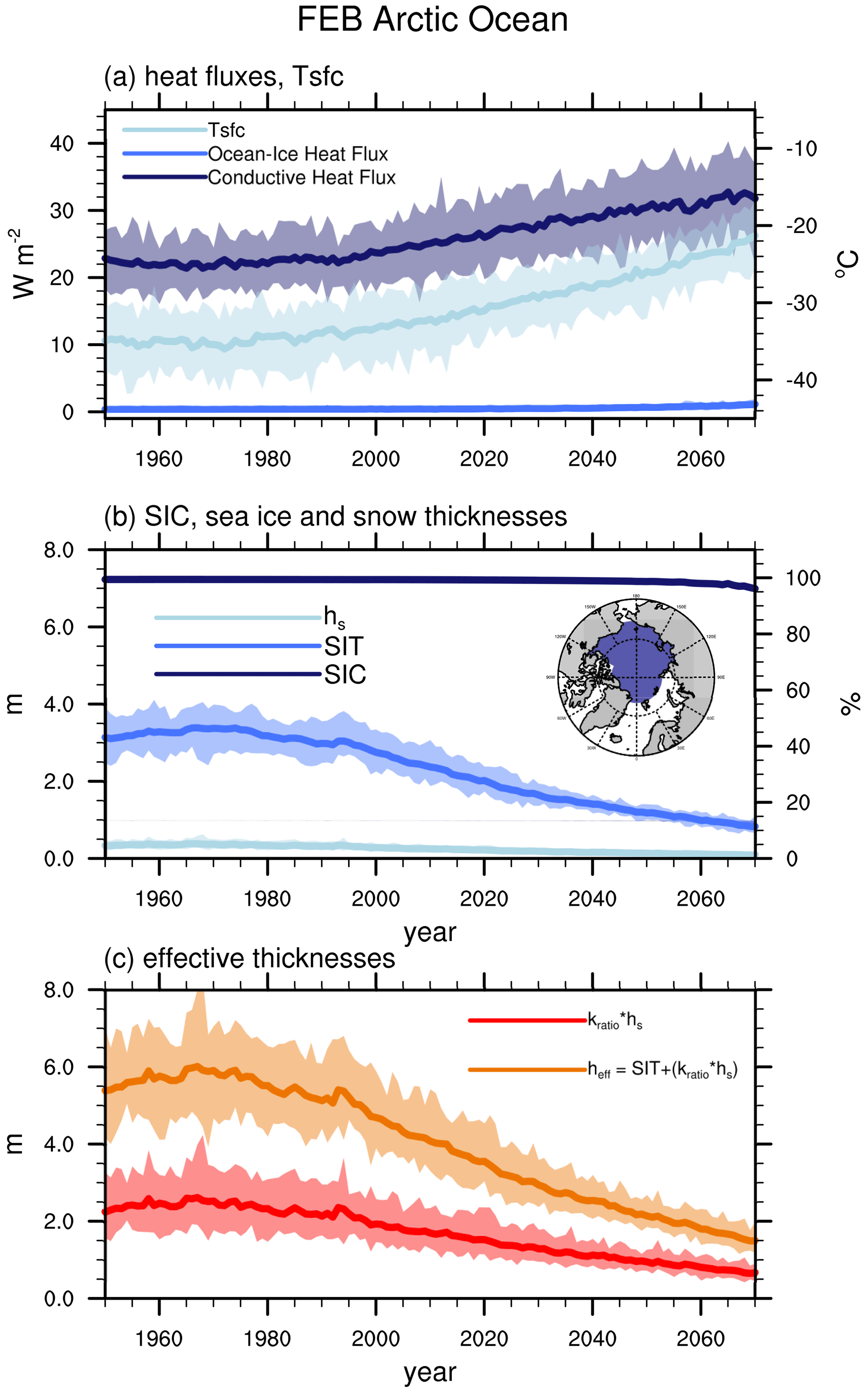
Figure 2CESM1-LE February area-averaged Arctic Ocean (a) surface temperatures, turbulent ocean–sea ice heat fluxes, and conductive heat fluxes (Tsfc); (b) SIC, SIT, and snow thicknesses (hs); and (c) effective snow thickness (Kratio⋅hs) and effective total thicknesses (heff). Ensemble means are shown as solid lines; ensemble ranges are opaque polygons. Arctic Ocean region is shown in the map insert in the middle panel.
We then explore the relative and changing importance of sea ice conductive heat fluxes to the total surface heat fluxes in a warming world in the cold season (October through March) in the 21st century. In the high-latitude Arctic winter, when there is no solar radiation and the surface air temperature is well below the freezing point, the net surface heat flux over the sea ice (total surface short- and longwave radiation and sensible and latent heat fluxes) is balanced by the conductive heat flux through the ice and snow. In regions not 100 % covered by sea ice, there will also be heat flux from the ocean to the atmosphere. The relative contributions of heat fluxes from ocean and sea ice areas will change both as ice and snow thin and as sea ice concentrations decrease. We ask how these relative contributions change in winter months as the projected climate warms and compare ice-covered regions with two regions (Barents Sea and Kara Sea) that are experiencing significant wintertime sea ice concentration losses from 2010–2070.
We also assess the role of sub-grid-cell sea ice thickness distributions in simulated conductive heat fluxes. Model output of conductive heat flux is available on a grid-cell level and is computed as the area-weighted average of the sub-grid-cell conductive heat fluxes. This explicitly accounts for changing ice and snow thicknesses, surface temperatures, and areal concentrations for the different ice thickness categories. Although sub-grid-cell conductive heat flux information that would enable us to directly relate changes in the sub-grid-cell ITD to the net flux was not saved and is not available, sub-grid-cell ice and snow thicknesses are available. Comparisons between the model net grid-cell conductive heat fluxes and those calculated using the sub-grid-cell ice and snow thicknesses, the grid-cell surface temperatures, and the zero-layer model demonstrate that the zero-layer model gives a good approximation for this analysis (Supplement). We then compare the model conductive heat fluxes which account for the sub-grid-scale ice thickness distribution (CESM1-LE) with those calculated from the grid-cell mean SIT and snow thicknesses using the zero-layer model (MNthick) to investigate the influence of snow and sea ice heterogeneity on conductive heat flux calculations.
3.1 Sea ice and snow thicknesses
Over the Arctic Ocean, simulated February surface temperatures and conductive heat fluxes, which are equivalent to the ice–atmosphere heat exchange, increase by ∼8 ∘C and 9 W m−2 between the late 20th century and 2070 in the CESM1-LE (Fig. 2a). The turbulent heat flux exchange between the ocean and the sea ice increases during this time as well – however by less than 1 W m−2 and therefore is not a dominant contribution to the increased net surface heat exchange. Increases in conductive heat flux are driven by decreases in sea ice and snow thickness, since the increase in surface temperatures alone would result in a decrease in conductive heat fluxes (Eq. 2). During this time, sea ice concentrations in the Arctic Ocean remain high, yet sea ice and snow thin dramatically (Fig. 2b), with a mean total effective thickness (heff) decreasing from a peak near 6 m in the 1970s to 1.5 m by 2070 (Fig. 2c). Snow thicknesses averaged over the Arctic Ocean region are typically less than 0.5 m thick – much thinner than sea ice – however snow, as well as changes in snow, makes a significant contribution to both the total effective thickness and the changes in total effective thickness, due to the much larger insulating capacity of snow (Fig. 2c). The decreasing wintertime snow depths over the 21st century in the CESM1-LE are due primarily to sea ice forming later in the fall, which in turns leads to a later start of the accumulation of snow on the sea ice (e.g., Webster et al., 2014; 2018; 2020). This mechanism has also been found in projections of snow on sea ice (Hezel et al., 2012) and in observations (Webster et al., 2014; 2018). In addition, as the temperatures warm, the rain/snow seasons increase/decrease (e.g., Webster et al., 2020).
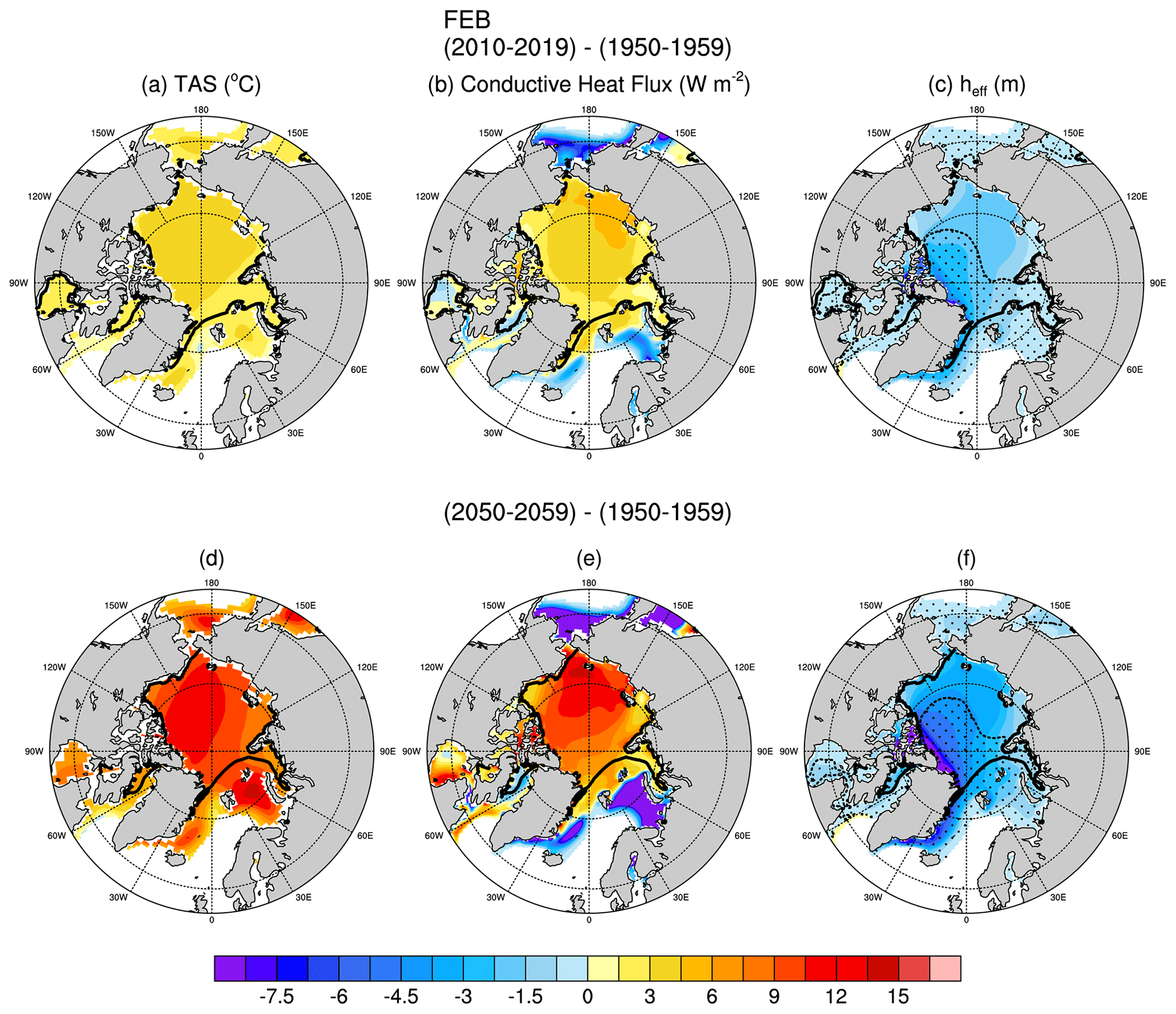
Figure 3February decadal mean changes (from 1950–1959) in surface temperatures (a, d), conductive heat fluxes (b, e), and effective sea ice + snow thickness (heff; e, f) for the 2010s (a, b, c) and 2050s (d, e, f). The 98 % SIC for each decade is shown by the thick black contour. Stippled areas in the effective thickness (heff) change figures (c, f) indicate regions where changes in effective snow thickness (Kratio⋅hs) account for 40 % or more of the changes in the total effective thickness (heff = SIT + Kratio⋅hs).
Conductive heat fluxes increase first over the East Siberian and Chukchi seas (Fig. 3). By the 2050s, increases in conductive heat fluxes of 9–12 W m−2 are seen not only in the Chukchi and East Siberian seas but also extending into the Beaufort Sea and the central Arctic Ocean. Surface temperature increases likewise show the earliest and greatest increases on the Pacific side of the Arctic Ocean. However, by the 2050s the areas of greatest warming (>10 ∘C) are present over comparatively larger sections of the Arctic Ocean and Beaufort Sea and extend as far as northern Greenland. Sea ice concentrations remain above 95 % in the Arctic Ocean even by the 2050s. As such, changes in heat fluxes from the relatively warmer surface to the colder atmosphere primarily result from thinning sea ice and snow rather than increases in open water (see Sect. 3.2). Changes in sea ice thicknesses in the CESM1-LE tend to be largest from the Canadian Archipelago, across the central Arctic Ocean, and onto the East Siberian Sea (Supplement), whereas changes in snow thickness are greatest near the Canadian Archipelago and northern and eastern Greenland. Changes in both sea ice and snow thicknesses are important contributors to the changes in effective thickness (Fig. 3). Although snow depth changes are small compared to changes in SIT, they contribute 40 % or more to the changes in effective thicknesses from the central Arctic Ocean to the Canadian Archipelago, to Greenland, and into the Atlantic sector of the Arctic Ocean (Fig. 3 and Supplement). It is important to note that changes in conductive heat fluxes during this time are mitigated by changes in surface temperatures: the roughly 13 ∘C surface warming over this period would lead to a ∼5 W m−2 decrease in conductive heat flux if the sea ice and snow did not thin (and as they do in the AMIP and PAMIP atmosphere only runs when SITs are held constant – e.g., Fig. 1).
3.2 Relative contributions of conductive heat flux changes to total surface heat flux changes in a warming climate
Changes in conductive heat fluxes due to thinning sea ice dominate the surface heat budget until the sea ice thins enough to subsequently start retreating, whereupon the surface heat flux quickly becomes dominated by fluxes from exposed open water (Figs. 4 and 5). Ensemble mean February net surface heat fluxes over the Arctic ocean increase modestly from the 1950s to the 2010s (∼3–6 W m−2), then by ∼10–18 W m−2 by the 2050s. Arctic Ocean SICs remain above 98 % – increases in surface heat flux are primarily due to changes in snow and ice thicknesses, with open-water areas contributing less than 10 %–25 % to the net surface heat flux budget. In contrast, outside of the ice-covered areas, increases in surface heat fluxes are larger than 25 W m−2 and predominantly due to fluxes from open water. In February, these areas expand from the Sea of Okhotsk and the Bering, Kara, and Barents seas in the 2010s to include most of the Arctic Ocean by the end of the 21st century. Rates of surface temperature warming reflect this as well – with the highest February Arctic amplifications occurring initially over the Chukchi and East Siberian seas, where sea ice is thinning; over the Barents and Kara seas by the 2050s; and finally over large sections of the Arctic Ocean as SICs fall by the 2090s (Fig. 4). These patterns of relative contributions of sea ice and ocean to the net surface heat fluxes, as well as corresponding rates of AA, are also seen in the fall (October; Supplement), when observed AAs are highest (e.g., Chung et al., 2021) and underscore the transient and seasonal nature of AA which may increase in regions experiencing sea ice loss before decreasing again after becoming ice free (e.g., Holland and Landrum, 2021). Regionally averaged time series show how contributions from open ocean water to the net surface heat fluxes tend to be greater than those from ice once SICs fall below ∼90 % – highlighting how changes in surface heat fluxes will be dominated by those over sea ice (due to thinning sea ice and snow) until sea ice itself starts retreating (Fig. 5). Variability in heat fluxes from the ocean tends to be very high compared to those from sea ice, particularly in the Barents and Kara seas.
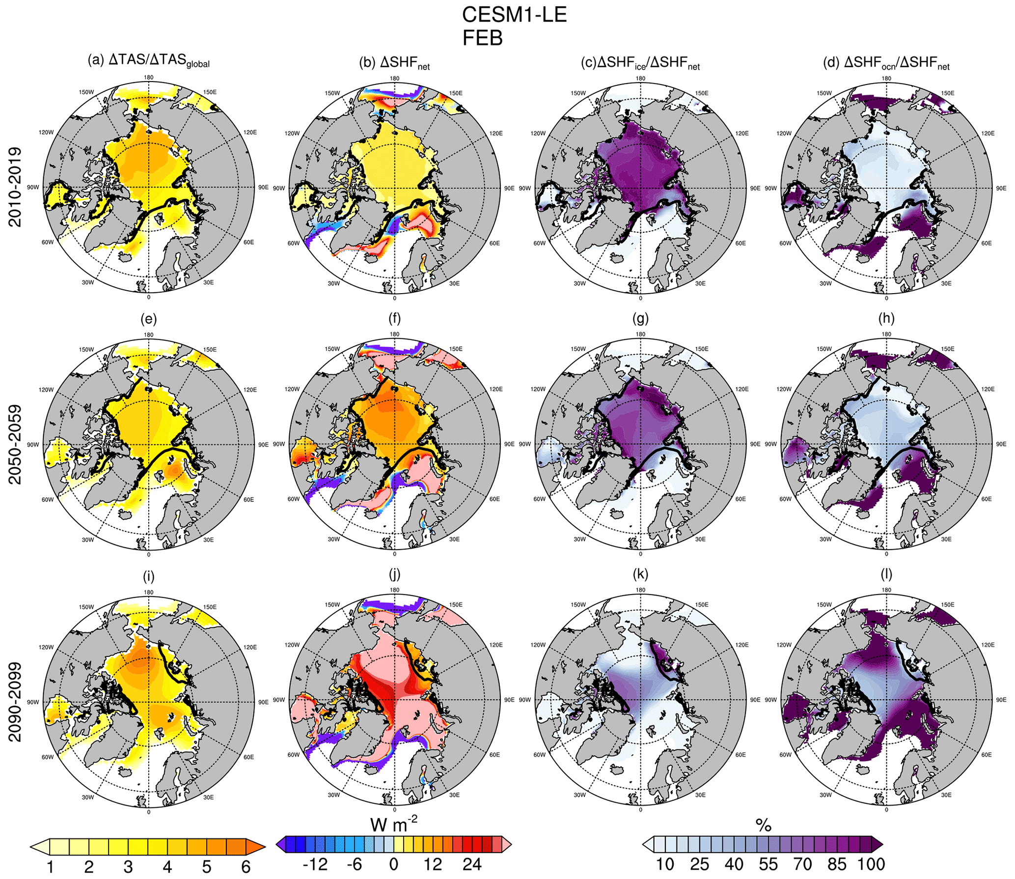
Figure 4February decadal mean changes (1950–1959) in Arctic amplification (Δ TAS/ΔTASglobal, where TAS is the near-surface air temperature; a, e, i), net surface heat fluxes (b, f, j), sea ice contribution to surface heat fluxes (c, g, k), and ocean contributions to surface heat fluxes (SHFs) (d, h, l) for the 2010s (a, b, c, d), the 2050s (e, f, g, h), and the 2090s (i, j, k, l). The 98 % SIC for each decade is shown by the thick black contour.
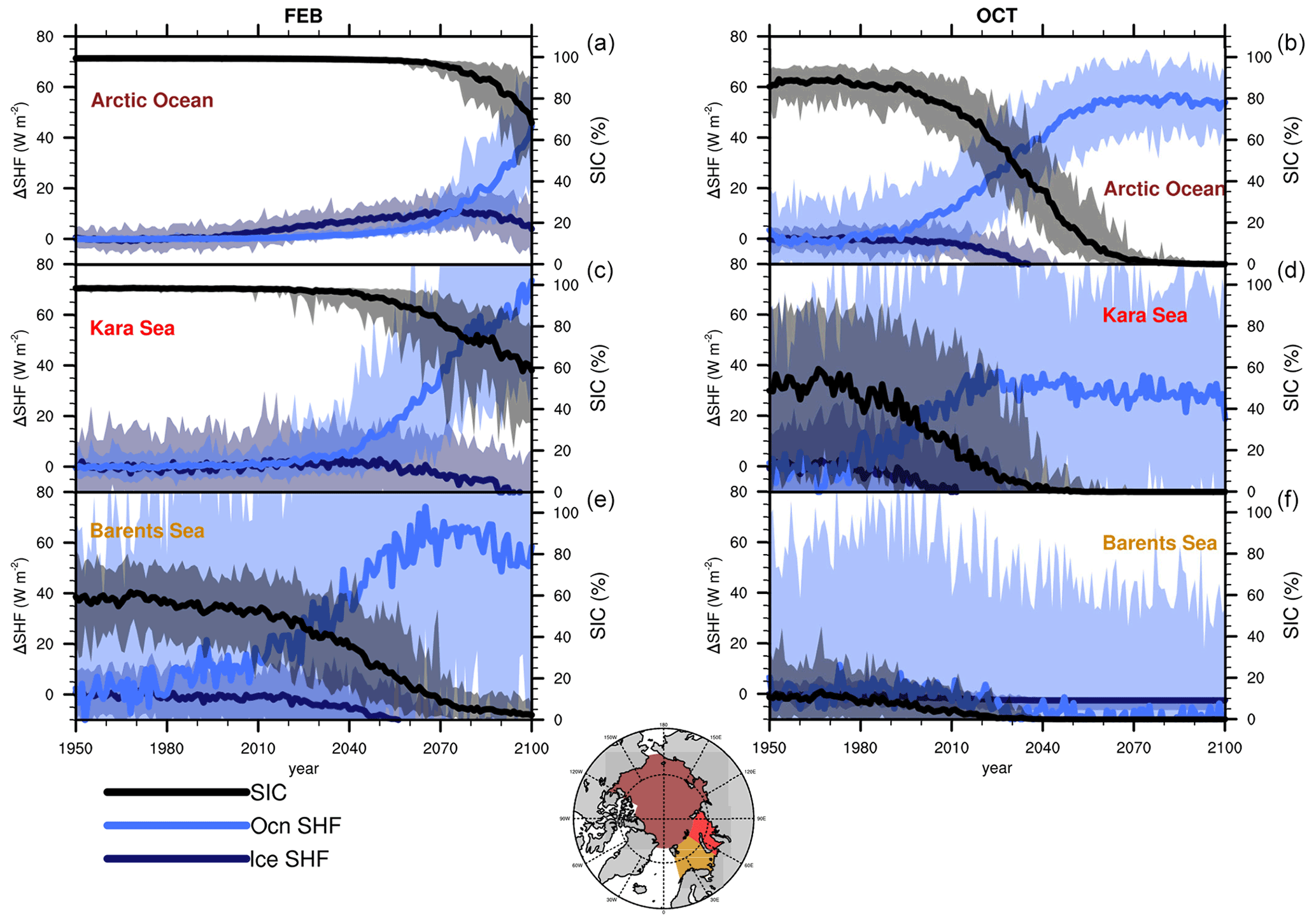
Figure 5CESM1-LE area-averaged anomalies (from the 1950–1959 ensemble mean) for sea ice and ocean contributions to net surface heat fluxes (left axis) and sea ice concentrations (right axis) for February (a, c, e) and October (b, d, f) for the Arctic Ocean (a, b), Kara Sea (c, d), and Barents Sea (e, f). Ensemble means are shown as solid lines; ensemble ranges are opaque polygons. Geographic areas are shown in the inset at the bottom.
3.3 Sea ice and snow thickness distributions
Given the nonlinear response of the conductive heat flux to ice and snow thickness, the changing distribution of ice at the sub-grid-cell level may play an important role. We investigate the influence of thickness distributions on conductive heat fluxes by calculating conductive heat fluxes using the Semtner zero-layer model, daily mean sea ice, and snow thicknesses over the ice-covered areas in each grid cell along with daily grid-cell average surface temperatures (MNthick) and then averaging over the month of February. Relative to an estimate of the fluxes computed by the full model (CESM1-LE), the MNthick conductive heat fluxes underestimate heat fluxes throughout the Arctic Ocean (Fig. 6a and Supplement). Ensemble mean Arctic Ocean average conductive heat flux is underestimated by ∼6–9 W m−2 using MNthick (Fig. 6). This highlights the importance of resolving thin ice and snow within the sub-grid-scale ice thickness distribution.
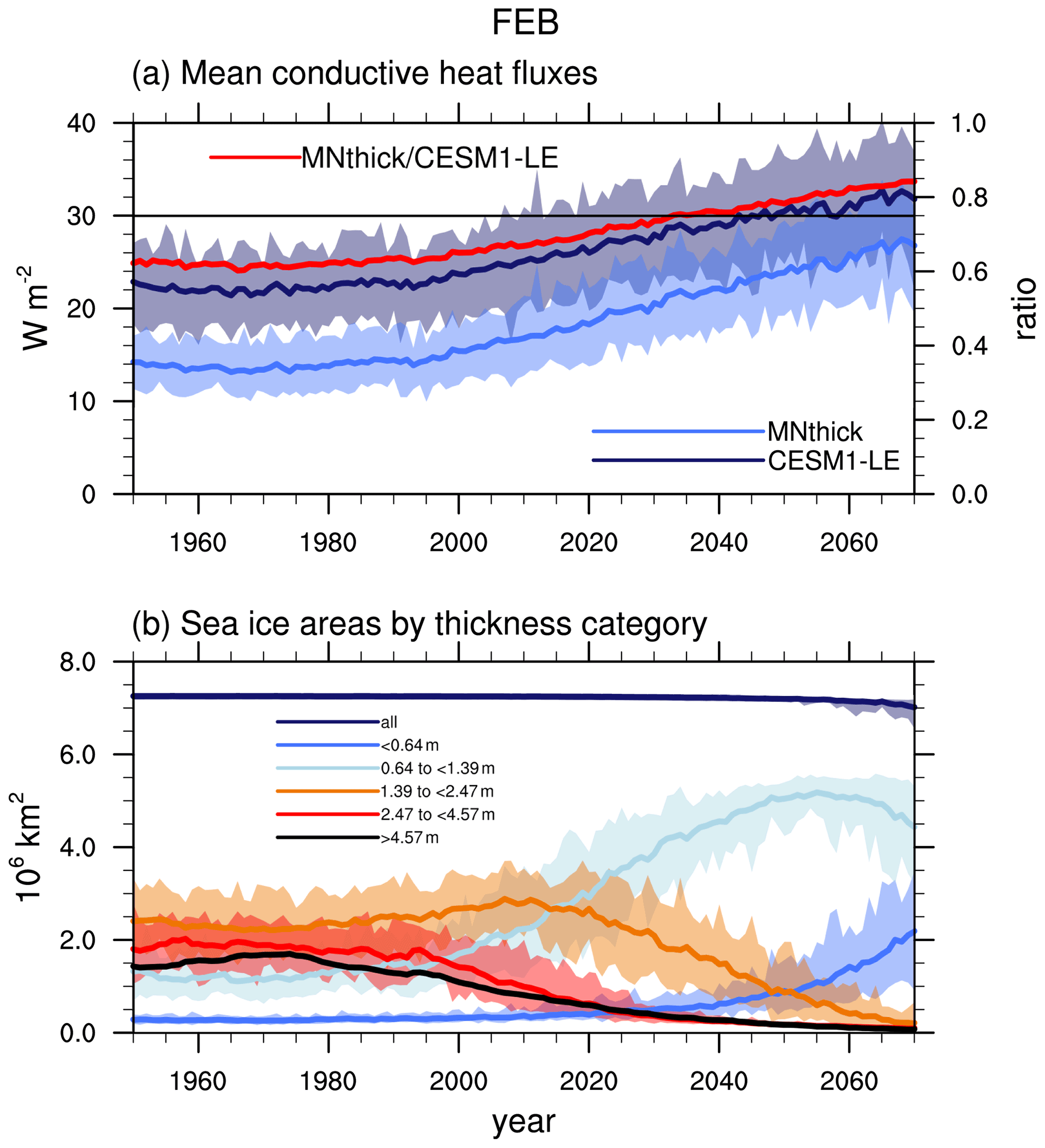
Figure 6CESM1-LE February area-averaged Arctic Ocean (a) mean conductive heat fluxes from the model output (CESM1-LE; dark blue) and calculated from mean ice and snow thicknesses (MNthick; light blue) and the ratio of MNthick to CESM1-LE (red) and (b) sea ice areas by thickness category as well as total sea ice area (dark blue). Ensemble means are shown as solid lines; ensemble ranges are opaque polygons. The solid black line in the top panel indicates a MNthick : CESM1-LE conductive heat flux ratio of 0.75 for reference.
Differences between these wintertime conductive heat fluxes throughout the Arctic basin are larger in the beginning of the 21st century (by ∼35 %) when considerable thick ice is present. Discrepancies between MNthick conductive heat flux estimates and the CESM1-LE are reduced by the 2070s (to ∼16 %) when almost all the February sea ice in the Arctic Ocean has thinned considerably to less than 1 m over the Arctic Ocean and the ITD lies within the two thinnest sea ice categories (Fig. 6b). Although grid-cell average thicknesses lead to an underestimation of mean conductive heat fluxes, they result in an overestimation in the changes in conductive heat fluxes (by ∼36 % by 2070; Fig. 6a) and thus influence feedbacks in the warming climate.
This analysis has important implications for atmosphere-only simulations and reanalysis products that require specified sea ice concentrations, sea ice thicknesses, and snow depths for boundary conditions. These simulations typically prescribe changes in sea ice concentration but neglect changes in ice and snow thickness. The sea ice concentration changes lead to large changes in surface albedos and direct ocean–atmosphere heat fluxes as more ocean water is exposed to the atmosphere. However, by neglecting changes in ice and snow thickness, the changing insulating effect of sea ice is missing. As the climate warms, changing winter Arctic surface heat fluxes will be dominated by this insulating effect and resulting changes in conductive heat fluxes until the SICs decrease enough such that direct ocean–atmosphere heat fluxes become more important. In the CESM1-LE, with changing sub-grid-scale ice and snow thicknesses, conductive heat fluxes contribute over half of the December–March surface heat fluxes until 2050–2070 (not shown). Atmosphere-only simulations that consider only changes in sea ice concentrations and ignore changes in sea ice and snow thicknesses simulate decreasing conductive heat fluxes – the winter atmosphere in high-SIC regions gains less heat from the surface under climate warming. When changing ice thicknesses and snow depths are accounted for, conductive heat fluxes increase, and the atmosphere gains more heat from the surface. In the CESM1-LE, Arctic basin conductive heat flux increases by ∼8–10 W m−2 from 2000 to 2070 as winter SICs remain above 95 %.
Sea ice and snow exhibit high spatial heterogeneity, and climate models often account for this through the inclusion of a sub-grid-scale ice thickness distribution within their sea ice treatment. This heterogeneity of both sea ice and snow fields impacts conductive heat fluxes and thus the projected changes in the net surface heat flux. Whereas most climate models participating in the most recent Coupled Model Intercomparison Project (CMIP6) employ sea ice models with sub-grid-scale sea ice thickness distributions (e.g., Keen et al., 2021), atmosphere-only simulations (for example, AMIP and PAMIP style simulations) calculate sea ice thermodynamics over only grid-cell mean sea ice and snow thicknesses. This will underestimate mean wintertime conductive heat fluxes and, in the PAMIP simulations that allow for thickness to change, will overestimate changes in conductive heat fluxes as the ice thins. These differences can be significant – in the CESM1-LE mean conductive heat fluxes calculated using grid-cell mean thicknesses lead to an underestimation of ∼16 %–35 % in mean values and an overestimation of up to ∼36 % in the changes in conductive heat fluxes in the wintertime Arctic basin where SICs remain above 95 %.
Snow is a much more effective insulator than sea ice and plays important roles in sea ice mass budgets and climate feedbacks. Snow distributions on sea ice remain, however, an area of large uncertainty and potential errors in both climate model simulations and reanalysis products. PAMIP protocols and reanalysis products use either very simplified snow (accumulations only through precipitation) or nonexistent snow routines, with resultant flux estimates that show large wintertime heat flux biases when compared to the recent Norwegian Young Sea Ice campaign (N-ICE2015) observations (e.g., Bromwich et al., 2018; Graham et al., 2017). Yet snow – highly reflective and highly insulating – plays an outsized role in Arctic heat budgets. Reanalysis products show consistent warm bias in winter sea ice surface temperatures (e.g., Batrak and Müller, 2019; Graham et al., 2017; 2019; Jakobson et al., 2012; Lindsay et al., 2014), with recent work attributing this to misrepresentation of snow on sea ice (Batrak and Müller, 2019).
Snow and sea ice thicknesses and distributions in the CESM1-LE are roughly equally important contributors to wintertime conductive heat fluxes. Snow depth distributions in the CESM1-LE show similar patterns compared to observations across the Arctic Basin, although simulated snow depths tend to be more evenly distributed and thicker than observed (Webster et al., 2020). Snow thicknesses in the most recent version of CESM – the CESM2 – tend to be underestimated and have low variability compared to observations. These differences between simulations are due largely to differences in precipitation and the mean sea ice state in these two models (Webster et al., 2020). Discrepancies between simulations and observations, however, are not well understood and suggest that future collaborative work to test and improve snow distributions in the modeling environment would be important for increasing our understanding of Arctic climate and predicting snow impacts in a warming climate.
The results presented here are from a large ensemble of simulations from one climate model. Recent contributions from multiple modeling centers to the CMIP6 suggest that the sea ice components in climate models are responding consistently to external forcing (e.g., Keen et al., 2021), and our results are not expected to change fundamentally with different climate models, although the timing may differ based on the mean ice state. In the CESM1-LE SICs remain above 98 % in the high-latitude Arctic Ocean until the end of the 21st century, and this timing will differ depending on the initial mean ice state and transient response in a given model. For example, the most recent version of the model, the CESM2, includes many changes to all model components, and Arctic sea ice in the CESM2 tends to be thinner, less extensive, and less persistent than in the CESM1-LE (DeRepentigny et al., 2020).
These results highlight the transient nature of the influences of SIT, snow thicknesses, and their distributions on Arctic wintertime surface heat budgets. The thermodynamics of sea ice are dependent on the mean ice state (e.g., Massonnet et al., 2018) – and this has important implications for not only sea ice evolution in a changing world but also surface heat fluxes in ice-covered areas. Models with a relatively thin sea ice mean state will have higher errors in changes in surface heat fluxes depending on whether they use grid-cell mean SITs or heterogeneous fields. Sea ice and snow on sea ice are important components of polar climate thermodynamics, and their dynamic and heterogeneous nature – although complicated – plays important roles in surface heat budgets.
All analysis and figures were completed using the NCAR (National Center for Atmospheric Research) Command Language (NCAR Command Language v.6.6.2; NCAR, 2019, https://doi.org/10.5065/D6WD3XH5). The scripts used to perform the analysis and generate the figures in this paper are available on GitHub (https://github/llandrum/Cryosphere_SeaIce_Snow_Thicknesses_ArcticHeatFlux, last access: 7 April 2022) and archived in Zenodo (https://doi.org/10.5281/zenodo.6336145; Landrum, 2021). The CESM-LE data are freely available from the following link: http://www.cesm.ucar.edu/projects/community-projects/LENS/ (last access: 7 April 2020, Deser and Kay, 2020; Kay et al., 2015). The PAMIP data with CAM6 (Community Atmosphere Model version 6) are accessible on the Earth System Grid Federation website (https://esgf-node.llnl.gov/search/cmip6/, last access: 6 April 2022, Danabasoglu, 2019a, b, c).
The supplement related to this article is available online at: https://doi.org/10.5194/tc-16-1483-2022-supplement.
LLL and MMH formulated the research goals and questions. LLL made the figures and performed the analysis with input from MMH. LLL prepared the manuscript with contributions from MMH.
The contact author has declared that neither they nor their co-authors have any competing interests.
Publisher's note: Copernicus Publications remains neutral with regard to jurisdictional claims in published maps and institutional affiliations.
We acknowledge the CESM Large Ensemble Community Project and supercomputing resources (https://doi.org/10.5065/D6RX99HX) provided by the Climate Simulation Laboratory at NCAR's Computational and Information Systems Laboratory, sponsored by the National Science Foundation and other agencies.
We thank Alice DuVivier for providing the daily CESM1-TS data so that we could compare zero-layer to multi-layer model estimates of conductive heat fluxes.
This research has been supported by the National Science Foundation Office of Polar Programs (grant no. NSF-OPP 1724748).
This paper was edited by Tobias Sauter and reviewed by two anonymous referees.
Batrak, Y. and Müller, M.: On the warm bias in atmospheric reanalyses induced by the missing snow over Arctic sea-ice, Nat. Commun., 10, 4170, https://doi.org/10.1038/s41467-019-11975-3, 2019.
Bitz, C. M. and Lipscomb, W. H.: An energy-conserving thermodynamic sea ice model for climate study, J. Geophys. Res.-Oceans, 104, 15669–15677, https://doi.org/10.1029/1999JC900100, 1999.
Bromwich, D. A., Wilson, A. B., Bai, L., Liu, Z., Barlage, M., Shih, C.-F., Maldonado, S., Hines, K. M., Wang, S.-H., Woollen, J., Kuo, B., Lin, H.-C., Wee, T.-K., Serreze, M. C., and Walsh, J. E.: The Arctic System Reanalysis, version 2, Bull. Amer. Meteor. Soc., 99, 805–828, https://doi.org/10.1175/BAMS-D-16-0215.1, 2018.
Cavalieri, D. J. and Parkinson, C. L.: Antarctic Sea Ice Variability and Trends, 1979–2006, J. Geophys. Res., 113, C07004, https://doi.org/10.1029/2007JC004564, 2008.
Cavalieri, D. J. and Parkinson, C. L.: Arctic sea ice variability and trends, 1979–2010, The Cryosphere, 6, 881–889, https://doi.org/10.5194/tc-6-881-2012, 2012.
Chung, E., Ha, K., Timmermann, A., Stuecker, M., Bodai, T., and Lee, S.: Cold-season Arctic Amplification driven by Arctic Ocean-mediated seasonal energy transfer, Earths Future, 9, e2020EF001898, https://doi.org/10.1029/2020EF001898, 2021.
Dai, A., Luo, D., Song, M., and Liu, J.: Arctic amplification is caused by sea-ice loss under increasing CO2, Nat. Commun., 10, 121, https://doi.org/10.1038/s41467-018-07954-9, 2019.
Danabasoglu, G.: NCAR CESM2 model output prepared for CMIP6 PAMIP pdSST-pdSIC, Version 20210323, Earth System Grid Federation, https://doi.org/10.22033/ESGF/CMIP6.7696, 2019a.
Danabasoglu, G.: NCAR CESM2 model output prepared for CMIP6 PAMIP futSST-pdSIC, Version 20210323, Earth System Grid Federation, https://doi.org/10.22033/ESGF/CMIP6.7592, 2019b.
Danabasoglu, G.: NCAR CESM2 model output prepared for CMIP6 PAMIP pdSST-futArcSIC, Version 20210323, Earth System Grid Federation, https://doi.org/10.22033/ESGF/CMIP6.7692, 2019c.
DeRepentigny, P., Jahn, A., Holland, M. M., and Smith, A.: Arctic sea ice in two configurations of the Community Earth System Model Version 2 (CESM2) during the 20th and 21st centuries, J. Geophys. Res.-Oceans, https://doi.org/10.1029/2020JC016133, 2020.
Deser, C. and Kay, J. E.: CESM Large Ensemble Community Project [data set], http://www.cesm.ucar.edu/projects/community-projects/LENS/, last access: 7 April, 2020.
Feldl, N., Po-Chedley, S., Singh, H. K. A., Hay, S., and Kushner, P. J.: Sea ice and atmospheric circulation shape the high-latitude lapse rate feedback, Nature Partner Jounals, Clim. Atmos. Sci., 3, 41, doi.org/10.1038/s41612-020-00146-7, 2020.
Gerdes, R.: Atmospheric response to changes in Arctic sea ice thickness, Geophys. Res. Lett., 33, L18709, https://doi.org/10.1029/2006GL027146, 2006.
Graham, R. M., Rinke, A., Cohen, L., Hudson, S. R., Von Walden, P., Granskog, M. A., Dorn, W., Kayser, M., Maturilli, M.: A comparison of the two Arctic atmospheric winter states observed during N-ICE2015 and SHEBA, J. Geophys. Res.-Atmos., 122, 5716–5737, https://doi.org/10.1002/2016JD025475, 2017.
Graham, R. M., Cohen, L., Ritzhaupt, N., Segger, B., Graverson, R. R., Rinke, A., Walden, V. P., Granskog, M. A., and Hudson, S. R.: Evaluation of Six Atmospheric Reanalysis over Arctic Sea Ice from Winter to Early Summer, J. Climate, 32, 4121–4143, https://doi.org/10.1175/JCLI-D-18-0643.1, 2019.
Graversen, R. G. and Wang, M.: Polar amplification in a coupled climate model with locked albedo, Clim. Dynam., 33, 629–643, 2009.
Hall, A.: The role of surface albedo feedback in climate, J. Climate, 17, 1550–1568, 2004.
Hezel, P. J., Zhang, X., BItz, C. M., Kelly, B. P., and Massonnet, F.: Projected decline in spring snow depth on Arctic sea ice caused by progressively later autumn open ocean freeze-up this century, Geophys. Res. Lett., 39, L17505, https://doi.org/10.1029/2012GL052794, 2012.
Holland, M. M., Bitz, C. M., Hunke, E. C., Lipscomb, W. H., and Schramm, J. L.: Influence of the sea ice thickness distribution on polar climate in CCSM3, J. Clim., 19, 2398–2414, 2006.
Holland, M. M. and Landrum, L.: The emergence and transient nature of Arctic amplification in coupled climate models, Front. Earth Sci., 9, 2296–6463, https://doi.org/10.3389/feart.2021.719024, 2021.
Hunke, E., Lipscomb, W., Jones, P., Turner, A., Jeffery, N., and Elliott, S.: CICE, The Los Alamos Sea Ice Model, Computer software, https://www.osti.gov//servlets/purl/1364126. Vers. 00. USDOE, last access: 12 May 2017.
Hurrell, J. W., Hack, J. J., Shea, D., Caron, J. M., and Rosinski, J.: A new sea surface temperature and sea ice boundary dataset for the Community Atmosphere Model, J. Climate, 21, 5145–5153, 2008.
Huwald H., Tremblay, L. B., and Blatter, H.: Reconciling different observational data sets from Surface Heat Budget of the Arctic Ocean (SHEBA) for model validation purposes, J. Geophys. Res. 110, C05009, https://doi.org/10.1029/2003JC002221, 2005.
Jakobson, E., Vihma, T., Palo, T., Jakobson, L., Keernik, H., and Jaagus, J.: Validation of atmospheric reanalysis over the center Arctic Ocean, Geophys. Res. Lett., 39, L10802, https://doi.org/10.1029/2012GL051591, 2012.
Kay, J. E., Deser, C., Phillips, A., Mai, A., Hannay, C., Strand, G., Arblaster, J., Bates, S., Danabasoglu, G., Edwards, J., Holland, M. Kushner, P., Lamarque, J.-F., Lawrence, D., Lindsay, K., Middleton, A., Munoz, E., Neale, R., Oleson, K., Polvani, L., and Vertenstein, M.: The Community Earth System Model (CESM) Large Ensemble Project: a community resource for studying climate change in the presence of internal climate variability, Bull. Am. Meteorol. Soc., 96, 1333–1349, https://doi.org/10.1175/BAMS-D-13-00255.1, data available at: http://www.cesm.ucar.edu/projects/community-projects/LENS/ (last access: 7 April 2020), 2015.
Keen, A., Blockley, E., Bailey, D. A., Boldingh Debernard, J., Bushuk, M., Delhaye, S., Docquier, D., Feltham, D., Massonnet, F., O'Farrell, S., Ponsoni, L., Rodriguez, J. M., Schroeder, D., Swart, N., Toyoda, T., Tsujino, H., Vancoppenolle, M., and Wyser, K.: An inter-comparison of the mass budget of the Arctic sea ice in CMIP6 models, The Cryosphere, 15, 951–982, https://doi.org/10.5194/tc-15-951-2021, 2021.
Krinner, G., Rinke, A., Dethloff, K., and Gorodetskaya, I. V.: Impact of prescribed Arctic sea ice thickness in simulations of the present and future climate, Clim. Dyn., 35, 619–633, https://doi.org/10.1007/s00382-009-0587-7, 2010.
Kumar, A., Perlwitz, J., Eischeid, J., Quan, X., Xu, T., Zhang, T., Hoerling, M., Jha, B., and Wang, W.: Contribution of sea ice loss to Arctic amplification, Geophys. Res. Lett., 37, L21701, https://doi.org/10.1029/2010GL045022, 2010.
Kwok, R.: Arctic sea ice thickness, volume, and multiyear ice coverage: losses and coupled variability (1958–2018), Environ. Res. Lett., 13, 105005, https://doi.org/10.1088/1748-9326/aae3ec, 2018.
Kwok, R. and Rothrock, D. A.: Decline in Arctic sea ice thickness from submarine and ICESat records: 1958–2008, Geophys. Res. Lett., 36, L15501, https://doi.org/10.1029/2009GL039035, 2009.
Labe, Z., Magnusdottir, G., and Stern, H.: Variability of Arctic sea ice thickness using PIOMAS and the CESM large ensemble, J. Climate, 31, 3233–3247, https://10.1175/ JCLI-D-17-0436.1, 2018a.
Labe, Z. M., Peings, Y., and Magnusdottir, G.: Contributions of ice thickness to the atmospheric response from projected Arctic sea ice loss, Geophys. Res. Lett., 45, 5635–5642, https://doi.org/10.1029/2018GL078158, 2018b.
Landrum, L.: Scripts for figures and analysis for “Influences of changing sea ice and snow thicknesses on winter Arctic heat fluxes” in The Cryosphere, Zenodo [code], https://doi.org/10.5281/zenodo.6336145, 2021.
Lang, A., Yang, S. and Kaas, E.: Sea ice thickness and recent Arctic warming, Geophys. Res. Lett., 44, 409–418, https://doi.org/10.1002/2016GL071274, 2017.
Lindsay, R. and Schweiger, A.: Arctic sea ice thickness loss determined using subsurface, aircraft, and satellite observations, The Cryosphere, 9, 269–283, https://doi.org/10.5194/tc-9-269-2015, 2015.
Lindsay, R., Wensnahan, M., Schweiger, A., and Zhang, J.: Evaluation of seven different atmospheric reanalysis products in the Arctic, J. Climate, 27, 2588–2606, https://doi.org/10.1175/JCLI-D-13-00014.1, 2014.
Massonnet, F., Vancoppenolle, M., Goosse, H., Docquier, D., Fichefet, T., and Blanchard-Wrigglesworth, E.: Arctic sea-ice change tied to its mean state through thermodynamic processes, Nat. Clim. Change, 8, 599–603, https://doi.org/10.1038/s41558-018-0204-z, 2018.
Meinshausen, M., Smith, S. J., Calvin, K. Daniel, J. S., Kainuma, M. L. T., Lamarque, J.-F., Matsumoto, K., Montzka, S. A., Raper, S. C. B., Riahi, K., Thomson, A., Velders, G. J. M., and van Vuuren, D. P. P.: The RCP greenhouse gas concentrations and their extensions from 1765 to 2300, Clim. Change, 109, 213, https://doi.org/10.1007/s10584-011-0156-z, 2011.
NCAR: The NCAR Command Language (NCL), Version 6.6.2, NCAR [code], Boulder, Colorado, UCAR/NCAR/CISL/TDD, https://doi.org/10.5065/D6WD3XH5, 2019.
Parkinson, C. L., Cavalieri, D. J., Gloersen, P., Zwally, H. J., and Comiso, J. C.: Arctic sea ice extents, areas, and trends, 1978–1996, J. Geophys. Res., 104, 20837–20856, https://doi.org/10.1029/1999JC900082, 1999.
Peings, Y. and G. Magnusdottir, G.: Response of the wintertime Northern Hemisphere atmospheric circulation to current and projected Arctic sea ice decline: A numerical study with CAM5, J. Climate, 27, 244–264 https://doi.org/10.1175/JCLI-D-13-00272.1, 2014.
Petty, A. A., Holland, M. M., Bailey, D. A., and Kurtz, N. T.: Warm Arctic, increased winter sea ice growth?, Geophys. Res. Lett., 45, 12922–12930, https://doi.org/10.1029/2018GL079223, 2018.
Pithan, F. and Mauritsen, T.: Arctic amplification dominated by temperature feedbacks in contemporary climate models, Nat. Geosci., 7, 181–184, 2014.
Screen, J. A., Simmonds, I., Deser, C., and Tomas, R.: The atmospheric response to three decades of observed Arctic sea ice loss, J. Climate, 26, 1230–1248, https://doi.org/10.1175/JCLI-D-12-00063.1, 2013.
Semtner, A. J.: A Model for the Thermodynamic Growth of Sea Ice in Numerical Investigations of Climate, J. Phys. Oceanogr. 6, 379–389, 1976.
Serreze, M. C. and Barry, R. G.: Processes and impacts of Arctic amplification: A research synthesis, Global Planet. Change, 77, 85–96, https://doi.org/10.1016/j.gloplacha.2011.03.004, 2011.
Simpson, I. R., Bacmeister, J., Neale, R. B., Hannay, C., Gettelman, A., Garcia, R. R., and coauthors: An evaluation of the large-scale atmospheric circulation and its variability in CESM2 and other CMIP models, J. Geophys. Res.-Atmos., 125, e2020JD032835, https://doi.org/10.1029/2020JD032835, 2020.
Smith, D. M., Screen, J. A., Deser, C., Cohen, J., Fyfe, J. C., García-Serrano, J., Jung, T., Kattsov, V., Matei, D., Msadek, R., Peings, Y., Sigmond, M., Ukita, J., Yoon, J.-H., and Zhang, X.: The Polar Amplification Model Intercomparison Project (PAMIP) contribution to CMIP6: investigating the causes and consequences of polar amplification, Geosci. Model Dev., 12, 1139–1164, https://doi.org/10.5194/gmd-12-1139-2019, 2019.
Sun, L., Deser, C., and Tomas, R. A.: Mechanisms of stratospheric and tropospheric circulation response to projected Arctic sea ice loss, J. Climate, 28, 7824–7845, https://doi.org/10.1175/JCLI-D-15-0169.1, 2015.
Sun, L., Allured, D., Hoerling, M., Smith, L., Perlwitz, J., Murray, D., and Eischeid, J.: Drivers of 2016 record Arctic warmth assessed using climate simulations subjected to Factual and Counterfactual forcing, Weather and Climate Extremes, 19, 1-9, https://doi.org/10.1016/j.wace.2017.11.001, 2018.
Sun, L., Deser, C., Simpson I., and Sigmond, M.: Uncertainty in the winter tropospheric response to Arctic Sea ice loss: the role of stratospheric polar vortex internal variability, J. Climate, 35, 1–58, https://doi.org/10.1175/JCLI-D-21-0543.1, 2022.
Thorndike, A. S., Rothrock, D., Maykut, G., and Colony, R.: The thickness distribution of sea ice, J. Geophys. Res., 80, 4501–4513, 1975.
Vavrus, S.: The impact of cloud feedbacks on Arctic climate under greenhouse forcing, J. Climate, 17, 603–615, 2004.
Wang, C., Graham, R. M., Wang, K., Gerland, S., and Granskog, M. A.: Comparison of ERA5 and ERA-Interim near-surface air temperature, snowfall and precipitation over Arctic sea ice: effects on sea ice thermodynamics and evolution, The Cryosphere, 13, 1661–1679, https://doi.org/10.5194/tc-13-1661-2019, 2019.
Webster, M., Gerland, S., Holland, M., Hunke, E., Kwok, R., Lecomte, O., Massom, R., Perovich, D., and Sturm, M.: Snow in the changing sea-ice systems, Nat. Clim. Change, 8, 946–953, https://doi.org/10.1038/s41558-018-0286-7, 2018.
Webster, M. A., Rigor, I. G., Nghiem, S. V., Kurtz, N. T., Farrell, S. L., Perovich, D. K., and Sturm, M.: Interdecadal changes in snow depth on Arctic sea ice, J. Geophys. Res.-Oceans, 119, 5395–5406, 2014.
Webster, M. A., DuVivier, A. K., Holland, M. M., and Bailey, D. A.: Snow on Arctic Sea Ice in a Warming Climate as Simulated in CESM, J. Geophys. Res.-Oceans, 125, e2020JC016308, https://doi.org/10.1029/2020JC016308, 2020.
Zhang, J. and Rothrock, D. A.: Modeling global sea ice with a thickness and enthalpy distribution model in generalized curvilinear coordinates, Mon. Wea. Rev., 131, 845–861, https://doi.org/10.1175/1520-0493(2003)131<0845:MGSIWA>2.0.CO;2, 2003.