Convolutional neural network and long short-term memory models for ice-jam predictions

In cold regions, ice jams frequently result in severe flooding due to a rapid rise in water levels upstream of the jam. Sudden floods resulting from ice jams threaten human safety and cause damage to properties and infrastructure. Hence, ice-jam prediction tools can give an early warning to increase response time and minimize the possible damages. However, ice-jam prediction has always been a challenge as there is no analytical method available for this purpose. Nonetheless, ice jams form when some hydro-meteorological conditions happen, a few hours to a few days before the event. Ice-jam prediction can be addressed as a binary multivariate time-series classification. Deep learning techniques have been widely used for time-series classification in many fields such as finance, engineering, weather forecasting, and medicine. In this research, we successfully applied convolutional neural networks (CNN), long short-term memory (LSTM), and combined convolutional–long short-term memory (CNN-LSTM) networks to predict the formation of ice jams in 150 rivers in the province of Quebec (Canada). We also employed machine learning methods including support vector machine (SVM), k-nearest neighbors classifier (KNN), decision tree, and multilayer perceptron (MLP) for this purpose. The hydro-meteorological variables (e.g., temperature, precipitation, and snow depth) along with the corresponding jam or no-jam events are used as model inputs. Ten percent of the data were excluded from the model and set aside for testing, and 100 reshuffling and splitting iterations were applied to 80 % of the remaining data for training and 20 % for validation. The developed deep learning models achieved improvements in performance in comparison to the developed machine learning models. The results show that the CNN-LSTM model yields the best results in the validation and testing with F1 scores of 0.82 and 0.92, respectively. This demonstrates that CNN and LSTM models are complementary, and a combination of both further improves classification.

1 Introduction

Predicting ice-jams gives an early warning of possible flooding events, but there is no analytical solution to predict these events due to the complex interactions between the hydro-meteorological variables (e.g., temperature, precipitation, snow depth, and solar radiation) involved. To date, a small number of empirical and statistical prediction methods such as threshold methods, multi-regression models, logistic regression models, and discriminant function analysis have been developed for ice jams (Barnes-Svarney and Montz, 1985; Mahabir et al., 2006; Massie et al., 2002; White, 2003; White and Daly, 2002; Zhao et al., 2012). However, these methods are site-specific and have high rates of false-positive errors (White, 2003). The numerical models developed for ice-jam prediction – e.g., ICEJAM (Flato and Gerard, 1986; see Carson et al., 2011), RIVJAM (Beltaos, 1993), HEC-RAS (Brunner, 2002), ICESIM (Carson et al., 2003 ), and RIVICE (Lindenschmidt, 2017) – have several limitations. More particularly, the mathematical formulations used in these models are complex and need many parameters, which are often unavailable as they are challenging to measure in ice conditions. The subsequent simplifications necessary to model application decrease model accuracy (Shouyu and Honglan, 2005). A detailed overview of the previous models for ice-jam prediction based on hydro-meteorological data is presented in Madaeni et al. (2020).

Prediction of ice-jam occurrence can be considered as a binary multivariate time-series classification (TSC) problem when the time series of various hydro-meteorological variables can be used to classify jam or no-jam events. Time-series classification (particularly multivariate) has been widely used in various fields, including biomedical engineering, clinical prediction, human activity recognition, weather forecasting, and finance. Multivariate time series provide more patterns and improve classification performance compared to univariate time series (Zheng et al., 2016). Time-series classification is one of the most challenging problems in data mining and machine learning.

Most existing TSC methods are feature-based, distance-based, or ensemble methods (Cui et al., 2016). Feature extraction is challenging due to the difficulty of handcrafting useful features to capture intrinsic characteristics from time-series data (Karim et al., 2019a; Zheng et al., 2014). Hence, distance-based methods work better in TSC (Zheng et al., 2014). Among the hundreds of methods developed for TSC, the leading classifier with the best performance was an ensemble nearest neighbor approach with dynamic time warping (DTW) (Fawaz et al., 2019a; Karim et al., 2019a).

In the k-nearest neighbors (KNN) classifier, the test instance is classified by the majority vote of its k-nearest neighbors in the training dataset. The entire dataset is necessary to make a prediction based of KNN, which requires a lot of processing memory. Hence, it is computationally expensive and time-consuming when the database is large. It is also sensitive to irrelevant features and data scale. Furthermore, the number of neighbors included in the algorithm should be carefully selected. The KNN classifier is very challenging to be used for multivariate TSC. The dynamic time warping approach is a robust alternative for Euclidean distance (the most widely used time-series distance measure) to measure the similarity between two time series by searching for an optimal alignment (minimum distance) between them (Zheng et al., 2016). However, the combined KNN with DTW is time-consuming and inefficient for long multivariate time series (Lin et al., 2012; Zheng et al., 2014). Traditional classification and data mining algorithms developed for TSC have high computational complexity or low prediction accuracy. This is due to the size and inherent complexity of time series, seasonality, noise, and feature correlation (Lin et al., 2012).

There are some machine learning methods available for TSC such as KNN and support vector machine (SVM). However, the focus of this research is on the deep learning models that have greatly improved sequence classification and that perform well with multivariate TSC. Deep learning methods work with 2-D multivariate time series, and their deeper architecture could further improve classification especially for complex problems. This explains why deep learning methods generally have more accurate and robust results than other currently used methods (Wu et al., 2018). However, their training is more time consuming and their interpretation is more difficult.

Deep learning involves neural networks that use multiple layers where nonlinear transformation is used to extract higher-level features from the input data. Although deep learning has recently shown promising performance in various fields such as image and speech recognition, document classification, and natural language processing, only a few studies were dedicated to using deep learning for TSC (Gu et al., 2018; Fawaz et al., 2019a). Various studies show that deep neural networks significantly outperform the ensemble nearest neighbor with DTW (Fawaz et al., 2019a). The main benefit of deep learning networks is automatic feature extraction, which reduces the need for expert knowledge and removes engineering bias during classification as the probabilistic decision (e.g., classification) is taken by the network (Fawaz et al., 2019b).

The most widely used deep neural networks for TSC are multi-layer perceptron (MLP; i.e., fully connected deep neural networks), convolutional neural networks (CNNs), and long short-term memory networks (LSTM). The application of CNNs for TSC has recently become increasingly popular, and different types of CNNs are being developed with superior accuracy for this purpose (Cui et al., 2016). Zheng et al. (2014, 2016) introduce a multi-channel deep convolutional neural network (MC-DCNN) for multivariate TSC, where each variable (i.e., univariate time series) is trained individually to extract features and finally concatenated using an MLP to perform classification (Fig. 1). The authors showed that their model achieves a state-of-the-art performance in terms of efficiency and accuracy on a challenging dataset. The drawback of their model and similar architectures (e.g., Devineau et al., 2018a) is that they do not capture the correlation between variables as the feature extraction is carried out separately for each variable.

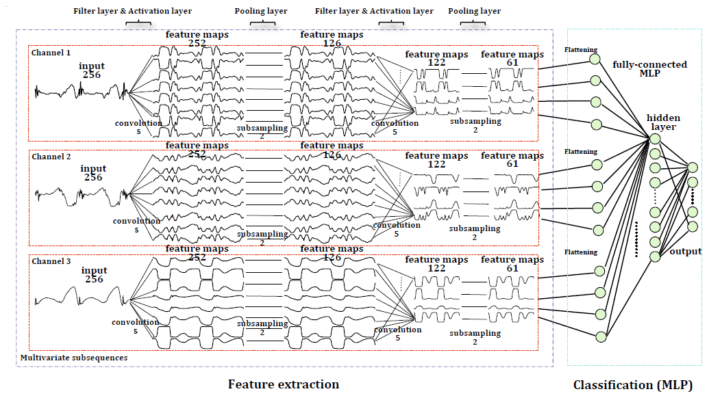
Figure 1 A two-stage MC-DCNN architecture for activity classification. This architecture consists of a three-channel input, two filter layers, two pooling layers, and two fully connected layers (after Zheng et al., 2014).

Brunel et al. (2019) present CNNs adapted for TSC in cosmology using 1-D filters to extract features from each channel over time and a convolution in depth to capture the correlation between the channels. They compared the results from LSTMs with those from CNNs and demonstrated that CNNs had better results. Nevertheless, both deep learning approaches are very promising.

The combination of CNNs and LSTM units has already yielded promising results in problems requiring temporal information classification, such as human activity recognition (Li et al., 2017; Mutegeki and Han, 2020), text classification (Luan and Lin, 2019; She and Zhang, 2018; Umer et al., 2020), video classification (Lu et al., 2018; and Wu et al., 2015), sentiment analysis (Ombabi et al., 2020; Sosa, 2017; Wang et al., 2016, 2019), typhoon formation forecasting (Chen et al., 2019), and arrhythmia diagnosis (Oh et al., 2018). In this architecture, convolutional operations capture features and LSTMs capture time dependencies on the extracted features. Ordóñez and Roggen (2016) propose a deep convolutional LSTM model (DeepConvLSTM) for activity recognition (Fig. 2). Their results are compared to the results from standard feedforward units showing that DeepConvLSTM reaches a higher F1 score and better decision boundaries for classification. Furthermore, they noticed that the LSTM model is also promising with relatively small datasets. Furthermore, LSTMs perform better with longer temporal dynamics, whereas the convolution filters can only capture the temporal dependencies dynamics within the length of the filter.

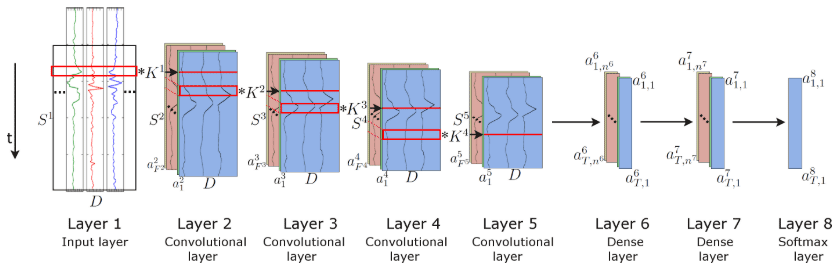
Figure 2 Architecture of the DeepConvLSTM framework used for activity recognition (after Ordóñez and Roggen, 2016).

The project presented in this paper is part of a greater project called DAVE, which aims at developing a tool for regional ice-jam watches and warnings, based on the integration of three aspects: current ice cover conditions, hydro-meteorological patterns associated with breakup ice jams, and channel predisposition to ice-jam formation. The outputs will be used to develop an ice-jam monitoring and warning module that will transfer the knowledge to the end users managing ice-jam consequences.

The objective of this research is to develop deep learning models to predict breakup ice-jam events to be used as an early warning system of possible flooding. While most TSC research in deep learning is performed on 1-D channels (Hatami et al., 2018), our approach consists of using deep learning frameworks for multivariate TSC, applied to ice-jam prediction. Through our comprehensive literature review, we noticed that CNN (e.g., Brunel et al., 2019; Cui et al., 2016; Devineau et al., 2018b; Kashiparekh et al., 2019; Nosratabadi et al., 2020; Yan et al., 2020; Yang et al., 2015; Yi et al., 2017; Zheng et al., 2016), LSTM (e.g., Fischer and Krauss, 2018; Lipton et al., 2015; Nosratabadi et al., 2020; Torres et al., 2021), and a combined CNN-LSTM (e.g., Karim et al., 2017; Livieris et al., 2020; Ordóñez and Roggen, 2016; Sainath et al., 2015; Xingjian et al., 2015) have been widely used for TSC. Numerous applications of CNN, LSTM, and their hybrid versions are currently used in the field of hydrology (Althoff et al., 2021; Apaydin et al., 2020; Barzegar et al., 2020, 2021; Kratzert et al., 2018; Wunsch et al., 2021; Zhang et al., 2018). Although deep learning methods seem promising to address the requirements of ice-jam predictions, none of these methods yet have been explored for ice-jam prediction.

Although machine learning methods have been widely used in time-series forecasting of hydro-meteorological data, they have been used less frequently in the prediction of ice jams (Graf et al., 2022). Semenova et al. (2020) used KNN to predict ice jams using hydro-meteorological variables such as precipitation, snow depth, water level, water discharge, and temperature. They developed their model with data collected from the confluence of the Sukhona River and Yug River in Russia between 1960 and 2016 and achieved accuracy of 82 %. Sarafanov et al. (2021) presented an ensemble-based model of machine learning methods and a physical snowmelt-runoff model to account for the advantages of physical models (interpretability) and machine learning models (low forecasting error). Their hybrid models proposed an automated approach for short-term flood forecasting in the Lena River, Poland, using hydro-meteorological variables (e.g., maximum water level, mean daily water and air temperature, mean daily water discharge, relative humidity, snow depth, and ice thickness). They applied an automated machine learning approach based on the evolutionary algorithm to automatically identify machine learning models, tune hyperparameters, and combine stand-alone models into ensembles. Their model was validated on 10 hydro-gauges for 2 years, showing that the hybrid model is much more efficient than stand-alone models with a Nash–Sutcliffe efficiency coefficient of 0.8. Graf et al. (2022) developed an MLP and extreme gradient boosting model to predict ice jams with data from 1983 to 2013, in the Warta River, Poland. They employed water and air temperatures, river flow, and water level as inputs to their models, showing that both machine learning methods provide promising results. In Canada, De Coste et al. (2021) developed a hybrid model including a number of machine learning models (e.g., KNN, SVM, random forest, and gradient boosting) for the St. John River (New Brunswick). The most successful ensemble model combining six different member models was produced with a prediction accuracy of 86 % over 11 years of record.

We developed three deep learning models – a CNN, an LSTM, and a combined CNN-LSTM for ice-jam predictions – and compared the results. The previous studies show that these models successfully capture features, the correlation between features (through convolution units), and time dependencies (through memory units), which are subsequently used for TSC. The combined CNN-LSTM can reduce errors by compensating for the internal weaknesses of each model. In the CNN-LSTM model, CNNs capture features, and then the LSTMs identify time dependencies on the captured features.

Furthermore, we also developed some machine learning methods as simpler methods for ice-jam prediction. And their results are compared with those obtained from the deep learning models.

2 Materials and methods

2.1 Data and study area

It is known that specific hydro-meteorological conditions lead to ice-jam occurrence (Turcotte and Morse, 2015; and White, 2003). For instance, breakup ice jams occur when a period of intense cold is followed by a rapid peak discharge resulting from spring rainfall and snowmelt runoff (Massie et al., 2002). Accumulated freezing degree days (AFDDs) can be used as a proxy for intense cold periods. Sudden spring runoff increase, however, is not often available at the jam location and can be represented by liquid precipitation and snow depth a few days prior to ice-jam occurrence (Zhao et al., 2012). Prowse and Bonsal (2004) and Prowse et al. (2007) assessed various hydroclimatic explanations for river ice freeze-up and breakup, concluding that shortwave radiation is the most critical factor influencing the mechanical strength of ice and consequently the possibility of breakup ice jams to occur. Turcotte and Morse (2015) explain that accumulated thawing degree day (ATDD), an indicator of warming periods, partially covers the effect of shortwave radiation. In previous studies addressing ice-jam and breakup predictions, discharge and changes in discharge, water level and changes in water level, AFDD, ATDD, precipitation, solar radiation, heat budget, and snowmelt or snowpack are the most frequently used variables (Madaeni et al., 2020).

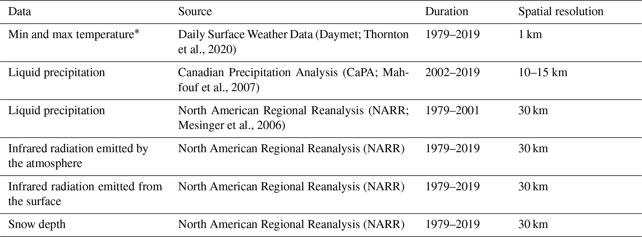
The inputs used in this study are historical ice-jam or no-ice-jam occurrence (Fig. 3) as well as hydro-meteorological variables from 150 rivers in Quebec, namely liquid precipitation (mm), minimum and maximum temperature (^∘C), AFDD (from 1 August ​​​​​​​ of each year; ^∘C), ATDD (from 1 January of each year; ^∘C), snow depth (cm), and net radiation (W m⁻²). The net solar radiation, which represents the total energy available to influence the climate, is calculated as the difference between incoming and outgoing energy. If the median temperature is greater than 1, precipitation is considered to be liquid. The statistics of hydro-meteorological data used in the models are presented in Table 1. The source, time period, and spatial resolution of the input variables are shown in Table 2.

Table 1 Statistics of hydro-meteorological variables used in the models.

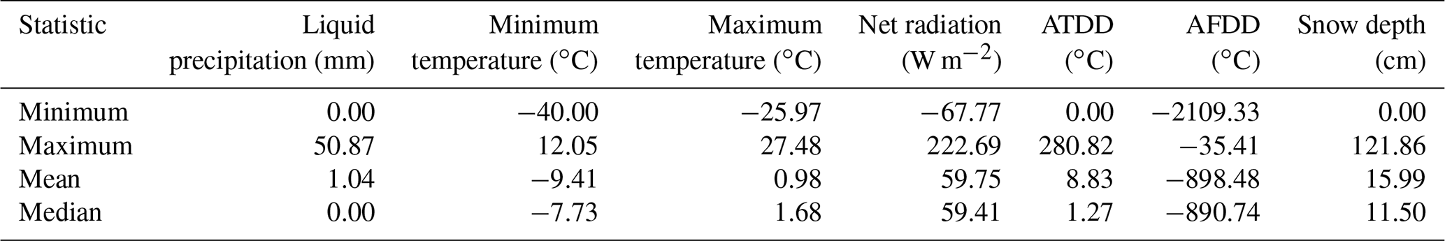
Table 2 Source, duration, and spatial resolution of hydro-meteorological data used in the models.

^* The average was used to derive the AFDD and the ATDD.

The ice-jam database was provided by the provincial public safety department (Ministère de la sécurité publique du Québec; MSPQ; Données Québec, 2021) for 150 rivers, mainly in the St. Lawrence River basin. The database comes from digital or paper events reported by local authorities under the jurisdiction of the MSPQ from 1985 to 2014. Moreover, other data used to build this database were provided by field observations collected by the Vigilance/Flood application from 2013 to 2019. It contains 995 recorded jam events that are not validated and contain many inaccuracies, mainly in the toponymy of the rivers, location, dating, and jam event redundancy.

The names of the watercourse of several recorded jams are not given, are wrong, or are misspelled. The toponymy of the rivers was corrected using the National Hydrographic Network (NHN; Government of Canada, 2021b), the GeoBase of the Quebec Hydrographic Network (Government of Canada, 2021a), and the Toporama Web Map Service (Government of Canada, 2020) of the Sector of Earth Sciences. Other manual corrections had to be carried out on ice-jam data. For example, ice jam location is sometimes placed on the riverbanks at a small distance (less than 20 m) from the river polygon. In this case, the location of the ice jam is manually moved inside the river polygon. In other cases, the ice-jam point is placed further on the flooded shore at a distance between 20 and 200 m from the true ice jam. This was corrected based on images with very high spatial resolution, based on the sinuosity and the narrowing of the river, the history of ice jams at the site, and press archives. In addition, some ice jams were placed too far from the river due to wrong coordinates in the database. A single-digit correction in longitude or latitude returned the jam to its exact location. There are certain cases where the date of jam formation is verified by searching press archives, notably when the date of formation is missing or several jams with the same dates and close locations in a section of a river are present.

The ice-jam database contains many duplicates. This redundancy can be explained by the merging of two databases, a double entry during ice-jam monitoring, or numerous recordings for an ice jam that lasted for several days. To remediate this, the duplicates were removed from the database. The corrected ice-jam database contains 850 jams for 150 rivers, mainly in southern Quebec (Fig. 3). Ice jams formed in November and December (freeze-up jams) are removed from the model since the processes involved are different from breakup ice jams (included from 15 January). The final breakup ice-jam database used in this study includes 504 jam events.

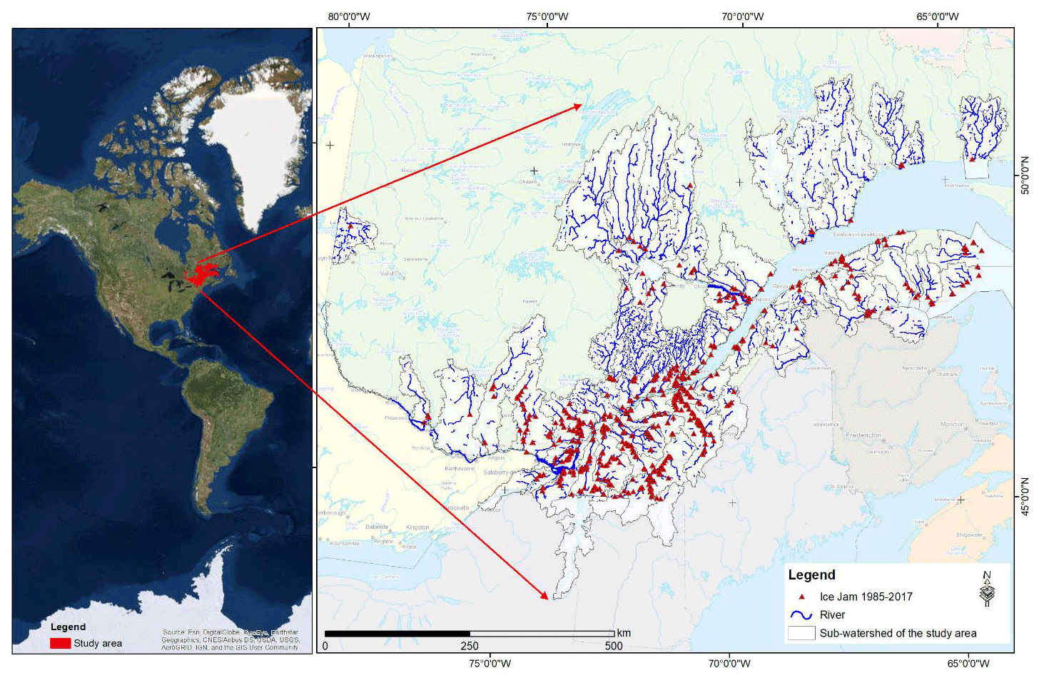
Figure 3 Study area and historic ice-jam locations recorded in Quebec from 1985 to 2017.

2.2 Machine learning models for TSC

The most common machine learning techniques used for TSC are SVM (Rodríguez and Alonso, 2004; Xing and Keogh, 2010), KNN (Li et al., 2013; Xing and Keogh, 2010), decision tree (DT; Brunello et al., 2019; Jović et al., 2012), and multilayer perceptron (MLP; del Campo et al., 2021; Nanopoulos et al., 2001). These models and their applications in TSC are beyond the scope of this study and will not be further addressed.

We developed the mentioned machine learning methods and compared their results with those of deep learning models. After some trials and errors, the parameters that are changed from the default values for each machine learning model are as follows. We developed an SVM with a polynomial kernel with a degree of 5 that can distinguish curved or nonlinear input space. The KNN is used with three neighbors used for classification. The decision tree model is applied with all the default values. The shallow MLP is used with the “lbfgs” solver (which can converge faster and perform better for small datasets), alpha of $\mathrm{1}\times {\mathrm{10}}^{-\mathrm{5}}$​​​​​​​, and three layers with seven neurons in each layer.

2.3 Deep learning models for TSC

The most common and popular deep neural networks for TSC are MLPs, CNNs, and LSTMs (Brownlee, 2018b; and Torres et al., 2021). Although it is a very powerful approach, MLP networks are limited by the fact that each input (i.e., time-series element) and output are treated independently, which means that the temporal or space information is lost (Lipton et al., 2015). Hence, an MLP needs some temporal information in the input data to model sequential data, such as time series (Ordóñez and Roggen, 2016). In this regard, recurrent neural networks (RNNs) are specifically adapted to sequence data through the direct connections between individual layers (Jozefowicz et al., 2015). Recurrent neural networks perform the same repeating function with a straightforward structure, e.g., a single tanh (hyperbolic tangent) layer, for every input of data (xt), and the inputs are related to each other within their hidden internal state, which allows it to learn the temporal dynamics of sequential data (Fig. 4).

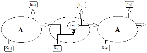
Figure 4 An RNN with a single tanh layer, where A is a chunk of the neural network, x is input data, and h is output data.

Recurrent neural networks are rarely used in TSC due to their significant limitations: RNNs mostly predict outputs for each time-series element; they are sensitive to the first examples seen, and it is challenging to capture long-term dependencies due to vanishing gradients, exploding gradients, and their complex dynamics (Devineau et al., 2018b; Fawaz et al., 2019b).

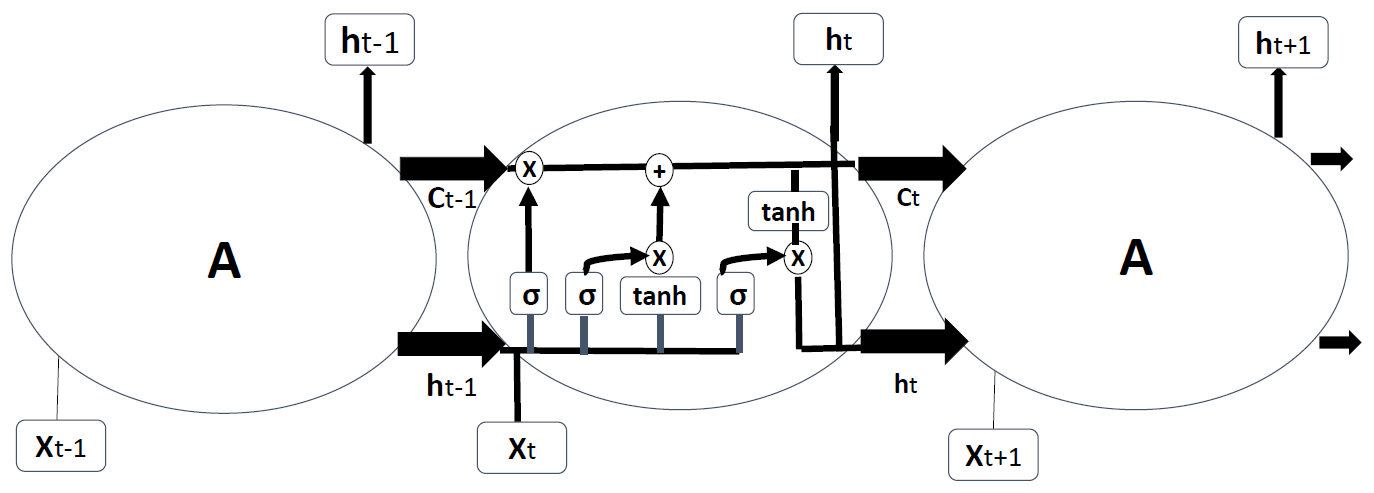
Long short-term memory RNNs are developed to improve the performance of RNNs by integrating a memory component to model long-term dependencies in time-series problems (Brunel et al., 2019; Karim et al., 2019a). Long short-term memory networks do not have the problem of exploding gradients. The LSTMs have four interacting neural network layers in a very special way (Fig. 5). An LSTM has three sigmoid (σ) layers to control how much of each component should be let through by outputting numbers between zero and one. The input to an LSTM goes through three gates (“forget”, “input”, and “output” gates) that control the operation performed on each LSTM block (Ordóñez and Roggen, 2016). The first step is the “forget gate” layer that gets the output of the previous block (​​​​​​​h_t−1), the input for the current block (X_t), and the memory of the previous block (C_t−1) and gives a number between 0 and 1 for each number in the cell state (C_t−1; Understanding LSTM Networks, 2021). The second step is called the “input gate” with two parts, a sigmoid layer that decides which values to be updated and a tanh layer that creates new candidate values for the cell state. The new and old memories are then be combined and control how much the new memory should influence the old memory. The last step (output gate) gives the output by applying a sigmoid layer deciding how much new cell memory goes to output and multiplies it by tanh applied to the cell state (resulting in values between −1 and 1).

Figure 5 Structure of LSTM block with four interacting layers.

Recently, convolutional neural networks challenged the assumption that RNNs (e.g., LSTMs) have the best performance when working with sequences. Convolutional NNs perform well when processing sequential data such as speech recognition and sentence classification, similar to TSC (Fawaz et al., 2019b).

Convolutional NNs are the most widely used deep learning methods in TSC problems (Fawaz et al., 2019b). They learn spatial features from raw input time series using filters (Fawaz et al., 2019b). Convolutional NNs are robust and need a relatively small amount of training time compared to RNNs or MLPs. They work best for extracting local information and reducing the complexity of the model.

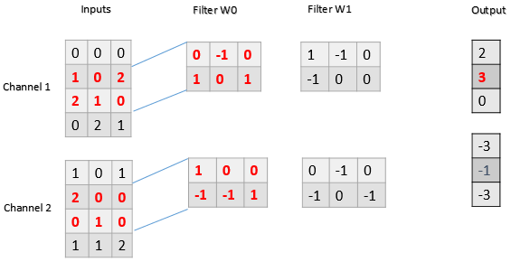
A CNN is a kind of neural network with at least one convolutional (or filter) layer. A CNN usually involves several convolutional layers, activation functions, and pooling layers for feature extraction, followed by dense layers used as classifiers (Devineau et al., 2018b). The reason to use a sequence of filters is to learn various features from time series for TSC. A convolutional layer consists of a set of learnable filters that compute dot products between local regions in the input and corresponding weights. With high-dimensional inputs, it is impractical to connect subsequent neurons to all the neurons of the previous layer. Therefore, each neuron in CNNs is connected to only a local region of the input – receptive field – whose size is equivalent to that of the filter (Fig. 6). This feature reduces the number of parameters by limiting the number of connections between neurons in different layers. The input is first convolved with a learned filter, and then an element-wise nonlinear activation function is applied to the convolved results (Gu et al., 2018). The pooling layer performs a downsampling operation such as maximum or average, reducing the spatial dimension. One of the most powerful features of CNNs is called weight or parameter sharing, where all neurons share filters (weights) in a particular feature map (Fawaz et al., 2019b). This allows us to reduce the number of parameters.

Figure 6 Structure of a convolution layer including two sets of filters.

2.4 Model libraries

In an Anaconda (Anaconda Software Distribution, 2016) environment, Python is implemented to develop CNN, LSTM, and CNN-LSTM networks for TSC. To build and train networks, the networks are implemented in Theano (Bergstra et al., 2010) using the Lasagne library (Dieleman et al., 2015). Other core libraries used for importing, preprocessing, training data, and visualization of results include Pandas (Reback et al., 2020), NumPy (Harris et al., 2020), scikit-learn (Pedregosa et al., 2011), and Matplotlib. PyLab (Hunter, 2007). The Spyder (Spyder-Documentation, 2009) package of Anaconda can be used as an interface; otherwise, the command window can be used without any interface.

To develop machine learning models, scikit-learn machine learning libraries are used except for NumPy, Pandas, and scikit-learn preprocessing libraries.

2.5 Preprocessing

The data are comprised of variables with varying scales, and the machine-learning algorithms can benefit from rescaling the variables to all have one single scale. Scikit-learn (Pedregosa et al., 2011) is a free library for machine learning in Python that can be used to preprocess data. We examined scikit-learn MinMaxScaler (scaling each variable between 0 and 1), Normalizer (scaling individual samples to the unit norm), and StandardScaler (transforming to zero mean and unit variance separately for each feature). The results show that MinMaxScaler (Eq. 1) leads to the most accurate results. Validation data rescaling is carried out based on minimum and maximum values of the train data.

$$\begin{array}{}\text{(1)}& X_{\mathrm{scaled}}={\displaystyle \frac{X-X_{min}}{X_{max}-X_{min}}}\end{array}$$

For ​​​​​​​ each jam or no-jam event, the data from 15 d preceding the event were used to predict the event on the 16th day. A balanced dataset with the same number of jam and no-jam events (1008 small sequences) was generated, preventing the model from becoming biased to jam or no-jam events. The hydro-meteorological data related to no-jam events were constructed by extracting data from the reaches of no-jam records. Model generalizations were assessed by extracting 10 % of data for testing. With the remaining data, 80 % was used for training and 20 % for validation. We used the ShuffleSplit subroutine from the scikit-learn library, where the database was randomly sampled during each reshuffling and splitting iteration to generate training and validation sets. We applied 100 reshuffling and splitting iterations for training and validation. There are 726, 181, and 101 small sequences for training, validation, and testing, respectively, with the size of (16, 7), 16 d of data for the seven variables.

2.6 Training

Training a deep neural network with an excellent generalization to new unseen inputs is challenging. As a benchmark, a CNN model with parameters and layers similar to previous studies (e.g., Ordóñez and Roggen, 2016) is developed. The model shows underfitting or overfitting with various architectures and parameters. To overcome underfitting, deeper models and more nodes can be added to each layer; however, overfitting is more challenging to resolve. The ice-jam dataset for Quebec contains 1008 balanced sequence instances (with a length of 16), which is considered to be a small amount of data in the context of deep learning. Deep learning models tend to overfit small datasets by memorizing inputs rather than training. This is due to the fact that small datasets may not appropriately describe the relationship between input and output spaces.

2.6.1 Overcome overfitting

There are various ways to resolve the problem of overfitting, including acquiring more data, data augmentation (e.g., cropping, rotating, and noise injection), dropout (Srivastava et al., 2014), early stopping, batch normalization (Ioffe and Szegedy, 2015), and regularization. Acquiring more data is not possible with ice-jam records. We added the Gaussian noise layer (from the Lasagne library), where the noise values are Gaussian-distributed with zero mean and a standard deviation of 0.1 to the input. The noise layers applied to the CNN and LSTM models significantly overcome the overfitting problem through data augmentation. However, the performance of the CNN-LSTM model dramatically deteriorates when a noise layer is added (Fig. 7). Adding a noise layer to other layers does not improve any of the developed models for ice-jam prediction.

Figure 7 Train and validation errors over epochs for CNN-LSTM model with a noise layer.

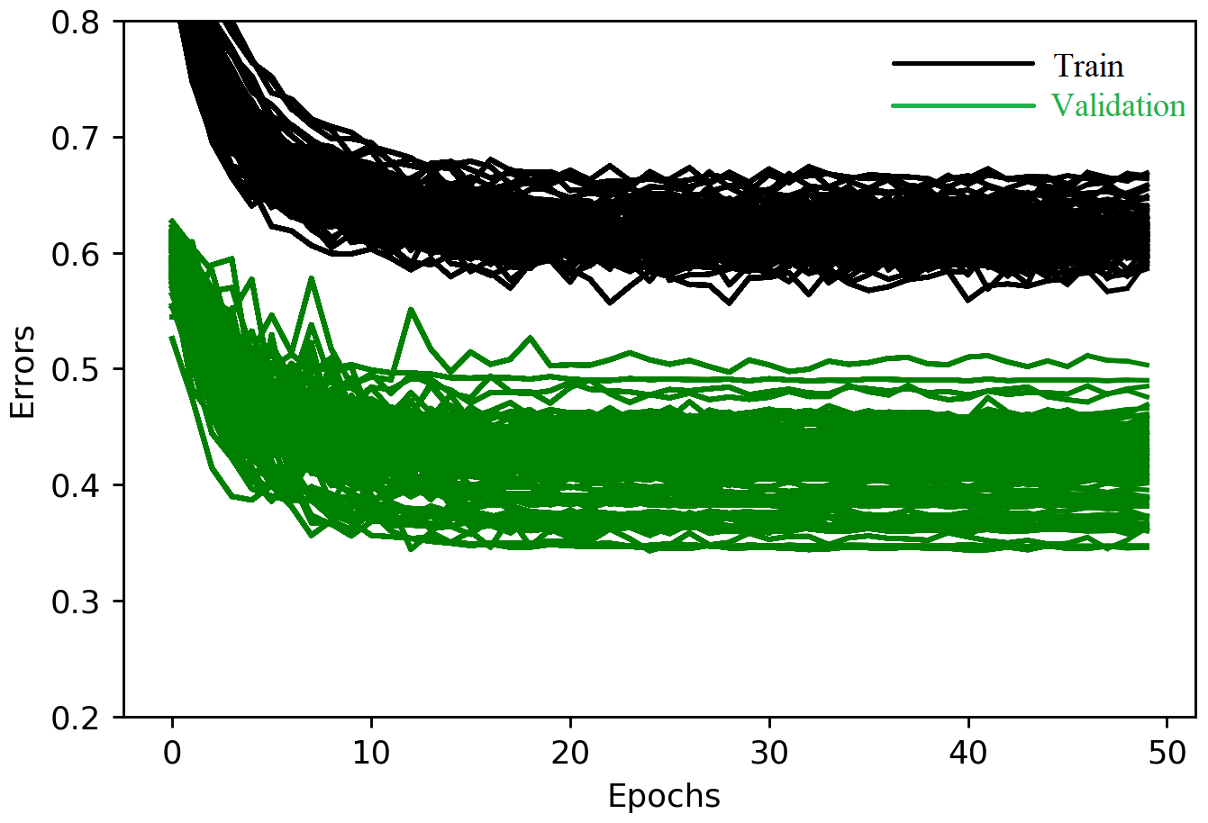
Early stopping is another efficient method that halts the training procedure at a point where further training would decrease training loss, but validation loss starts to increase. Neural networks need a loss function to guide optimization problem resolution. The loss function is similar to an objective function for process-based hydrological models. Among the developed models, only LSTM needs early stopping at 40 epochs (Fig. 8). More detailed explanations about the methods that are used in this study to overcome overfitting (e.g., batch normalization and L2 regularization) can be found in the Appendix.

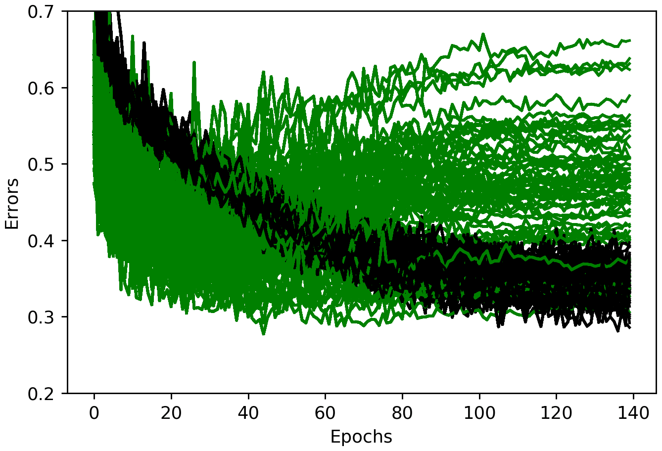
Figure 8 Train and validation errors over epochs for an LSTM model showing overfitting after 40 epochs.

2.6.2 Model hyperparameters

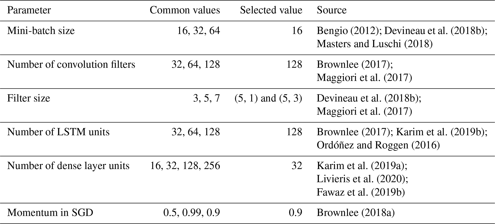
Finding hyperparameter values has been challenging due to the complex architecture of deep learning models and the large number of parameters (Garbin et al., 2020). The best model architecture was identified by assessing model performance with different layers and parameters such as the number of layers (noise, batch normalization, convolutional, pooling, LSTM, dropout, and dense) as well as different pooling sizes and strides, different batch sizes, various scaling of data (standardization and normalization), various filter sizes, number of units in LSTM and dense layers, the type of the activation functions, regularization and learning rates, weight decay, and number of filters in convolutional layers. Hyperparameters are optimized through manual trial and error searches as grid search experiments suffer from poor dimensional coverage in dimensions (Bergstra and Bengio, 2012). Another reason is that manual experiments are much easier to conduct and interpret when investigating the effect of one hyperparameter of interest. The optimized hyperparameters are presented in Table 3. The most important parameters of the models are explained below, and additional information is available in the Appendix.

Table 3 Common and selected values for different parameters of the models.

Number of layers

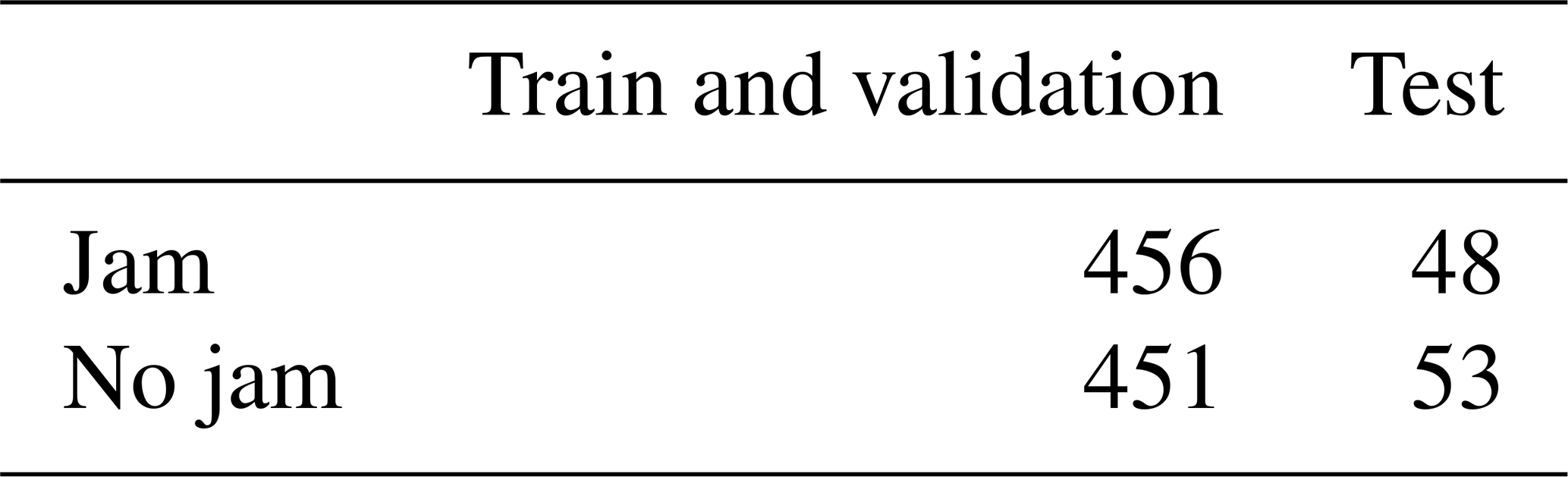
The depth of models is related to the sequence length (Devineau et al., 2018a), as deeper networks need more data to provide better generalization (Fawaz et al., 2019a). In previous studies focused on CNNs, there were usually one, two, or three convolution stages (Zheng et al., 2014). We tried different numbers of CNN, LSTM, and dense layers, and the best combination was obtained with three CNN layers, two LSTM layers, and two dense layers. The sequence length in this study is small (16), and model performance was not improved by simply increasing depth.

Number and size of convolution filters

Data with more classes need more filters, and longer time series need longer filters to capture longer patterns and consequently to produce accurate results (Fawaz et al., 2019a). However, longer filters significantly increase the number of parameters and potential for overfitting small datasets, while a small filter size risks poor performance. In this study, two convolutional layers with 1-D filters of size (5, 1) and stride of (1, 1) were used to capture temporal variation for each variable separately. Furthermore, one convolutional layer with 2-D filters of size (5, 3) and stride of (1, 1) was used to capture the correlation between variables via depth-wise convolution of input time series. A big stride might cause the model to miss valuable data used in predicting and smoothing out the noise in the time series. The layers in CNNs have a bias for each channel, sharing across all positions in each channel.

Adaptive learning rates

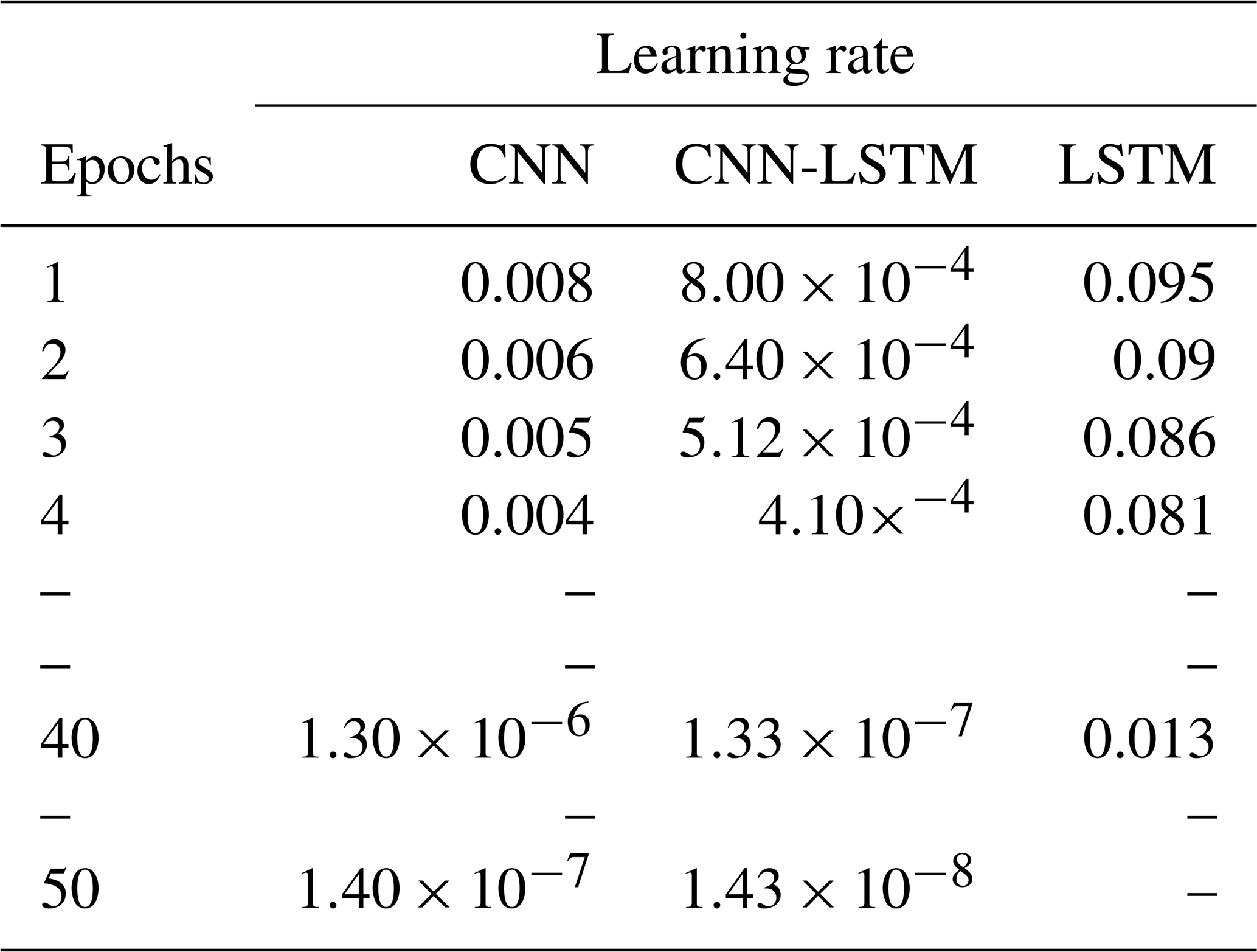
The adaptive learning rate decreases the learning rate and consequently weights over each epoch. We tried different base learning and decay rates for each model and found that the learning rate significantly impacts the model's performance. Finally, we chose a base learning rate of 0.1, 0.01, and 0.001 for LSTM, CNN, and CNN-LSTM, respectively. A decay rate of 0.8 was used for CNN and CNN-LSTM and a rate of 0.95 for the LSTM model. Table 4 shows the adaptive learning rates for CNN, LSTM, and CNN-LSTM calculated using Eq. (2) for each epoch.

$$\begin{array}{}\text{(2)}& \text{adaptive learning rate}=\text{base learning rate}\times {\mathrm{decay}}^{\mathrm{epoch}}\end{array}$$

The experiments show that the learning rate is the most critical parameter influencing the model performance. A small learning rate can cause the loss function to get stuck in local minima, and a large learning rate can result in oscillations around global minima without reaching it.

Our CNN-LSTM model is deeper than the other two models, and deeper models are more prone to a vanishing gradient problem. To overcome the vanishing gradients, it is generally recommended to use lower learning rates, e.g., lower than $\mathrm{1}\times {\mathrm{10}}^{-\mathrm{4}}$​​​​​​​. Interestingly, we found that our CNN-LSTM model works better with lower learning rates than the other two models.

Table 4 The adaptive learning rate for 50 epochs.

2.6.3 Model evaluation

The network on the validation set is evaluated after each epoch during training to monitor the training progress. During validation, all non-deterministic layers are switched to deterministic. For instance, noise layers are disabled, and the update step of the parameters is not performed.

The classification accuracy cannot appropriately represent model performance for unbalanced datasets, as the model can show a high accuracy by biasing towards the majority class in the dataset (Ordóñez and Roggen, 2016). While we built a balanced dataset (with the same number of jam and no-jam events), randomly selecting test data, shuffling the inputs, and splitting data into train and validation sets can result in a slightly unbalanced dataset. In our case, the number of jams and no jams for train and validation and test sets is presented in Table 5. Therefore, the F1 score (Eq. 3), which considers each class equally important, is used to measure the accuracy of binary classification. The F1 score, as a weighted average of the precision (Eq. 4) and recall (Eq. 5), ranges between 0 and 1, where 0 is the worse score and 1 is the best. In Eqs. (4) and (5), TP, FP, and FN are true positive, false positive, and false negative, respectively.

$$\begin{array}{}\text{(3)}& {\displaystyle }\mathrm{F}\mathrm{1}=\mathrm{2}\times {\displaystyle \frac{\mathrm{precision}\times \mathrm{recall}}{\mathrm{precision}+\mathrm{recall}}}\text{(4)}& {\displaystyle }\mathrm{Precision}={\displaystyle \frac{\mathrm{TP}}{\mathrm{TP}+\mathrm{FP}}}\text{(5)}& {\displaystyle }\mathrm{Recall}={\displaystyle \frac{\mathrm{TP}}{\mathrm{TP}+\mathrm{FN}}}\end{array}$$

Although the model accuracy is usually used to examine the performance of deep learning models, the model size (i.e., number of parameters) provides a second metric, which represents required memory and calculations, to be compared among models with the same accuracy (Garbin et al., 2020).

Table 5 The number of jam and no-jam events used in the rain and validation and test datasets.

After training the model, the well-trained network parameters are saved to a file and are later used to test network generalizations using the test dataset, composed of data that are not used during training and validation.

2.7 Architecture of models

The final architecture of CNN, LSTM, and CNN-LSTM models is presented in Figs. 9, 10, and 11, respectively. The layers, their output shapes, and their number of parameters are respectively presented in Tables 6, 7, and 8 for CNN, LSTM, and CNN-LSTM models.

Convolutional NN models often include pooling layers to reduce data complexity and dimensionality. However, it is not always necessary for every convolutional layer to be followed by a pooling layer in the time-series domain (Ordóñez and Roggen, 2016). For instance, Fawaz et al. (2019a) do not apply any pooling layers in their TSC models. We tried max-pooling layers after different convolutional layers in CNN and CNN-LSTM networks and found that a pooling layer following only the last convolutional layer improves the performance of both models. This can be due to subsampling the time series and using time series with a length of 16 that eliminates the need for decreased dimensionality.

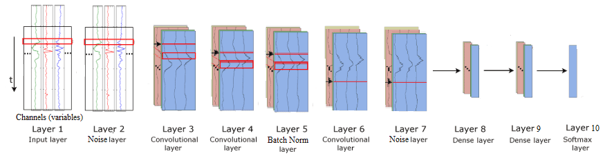
Figure 9 Architecture of the CNN model for ice-jam prediction (adapted after Ordóñez and Roggen, 2016).

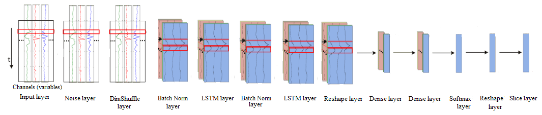
Figure 10 Architecture of the LSTM model for ice-jam prediction (adapted after Ordóñez and Roggen, 2016).

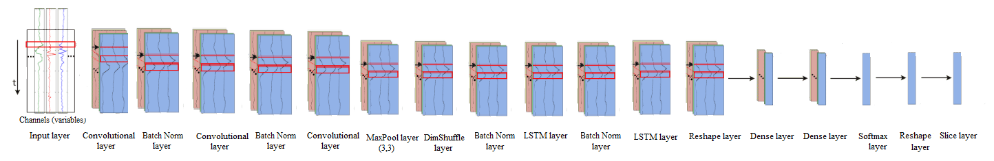
Figure 11 Architecture of the CNN-LSTM model for ice-jam prediction (adapted after Ordóñez and Roggen, 2016).

Table 6 Layers, output shapes, and number of parameters for the CNN model.

Table 7 Layers, output shapes, and number of parameters for the LSTM model.

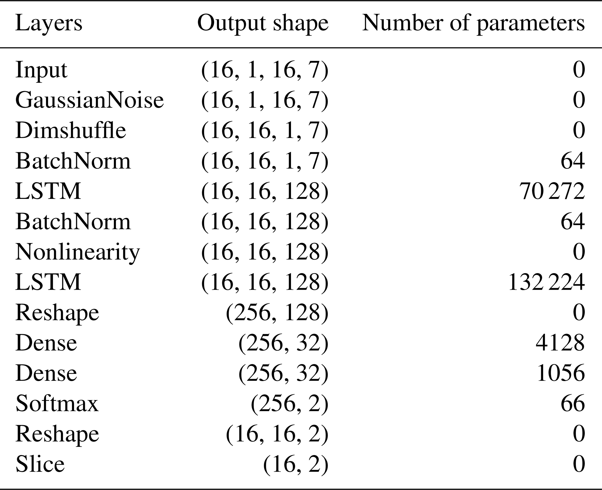
Table 8 Layers, output shapes, and number of parameters for the CNN-LSTM model.

3 Results and discussion

3.1 Weight initialization

Among all the methods available for weight initialization in the Lasagne library, Glorot uniform (i.e., Glorot and Bengio, 2010) and He initializations (He et al., 2015) are the most popular initialization techniques to set the initial random weights in convolutional layers. The results reveal that in our case, these methods yield comparable F1 scores. However, the histograms of F1 scores reveal that Glorot uniform yields slightly better results (Fig. 12).

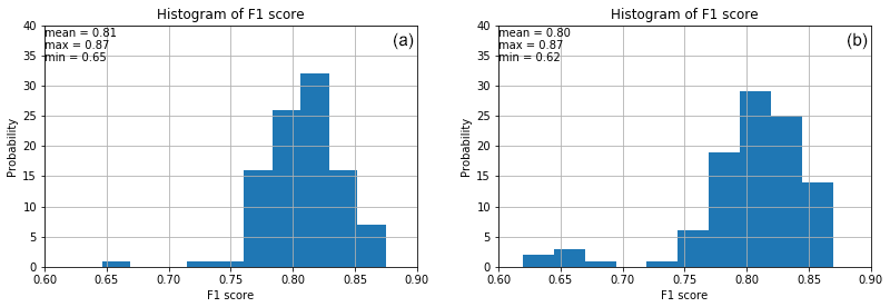
Figure 12 Histograms of F1 score for CNN using He (a) and Glorot uniform (b) weight initialization with 100 random training–validation splits.

3.2 Model evaluation

3.2.1 Learning curves and F1 scores

Line plots of the loss (i.e., learning curves), which are the loss over each epoch, are widely used to assess model performance in machine learning. Furthermore, line plots clearly indicate common learning problems, such as underfitting and overfitting. The learning curves for CNN, LSTM, and CNN-LSTM models are presented in Fig. 13. The LSTM model starts to overfit at epoch 40, so an early stopping is conducted. CNN-LSTM performs better than the other two models, as its training loss is the lowest and is lower than its validation loss. Histograms of F1 scores (Fig. 14 and Table 9) show that CNN-LSTM outperforms the other two models since it results in the highest average and the highest minimum F1 scores for validation (0.82 and 0.75, respectively). Figure 13 shows that the training error of the CNN model is lower than that of the LSTM model, indicating that it trained more efficiently. However, it is not true for the validation error. The validation error is less than the training error in the LSTM model because of the regularization methods used, as LSTM models are often harder to regularize, agreeing with previous studies (e.g., Devineau et al., 2018b).

The LSTM network is validated better than the CNN model since its average and minimum F1 scores for validation are better than the CNN model (by 1 % and 32 %, respectively), and also LSTM yielded no F1 scores below 0.74 (Fig. 14 and Table 9).

As shown in Fig. 13, training loss is higher than validation loss in some of the results. There are some reasons explaining that. Regularization reduces the validation loss at the expense of increasing training loss. Regularization techniques such as the application of noise layers are only used during training but not during validation, resulting in smoother and usually better functions in validation. There is no noise layer in CNN-LSTM model that could result in a lower training error than the validation error. However, other regularization methods such as L2 regularization are used in all the models, including the CNN-LSTM model.

Furthermore, batch normalization uses the mean and variance of each batch during the training phase, whereas it uses the mean and variance of the whole training dataset in the validation phase. Additionally, training loss is averaged over each epoch, while validation losses are calculated upon completion of each training epoch. Hence, the training loss includes error calculations with fewer updates.

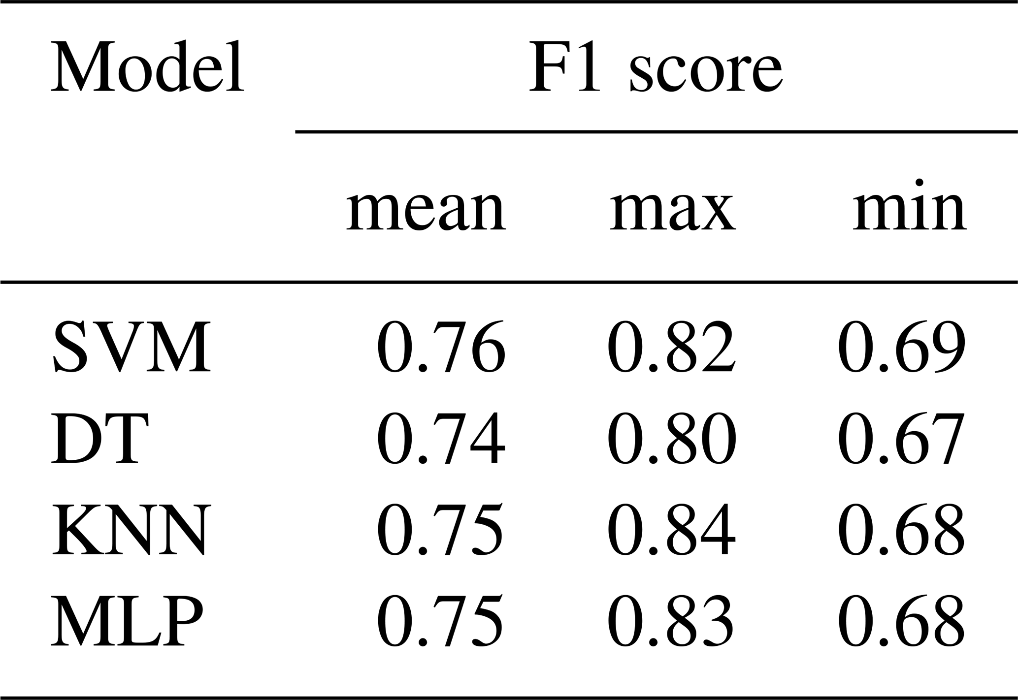
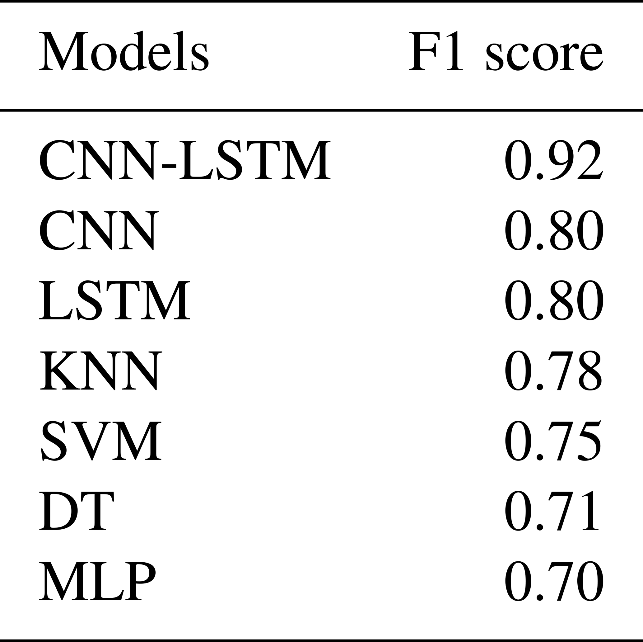
Among the developed machine learning models, SVM shows the best validation performance (Fig. 15 and Table 10). However, F1 scores of deep learning models are much higher than those of machine learning models with an average of 6 % higher F1 score resulting from the CNN-LSTM model compared to the SVM model (Tables 9 and 10).

Table 9 F1 scores of the validation phase for CNN, LSTM, and CNN-LSTM models with 100 random training–validation splits.

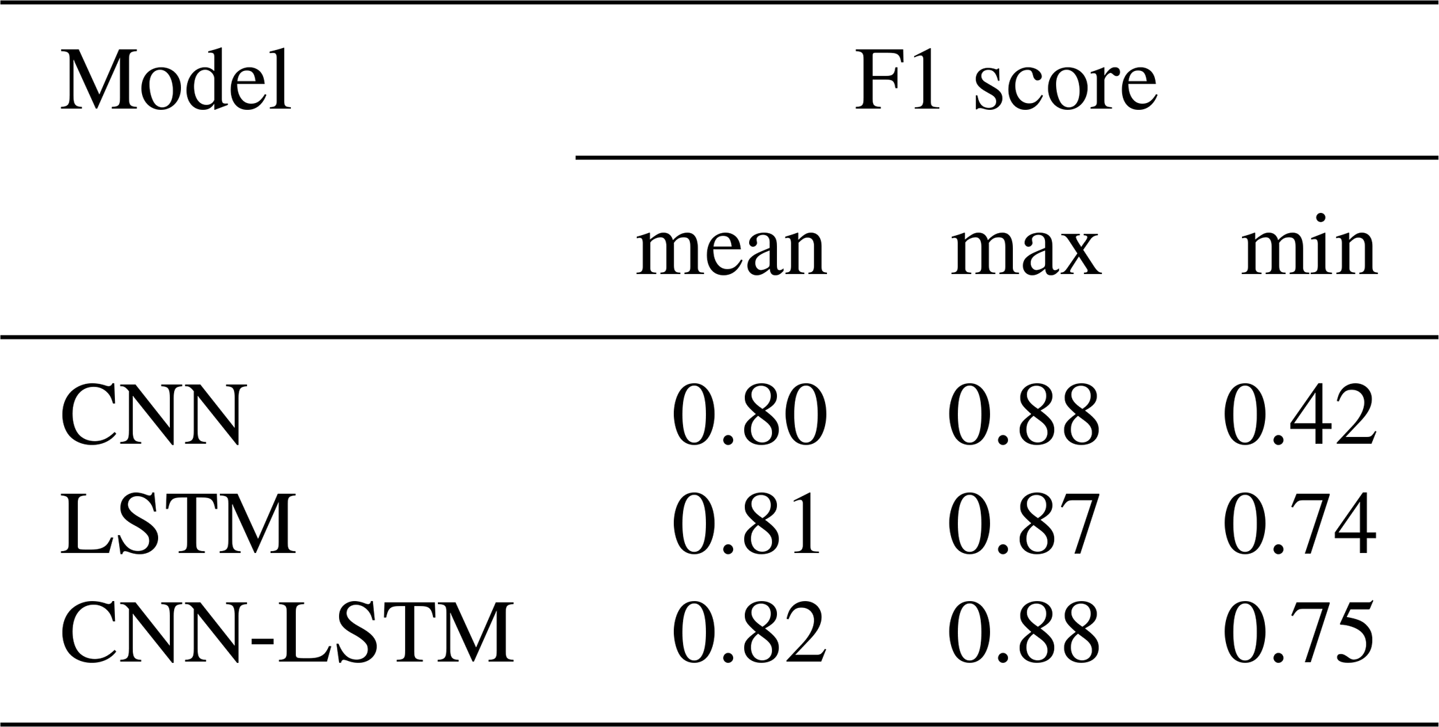
Table 10 F1 scores of the validation phase for SVM, DT, and KNN and MLP models with 100 random training–validation splits.

3.2.2 Number of parameters and run time

The total number of parameters in CNN, LSTM, and CNN-LSTM networks are 371 586, 207 874, and 664 746, respectively. The CNN-LSTM model had the best performance with the highest number of parameters. Even though the number of parameters for the LSTM model is less than that of the CNN model, the LSTM model shows better validation performance. Furthermore, the number of parameters in the CNN-LSTM model is much higher than the other two models, without a large increase in computation time. All three models were trained within 24 h using 100 shuffle splits for training and validation. The models were run on a CPU with four cores, 3.4 GHz clock speed, and 12 GB RAM. On the other hand, a few minutes were enough to train the machine learning models with 100 shuffle splits for training and validation. Although the training time for deep learning models is much higher than that of machine learning models, their superior performance, in this case, justifies their application.

3.3 Order of input variables

It is not clear whether the order of input variables in the input file influences multivariate TSC or not when using 2-D filters and 2-D max-pooling layers. In the benchmark model, the variables were entered from left to right in the following random order: precipitation, minimum temperature, maximum temperature, net radiation, ATDD, AFDD, and snow depth. Another run was conducted by changing the order of the variables for the following random order: snow depth, maximum temperature, precipitation, AFDD, net radiation, minimum temperature, and ATDD. Both models yielded the same mean and minimum F1 scores, whereas the maximum F1 score of the benchmark model is higher (0.88) than that of the comparative run (0.86). Therefore, it can be concluded that the order does not significantly impact the results.

3.4 Testing

To examine the ability of the models to generalize to new unseen data, we randomly set aside 10 % of the data from the training and validation phase of all the developed deep learning and machine learning models. A CNN, an LSTM, and a CNN-LSTM model were trained, and the well-trained parameters were saved and used to assess the model's ability to generalize. An SVM, a DT, a KNN, and an MLP model were also trained. The trained models were saved and used for testing. The test dataset is nearly balanced with 101 samples with the size of (16, 7), including 48 jam events and 53 no-jam events.

The results of the test models show that the CNN-LSTM model had the best F1 score of 0.92 (Table 11). Tables 9 and 11 show that although LSTM had a slightly superior validation performance, CNN and LSTM models performed the same in testing.

Testing results of machine learning models are presented in Table 11. Among the machine learning models, KNN yields the best results with F1 scores of 78 %. By comparing the best deep learning model (CNN-LSTM) with the best machine learning model (KNN), it can be calculated that the deep learning model outperforms the machine learning model by a difference of 14 % (F1 score of 92 % and 78 %, respectively).

Table 11 Test F1 scores for the developed deep learning and machine learning models.

3.5 Model comparison

Classifiers can be combined and used in pattern recognition problems to reduce errors by covering for one another's internal weaknesses (Parvin et al., 2011). Combined classifiers may be less accurate than the most accurate classifier; however, the accuracy of the combined model is always superior to the average accuracy of individual models. Combining two models improved our results compared to convolution-only or LSTM-only networks in both training and testing, supporting the previous studies (e.g., Sainath et al., 2015). It can be because the CNN-LSTM model incorporates both the temporal dependency of each variable by using LSTM networks and the correlation between variables through CNN models. The combined CNN-LSTM model efficiently benefits from automatic feature learning by CNN plus the native support for time series by LSTM.

Although LSTM slightly outperformed CNN in the validation phase, these models had comparable performance in the testing phase. The CNN is able to partially include both temporal dependency and the correlation between variables by using 1-D and 2-D filters, respectively. Although the LSTM is unable to incorporate the correlations between variables, it gives promising results with a relatively small dataset. Another difference is that LSTM captures longer temporal dynamics, while the CNN only captures temporal dynamics comprised within the length of its filters.

Even though our training data in supervised ice-jam prediction are small, the results reveal that deep learning techniques can give accurate results, which agrees with a previous study conducted by Ordóñez and Roggen (2016) in activity recognition. The excellent performance of CNN and CNN-LSTM models may be partially due to the characteristic of CNN that decreases the total number of parameters which does training with limited training data easier (Gao et al., 2016). However, we expect our models to be improved in the future by a larger dataset.

Among the developed machine learning models, SVM showed the best performance in validation, whereas KNN worked the best in testing. However, the performance of deep learning models is much better than machine learning models in both validation and testing. The machine learning models do not consider correlations between variables. However, it is not the only reason that deep learning models worked better than machine learning models, as the LSTM also does not consider correlations between variables but worked better than machine learning models. This indicates that there are other aspects of deep learning models that contribute to their high performance level. For instance, deep learning models perform well for the problems with complex nonlinear dependencies, time dependencies, and multivariate inputs.

The developed CNN-LSTM model can be used for future predictions of ice jams in Quebec to provide early warning of possible floods in the area by using historic hydro-meteorological variables and their predictions for some days in advance.

3.6 Discussion on the interpretability of deep learning models

Even though the developed deep learning models performed well in predicting ice jams in Quebec, the interpretability of the results with respect to the physical processes involved in ice jams is still essential. It is because although deep learning models have achieved superior performance in various tasks, these complicated models use a large number of parameters and might sometimes exhibit unexpected behaviors (Samek et al., 2017; Zhang et al., 2021). This is because the real-world environment is still much more complex than any model. Furthermore, the models may learn some spurious correlations in the data and make correct predictions for the wrong reason (Samek and Müller, 2019). Hence, interpretability is especially important in some real-world applications like flood and ice-jam predictions where an error could have catastrophic consequences. Nonetheless, interpretability can be used to extract novel domain knowledge and hidden laws of nature in the research fields with limited domain knowledge (Alipanahi et al., 2015) like ice-jam prediction.

However, the nested nonlinear structure and the “black box” nature of deep neural networks make the interpretation of their underlying mechanisms and decisions a significant challenge (Montavon et al., 2018; Zhang et al., 2021; Wojtas and Chen, 2020). That is why deep neural network interpretability still remains a young and emerging field of research. Nevertheless, there are various methods available to facilitate the understanding of decisions made by a deep learning model such as feature importance ranking, sensitivity analysis, layer-wise relevance propagation, and the global surrogate model. However, the interpretability of developed deep learning models for ice-jam prediction is beyond the scope of this study, and it will be investigated in our future works.

3.7 Model transferability

The transferability of a model between river basins is highly desirable but has not yet been achieved because most river ice-jam models are site-specific (Mahabir et al., 2007). The developed models in this study can be used to predict future ice jams some days before the event not only for Quebec but can also be transferred to eastern parts of Ontario and western New Brunswick, since these areas have the similar hydro-meteorological conditions. For other locations, the developed models could be retrained with a small amount of fine-tuning using labeled instances rather than building from scratch. This interesting feature is due to the logic behind the model, which could be transferred to other sites with small modifications. To transfer a model from one river basin to another, historical records of ice jams and equivalent hydro-meteorological variables (e.g., precipitation, temperature, and snow depth) must be available as model inputs for each site.

4 Conclusion

The main finding from this project is that the developed deep models successfully predicted ice jams in Quebec and performed much better than the developed machine learning models. The results show that the CNN-LSTM model is superior to the CNN-only and LSTM-only networks in both validation and testing phases, although the LSTM and CNN performed well.

To our best knowledge, this study is the first to apply deep learning models to the ice-jam prediction. The developed models are promising tools for the prediction of ice jams in Quebec and other similar river basins in Canada, with retraining and a small amount of fine-tuning.

The developed models do not apply to freeze-up jams that occur in early winter and are based on different processes than breakup jams. We studied only breakup ice jams as usually they result in flooding and are more dangerous than freeze-up jams. Furthermore, there is a lack of data availability for freeze-up ice jams in Quebec, and only 89 records of freeze-up jams are available, which is too small.

The main limitation of this study is the availability of ice-jam records. Indeed, small datasets may lead deep learning models to overfit the data. Another limitation of the presented work is the lack of interpretability of the results with respect to the physical characteristics of the ice jam. This is a topic of future research and our next step is to explore that.

It should also be noted that hydro-meteorological variables are not the only drivers of ice-jam formation. Geomorphological features such as river slope, sinuosity, physical barriers (such as an island or a bridge), channel narrowing, and river confluence also govern the formation of ice jams. In the future, a geospatial model using deep learning will be developed to examine the impacts of these geospatial parameters on ice-jam formation.

Appendix A: Overcome overfitting

A1 Noise layer

Although data augmentation is common in image classification (Wong et al., 2016), the application of data augmentation in deep learning for time-series classification (TSC) still has not been studied thoroughly (Fawaz et al., 2019b). A simple form of random data augmentation that can be used for TSC is a noise layer. Over the training process, each time an input sample is exposed to the model, the noise layer creates new samples in the vicinity of the training samples, resulting in various input data every time. The noise layer is usually added to the input data but can also be added to other layers.

A2 Dropout

The dropout (Srivastava et al., 2014) is the most successful method for neural network regularization that randomly sets some nodes in different layers to zero (Fig. A1). We used dropout with the recommended rates of 0.1 for the input layer and between 0.5 and 0.8 for hidden layers (Garbin et al., 2020) in our models, but it could not improve any developed models. This agrees with previous studies revealing that dropout does not work well with long short-term memories (LSTMs) (Zaremba et al., 2014) and convolutional neural networks (CNNs), and dropout layers do not work when batch size is small (less than 256; Garbin et al., 2020). Furthermore, it is in agreement with Garbin et al. (2020) stating that utilizing batch normalization layers in a model reduces the need for dropout layers.

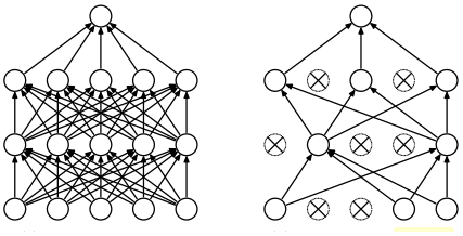
Figure A1 A neural network with two hidden layers (left) and a neural network with dropout (right; after Srivastava et al., 2014).

A3 Batch normalization

As explained earlier, the input data are scaled separately for each feature to be between 0 and 1. However, in deep learning, the distribution of the input of each layer will be changed by updates to all the preceding layers (i.e., internal covariate shift). Hence, hidden layers try to learn to adapt to the new distribution slowing down the training process. To solve these problems, a recent method called batch normalization (Ioffe and Szegedy, 2015) can be used. This method provides any layer with zero mean and unit variance inputs and consequently prevents exploding or vanishing gradient problems. Furthermore, batch normalization adjusts the value for each batch, results in more noise acting as a regularizer, similar to dropout, and thus reduces the need for dropout (Garbin et al., 2020). We performed batch normalization over each variable in different layers in our models to find its best locations through trial and error.

A4 L1 and L2 regularization

A network with large weights can be more complex and unstable as large weights increase loss gradients exponentially, resulting in exploding gradients that cause massive output changes with minor changes in the inputs forcing the model loss and weights to NaN values (Brownlee, 2022). To keep the weights small, regularization methods can be applied, which adds an extra penalty term to the loss function in proportion to the size of weights in the model. The two main methods used to calculate the size of the weights are L1 (Eq. A1) and L2 or weight decay (Eq. A2), where λ is a parameter that controls the importance of the regularization, and w is the network weight. The L1 regularization encourages weights to be 0.0 (causing underfitting) and very few features with non-zero weights, while L2 regularization forces the weights to be small rather than zero. Hence, L2 can predict more complex patterns when output is a function of all input features. We used an L2 regularization cost by applying a penalty to the parameters of all layers in the networks in CNN, LSTM, and CNN-LSTM models.

$$\begin{array}{}\text{(A1)}& {\displaystyle }\text{Loss function}+\mathit{\lambda }{\sum }_{i=\mathrm{1}}^n\left|w_i\right|\text{(A2)}& {\displaystyle }\text{Loss function}+\mathit{\lambda }{\sum }_{i=\mathrm{1}}^n{w}_i^{\mathrm{2}}\end{array}$$

Appendix B: Model parameters

B1 Activation function

Figure B1 Illustration of sigmoid, tanh, and ReLU activation functions (after Zheng et al., 2016).

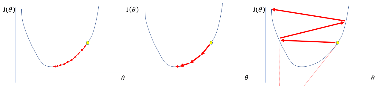
Figure B2 Learning rates that are too small, good, and too large from left to right (after Jordan, 2020).

The activation function adds non-linearity to the network, allowing the model to learn more complex relationships between inputs and outputs (Zheng et al., 2014, June). Each activation function has its advantages and disadvantages, and typical activation functions in deep learning are rectified linear unit (ReLU; Eq. A3), sigmoid (Eq. A4), and hyperbolic tangent (tanh; Eq. A5; Fig. A2; Gu et al., 2018). In deep neural networks, adding more layers with certain activation functions results in the vanishing gradient problem where the gradients of the loss function become almost zero, causing difficulties in training. For instance, the sigmoid function maps a large input space into a small one between 0 and 1. Hence, when the input is very positive or very negative, the sigmoid function saturates (becomes very flat) and becomes insensitive to small changes in its input, causing the derivatives to disappear (Goodfellow et al., 2016). Therefore, in backpropagation, small derivatives are multiplied together, causing the gradient to decrease exponentially, propagating back to the first layer. This causes ineffective updates of weights and biases of the initial layers and consequently inaccuracy. Some solutions to overcome this problem include using specific activation functions like ReLU and tanh and using batch normalization layers to prevent the activation functions from becoming saturated. The ReLU recently gained lots of attention and has been widely used in recent deep learning models (Gamboa, 2017). The advantage of ReLU over sigmoid and tanh is a better generalization, making the training faster and simpler. Hence, we investigated the performance of the model with ReLU, sigmoid, or tanh activation functions in convolutional layers.

$$\begin{array}{}\text{(B1)}& {\displaystyle }\mathrm{ReLU}\left(x\right)=max(\mathrm{0},x)\text{(B2)}& {\displaystyle }\mathrm{Sigmoid}\left(x\right)={\displaystyle \frac{\mathrm{1}}{\mathrm{1}+e^{-x}}}\mathrm{}\mathrm{}\mathrm{}\mathrm{}\mathrm{}\mathrm{}\mathrm{}\text{(B3)}& {\displaystyle }\tanh \left(x\right)={\displaystyle \frac{e^x-e^{-x}}{e^x+e^{-x}}}\end{array}$$

B2 Learning rate

To find the minimum loss function, a move in the negative direction of the gradient is required. This movement is called the “learning rate”, which is the most significant hyperparameter in training a deep neural network. The model error is calculated, and the errors corresponding to weights updated by the learning rate are backpropagated in the network. A learning rate that is too small needs many updates and epochs, reaching the minimum (Fig. A3). On the other hand, a learning rate that is too large causes dramatic updates and leads to oscillations in loss over epochs (Fig. A3). A good learning rate quickly reaches the minimum point between 0.1 and $\mathrm{1}\times {\mathrm{10}}^{-\mathrm{6}}$​​​​​​​ on a log scale.

B3 Padding

The convolution is applied where the input and the filter overlap. Hence, we pad the input by zeros with half the filter size on both sides. Using stride of 1 with “Pads = same” (in Lasagne) in the convolutional 2-D layers results in an output size equal to the input size for each layer.

B4 Activation functions in CN layers

The experiments demonstrate that errors are very high using tanh, whereas ReLU and sigmoid show almost the same performance. As ReLU performs slightly better than sigmoid, we used ReLU in our models.

B5 Dense layer

The dense layers with ReLU functions followed by one dense layer with softmax function are applied after the feature learning and LSTM layers to perform classification. To output the binary classes from the network, softmax or sigmoid functions can be used. We applied softmax as it gives a probability for each class where their total sum is one.

B6 Network optimization

Training CNN involves global optimization by defining a loss function to be minimized over training. For the classification task, the loss function of the models is calculated using categorical cross-entropy between network outputs and targets (Eq. A6), where L is the loss, p is the prediction (probability), t is the target, and c is the number of classes. Then, the mean of the loss is computed over each mini-batch.

$$\begin{array}{}\text{(B4)}& L=-{\sum }_{i=\mathrm{1}}^{c=\mathrm{2}}{t}_i\log \left(p_i\right)\end{array}$$

B7 Update expression

The parameter updating procedure includes feedforwarding, backpropagation, and estimating gradients. The inputs and corresponding targets are iterated in mini-batches for training and validation. Mini-batches split the training data into small batches, which are used during each iteration one after the other to calculate model error and update model parameters. It is computationally efficient not having all training data in memory and model developments, since batch size significantly influences the training time (Fawaz et al., 2019b, July). Mini-batches cause the model to update more frequently, resulting in a more robust convergence and avoiding local minima. There are various algorithms to update the trainable parameters at each mini-batch. We tried the stochastic gradient descent (SGD) with Nesterov momentum, RMSProp, Adadelta, and Adam updates to update the parameters in Lasagne. The SGD with momentum updates the model weights by adding a momentum term so that the overall gradient depends on the current and previous gradients, causing the weights to move in the previous direction without oscillation.

We found that SGD with a momentum term of 0.9 works better than other methods in our cases. The high values for the momentum term result in larger update steps. It is recommended to scale the learning rate by “1 − momentum” for using the high momentum values, which gives 0.1. Interestingly, we already have applied the base learning rate of 0.1 for the LSTM model chosen through trial and error (as explained earlier); however, smaller values are chosen for CNN and CNN-LSTM networks.