Rectification and validation of a daily satellite-derived Antarctic sea ice velocity product

Antarctic sea ice kinematics plays a crucial role in shaping the Southern Ocean climate and ecosystems. Satellite passive-microwave-derived sea ice motion data have been used widely for studying sea ice motion and deformation, and they provide daily global coverage at a relatively low spatial resolution (in the order of 60 km × 60 km). In the Arctic, several validated datasets of satellite observations are available and used to study sea ice kinematics, but far fewer validation studies exist for the Antarctic. Here, we compare the widely used passive-microwave-derived Antarctic sea ice motion product by Kimura et al. (2013) with buoy-derived velocities and interpret the effects of satellite observational configuration on the representation of Antarctic sea ice kinematics. We identify two issues in the Kimura et al. (2013) product: (i) errors in two large triangular areas within the eastern Weddell Sea and western Amundsen Sea relating to an error in the input satellite data composite and (ii) a more subtle error relating to invalid assumptions for the average sensing time of each pixel. Upon rectification of these, performance of the daily composite sea ice motion product is found to be a function of latitude, relating to the number of satellite swaths incorporated (more swaths further south as tracks converge) and the heterogeneity of the underlying satellite signal (brightness temperature here). Daily sea ice motion vectors calculated using ascending- and descending-only satellite tracks (with a true ∼ 24 h timescale) are compared with the widely used combined product (ascending and descending tracks combined together, with an inherent ∼ 39 h timescale). This comparison reveals that kinematic parameters derived from the shorter-timescale velocity datasets are higher in magnitude than the combined dataset, indicating a high degree of sensitivity to observation timescale. We conclude that the new generation of “swath-to-swath” (S2S) sea ice velocity datasets, encompassing a range of observational timescales, is necessary to advance future research into sea ice kinematics.

1 Introduction

Antarctic sea ice plays a central role for Southern Ocean climate and ecosystems. Sea ice is a crucial component in the climate system due to its role in controlling the transfer of energy, gases, and moisture between the polar ocean and atmosphere (Walsh, 1983) and its impact on climate variability through the ice–albedo feedback (Ebert and Curry, 1993) and on deep water formation, as well as fresh water budget by modifying the upper-ocean salinity and density gradient during ice growth and melt (Goosse et al., 1997; Yang and Neelin, 1993). Because of its relatively high albedo compared to open water, especially when covered by snow, sea ice reflects a large portion of the incoming shortwave radiation, thus strongly influencing the Earth's surface energy budget, as well as the atmospheric thermo-circulation (Curry et al., 1995). Furthermore, sea ice production and melt modify the near-surface water; e.g., ice production in coastal polynyas may initiate the formation of dense shelf water, the precursor of Antarctic bottom water, one of the densest water masses in the global circulation (Rintoul et al., 2001). Sea ice also plays an important role in marine ecosystems and biogeochemical cycles as a unique habitat for primary production (Arrigo and Thomas, 2004), and it is affected by a network of complex chemical, biological, and physical interactions (Dieckmann and Hellmer, 2010). Hence, understanding Antarctic sea ice physical processes is critical across many disciplines.

Sea ice kinematics describes sea ice motion and deformation. Accurate characterization of sea ice kinematics is crucial to investigate modifications of the polar sea ice cover and sea ice mass balance (Kwok, 2011). Sea ice motion is driven by external oceanic and atmospheric forcing, as well as internal stresses (Kottmeier and Sellmann, 1996). It is also impacted by physical boundary conditions, e.g., coastline, icebergs, or ice tongues, as well as material properties, e.g., thickness, concentration, and strength (Heil et al., 2011). Sea ice deformation is defined as the spatial gradients in ice velocity driven by winds, currents, and internal stress (Kirwan, 1975; Heil et al., 1998; Marsan et al., 2004). Sea ice deformation may change the drag between ocean and air (Spreen et al., 2017), as well as impacting the distribution of ice thickness and strength (Marsan et al., 2004).

Sea ice kinematics has been studied extensively in the Arctic using satellite observations (e.g., Weiss and Marsan, 2004; Hutchings et al., 2005; Spreen et al., 2017; Hutter et al., 2018). However, satellite-based research of Antarctic sea ice kinematics has been much more limited (Emery et al., 1991; Giles et al., 2011; Hakkinen, 1995; Heil et al., 1998, 2006, 2009; Kimura, 2004; Kimura et al., 2013). In order to characterize Antarctic sea ice kinematics and its effects on physical ice properties accurately, more research on sea ice deformation processes is required (Hutter et al., 2018). With the development of remote sensing technology, satellite observations of Antarctic sea ice motion have been improved in recent years (Spreen et al., 2017; Lavergne et al., 2021). In particular, passive microwave (PM)-derived sea ice motion products give daily, Antarctic-wide coverage with a gridded data format, which may be suitable for characterizing large-scale sea ice kinematics and evaluating basin-scale sea ice simulations (Sumata et al., 2014). However, detailed exploration of this kind of composite satellite observation is required. The spatial resolution of PM-derived sea ice products (25–62.5 km resolution) is relatively low compared to that provided by synthetic aperture radar (SAR) sea ice motion products (150 m resolution for ESA's Sentinal-1A/B), and complete validation of PM-derived motion datasets has yet to be achieved, owing to coastal contamination, numerous missing data, and artifacts, plus limitations in coverage of buoy deployments necessary for complete characterization and validation (Heil et al., 2006; Sumata et al., 2014; Szanyi et al., 2016).

The procedure most widely applied for producing daily sea ice motion vectors is the maximum cross-correlation (MCC) algorithm on satellite-derived daily composites of microwave brightness temperature (T_B) or backscatter coefficient (Ninnis et al., 1986; Emery et al., 1991; Kimura et al., 2013). The MCC method determines the spatial difference between image subsets in two consecutive T_B or backscatter coefficient composite maps by maximizing the cross-correlation coefficient between two composite images of T_B or backscatter coefficient. Sea ice motion products derived from daily-averaged maps of the satellite imagery using the MCC algorithm have been referred to as “daily map” (DM) products (Lavergne et al., 2021). DM products typically have a regular nominal timescale of approximately 1 or 2 d and hence potentially bias the estimated sea ice kinematic parameters by not considering a variety of timescales (Lavergne et al., 2021). Polar orbiting satellite swath convergence means a number of swaths are merged (typically by per pixel mean calculation) to produce composite maps of satellite signals (T_B or radar backscatter), which precipitates a reduction in accuracy of sea ice motion vectors (Lavergne et al., 2021). However, due to the advantages of (a) regular large-scale coverage with a consistent grid, (b) relative ease of calculation, and (c) relative ease of use and interpretation for the dataset end user, DM products have been widely used for recent studies of sea ice kinematics (Szanyi et al., 2016; Hutter et al., 2018). Several PM-derived DM products have been used for investigating sea ice motion in both the Arctic and Antarctic, including the Ocean and Sea Ice Satellite Application Facility (OSI SAF) sea ice drift product OSI-405-c (Lavergne, 2016), henceforth referred to as the OSI SAF product; the NASA Polar Pathfinder Daily 25 km Equal-Area Scalable Earth Grid (EASE-Grid) Sea Ice Motion Vectors product (Tschudi et al., 2020) from the National Snow and Ice Data Center (NSIDC), henceforth referred to as the NSIDC product; and the daily sea ice motion product produced by Kimura et al. (2013), henceforth referred to as the KIMURA product.

Daily input data of the KIMURA product include both the horizontal and vertical polarization channel T_B images for both ascending (ASC) and descending (DES) orbital sections (i.e., four independent images) from the NASA's Advanced Microwave Scanning Radiometer – Earth Observing System (AMSR-E) and Advanced Microwave Scanning Radiometer 2 (AMSR2), on the sun-synchronous Global Change Observation Mission – Water 1 (GCOM-W1) platform. The final KIMURA daily sea ice velocity product is then derived as the mean value of these four datasets. AMSR2, used by the KIMURA product after 2012, passes over each observed point on the Earth surface at approximately the same local (solar) time, and for any given pixel, the sensing times for ASC and DES passes differ. The local overpass time of the ASC pass in the Antarctic sea ice zone (i.e., ∼ 60^∘ to 78^∘ S) is around 15:00 local time (Fig. 1, red bar), and the DES pass is around local midnight (Fig. 1, blue bar). At higher latitudes where several adjacent swaths observe the same pixel, the local times of observation for these several swaths are centered around the nominal overpass time but offset by several orbital periods (i.e., offset from the nominal local time by $\pm n\times \mathrm{98}$ min, where n can be 1, 2, or more depending on latitude). The daily combined KIMURA sea ice motion product (represented by the green bar in Fig. 1) is the mean of the ASC and DES data. As such, it has a true (nominal) time base of approximately 39 h. This exceeds that of the ASC and DES motion products (which have a nominal time base of 24 h). Previous buoy-based research demonstrated that shorter-timescale observations can represent sea ice motion and kinematic parameters with higher magnitude than longer-timescale observations (Hoeber and Gube-Lenhardt, 1987; Heil and Allison, 1999), but analogous research for satellite-based observational datasets is quite limited. We postulate that a shorter-timescale sea ice motion dataset (i.e., derived from ASC or DES DM composites, with their inherent ∼ 24 h timescale) will result in higher estimates of the kinematic parameter magnitude compared to a longer-timescale dataset (i.e., a product combining ASC and DES data). Thus, to investigate the influence of the timescale on the accuracy of the PM-derived sea ice motion and derived kinematic parameter magnitude, individual ASC and DES KIMURA datasets are generated and investigated here.

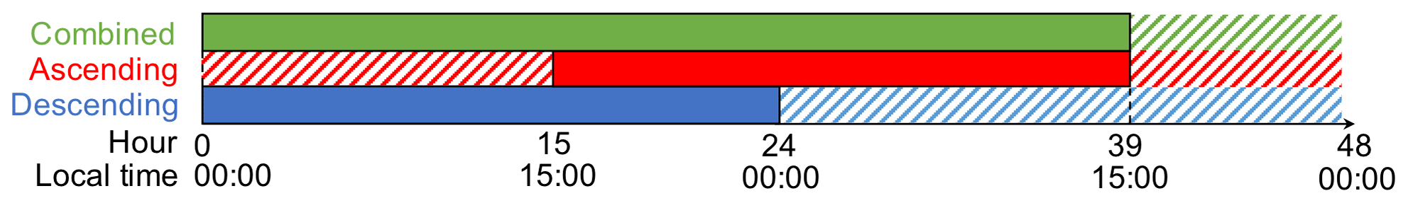
Figure 1 Representation of the timescale of the combined (ASC and DES averaged together) KIMURA daily sea ice motion product, as well as the timescales of ASC and DES components.

Recently sea ice motion has been estimated from PM-derived T_B partial-overlap swath pairs from a wide range of temporal baselines (from one orbit of ∼ 90 min to 3 d). This approach is referred as “swath-to-swath” (S2S) (Lavergne et al., 2021). For S2S, the time base for derived motion is a function of the temporal separation of individual swaths in each pair and hence differs between pairs (Lavergne et al., 2021). As such, the raw S2S-derived motion swaths do not constitute a regular, full-coverage time series. However, since S2S most accurately provides ice motion from individual swaths across a range of time bases, Lavergne et al. (2021) concluded that sea ice motion based on S2S is more accurate than that from DM.

We hypothesize that a greater number of satellite swaths used for averaged maps of satellite signals (e.g., T_B DMs) may negatively impact the performance of PM-derived sea ice motion vectors. Here, we investigate this hypothesis by performing comparisons against drifting buoy-derived motion in different latitude ranges with the expectation that the DM-based KIMURA product performs better at lower latitudes, where swath overlap averaging is lower. We note that the OSI SAF sea ice motion product is derived by averaging over 2 d to increase the signal-to-noise ratio (SNR) of this operational product (Lavergne, 2016). This extended averaging interval arises, in part, due to OSI SAF integrating multiple sensors. Because of the extended time base of the OSI SAF product, direct comparison with the NSIDC and KIMURA product in a kinematic parameter context is not possible. Hence the OSI SAF dataset is not considered further in this study, although implications of a longer temporal baseline are considered in the discussion. Version 3 of the NSIDC dataset is known to display a high degree of autocorrelation in neighboring vectors (Szanyi et al., 2016) which would be detrimental to the derivation of kinematic parameters. Version 4 of the NSIDC product has reduced this autocorrelation to some extent (Tschudi et al., 2020); however this product still assimilates from several instruments, so retrieval of kinematic parameters will suffer from cross-instrument averaging. Furthermore, as the NSIDC product does not use AMSR2, spatial resolution is inherently lower than the KIMURA product. For these reasons, the NSIDC dataset is not considered further here. A comparison of the KIMURA, OSI SAF, and NSIDC sea ice motion products against buoy observations is provided in Appendix A. The KIMURA product is the only PM-derived dataset we consider here; it provides daily gridded sea ice motion vectors of the complete Southern Ocean at 60 km horizontal resolution.

The objectives of this study are to (a) evaluate the KIMURA ice motion product separately for the ASC, DES, and combined datasets by comparison with coincident drifting buoy-derived velocities and (b) investigate impacts of the observational timescale of the ice motion products on a representation of Antarctic sea ice kinematic magnitude. This study will provide characterization of the satellite sensor configuration and observational timescale on the accuracy of derived sea ice motion, as well as the ability to represent Antarctic sea ice kinematic parameters.

2 Datasets

2.1 PM-derived sea ice motion

The KIMURA sea ice motion products (Kimura et al., 2013) used here were produced at 60 km × 60 km resolution on a regular 145 × 145 pixel grid covering the entire Southern Ocean with daily data from 23 June 2012 to 1 June 2020. These were calculated by applying the MCC method to 36.5 GHz, 10 km resolution AMSR2 T_B images (both vertical and horizontal polarization, ASC, and DES) from the Arctic Data Archive System (ADS) of the Japanese National Institute of Polar Research (NIPR). The MCC method determines the spatial offset that maximizes the cross-correlation coefficient between two T_B arrays (at a resolution of 10 km per pixel) in consecutive images (from an ASC observation to the next ASC observation, or DES to DES). For this procedure, 6 × 6 grid cell (60 km × 60 km) arrays are utilized. At first, an ice motion vector quantized to an integer number of grid intervals (10 km) is computed. Then detections of false cross-correlation matches are automatically filtered out by the following procedure: (1) eliminate vectors with a correlation coefficient of less than 0.5 of the MCC coefficient; (2) retain the “reliable” vectors with more than 0.78 of the correlation coefficient, i.e., within the 95 % confidence interval; and (3) vectors with a correlation coefficient of between 0.5 and 0.78 of the MCC coefficient are eliminated if they differ from the “reliable” vectors (within a search radius of 100 km) by more than 23 cm s⁻¹ (i.e., 2 px d⁻¹). Finally, filtered sea ice motion vectors, on a 10 km × 10 km grid, are organized into a 60 km × 60 km resolution dataset. In this procedure, at least six vectors are utilized for each resulting vector. If the number of the available vectors is less than six, that grid is regarded as missing data. The final KIMURA combined daily dataset is calculated as the mean value of four datasets derived from the horizontal and vertical polarization channel images from ASC and DES satellite passes. By combining the ASC and DES passes in this fashion, the true characteristic timescale becomes approximate 39 h, as described in Fig. 1. In this work, we also produce and analyze daily sea ice motion vectors computed for the shorter-timescale (true 24 h) ASC and DES swath composites.

2.2 In situ buoy-derived sea ice motion

Velocities derived from buoy positions are suitable for validating satellite-derived sea ice motion (Hoeber and Gube-Lenhardt, 1987; Heil and Allison, 1999). Here we evaluate the three KIMURA datasets using three buoys deployed on ice floes in the Weddell and Ross seas (Table 1 and Fig. 2). These have been named the southern Weddell Sea buoy (Fig. 2, red), the central Weddell Sea buoy (Fig. 2, green), and the Ross Sea buoy (Fig. 2, orange). In the Weddell Sea, several drifting sea ice buoys were deployed in 2018 (Schröder, 2018). Only two of these are analyzed in this paper as the buoys were deployed in meso-scale arrays, hence at sub-grid scale to the KIMURA data. Others in this deployment were near the coast where the KIMURA ice motion product suffers from coastal contamination. Raw positions were quality-controlled, and any erroneous data were removed. A weighted polynomial interpolator (Scargle, 1982; Heil et al., 2001) was applied to the quality-controlled position measurements to yield an equi-temporal hourly time series. In the Ross Sea, a total of eight position-only buoys were deployed as part of the Polynyas, Ice Production, and seasonal Evolution in the Ross Sea (PIPERS) cruise during austral autumn of 2017 (Tison et al., 2020). Four were excluded due to coastal proximity and another one due to a short time series. Here we analyze only one of the three remaining buoys as they shared similar trajectories.

Table 1 Buoy deployment information.

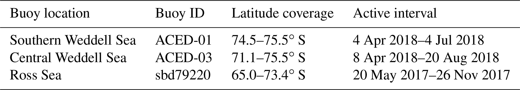
Figure 2 Mean daily number of AMSR2 swaths for (a) ASC and (b) DES passes. Trajectories of three buoys used in this study are also shown.

3 Methods

3.1 Validation of KIMURA-derived ice motion datasets using buoy data

To evaluate the skill of the three KIMURA datasets to represent sea ice motion, we compare these with buoy-derived sea ice velocity using three validation metrics: Pearson's correlation coefficient, regression slope, and root mean square (RMS) deviation (RMSD). Since AMSR2 is in a sun-synchronous orbit, it passes over each point on the Earth at roughly the same local (solar) time. For daily motion comparison buoy time stamps, referenced in UTC time, are converted to local (solar) time to investigate the start and end time for daily motion comparison. To calculate daily buoy velocity, a 24 h interval of buoy positions is selected to coincide with the satellite overpass time. The choice of the start time for a 24 h interval is informed by calculating all validation metrics in hourly intervals from −48 h (local midnight of 2 d before) to +48 h (local midnight of 2 d later). The ASC, DES, and combined start times which are found to maximize the correlation between KIMURA and buoy sea ice velocity were fixed for all analyses. Spatially, KIMURA pixels contributing to the daily velocity were selected by weighting the velocity in the pixels that the buoy passed through in the preceding 24 h.

We note that the number of AMSR2 swaths (Fig. 2, blue shading) increases rapidly poleward of 74^∘ S for both ASC and DES passes. This is particularly evident in the ASC case, in which a strong discontinuity is observed at this latitude owing to the oblique, forward-looking viewing geometry of the instrument. In both ASC and DES cases, more satellite swaths will be merged together at higher latitude (i.e., a higher degree of temporal “smearing” is expected at higher latitudes, with potential detriment to derived motion products). By extension, fewer swaths will be merged at lower latitudes (i.e., at northern extremes, the DM product tends toward the S2S product, with reduced temporal smearing). Based on the results of Lavergne et al. (2021), we expect better performance of the KIMURA product at lower latitudes for this reason. To investigate the effect of compositing more satellite swaths on the accuracy of the KIMURA product, buoy comparisons are separated based on their latitude (Table 1). We separate the central Weddell Sea buoy to four 1^∘ latitude segments and the Ross Sea buoy to four 2^∘ latitude segments to support this analysis (the southern Weddell Sea buoy has insufficient latitudinal range for this analysis).

3.2 Calculation of sea ice divergence

Various differential kinematic parameters (DKPs) are frequently used to represent sea ice kinematics (Molinari and Kirwan, 1975; Hutchings et al., 2012): divergence (D), shear deformation rate (pure shear), normal deformation rate (stretching), and vorticity (rotation). Here we use D to investigate a hypothesized increase in DKP magnitude when considering the shorter-timescale (24 h) ASC and DES datasets, compared to the combined dataset. To generate daily maps of D from the KIMURA product, D at the center of four neighboring pixels was calculated as follows:

$$\begin{array}{}\text{(1)}& D={\displaystyle \frac{\partial u}{\partial x}}+{\displaystyle \frac{\partial v}{\partial y}},\end{array}$$

where u and v are daily sea ice velocities in the eastward and northward directions, respectively, while x and y represent eastward and northward components. We evaluate the magnitude of D for the combined, ASC, and DES datasets by computing the monthly RMS deviation (hereafter RMSD, i.e., a measure of monthly variability). Variability in D over a period of 1 month is used here to assess the relative magnitude of the DKPs. Furthermore, based on the latitude hypothesis that more satellite swaths become merged causing more smoothing at higher latitudes, we also expect that D RMSD will decrease from north to south.

4 Results

4.1 KIMURA data assessment

Here, we validate the three KIMURA sea ice motion datasets using daily velocity from buoys in the Ross and Weddell seas. First, we report some problems discovered in the KIMURA datasets.

4.1.1 Problem 1: triangular regions with persistent low velocity

Initial inspection of the KIMURA product reveals the existence of two triangular regions with recurring low velocity (every second day). These are in the western Amundsen Sea for the ASC dataset (triangular region in Fig. 3a) and the Weddell Sea for the DES dataset (triangular region in Fig. 3c). These problem regions are also evident in the combined product, although their impact is masked (halved) due to the averaging of ASC and DES velocities. Upon investigation, this occurs at an acquisition time of around midnight UTC, in which swath duplication has erroneously occurred in the T_B DM product (from NIPR and ADS). Such areas with replicated values in the source T_B images manifest as areas of near-zero velocity in the KIMURA product. To rectify this problem, we produced a new version of the KIMURA product using 10 km resolution AMSR2 Level-3 36.5 GHz T_B images from the Japan Aerospace Exploration Agency (JAXA) ASC and DES T_B daily composites which do not exhibit erroneous swath duplication. A new combined product is produced as the mean of these two with the same 60 km horizontal grid resolution. Rectified KIMURA velocity maps (Fig. 3b and d) reveal that this problem has been overcome. We note that the sea ice velocity in other regions changes slightly, which is due to small differences between the NIPR and JAXA T_B DM composites, but investigation is beyond the scope of this work.

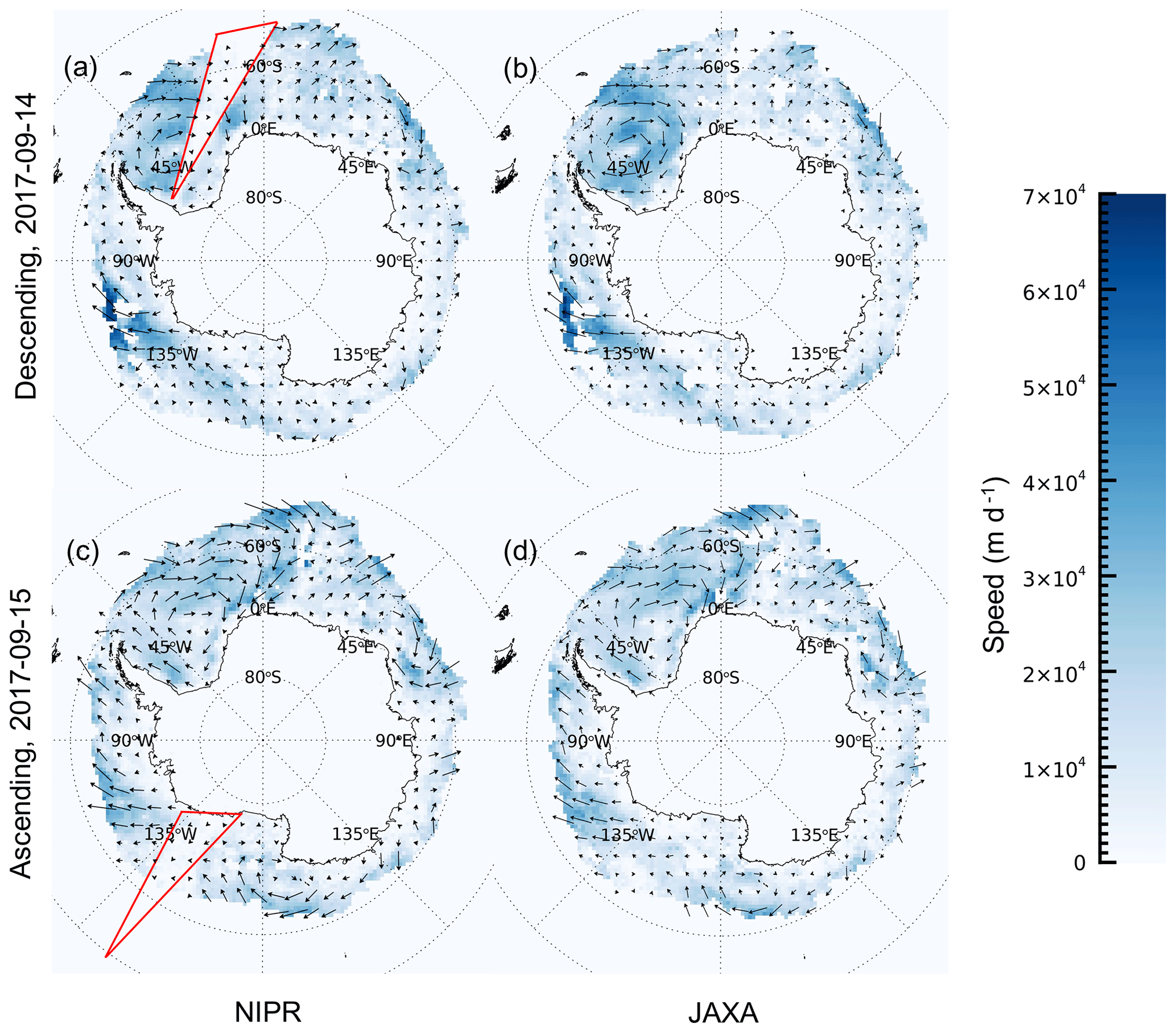
Figure 3 Sea ice speed (color scale) and velocity (vectors) from (a) the original KIMURA DES dataset (produced from the NIPR T_B composite) and (b) the rectified KIMURA DES dataset (produced from JAXA T_B composite) on 14 September 2017. Panels (c) and (d): same as for (a) and (b) but for the ASC dataset on 15 September 2017. Vectors are subsampled by a factor of 5 to enhance visibility. Red triangular areas shown in (a) and (c) mark the regions of erroneously low velocity.

4.1.2 Problem 2: incorrect assumption of 24 h time separation

The work described above revealed a second problem with the KIMURA product: an interval of exactly 24 h time separation between consecutive T_B composites was assumed, which is rarely correct. We analyze actual time separation between each data pair collected on contiguous days. In order to characterize the variability in time separation, we calculate the standard deviation of time separation for both ASC and DES datasets. The result for September 2017 is displayed in Fig. 4 (all months similar, not shown here).

The mean time separation is close to 24 h throughout each month; however there is a region of high standard deviation around midnight UTC, which occurs in the Amundsen Sea for the ASC swaths (Fig. 4a) and the eastern Weddell Sea for the DES swaths (Fig. 4b). This indicates that the actual time separation of pixels in subsequent daily composites can regularly be up to 34 h or as low as 14 h in these two areas. Thus, the resulting velocity is regularly incorrect by up to 40 %, and the combined KIMURA dataset exhibits errors for these locations. However, any error is compensated for by the following day's velocity field since the time intervals oscillate around 24 h. As such, it will not have a strong effect on long-term sea ice motion, but it is highly detrimental when deriving sea ice kinematic parameters. To fix this problem, the actual time separation needs to be taken into account when producing daily sea ice velocity of KIMURA ASC, DES, and combined datasets. The appropriate correction has been performed for all remaining analyses presented here.

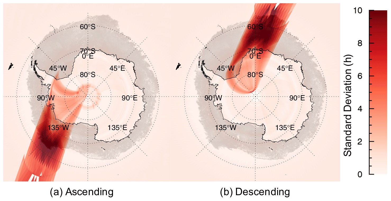
Figure 4 Standard deviation of time separation for AMSR2 (a) ASC and (b) DES datasets in September 2017. The shaded background represents AMSR2-derived sea ice concentration on 1 September 2017 (Melsheimer and Spreen, 2019).

In summary, two problems have been discovered in the original KIMURA product which have been rectified in all KIMURA data used in this study. Henceforth, the corrected KIMURA product is referred to as the KIMURA_new product. The official release of the rectified KIMURA sea ice motion is a work in progress.

4.2 Validation of KIMURA_new product

The KIMURA_new product is compared to buoy-derived sea ice motion. The buoy start and end times needed to maximize correlation coincide exactly with the local (solar) times of corresponding satellite passes, i.e., 15:00, 00:00, and 08:00 UTC for ASC, DES, and combined data, respectively, giving confidence in our methodology. Validation metrics are given in Table 2.

Table 2 Comparison between KIMURA_new dataset and buoys.

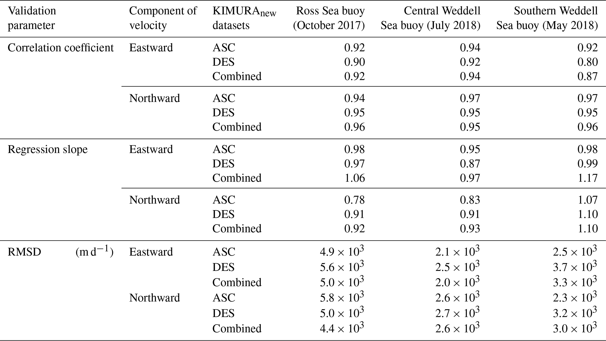
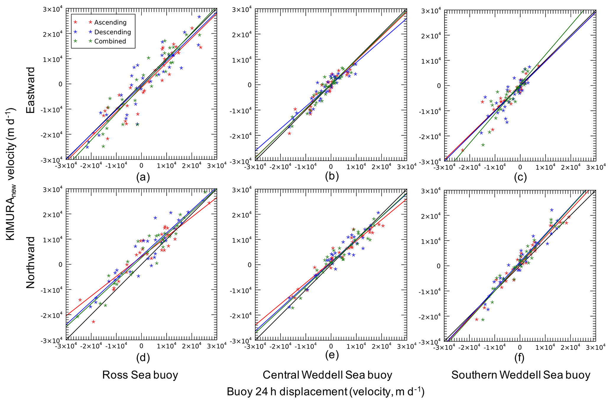
Figure 5 Scatterplot of comparisons between KIMURA_new dataset (ASC is red, DES is blue, and combined is green) and buoy velocities (24 h displacement) in eastward (a, b, and c) and northward (d, e, and f) directions in October 2017 for the Ross Sea buoy, July 2018 for central Weddell Sea buoy, and May 2018 for southern Weddell Sea buoy. The solid black line represents the regression slope of 1.0.

The validation metrics (Table 2) demonstrate that the KIMURA_new dataset represents buoy velocities well. The mean value of the correlation coefficient of comparison between three KIMURA_new datasets and three buoys is 0.93, and the mean of the regression slope is 0.97. The monthly average sea ice motion speed is around 15.8 km d⁻¹ for Ross Sea in October 2017, 9.7 km d⁻¹ for central Weddell Sea in July 2018, and 8.3 km d⁻¹ for southern Weddell Sea in May 2018. We notice that the comparison of KIMURA_new with the Ross Sea buoy (Table 2) exhibits relatively large RMSD (from 4.4 to 5.8 km d⁻¹), considerably larger than that of the two Weddell Sea buoys (from 2.0 to 3.7 km d⁻¹), as well as larger than the validation of DM-derived sea ice motion RMSD (from 2.3 to 2.9 km d⁻¹) from Lavergne et al. (2021). The comparisons between KIMURA_new and buoys (Fig. 5) confirm this for sea ice in the Weddell Sea. Here the regression slopes converge to 1.0, and points lie closer to the regression lines than for the Ross Sea comparison.This difference in RMSD prompted further investigation into the performance difference between the Ross and Weddell seas. Since the MCC algorithm requires discernible structure in the underlying T_B imagery to produce accurate vectors, we suggest this RMSD discrepancy is caused by a differing degree of heterogeneity of T_B between the Ross Sea and Weddell Sea ice during these buoy deployments. To investigate why the RMSD of the Ross Sea result is higher than that of the Weddell Sea, we analyze the spatial standard deviation of 36.5 GHz, 10 km vertically and horizontally polarized T_B (i.e., the input data to the MCC algorithm) in limited areas around both buoy deployments.

Figure 6 ASC and horizontally polarized daily T_B composite acquired on 1 July 2018. Buoy trajectories are indicated by black lines in the Weddell and Ross seas. Square black boxes display the locations of subsets centered around the central Weddell Sea and Ross Sea buoys analyzed in Table 3.

Table 3 Standard deviation of T_B for subregions in the Weddell Sea and Ross Sea shown in Fig. 6. Time periods are the corresponding time of buoys within these subregions. Satellite orbits and polarizations are ASC horizontal (ASC, H), ASC vertical (ASC, V), DES horizontal (DES, H), and DES vertical (DES, V).

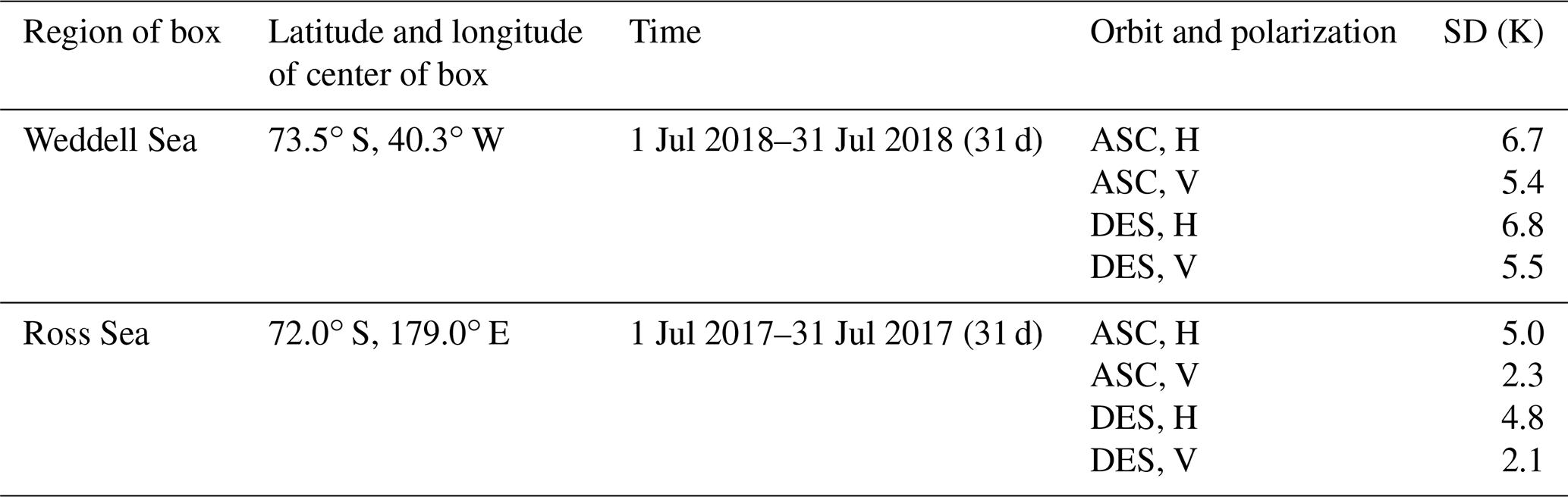
Firstly, we select subregions of 31 × 31 T_B pixels (i.e., 310 km × 310 km) that cover the buoy areas of the Ross and Weddell seas (Fig. 6). Then we compute the standard deviation within each subregion using all data, while the buoys remain within the subregion, as well as for all four combinations of satellite orbital section and polarization. The standard deviation of T_B in the Ross Sea is lower than the Weddell Sea in all satellite orbital sections and polarizations, with a mean of 3.6 K for Ross Sea and 6.1 K for the Weddell Sea. This indicates that the spatial variability in T_B within the sea ice of the Ross Sea is lower than that of the Weddell Sea (for these cases). The relative homogeneity in the underlying T_B data in the western Ross Sea, a region dominated by new ice formed in the Ross Ice Shelf and Terra Nova Bay polynyas, reduces the ability of the MCC to retrieve accurate sea ice motion due to less discernible structure in the underlying T_B imagery (in agreement with Meier et al., 2000, who found that errors are maximized in regions of new ice).

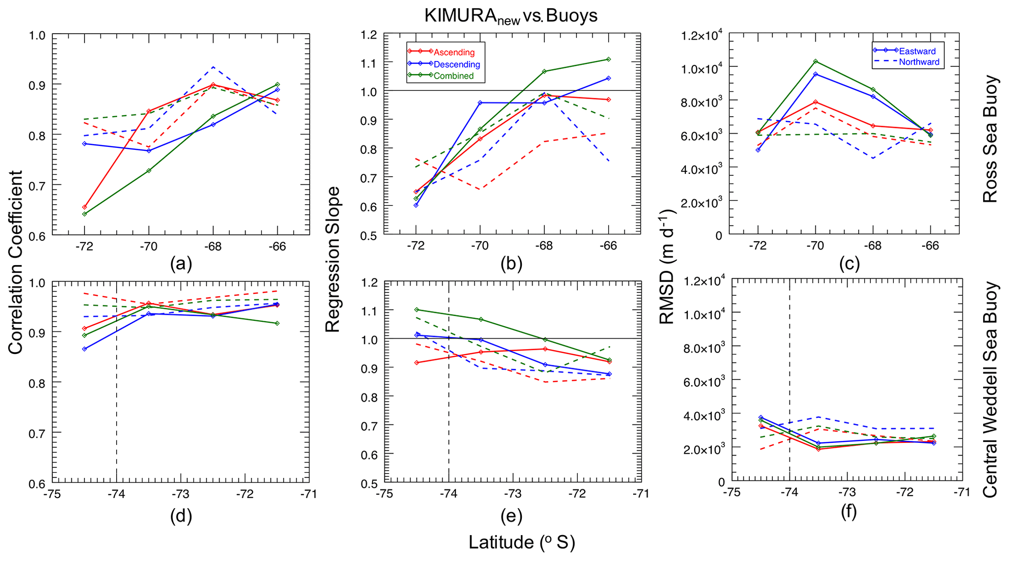
Figure 7 Comparison between KIMURA_new dataset (ASC is red, DES is blue, and combined is green) and buoy velocity using (a, d) correlation coefficient, (b, e) regression slope, and (c, f) RMSD. Vertical dashed lines in the central Weddell Sea panels (lower row) mark the latitude of the AMSR2 swath discontinuity (74^∘ S) shown in Fig. 2.

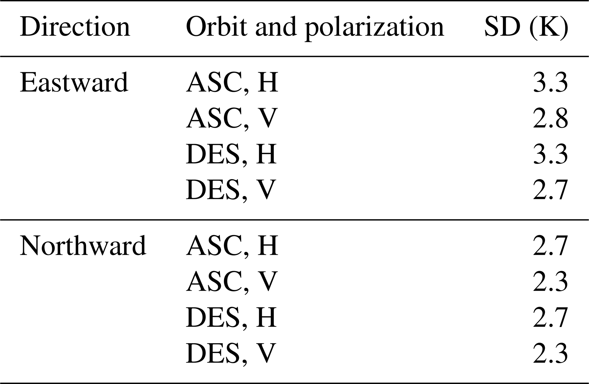
To investigate the hypothesis that DM-based daily sea ice motion vector performance is latitude-dependent, we calculate the three validation metrics in different latitude ranges along the buoy trajectories (Fig. 7). The southern Weddell Sea buoy is excluded from this analysis due to insufficient latitudinal range. We find that the validation metrics for both remaining buoys generally improve as they move further north (Fig. 7). For the central Weddell Sea buoy comparison, eastward velocity results (Fig. 7 lower row, solid lines) improve from south to north across the swath number discontinuity (74^∘ S), confirming our hypothesis that regions with fewer satellite swaths may yield improved performance for DM-based sea ice motion retrieval. However, northward ice velocity results in the central Weddell Sea case (dashed lines) exhibit a slight RMSD (Fig. 7f) deterioration from south to north. We attribute this unexpected deterioration to anisotropic T_B heterogeneity, noting that the heterogeneity in the northward component is lower than that in the eastward component (shown in Table 4), giving higher confidence in the result of the eastward component and underscoring the importance of heterogeneous imagery when using the MCC algorithm.

Table 4 Eastward and northward components of standard deviation of T_B images in the subregion of the central Weddell Sea buoy from July 2018, corresponding to the time the buoy resided within the black box (Fig. 6). Satellite orbits and polarizations are ASC horizontal (ASC, H), ASC vertical (ASC, V), DES horizontal (DES, H), and DES vertical (DES, V).

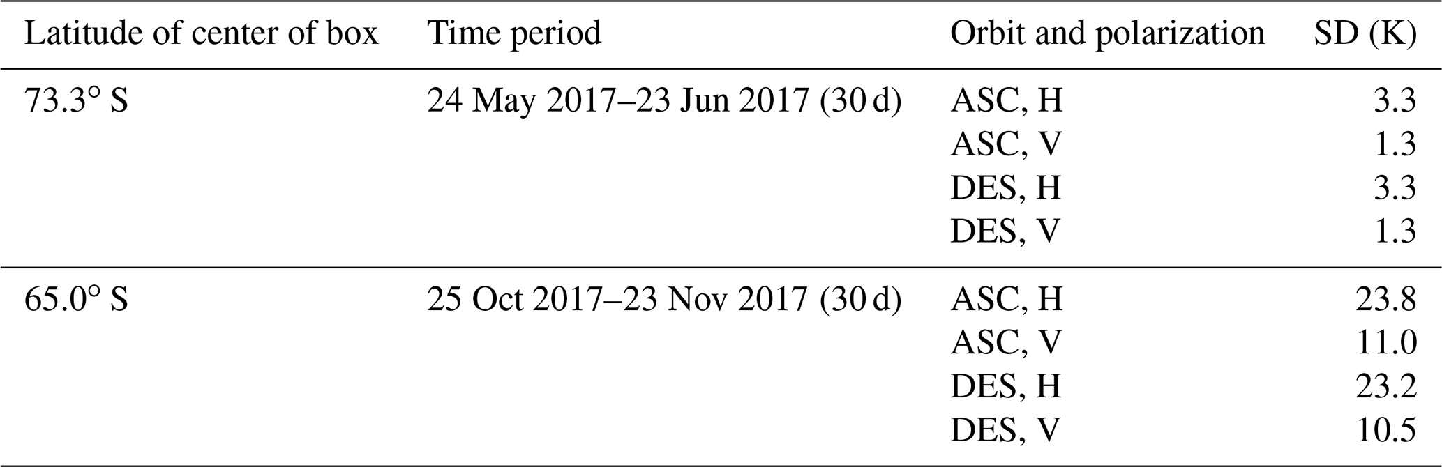
The validation of the Ross Sea buoy (Fig. 7, upper row) indicates that both the eastward and northward performances improve progressively from south to north. The entire Ross Sea buoy trajectory is located to the north of the swath number discontinuity (i.e., in the relatively low swath number regime, as indicated in Fig. 2), so we suppose that the gradual satellite swath decreases from south to north are not the key reason of the increasing accuracy of the KIMURA_new product here. Based on our findings about the importance of underlying image heterogeneity, we expect that there may be a higher degree of T_B homogeneity to the south, whereas in the north, approaching the ice edge, lower and patchier sea ice concentration produces relatively high heterogeneity (giving many features for the MCC algorithm to track). In order to represent and analyze the image homogeneity for the southern and northern parts of the Ross Sea buoy trajectory, we examine the standard deviation of T_B images in two 20 × 20 pixel subsets to approximately match the 2^∘ latitude bin used in computing the validation metrics at the southern and northern ends of its trajectory (Fig. 8). We find that the standard deviation of T_B in the southern box is much lower than in the northern box, with a mean of 2.3 K for the southern box and 17.0 K for the northern box of the Ross Sea buoy (Table 5). This analysis indicates that T_B in the northern part of the Ross Sea buoy trajectory exhibits more structure than in the southern part. Thus, we conclude that the performance of MCC-based sea ice motion algorithms is sensitive to structure in the underlying T_B imagery, with potential regional ramifications which are considered in the discussion.

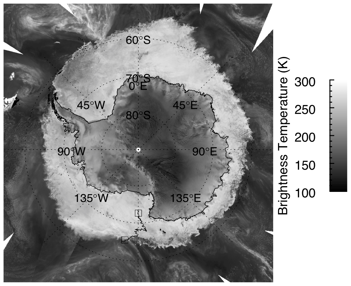
Figure 8 Map of ASC horizontal T_B image on 13 September 2017. Black trajectory and square boxes display subsets at start and end of the Ross Sea buoy.

Table 5 Standard deviation of T_B images in two subregions along the Ross Sea buoy trajectory. Times correspond to the buoy within each box. Satellite orbits and polarizations are ASC horizontal (ASC, H), ASC vertical (ASC, V), DES horizontal (DES, H), and DES vertical (DES, V).

The three buoys used in this study were all deployed during Antarctic winter when the sea ice south of the marginal ice zone is relatively dry. A follow-up summertime comparison would provide important information regarding the performance of the KIMURA_new product during the sea ice melt season, when the microwave emissivity contrast is reduced, potentially giving a more homogeneous T_B field near the ice edge and reducing the performance of this technique.

4.3 KIMURA_new-derived sea ice deformation

Accurate sea ice motion data are crucial for the calculation of sea ice kinematic parameters. Here we investigate the effect of using the shorter-timescale ASC and DES sea ice motion products to retrieve sea ice D and compare it to those derived from the longer-timescale combined product.

4.3.1 Sea ice divergence

Figure 9 illustrates per pixel D RMSD for the month of July 2017 derived from the KIMURA_new ASC, DES, and combined datasets. The spatial mean circumpolar D RMSD (Fig. 9) for the combined dataset (1.08 × 10⁻⁶ s⁻¹) is lower in magnitude than that of both the ASC (1.31 × 10⁻⁶ s⁻¹) and DES datasets (1.22 × 10⁻⁶ s⁻¹), indicating that the ASC and DES datasets can represent a higher magnitude of differential sea ice motion than the combined dataset. The magnitude of derived sea ice kinematics is demonstrated to be sensitive to timescale, and we have shown that shorter-timescale input data produces higher sea ice D values.

To investigate the impacts of swath number on representing sea ice D magnitude, we compare the July 2017 mean D RMSD calculated by KIMURA_new ASC, DES, and combined datasets in subregions north and south of the swath number discontinuity (74^∘ S for both ASC and DES; Fig. 2). The mean D RMSD at higher latitudes is about 9 %, 14 %, and 16 % lower than at lower latitudes (i.e., north of 74^∘ S) for the ASC, DES, and combined datasets, respectively. This indicates that DM-estimated sea ice D RMSDs are lower at higher latitudes potentially due to a greater degree of smoothing due to more merged swaths at higher latitudes, i.e., an undesirable bias may be introduced as a consequence of the observation configuration. While we have not investigated physical sea ice properties, which may also give rise to the lower DKP magnitude south of the swath discontinuity, we note that in the major Southern Ocean basins sea ice might be thinner and mechanically weaker at higher southern latitudes than that further north since much of it has formed recently in coastal polynyas (particularly in the southwestern Ross and Weddell seas). As such, we would expect a greater magnitude of sea ice D variability there. In this case, using an S2S dataset to derive sea ice motion may be required to remove observational bias.

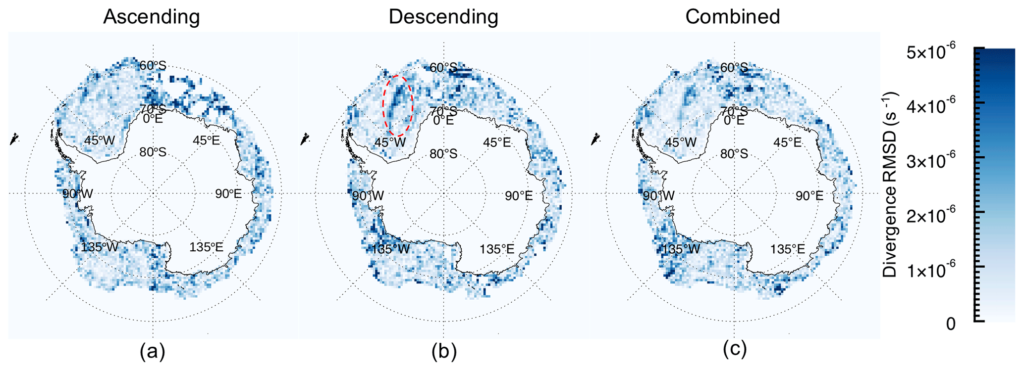
Figure 9 Mean D RMSD for (a) ASC, (b) DES, and (c) combined KIMURA_new datasets of July 2017. The dashed red ellipse highlights the high D RMSD filamentary structure in the DES map, described in the text.

Figure 9 also indicates that there are several regions with distinct features when using ASC and DES sea ice motion to calculate D. However, the central northern Weddell Sea stands out, exhibiting a region of high D RMSD in the DES (Fig. 9b, dashed red circle), which is not mirrored in the ASC RMSD D map. Such filamentary structures exist in the Weddell Sea during most wintertime months (not shown) and occur in ASC and DES maps equally, but the location is non-stationary. Given the non-stationary nature of this signal, we suggest that it is not an artifact of the satellite or analysis procedure. Noting the sun-synchronous observation platform, we suppose that this filamentary structure might be a response to external (oceanic or atmospheric) forcing with a ∼ 24 h period, such as tidal currents or near-surface wind stress, but further research is beyond the scope of this paper. That this structure is (a) not present in the ASC map and (b) muted in the combined map underscores the importance of considering observational timescale and overpass time when interpreting maps of DKPs.

5 Discussion

In this study, we firstly analyze DM-based Antarctic sea ice motion retrieval on sea ice kinematics by separating PM-derived KIMURA_new sea ice motion product into ASC and DES. Results show that the performance of KIMURA_new datasets is a function of latitude and that the timescale of the composite dataset has crucial influence on retrieved sea ice kinematic magnitude. Here, we discuss the impacts of features of the satellite observational configuration on sea ice kinematic representation and how to improve observations in the future.

5.1 Impact of features of satellite observational dataset on kinematic representation

We find a strong link between the heterogeneity of underlying satellite-derived maps (i.e., T_B in this study) and the performance of the satellite-derived sea ice velocity dataset when using the MCC algorithm. From the results shown in Table 4, the Weddell Sea T_B composite presents as a relatively heterogeneous T_B field, giving better performance of sea ice velocity vectors compared to the Ross Sea comparison (Sect. 4.2). There is a higher degree of homogeneity in the southern and central Ross Sea than in the northern Ross Sea, and validation metrics (Fig. 7a and b) consequently improve to the north (Sect. 4.2). The KIMURA_new product is derived from both horizontal and vertical polarizations, and T_B heterogeneity for horizontal polarization is found here to be generally higher than that for vertical polarization T_B (Tables 3, 4, and 5) likely because the difference between emissivity of the first-year sea ice and open ocean at 36.5 GHz is significantly larger for horizontal polarization than for vertical polarization (Mathew et al., 2009). Thus, we expect that sea ice velocity only derived by horizontal polarization, instead of using both polarizations, may be useful when more accurate characterization of kinematics is desired.

Higher-spatial-resolution imagery may also be advantageous in terms of providing underlying imagery which is relatively heterogeneous (i.e., improving MCC algorithm performance). In addition to the results shown in Table 2 (showing a high RMSD in the Ross Sea buoy validation metrics), we also investigate the standard deviation of T_B in the Ross Sea for several other months in 2017 and 2018 (not shown here) and find that the relatively homogeneous 36.5 GHz T_B in the Ross Sea is likely to be a persistent feature of ice in this sector. Also, other parameters of satellite signals, such as radar backscattering cross section, may provide more independent structure for the MCC algorithm and may be more successful in a S2S framework than DM. For this reason, the inclusion of scatterometer data may give rise to the good performance of the OSI SAF sea ice drift product OSI-405 (Lavergne, 2016), albeit giving a (often undesirable) longer timescale due to the inclusion of several instruments. Also, we suggest that all MCC-based sea ice motion products report cross-correlation signal-to-noise ratio as an objective measure of vector confidence and uniqueness of matching (i.e., as a metric for heterogeneity within the MCC search window; Altena et al., 2021).

Here we suggest that DM-derived kinematic maps represent not only sea ice kinematics but also features of the orbit, which is highly undesirable. However, the underlying sea ice motion datasets are still valuable for studies on bulk ice export/flux (e.g., Drucker et al., 2011), which favor low RMSD datasets assimilating data from many instruments with temporal baseline a secondary consideration. In this case, the satellite motion datasets based on DM techniques (including the KIMURA product) are still valuable (e.g., Drucker et al., 2011). When vector quality is paramount, inclusion of multiple instruments is important. Both S2S and DM products using scatterometer data in addition to radiometers (e.g., the OSI SAF product) would benefit from the inclusion of higher-resolution scatterometer data (e.g., Lindsley and Long, 2010).

A recent study by Lavergne et al. (2021) shows that an S2S sea ice motion dataset provides a diverse set of temporal baselines from which more rigorous gage kinematic processes can be derived over a range of timescales. However, interpretation of an S2S product, with its inherently irregular temporal grid and spatial coverage, is likely to be more difficult than a DM-derived product. Even when using only a single instrument, DM-derived datasets with their inherently long, low-diversity timescale cannot track sea ice deformation processes to the same degree as S2S products. Thus, looking to the future of sea ice kinematic studies, a dataset with the flexibility to provide a wide range of timescales is necessary.

5.2 Future development of ice kinematic representation

To fully and accurately represent sea ice kinematics, some avenues for targeted research pathways are suggested here. From recent research, S2S-derived sea ice trajectories obtained from AMSR2 imagery have been found to be more accurate than the DM-derived equivalents (Lavergne et al., 2021). However, S2S products give better coverage of sea ice motion datasets in the Arctic compared to the Antarctic due to Antarctic sea ice existing at lower latitudes. Thus, combining DM and S2S concepts together and producing a mixed dataset that takes advantage of both approaches is recommended for improvement in ice kinematic representation in the future while maintaining ease of use for end users.

More satellites and instruments are needed to acquire more frequent swaths and obtain a more comprehensive sea ice motion dataset, as well as to provide a wider diversity of overpass times to avoid the problem of aliasing shown in Fig. 9. For example, two satellites in a tandem configuration might produce a 12 h timescale DM product rather than the 24 h timescale available from a single platform.

Recently, Lavergne et al. (2021) discussed the Copernicus Imaging Microwave Radiometer (CIMR) mission for both the Arctic and Antarctica. CIMR will be a conically scanning sun-synchronous microwave radiometer mission by the European Space Agency, with a variety of attributes favorable for the production of higher-accuracy and higher-resolution sea ice motion products, and it is planned for launch in 2026 (Lavergne et al., 2021). However, sun-synchronous platforms are altitude-constrained (Brown, 1998), which inherently limits their spatial resolution for a given antenna aperture. In the case of CIMR, there is a need to support other mission objectives, such as sea surface temperature remote sensing, for which sun synchronicity is important. Given that sun synchronicity is only important for lower-latitude applications (indeed, there is no diurnal insolation cycle for much of the sea ice season in both hemispheres), we suggest that a future dedicated sea ice PM radiometer platform may dispense with this constraint and gain spatial resolution from having a lower orbit.

6 Conclusions

This study presents the first comprehensive validation of the KIMURA sea ice motion products (Kimura et al., 2013) for the Southern Ocean. Three daily satellite-based PM sea ice motion datasets are investigated: the commonly used combined product (based on data from both the ASC and DES components of each orbit), as well as the pure ASC and DES components themselves. Our detailed investigation of the performance of these products reveals two problems with the KIMURA product: triangular regions with persistent low ice motion for the ASC dataset in the western Amundsen Sea and the DES dataset in the Weddell Sea, as well as an inaccurate time separation assumption resulting in incorrect daily velocity estimates of up to 40 %. Both problems have been amended for the KIMURA_new datasets used in this study, and a corrected version of the KIMURA product for general distribution is under development.

After rectifying both of these problems, we analyze performance of the KIMURA_new ASC, DES, and combined datasets using buoy-derived sea ice velocity in the Antarctic. Results indicate that the KIMURA_new dataset can represent buoy velocities well in general, with mean values of correlation coefficient and regression slope of 0.97 and 0.93, respectively. The validation metrics indicate that at lower latitudes, where fewer AMSR2 swaths are available to be merged to derive the daily T_B composite image than at higher latitudes, the performance of the KIMURA_new datasets is better than at higher latitudes. Our work supports the conclusion of Lavergne et al. (2021) that S2S data are more accurate than DM data, as evidenced by the better buoy validation performance at lower latitudes where fewer swaths are composited together. We also report that for the cases studied here, 36.5 GHz T_B in the Ross Sea is more homogeneous than in the Weddell Sea, and homogeneity of T_B appears to underlie the reduced performance of the KIMURA_new dataset in the Ross Sea. Lastly, the result of Antarctic sea ice D variability shows that ASC and DES datasets with their shorter inherent timescale (∼ 24 h) can represent sea ice deformation processes with higher magnitude than the longer-timescale (∼ 39 h) combined dataset. We conclude by suggesting that S2S products with their wide diversity of timescales (Lavergne et al., 2021) will likely underpin the future of sea ice kinematics research.

Appendix A: Validation of OSI SAF and NSIDC sea ice motion products

In addition to the KIMURA_new dataset validation presented in the main text, the OSI SAF and NSIDC sea ice motion products have also been validated using the same buoy-derived sea ice velocity dataset, and their validation results have been compared with the KIMURA_new combined dataset. Because the timescale of OSI SAF product is 48 h, the comparison between buoy and OSI SAF velocities is performed using a 48 h timescale.

The validation metrics (Table A1) show that all three datasets can represent buoy velocities generally well. The OSI SAF product generally represents buoy velocities with higher accuracy than the NSIDC and KIMURA_new products, with a mean correlation coefficient of 0.96 and regression slope of 1.07 (OSI SAF) compared to 0.89 and 1.05 (NSIDC) and 0.93 and 0.97 (KIMURA_new). The RMSD between buoy- and satellite-derived velocity in the Ross Sea is far higher in the Ross Sea than in the Weddell Sea for all products, indicating the importance of heterogeneity of the underlying remotely sensed fields for all products. Scatterplots of comparisons between OSI SAF and NSIDC with buoys (Fig. A1) also indicate that performance in the Weddell Sea is better than in the Ross Sea.

Table A1 Comparison of OSI SAF, NSIDC, and KIMURA_new combined sea ice velocities against buoy-derived velocities.

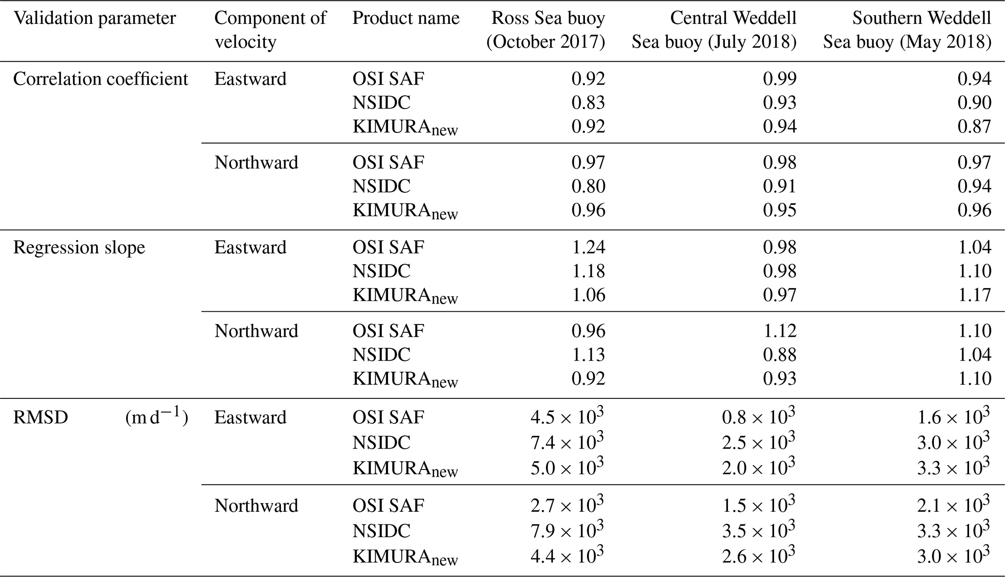
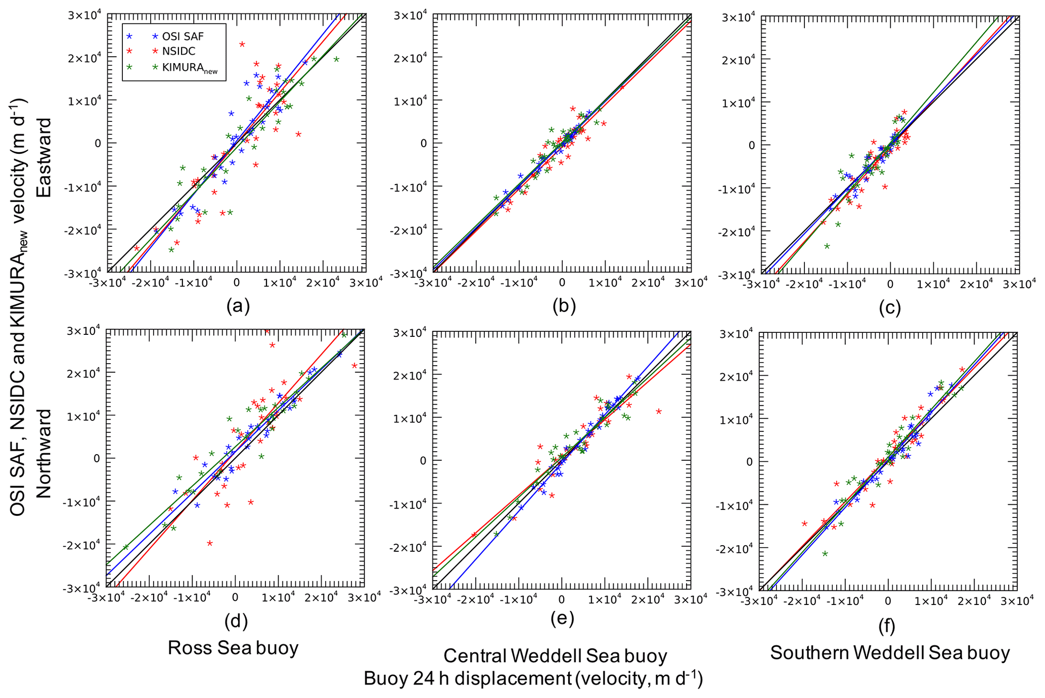
Figure A1 Scatterplot comparison of OSI SAF (blue), NSIDC (red), and KIMURA_new combined (green) products against buoy velocities (24 h displacement) in eastward (a, b, and c) and northward (d, e, and f) directions in October 2017 for the Ross Sea buoy, July 2018 for central Weddell Sea buoy, and May 2018 for southern Weddell Sea buoy. The solid black line represents a perfect regression slope of 1.0 with no offset.