the Creative Commons Attribution 4.0 License.
the Creative Commons Attribution 4.0 License.
 | 08 Apr 2022
Thermal structure of the Amery Ice Shelf from borehole observations and simulations
Chen Zhao
Rupert Gladstone
Ben Galton-Fenzi
Roland Warner
The Amery Ice Shelf (AIS), East Antarctica, has a layered structure, due to the presence of both meteoric and marine ice. In this study, the thermal structure of the AIS and its spatial pattern are evaluated and analysed through borehole observations and numerical simulations with Elmer/Ice, a full-Stokes ice sheet/shelf model. In the area with marine ice, a near-isothermal basal layer up to 120 m thick is observed, which closely conforms to the pressure-dependent freezing temperature of seawater. In the area experiencing basal melting, large temperature gradients, up to −0.36 ∘C m−1, are observed at the base. Three-dimensional (3-D) steady-state temperature simulations with four different basal mass balance (BMB) datasets for the AIS reveal a high sensitivity of ice shelf thermal structure to the distribution of BMB. We also construct a one-dimensional (1-D) transient temperature column model to simulate the process of an ice column moving along a flowline with corresponding boundary conditions, which achieves slightly better agreement with borehole observations than the 3-D simulations. Our simulations reveal internal cold ice advected from higher elevations by the AIS's main inlet glaciers, warming downstream along the ice flow, and we suggest the thermal structures dominated by these cold cores may commonly exist among Antarctic ice shelves. For the marine ice, the porous structure of its lower layer and interactions with ocean below determine the local thermal regime and give rise to the near-isothermal phenomenon. The limitations in our simulations identify the need for ice shelf–ocean coupled models with improved thermodynamics and more comprehensive boundary conditions. Given the temperature dependence of ice rheology, the depth-averaged ice stiffness factor derived from the most realistic simulated temperature field is presented to quantify the influence of the temperature distribution on ice shelf dynamics. The full 3-D temperature field provides a useful input to future modelling studies.
- Article
(14465 KB) - Full-text XML
- BibTeX
- EndNote


The Amery Ice Shelf (AIS) (Fig. 1; ∼ 70∘ S, 70∘ E) is the largest ice shelf in East Antarctica. It has an estimated floating ice area of 60 000 km2 (Galton-Fenzi et al., 2008), extending more than 550 km from its southern grounding zone to the ice front in Prydz Bay. The thickest region of the ice shelf is at the southern grounding zone, with a thickness of ∼ 2500 m (Fricker, 2002). The AIS is fed primarily by the Lambert, Mellor and Fisher glaciers, which account for 60.5 % of the total ice mass flux (Yu et al., 2010). The remaining ice flux across the grounding line is contributed by other tributaries on the eastern and western sides of the AIS. The AIS together with its inlet glaciers and their catchments is referred to as the Lambert-Amery Glacial System (LAGS).
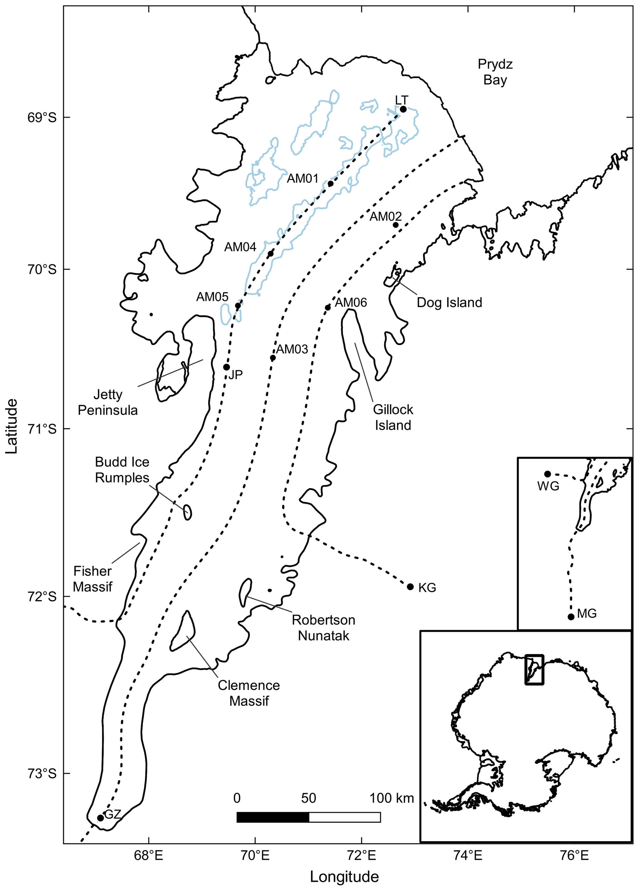
Figure 1The Amery Ice Shelf with significant features and AM01–AM06 borehole locations. Three dashed lines, derived from MEaSUREs InSAR-based Antarctic ice velocity data (Rignot et al., 2017), indicate the particular ice flowlines used in this study. The Jetty Peninsula flowline (hereafter JP flowline) starts from what we term the West Tributary Glacier (WG), passes through Jetty Peninsula point (JP), AM05, AM04 and AM01 boreholes, and ends at the “Loose Tooth” point (LT). The terminology of the flowline points JP and LT follows Craven et al. (2009), but the specific locations are slightly different. The AM03 flowline originates from Mellor Glacier (MG), passes through Grounding Zone point (GZ) and AM03 borehole, ending at the ice front. The AM06 flowline originates from Kronshtadtskiy Glacier (KG), passes through AM06 borehole and passes close to AM02 borehole. Marine ice regions with thickness greater than 100 m are shown with the light blue contours (Fricker et al., 2001). The locations of the grounding mask and the ice front are from Depoorter et al. (2013). Insets show the origins of the JP and AM03 flowlines and location of the AIS in East Antarctica.
The marine ice (i.e. basal ice formed from ocean water) layer under the AIS is an important feature of its overall structure, which could stabilise the ice shelf (Khazendar et al., 2009; Kulessa et al., 2014). Based on satellite radar altimeter and airborne radio-echo sounding (RES) measurements, Fricker et al. (2001) derived the spatial distribution of the marine ice layer under the AIS. The thickness of basal marine ice was estimated to be as great as 190 m (Fricker et al., 2001), while borehole measurements revealed that the thickness exceeds 200 m (Craven et al., 2004, 2005, 2009). Most of the marine ice is located in two longitudinal zones in the north-western AIS and extends along ice flowlines all the way to the ice front (light blue contours in Fig. 1; after Fricker et al., 2001).
The overturning ocean circulation under the ice shelf, together with changes in the in situ freezing point of seawater, contributes to the refreezing process and formation of marine ice (Lewis and Perkin, 1986). Observations obtained from borehole video cameras and instrument moorings (Craven et al., 2005, 2014) provided insights into the formation processes of the marine ice layer under the AIS and its structure. Frazil ice accretes and platelets consolidate at the ice–ocean interface, forming the original basal marine ice (Lambrecht et al., 2007; Craven et al., 2014; Herraiz-Borreguero et al., 2013; Galton-Fenzi et al., 2012). The newly formed marine ice, which is highly porous and hydrologically connected to the ocean below, slowly consolidates and undergoes a pore closure process (Craven et al., 2009). During the hot-water drilling at AM01 and AM04, a sudden change of the water level in the borehole indicated that drilling had established a hydraulic connection between the water-filled borehole and the ocean beneath the ice shelf, well above the actual ice shelf base (Craven et al., 2004, 2009). The remaining porous ice was still mechanically strong and had to be removed by continued drilling. The hydraulic connection depths are regarded as the interface between upper impermeable and lower permeable marine ice layers (Craven et al., 2009). Craven et al. (2009) also indicated that the cavities between the platelets account for more than 50 % of the total volume in the deepest marine ice, while the porosity of the impermeable marine ice is much lower. Due to the porous structure of the deeper marine ice layer, together with the presence of meteoric ice (i.e. ice formed from compacting snow) flowing from the continent and also deposited on the ice shelf, and the surface firn layer (Treverrow et al., 2010), the AIS has a layered vertical structure, which will be explored in this study by investigating its englacial temperature distribution.
Knowledge of the thermal structure of ice shelves is of high practical interest, and the internal temperature regime records the past climate and thermal conditions upstream (Humbert, 2010). Many studies have been carried out on the thermal structure of the ice sheets/glaciers (e.g. Jania et al., 1996; Ryser, 2014; Saito and Abe-Ouchi, 2004; Seroussi et al., 2013) and ice shelves (e.g. Budd et al., 1982; Craven et al., 2009; Humbert, 2010; Kobs et al., 2014). To explore the vertical temperature regime of ice shelves, hot-water drilling is commonly used to access the ice shelf interior (e.g. Craven et al., 2004; Makinson, 1994). Thermistor strings with surface loggers can provide long-term point borehole temperatures at different depths. In a modelling study, Humbert (2010) evaluated the thermal regime of the Fimbulisen (Fimbul ice shelf) based on thermistor data from a single borehole, which showed a cold middle part inside the ice shelf. However, these point sensors are not able to provide spatially continuous temperature measurements and the vertical resolution is limited by the number of thermistors. The fibre-optical temperature sensing, also known as distributed temperature sensing (DTS), is a better approach to achieve continuous in situ temperature measurements inside an ice shelf (e.g. Tyler et al., 2013). Among Antarctic ice shelves, DTS deployments were first made in the AM05 and AM06 boreholes of the AIS in 2009 (Warner et al., 2012). Kobs et al. (2014) derived the temperature gradient at the ice–ocean interface of the McMurdo Ice Shelf from high-resolution DTS data and also estimated seasonal basal melting using the evolution of the temperature gradient.
In the early stage of studies on the thermal regime of ice shelves, Wexler (1960) and Crary (1961) quantified the observed temperature profiles at sites on the Ross Ice Shelf and derived steady-state solutions for the profiles, which are functionally dependent on the basal melt rate. The earliest vertical temperature profile for the AIS was determined by measurements in the upper 320 m of the borehole G1 (69.44∘ S, 71.42∘ E; Budd et al., 1982), the same geographic location as the later AM01 site (Fig. 1). By fitting the measured temperature profile with the 1-D advection–diffusion equation, small temperature gradients were found within ∼ 100 m of the upper and lower surfaces, and the transition temperature gradient in between is uniform and relatively larger (Budd et al., 1982). The temperature profiles obtained later within the marine ice band at AM01 and AM04 borehole sites (Craven et al., 2009) also showed similar profile patterns. Craven et al. (2009) attributed the near-isothermal phenomenon of the bottom permeable layer to the accretion of marine ice as deposition of frazil ice platelets and suggested there is no conductive heat flux into the ice shelf from the ocean cavity.
The basal mass balance (BMB) of an ice shelf is the flux of basal melting or freezing (marine ice accretion; Galton-Fenzi et al., 2012). It is expected to have a significant influence on the vertical thermal structure (Kobs et al., 2014; Craven et al., 2009; Humbert, 2010). In this study, we explore the sensitivity of the thermal structure of the AIS to different BMB fields. A full-Stokes ice sheet model, Elmer/Ice (Gagliardini et al., 2013), is used to simulate three-dimensional (3-D) ice shelf dynamics and generate steady-state temperature fields using four different BMB fields for the AIS. We compare the simulated 3-D temperature fields with the observations at six borehole sites (AM01–AM06) to evaluate our simulation results and to find the most realistic temperature field. As a complement to the 3-D model, one-dimensional (1-D) temperature column simulations are designed to reconstruct the progress of ice columns moving along the flowlines with boundary conditions varying to correspond with position along the flowlines. We present the measured borehole temperatures in Sect. 2.1. The 3-D steady-state temperature simulations and 1-D temperature column simulations are introduced in Sect. 2.2 and 2.3, respectively. We present the corresponding results in Sect. 3 and discuss them in Sect. 4 before giving the conclusions in Sect. 5.
2.1 Borehole temperature measurements
The Amery Ice Shelf Ocean Research (AMISOR) project was launched to investigate ice–ocean interaction processes, the interaction with the interior grounded ice sheet and the properties of oceanic water masses beneath the ice shelf (Allison, 2003). As a part of the AMISOR project, from 2001 onwards, six boreholes, named AM01–AM06 (Fig. 1), were hot-water-drilled on the AIS (Craven et al., 2014). Sites AM01, AM04 and AM05 are located on approximately the same ice flowline where basal marine ice is present, and we name it the Jetty Peninsula flowline (hereafter JP flowline for simplicity) in this study. It originates from what we term the West Tributary Glacier (WG) of the AIS (Fig. 1). Sites AM02, AM03 and AM06 are in areas without basal marine ice where we determine another two specific flowlines (Fig. 1). The AM03 flowline originates from Mellor Glacier (MG), passing through the AM03 borehole. The AM06 flowline, from Kronshtadtskiy Glacier (KG), passes through the AM06 borehole and passes close by the AM02 borehole.
After hot-water drilling, the boreholes were kept open for several days to make observations in the ocean cavity, and deploy oceanographic mooring instruments (Craven et al., 2004) and thermistor strings (or optical fibres) for long-term measurements. Two thermistor strings were deployed within and through each of the earlier boreholes, AM01–AM04. One was used to measure the internal ice shelf temperature, and the other was for tracking the ice–ocean interface. All the internal thermistor data points are used in this study, while only a few characteristic thermistor data points at the ice–ocean interface are selected, since the interface thermistors are closely distributed along the cable, and the differences between readings for those thermistors are insignificant. The Sensornet Oryx instruments (distributed temperature sensors) and optical fibres were deployed at AM05 and AM06 sites, which provided continuous profiles of the temperature distribution along the fibre cable with a spatial sampling interval of 1.015 m. Temperatures within the top 10 m of the firn layer were recorded by automatic weather stations (AWSs) of the Australian Antarctic Programme at AM01 and AM02 boreholes and at the Amery G3 site (70.891∘ S, 69.871∘ E), which is approximately 42 km south of AM03, and these showed clear seasonal signals. Similar signals were also observed within the top 10 m of the firn layer on the McMurdo Ice Shelf (Kobs, 2014). To eliminate these near-surface seasonal signals and derive “steady-state” vertical temperature profiles at the borehole sites for comparison with the simulations, some temperature data near the top surface at AM01–AM04 have been carefully selected and temporally averaged. Temperatures at 10 m depth at AM01 and AM02 are temporally averaged from the collocated AWS records in the corresponding time interval (Table 1), while the near-surface temperatures at AM03 and AM04 are estimated with reference to all the available AWS data in the corresponding time interval and a multi-year average surface temperature field over 1979–1998 (Comiso, 2000). At AM05 and AM06, the DTS data within 20 m of surface are not considered, due to strong seasonal signals. Details about the temperature data, including the depths of the measuring instruments, are presented in Table 1. We note that the temperature profiles of AM01 and AM04 based on thermistor string data have been published in Craven et al. (2009) and Treverrow et al. (2010).
Table 1Details of the borehole thermistor data at sites AM01–AM04 and DTS data at sites AM05 and AM06 in the AIS. The DTS conducts continuous temperature measurements with a spatial sampling interval of 1.015 m. Temperatures at sampling depths marked in parentheses are estimated using the available regional AWS data and surface temperature field (Comiso, 2000) or in situ pressure melting temperature as appropriate; depths in bold are within the marine ice layer.
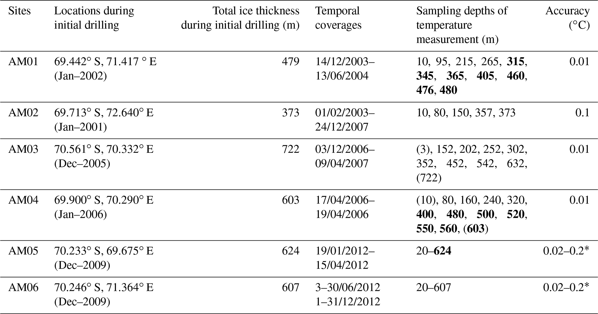
∗ Attainable DTS accuracy for the internal temperatures varies from 0.2 ∘C around −20 ∘C to 0.02 ∘C around −2 ∘C. This variation is due to the availability of accurate in situ calibration data.
After the temperature-measuring instruments are deployed, the water in the boreholes refreezes in a relatively short time, while the borehole temperatures take a much longer time to fall back to equilibrium. This cooling process can be detected within each borehole, assuring thermal disturbance produced by the drilling has basically dissipated and the borehole thermal regime is in approximate equilibrium. The internal thermistors at AM01 recorded a rapid drop of borehole temperatures during 15 d after instruments were deployed, and after 40 d they were still slowly decreasing at a rate of 0.04 ∘C d−1, illustrating the long-term adjustment to the original temperature regime before hot-water drilling. The temperature observations at AM01–AM04 sites lasted for several years until 2009. However, during this period, battery exhaustion and surface logger failures resulted in multiple measurement interruptions, and individual thermistor failures also led to the loss of data in space over the long-term measurement. Since January 2010, the distributed temperature sensors recorded borehole temperature along the optical fibres at AM05 and AM06 until 2013, but data gaps in these time series also exist due to operational difficulties. The non-equilibrium data disturbed by drilling work and the data with errors due to equipment failures are eliminated in this study. The temporal coverages of near-equilibrium temperature data used are listed in Table 1. A frozen-in device, either a thermistor string or a distributed temperature sensor, is a “Lagrangian” measuring instrument, advected horizontally and vertically by the flow of the ice shelf. The locations of the six boreholes during the initial drilling process are used for subsequent analysis in this study, presented in Table 1.
2.2 The 3-D steady-state temperature simulations
For our 3-D modelling study, we carry out a series of simulations for the entire Lambert-Amery Glacial System (LAGS), which involves modifying the dynamic boundary condition at the base of the ice shelf to impose four different BMB fields. The main aim of our 3-D simulations is to explore the sensitivity of the thermal structure of the AIS to different BMB fields. We then compare the simulated 3-D temperature distributions of the AIS with the borehole observations to evaluate our simulation results. The simulations presented here build on a larger study concerning optimisations in a regional Antarctic ice sheet model (methodology described by Gladstone and Wang, 2022), and we take simulations from that work for our starting point, as detailed in the next section. All the simulations are implemented using the Elmer/Ice model (Gagliardini et al., 2013), a finite-element, full-Stokes ice sheet/shelf model, which also has the capacity to calculate the englacial temperature distribution.
From that starting point (Gladstone and Wang, 2022), we first optimise the ice flow dynamics across the LAGS for each choice of ice shelf BMB forcing. We do this by optimising spatial distributions of basal resistance and ice viscosity using adjoint inverse methods (Gillet-Chaulet et al., 2012), with the observed horizontal surface velocities (Rignot et al., 2017) as our optimisation target. After these diagnostic simulations of the dynamics, we perform simulations for the 3-D steady-state temperature distribution using the newly optimised ice dynamics (the strain rates and 3-D velocity fields). The complete simulation workflow is shown in Fig. 2, where each simulation uses the optimised parameters from the previous stage.
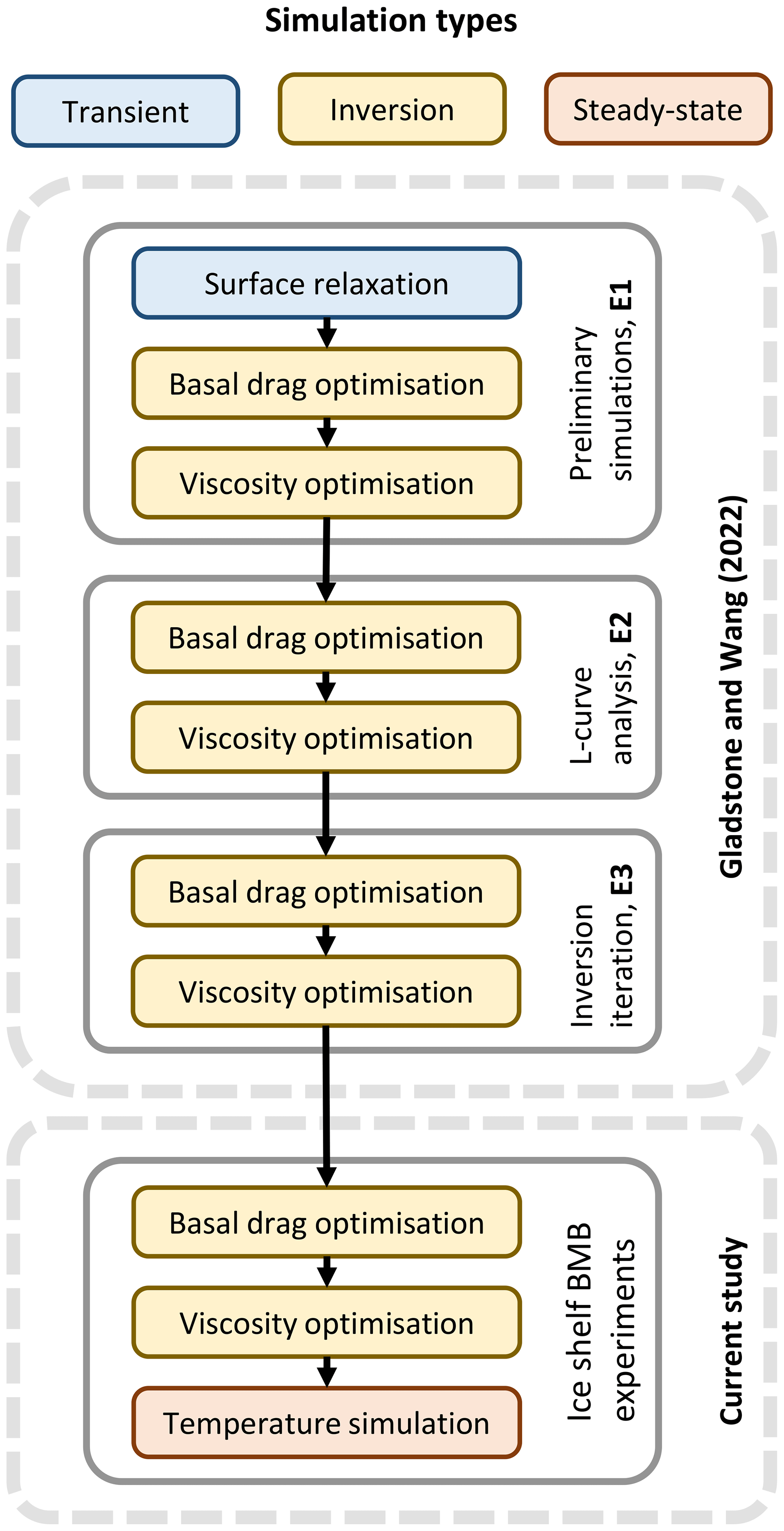
Figure 2Overview of the 3-D simulation workflow in this study. Simulations are indicated in coloured boxes. Experiments are indicated in grey outlined boxes. Arrows indicate the use of the final model state from a simulation to initialise the following simulation. Experiment E1, E2 and E3 are from Gladstone and Wang (2022), while the ice shelf BMB experiments are carried out in the current study.
2.2.1 Modelling background and initial state for the simulations
As detailed by Gladstone and Wang (2022), a sequence of ice flow dynamics simulations was performed, consisting of three experiments (Fig. 2), namely, a preliminary simulation (E1), L-curve analysis (E2) and inversion iterations (E3). These three experiments include a short initial prognostic simulation to permit surface relaxation, and a series of diagnostic simulations of ice dynamics. The diagnostic simulations use the adjoint inverse method (Gillet-Chaulet et al., 2012) to optimise both basal resistance and ice viscosity and also take the observed horizontal surface velocities (Rignot et al., 2017) as the optimisation target. The dynamic boundary conditions for these experiments E1–E3 are the conventional ones: a stress-free upper surface, basal conditions of tangential frictional stress and vanishing normal velocity for the grounded ice, and vanishing tangential stresses and normal stress balancing ocean pressure for the ice shelf. These simulations all use a 3-D internal ice temperature distribution generated by a multi-millennial spin-up with the SICOPOLIS model (Greve et al., 2020; Seroussi et al., 2020). Ice geometry is from BedMachine Antarctica (Morlighem, 2019; Morlighem et al., 2020). The 3-D mesh of the LAGS domain has 20 layers vertically for a total of approximately 1 million bulk elements. The elements range in size from approximately 2 to 15 km in the horizontal, with finer resolution where gradients in ice thickness and velocity are greater. The detailed simulations, inversion process and settings (including mesh generation and boundary conditions) are described in full by Gladstone and Wang (2022). The current study uses the final model state of their experiment E3 as our starting point (Fig. 2), including the optimised basal resistance parameter β and viscosity enhancement factor Eη. The spatial distributions of the two parameters are shown in Fig. 3a, b respectively. More specifically, the optimised dimensionless basal resistance parameter β (Fig. 3a) governs the basal sliding through the relation:
where τb is basal resistance, ub is sliding speed and Cb is a basal resistance coefficient of 1 MPa m−1 a. The optimised viscosity enhancement factor Eη (Fig. 2b) varies the viscosity η of the deforming ice from that derived from Glen's flow law (Glen, 1958; Paterson, 1994):
where n is the exponent in Glen's flow law; A(T′) is the corresponding deformation rate factor, dependent on T′, the ice temperature relative to the pressure melting point; and is the effective strain rate. Values of Eη greater than 1 indicate stiffer ice than predicted by Glen's law, while values between zero and 1 indicate softer ice.
Figure 3c shows the relative difference in surface horizontal velocities between simulations from the final model state of experiment E3 and observations (Rignot et al., 2017). The relative velocity difference in the ice shelf is mostly less than 10 %, while the difference in the fast-flow area (where surface velocity > 300 m a−1) is mostly less than 2 %. This suggests that the experiment E3 from Gladstone and Wang (2022) provides a reliable starting point for the experiments in this paper.
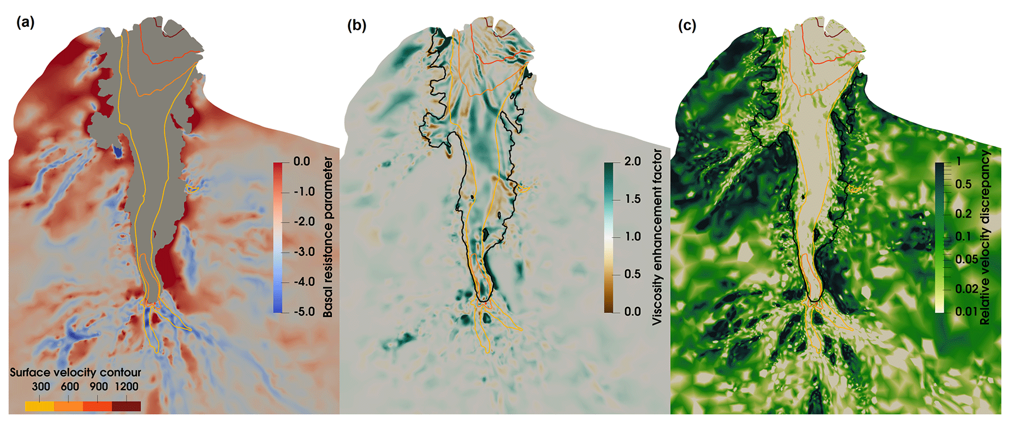
Figure 3The optimised basal resistance parameter β (a), viscosity enhancement factor Eη (b) and relative surface horizontal velocity discrepancy (c) for the LAGS in the final state of experiment E3 of Gladstone and Wang (2022). The relative surface velocity discrepancy is the magnitude of the surface horizontal velocity difference between observations (Rignot et al., 2017) and simulations as a fraction of the observations. The four contours represent the surface velocity of 300, 600, 900 and 1200 m a−1 respectively, extracted from the final state of experiment E3. The black line in (b) and (c) represents the grounding line from BedMachine Antarctica (Morlighem, 2019; Morlighem et al., 2020).
2.2.2 Ice shelf basal mass balance experiments
From the final model state of experiment E3, we first carry out diagnostic simulations for the basal resistance and ice viscosity inversions across the whole LAGS (Fig. 2). We essentially follow the inversion procedures of the experiment E3 in Gladstone and Wang (2022), taking the observed surface velocities (Rignot et al., 2017) as the optimisation target and using a 3-D ice temperature field from the SICOPOLIS modelling (Greve et al., 2020; Seroussi et al., 2020) throughout the two inversion steps (Fig. 2). Tikhonov regularisation parameters (Gillet-Chaulet et al., 2012; Morlighem et al., 2010) of 103 and 104 are used for basal resistance and viscosity inversions respectively, following the L-curve analysis by Gladstone and Wang (2022).

Figure 4The basal mass balance distributions: (a) BMB_ISMIP6, (b) BMB_ROMS, (c) BMB_CAL and (d) BMB_CAL2. Negative implies basal melting, and positive implies freezing. White dots are the locations of AM01–AM06 boreholes, as shown in Fig. 1. Non-linear colour scales are used to cover the large melting rates. Areas with a melting rate greater than 15 m a−1 are represented by purple, with maximum melting rates exceeding 40 m a−1 for some distributions.
The four BMB datasets for the AIS used in the experiment are shown in Fig. 4. The first BMB dataset, BMB_ISMIP6, uses the Ice Sheet Model Intercomparison Project (ISMIP6) “local quadratic melting parameterisation” (Jourdain et al., 2020; Seroussi et al., 2020). This is the only BMB dataset we use that does not feature refreezing. The second BMB dataset, BMB_ROMS, is derived from modelling of the basal ice–ocean thermodynamics and frazil dynamics by Galton-Fenzi et al. (2012), using the Regional Ocean Modelling System (ROMS). The third, BMB_CAL, is from Adusumilli et al. (2020), derived from satellite remote sensing data using an ice flux divergence calculation (assuming ice shelves are in steady state). To explore the response of the simulated temperature field to a higher basal accretion rate in our fourth mass balance dataset, BMB_CAL2, we double the basal freezing rate of BMB_CAL while keeping the melt rate the same (i.e. positive mass balance values are doubled, while negative values are left unchanged).
To explore the influence of the various proposed BMB fields, we directly impose the BMB as a Dirichlet condition on the component of ice velocity in the direction normal to the lower surface of the shelf, replacing the conventional basal boundary condition of matching the normal stress to the ocean pressure. Specifically, basal melting and freezing correspond to an outward (approximately downward) and inward (approximately upward) velocity, respectively, at the lower boundary. This implicitly assumes that the ice shelf base is in steady state. For the grounded area, the basal dynamic boundary conditions remain unchanged: the normal component of ice velocity vanishes at the bed.
For the upper surface dynamic boundary condition, instead of the conventional scheme of a completely stress-free upper surface, we adopt a resistive stress τr in the direction normal to the upper surface, the necessity and advantages of which we detail in Appendix A. The resistive stress τr we use is given as
where u is the modelled velocity, ns is the outward unit normal vector at the ice surface, Cs is a surface resistance coefficient, u∗ is a reference speed and ∥uobs∥ is the magnitude of the horizontal upper surface velocity from observations. We use a surface resistance coefficient Cs=50 MPa m−1 a and a reference speed m a−1. This is one of the parameterisation schemes for the upper surface dynamic boundary condition in experiment E5 described in Gladstone and Wang (2022). At the upper surface of the model, the emergence velocity (the component of the velocity in the outward normal direction, u⋅ns) should reflect the surface mass balance (SMB), if the ice geometry and flow are in steady state.
The optimised β and Eη obtained from the two inversion stages produce different 3-D velocity fields for each of the four BMB datasets. We then generate the corresponding 3-D steady-state temperature distributions using these velocities. This is done by solving the steady-state advection–diffusion equation, incorporating the appropriate internal strain heating and the frictional heating at the bed. As boundary conditions for the temperature solution, the upper surface temperature is fixed by the mean surface air temperature field over 1979–1998 described in Comiso (2000). The temperature at the lower surface of the ice shelf is specified as the pressure-dependent freezing temperature of seawater (using the ice shelf draft and a salinity of 35 psu) as a Dirichlet condition. The spatial distribution of geothermal heat flux (Martos et al., 2017), as estimated from airborne magnetic data, is used under the grounded ice of the LAGS, as a Neumann condition.
2.3 The 1-D temperature column simulations
To explore the formation of the vertical thermal structure in the areas with and without basal marine ice, we also conduct 1-D column simulations based on time-stepping to follow columns of ice along the JP flowline and AM03 flowline (Fig. 1), respectively. A pioneering application of this approach was made by Macayeal and Thomas (1979) to interpret the formation of the measured temperature profile at J9 borehole on the Ross Ice Shelf. In the current study, a model of a vertical ice column with 100 equally spaced layers is constructed using Elmer/Ice. A series of key sites along the two flowlines, as shown in Fig. 1, are determined as key time stamps. The time intervals between each time stamp are derived according to the spatial locations of the key sites and the surface velocity field of the AIS (Rignot et al., 2017). Figure 5, as a schematic diagram, demonstrates the evolution of an ice column along each flowline, with related column parameters and boundary conditions as shown. Each 1-D experiment consists of a series of simulations using temperature solvers in Elmer/Ice and involves two stages: initial spin-up and forward transient simulations.
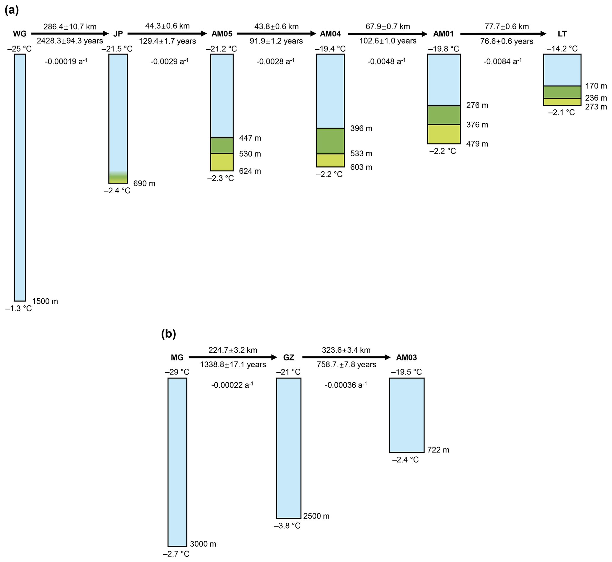
Figure 5Schematic diagrams of the 1-D temperature column simulations along (a) the JP flowline and (b) the AM03 flowline. In (a), from the top: meteoric ice (blue), impermeable marine ice (dark green) and permeable marine ice (light green). At JP, there are no observations indicating the condition of marine ice. Between the key sites, length along the flowline, time interval and calculated vertical strain rate are marked respectively. The upper and lower surface temperature and ice layer thickness are also marked. Ice layer thicknesses at JP, AM04, AM01 and LT are from Craven et al. (2009); AM03 thickness is from measurements during drilling; AM05 layer thicknesses are estimated based on DTS data in this study (see Sect. 3.1); the thicknesses at WG, MG and GZ are extracted from BedMachine Antarctica (Morlighem, 2019; Morlighem et al., 2020). The increase in the width of the ice column qualitatively illustrates the strain thinning process along the flowlines.
The initial spin-up is a steady-state temperature simulation used to initialise the vertical thermal regime of a column of grounded ice at the start of each flowline (WG and MG; see Figs. 1 and 5). Starting from the initial steady state, we then perform forward transient simulations representing evolution of the ice column as it is advected through the ice sheet and ice shelf (Fig. 5). The transient simulations also implicitly involve a steady-state assumption, since our ice columns are assumed to move strictly along the ice streamline of the reference horizontal velocity field (Rignot et al., 2017), and the boundary conditions we use do not incorporate temporal records but represent the appropriate location along the streamline.
We impose boundary conditions, including the mass balances and temperatures at the upper and lower surfaces of the column model, advancing by 1-year time steps between the key time stamps. The surface temperature is determined at each key time stamp (Fig. 5), based on all available AWS observations and multi-year surface mean temperature dataset (the same as used in our 3-D simulations; Comiso, 2000), and is linearly interpolated between time stamps. Similarly, the basal temperature at each key time stamp is taken from borehole observations (where available) or as the calculated in situ pressure melting temperature (Fig. 5), also linearly interpolated between time stamps. According to the location of the ice column at each time step, the SMB is interpolated from the gridded 1979–2016 mean data of RACMO2.3p2 (a regional atmospheric model; Van Wessem et al., 2018). Similarly, the BMB within the floating sector is extracted from Adusumilli et al. (2020) (i.e. BMB_CAL), while zero BMB is imposed for the grounded ice. Ice thus flows vertically across the upper and lower surfaces of the column according to these imposed mass balance (melting/freezing rates) in the column simulations. The ice thickness of the column model at each key site (time stamp) is also fixed, based on borehole measurements and BedMachine Antarctica (Morlighem, 2019; Morlighem et al., 2020), while the vertical strain rates for each interval between key sites (always strain thinning; marked in Fig. 5) are selected to adjust the column thickness variations, in conjunction with imposed mass balance, to fit the prescribed ice thicknesses at the key sites. The vertical velocity in the ice column, taken as varying linearly with depth, is thus determined by the prescribed SMB, BMB and vertical strain rate.
In general, the initial setup of the spin-up and the boundary conditions for the transient simulations are inferred from a variety of available data. In addition to the steady-state assumption, there are a series of other assumptions:
-
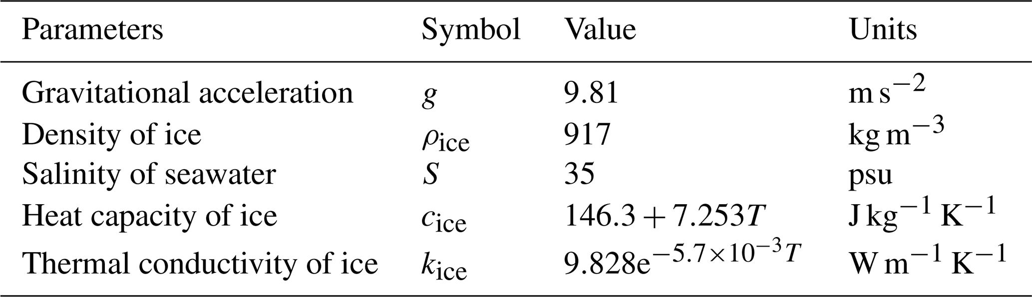
The ice density of the column is taken as constant everywhere and will not change with the vertical strain process. The heat capacity and conductivity are functions of in situ ice temperature. The ice accreted at either surface in the simulations is assumed to have the same material properties. Detailed physical parameters are shown in Table 2.
-
There is no horizontal shear in the ice column. The horizontal ice flow in our 1-D experiment is simply considered to be a plug flow. The ice column stays vertical all the time, and its height changes only by imposed accretion/melting on both surfaces and vertical strain.
-
There is no thermal conduction in transverse direction, (i.e. no heat flux through the lateral boundaries of the column) since the horizontal temperature gradient is considered to be much smaller than that in the vertical direction.
-
The basal temperature of grounded ice, as a Dirichlet condition, is assumed to be always at the pressure melting point of ice.
The column temperature profile can be extracted from the transient simulations at any temporal point, which corresponds to a certain spatial point on the flowline. Therefore, the simulations can be evaluated by comparing the simulated column temperature profile at the borehole sites with borehole measurements.
Table 2Standard physical parameters of the 1-D temperature column simulation. The heat capacity, cice, and thermal conductivity, kice, are functions of temperature, T, in K (Ritz, 1987).
3.1 Borehole thermal regimes
The measured temperature profiles within the boreholes are relatively stable over the selected observation periods. The thermistors in AM01 and AM03 boreholes show a slight decrease in temperature within 0.05 ∘C during the temporal coverages (Table 1), which we attribute to continuing adjustment towards the original ice temperatures after hot-water drilling. The DTS time series in AM05 and AM06 suggest random fluctuations (noise) of ±0.05 ∘C in individual observations at any given depth, which are reduced to ±0.01 ∘C by averaging consecutive measurements. This may be regarded as indicating the precision that the DTS can provide. However, the averaging process also reveals small systematic differences between adjacent depths, which points to limits on accuracy, although usually accuracy is limited by availability of precision calibration data. Borehole thermal regimes are derived from averaging all those measurements (Table 1) selected to represent the thermal equilibrium state. To achieve continuous temperature profiles, spline interpolation is used to smoothly connect the discrete thermistor points to compare with DTS profiles. Figure 6 shows the borehole temperature profiles at AM01–AM06 grouped as with or without basal marine ice, where the profiles of AM02, AM03, AM05 and AM06 boreholes are published here for the first time. Our time-averaged temperature profiles of AM01 and AM04 boreholes are consistent with the previously published temperature profiles (Craven et al., 2009; Treverrow et al., 2010).
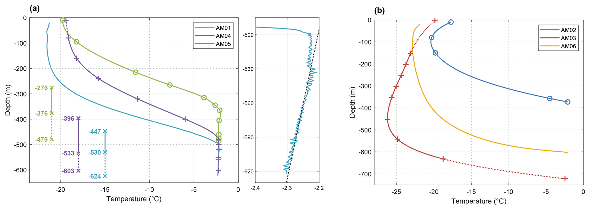
Figure 6Borehole temperature profiles (a) at AM01, AM04 and AM05 (with marine ice) and (b) at AM02, AM03 and AM06 (without marine ice). The subplot of (a) is the near-isothermal section of AM05, fitted with an in situ seawater freezing line for a salinity of 34.4 psu. Markers (+) and (o) indicate the thermistor points. The depth ranges (lower left of a) mark impermeable (solid line) and permeable (dotted line) marine ice layers from Fig. 5a. The temperatures of the upper and lower surfaces at AM03 and AM04 are inferred from available AWS data and the surface air temperature field (Comiso, 2000), represented by dotted lines.
AM01, AM04 and AM05, approximately located on the same flowline in the marine ice band (the JP flowline; Fig. 1), show similar profile patterns (Fig. 6a). The temperature profiles at these sites show nearly isothermal basal layers up to 120 m thick, which are closely related to the in situ pressure-dependent freezing point of seawater. The correlation is well reflected in the DTS profile at AM05 (subplot of Fig. 6a), where the profile for 530–624 m depth is well approximated by a constant salinity in situ pressure freezing line. The observed pressure-dependent temperature suggests that the marine ice below 530 m depth maintains a hydraulic connection with the ocean below. There is a slight step at 530 m depth. Fresher water from the drilling process was observed above this level prior to borehole freeze-up. The profile above 530 m depth no longer matches the pressure freezing line, implying the termination of the hydraulic connection, and at 500 m there is an abrupt change in the temperature gradient. Therefore, we estimate that at AM05, the interface between permeable and impermeable marine ice (corresponding to the hydraulic connection depths observed at AM01 and AM04 by Craven et al., 2009) is around 530 m depth (marked in Fig. 6a). The temperature at the interface between meteoric and impermeable marine ice drops from 6.2 ∘C at AM04 to .8 ∘C at AM01 over the period of 102.6 years. If it is assumed that the interface temperature drops at the same rate from AM05 to AM04, the temperature of the meteoric–marine ice interface at AM05 can be estimated to be −5.8 ∘C. Combined with the observed temperature profile of AM05, the interface depth can then be estimated as 447 m (marked in Fig. 6a), corresponding to a marine ice thickness of 177 m at AM05. This estimation is in good agreement with the marine ice thickness expected on the basis of vertical strain thinning and basal accretion from AM05 to AM04. The internal temperature gradually increases along the JP flowline, while the internal temperature gradients remain stable and relatively high (Table 3) above the isothermal zone at these three sites. At AM05, the upper 200 m of the meteoric ice is nearly isothermal, and the corresponding layer is thinned to ∼ 100 m at AM04, then approximately dissipated at AM01.
Table 3Observed temperature gradients and derived corresponding heat fluxes at the base of the meteoric ice at the six borehole sites. The heat flux is calculated according to Fourier's law, including the fact that thermal conductivity of ice, kice, is a function of ice temperature as shown in Table 2.
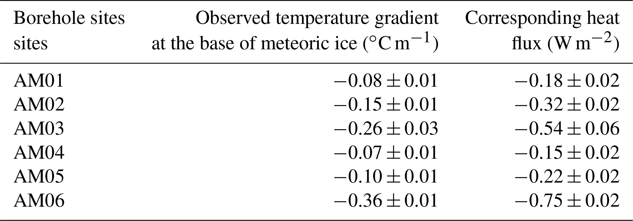
AM02, AM03 and AM06, in the area without marine ice, show large temperature gradients within 100 m of the lower surface layer (Fig. 6b). AM02 and AM03 reveal significantly colder ice in the interior of the ice shelf column than at the upper surface, hereafter referred to as “cold cores” in the ice shelf. The temperature gradients at the base of the meteoric ice, as well as the corresponding heat flux, derived from the borehole temperature profiles are shown in Table 3. At sites AM02, AM03 and AM06 without a marine ice layer, the heat flux represents that across the ice shelf–ocean interface.
3.2 Results from 3-D steady-state temperature simulations
The basal resistance and viscosity inversions performed in each of our ice shelf BMB experiments produced very similar distribution patterns to those of experiment E3 (Gladstone and Wang, 2022) shown in Fig. 3a and b. The level of agreement of the modelled surface velocities with observations is consistent with the result of E3 (Fig. 3c). The quality of the fits to surface velocities achieved across the four BMB experiments shows very little variation. For example, in the BMB_CAL experiment, the magnitude of surface velocity mismatch between simulations and observations (Rignot et al., 2017) for 90 % of the surface nodes on the ice shelf is less than 20 m a−1, and the average magnitude of the velocity mismatch is 8.8 m a−1. This suggests that the dynamic basis of the temperature simulation results is reliable.
A set of 3-D steady-state temperature distributions are computed using the results of the dynamical simulations with the four different BMB datasets described in Sect. 2.2. The simulated temperature profiles at the six borehole sites are extracted from these 3-D temperature fields (Fig. 8). Normalised depth, (where D is the depth below the upper surface and H is the ice thickness), is used to facilitate comparisons between the simulated and measured vertical temperature profiles. This is more convenient due to thickness differences between borehole measurements and the BedMachine data (Morlighem, 2019; Morlighem et al., 2020) used in the model (Fig. 7). Within the marine ice band, the total ice thickness at sites AM01, AM04 and AM05 in the model is ∼ 60 m less than the borehole measurements, while the differences at sites AM02, AM03 and AM06 are significantly smaller, no more than 20 m.
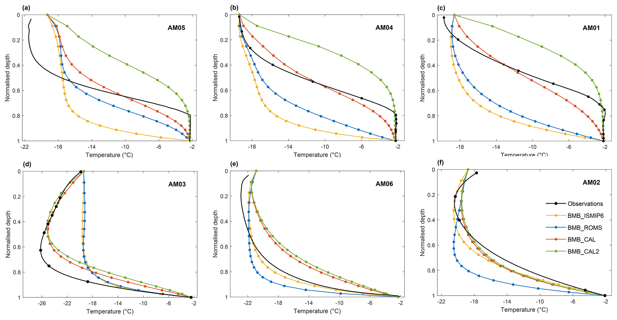
Figure 7Normalised-depth comparisons between measured and simulated temperature profiles at six borehole sites, shown in Fig. 1. AM05, AM04 and AM01 (a, b, c) are on the JP flowline from upstream to downstream with marine ice. AM03, AM06 and AM02 (d, e, f) are from upstream to downstream, experiencing basal melting. Observed temperature profiles are derived from the borehole thermistor (AM01–AM04) and DTS data (AM05, AM06). The 3-D model has 20 layers in the vertical, with circles indicating nodes.
The extracted simulated temperature profiles for the different BMB choices show different shapes at the six sites (Fig. 7), which reflect significant differences between simulated temperature fields. Differences between the various simulations and the borehole measurements at the upper surface are found at each site, especially for AM05, because the upper surface temperature in the simulations is fixed by the Antarctic surface temperature dataset (Comiso, 2000). As shown in Fig. 7, the simulation with BMB_ISMIP6 provides reasonable fitting at AM02 and AM06 (within the basal-melt area) but poor fitting at the sites with basal marine ice (AM01, AM04 and AM05) compared with other experiments, which is expected since BMB_ISMIP6 purely represents basal melting in those marine ice regions (Fig. 3a). The simulation with BMB_ROMS fits the borehole temperature profiles slightly better at the sites with marine ice, since basal accretion is considered in BMB_ROMS, while at AM02 and AM06 the effect of higher melt rates (see Fig. 3b) leads to poorer agreement than for BMB_ISMIP6. The BMB_ISMP6 and BMB_ROMS simulations give very similar but poor matches at AM03. The simulation with BMB_CAL provides better fitting results at most of the borehole sites but still does not reconstruct the near-isothermal marine ice layer at the bottom. In contrast, the simulation with BMB_CAL2 shows a much closer agreement in the lower part of the marine ice layer, which is visually close to the pressure freezing temperature line in the permeable marine ice layer. However, the manually increased basal accretion in BMB_CAL2 also leads to a severe overestimation of temperatures for the colder ice above the near-isothermal layer. For the sites outside the marine ice band (AM01, AM03 and AM06), the simulated temperature profiles from BMB_CAL and BMB_CAL2 show little difference. In general, the temperature field simulation with BMB_CAL best fits most of the borehole temperature profiles visually, which suggests that BMB_CAL is more representative of the real mass balance at the ice–ocean interface. Therefore, we mainly conduct detailed analysis and discussion on the simulations with BMB_CAL in the remainder of the paper.
To visualise the simulated steady-state temperature field, the depth-averaged temperature distribution and a series of temperature sections along and across the three flowlines are extracted from the simulation of BMB_CAL, as shown in Figs. 8 and 9. We note that the three flowlines here are derived from the simulated velocity field of the inversion simulations, which is almost the same as those obtained from the MEaSUREs Antarctica ice velocity data (Rignot et al., 2017). The distribution pattern of the depth-averaged temperature is strongly aligned with the ice shelf flow (Fig. 8). The depth-averaged ice temperature gradually increases downstream along the flow, which is the clearest along the AM03 flowline.

Figure 8Depth-averaged temperature distribution of the AIS from the 3-D simulations with BMB_CAL. Three flowlines, derived from simulated velocity field, and two crossing lines are marked with dashed lines. Marked letters (a–e) correspond to the sequence of cross-sections in Fig. 9. Marine ice band with estimated thickness greater than 100 m is shown with the light blue contours (Fricker et al., 2001). Inset shows the location of the Amery Ice Shelf in East Antarctica.

Figure 9Temperature sections from the 3-D temperature simulation with BMB_CAL, along (a–c) and across (d–e) the three flowlines shown in Fig. 8. The three flowlines are (a) JP flowline, (b) AM03 flowline and (c) AM06 flowline from west to east, derived from the simulated velocity field. In (a)–(c), the translucent black curve presents the basal mass balance (BMB_CAL) along the flowline. The positions of key points on the flowline are marked; all boreholes are shown with vertical dashed lines. In coordinates, “distance along flowline” is relative to the grounding line.
All the simulated temperature sections (Fig. 9) show internal cold ice advected from upstream inlet glaciers, originally formed due to downward advection of ice from cold, high-elevation regions far inland. The minimum internal temperature on the AM03 flowline is 28 ∘C, lower than that of the JP flowline (22 ∘C) and AM06 flowline (24 ∘C). The cold ice is gradually warmed along the flowlines by heat conduction from warmer ice both above and below, as it propagates toward the ice front. Along the three flowlines, the tens of kilometres near the grounding line reflect the transition of the thermal structure from grounded ice sheet to floating ice shelf, all of which experience the steepening of the basal temperature gradient, associated with active basal melting. Along the JP flowline (Fig. 9a), the internal cold core, warmer than that of the AM03 flowline, gradually warms up and dissipates around JP (Fig. 9a, d). Marine ice starts to accrete around 150 km downstream of the grounding line (see the BMB curve in Fig. 9a), where the basal temperature gradient starts to decrease. The vertical temperature regime in the marine ice zone downstream of AM05 maintains a consistent profile (Fig. 9a). The simulated (and observed) vertical temperature profiles at AM05, AM04, and AM01 are all similar (Fig. 7a, b, c), essentially just scaling as the ice shelf thins despite the continuing accretion of marine ice. Along the AM03 flowline (Fig. 9b), the ice thickness decreases rapidly within 100 km downstream of the grounding line, accompanied by a significant steepening of the temperature gradient of the lower part of the ice shelf, where it experiences considerable basal melting (see the BMB curve in Fig. 9b). The large basal temperature gradient gradually eases until 200 km downstream of the grounding line where a BMB close to zero is reached. The cold core, approximately 30 km wide at AM03 (Fig. 9d), is mainly composed of the cold continental ice from the Mellor and Lambert glaciers, flowing through the southern grounding line of the AIS. Along the AM06 flowline (Fig. 9c), the temperature section illustrates the formation of cold core ice within the ice shelf. Internal temperature of the ice shelf upstream of AM06 is close to the surface temperature (Fig. 9c, d). The surface temperature increases significantly downstream of AM06, at which time the internal temperature is lower in comparison, resulting in the formation of a cold core. It can be found at AM02 (Fig. 9c, e) and propagates downstream all the way to the ice front. The basal temperature gradient along the AM06 flowline is relatively small upstream of AM06, associated with a gentler basal melting than the other two flowlines.
The transverse temperature sections exhibit a great variation in the thermal structure across the ice flow (Fig. 9d, e). Based on the AM01–AM02 transverse temperature section (Fig. 9e), in addition to the cold core on the AM03 flowline and at AM02, there is also internal cold ice (at 50–70 km along the transverse section) that has entered from Scylla and Charybdis glaciers to the west. The basal warm ice layer at AM01 is ∼ 30 km wide (75–105 km along the same section), which correlates well with the pattern of the marine ice band (Fig. 8). Similarly, the basal warm layer to the west, ∼ 30 km wide (15–45 km along the section), also corresponds to the distribution of the western marine ice band (Fig. 8).
To quantify the influence of englacial temperatures on ice viscosity (Eq. 2) we introduce a temperature-dependent ice stiffness factor: . Motivated by Humbert (2010), we calculate the distribution of the depth-average of B(T′) across the AIS, , using the steady-state temperature field of the BMB_CAL simulation (details presented in Appendix B) to illustrate the spatial variation of this aspect of the ice shelf dynamics. The pattern (Fig. B1) is very similar to that of the depth-averaged temperature (Fig. 8). The depth-averaged ice stiffness factor achieves its maximum east of the AM03 flowline, approximately 70 km downstream of the grounding line, once the warmer lower layers of ice flowing in from the continent have been melted away (Fig. 9b). As the ice keeps progressively warming along the flowlines downstream (Figs. 8; 9a, b, c), the decreases, corresponding to softening of the ice, while there is also significant lateral variation in stiffness across the ice flow. In most areas of the AIS (86 % in area), is between 1×10⁸ and 1.8×10⁸ Pa s, with an average value of 1.48×10⁸ Pa s.
3.3 Results from the 1-D temperature column simulations
The use of the column model allows the specification of both the vertical velocity profile at each time step (or location) and, implicitly, the horizontal velocity along the flowline, in contrast to the 3-D modelling, where vertical velocities emerge from the 3-D dynamical simulations. A series of column simulations provides solutions for the time-stepping of the vertical 1-D advection–diffusion equation with specific boundary conditions (as discussed in Sect. 2.3). Vertical temperature profiles for each borehole on the two flowlines are extracted and compared with those from the 3-D simulation of BMB_CAL and observations (Fig. 10). The column simulations achieve slightly better fitting results than the 3-D simulation at AM01, AM03 and AM05. There is also no difference in thickness between the column model and the observations at the borehole sites, which is not the case for the 3-D model. Since the boundary temperature conditions for the 1-D model are taken directly from the field observations at the borehole sites, the temperature profiles from the 1-D simulations strictly match the observations on the upper and lower surfaces (Fig. 10). From AM05 to AM04, the prescribed surface temperature warms by 1.8 ∘C (see Fig. 5) and is reflected in the modelled cold core within 200 m of the upper surface in AM04 temperature profiles (Fig. 10b).

Figure 10Normalised-depth comparisons of temperature profiles from borehole observations, 1-D column simulations and 3-D simulations. AM05, AM04 and AM01 are on the JP flowline from upstream to downstream, while AM03 is on the AM03 flowline. The 3-D model has 20 layers in the vertical, with circles indicating nodes. There are 100 layers in the column model, so individual nodes are not marked.
4.1 Factors determining the thermal structure and its spatial pattern
Distinct thermal structures are evident for the areas with or without a basal marine ice layer from the observed borehole temperature profiles and the simulations. Vertical advection, determined by surface and basal mass balance (melting and freezing) and vertical strain rates, strongly affects the vertical thermal regime at each location. Thermal conduction is also significant in the vertical direction, smoothing the temperature profile. Horizontal advection transports the local thermal regime from one location to another, thereby establishing the spatial pattern of the temperature distribution. For the marine ice layer, its distinct material properties and the hydraulic interaction between the porous layer and the ocean below dominate the local thermal regime.
Focussing on vertical advection, basal melting creates downward ice advection deep in the ice shelf. The internal ice, with lower temperature, is therefore advected closer to the base where the ice is warmer due to the ocean contact, resulting in a significant increase in temperature gradient near the base of the ice shelf. This effect can be seen in both borehole temperature profiles and the simulations. Large basal temperature gradients are observed at the AM02, AM03 and AM06 sites in the basal ablation zone (Fig. 6b; Table 3). In the simulated temperature field for BMB_CAL, the maximum basal temperature gradient of −0.8 ∘C m−1, occurs in the southern part of the AIS, where basal melting is ∼ 7 m a−1 and downstream of a region where melt rate exceeds 15 m a−1. Large gradients have also been observed at the base of other Antarctic ice shelves, such as at the S1 site on the Fimbulisen (Orheim et al., 1990a, b; modelled in Humbert, 2010) and the McMurdo Ice Shelf (Kobs et al., 2014). For McMurdo Ice Shelf, the average observed temperature gradient at the base of the borehole is −0.38 ∘C m−1, associated with an estimated basal melt rate of 1.05 m a−1. In contrast, basal refreezing creates an upward advection of warm accreted marine ice and decreases the basal temperature gradients, a feature illustrated by the simulated temperature profiles at AM05, AM04 and AM01 within the marine ice band (Figs. 7a, b, c; 9a). In the temperature section along the JP flowline (Fig. 9a), the dissipation of the cold core at JP is associated with the upward advection of basal warm ice. Accretion of marine ice dominates the thermal regime of the lower part of the ice shelf downstream of JP. Similarly, the SMB (accumulation/ablation) also causes vertical advection of temperature and affects the pattern of the vertical thermal regime. However, the SMB is always smaller in magnitude than the BMB and has less spatial variation across the AIS. According to the RACMO model data (Van Wessem et al., 2018), the surface accumulation rates of the AIS averaged from 1979 to 2017 range from approximately −0.03 to +0.6 m a−1 ice equivalent. In contrast, the range of the BMB is approximately −30 to +3 m a−1 (Adusumilli et al., 2020). Considering the magnitude of the two mass balances, the effect of SMB on thermal structure should be significantly less than that of the BMB. We note that the nearly isothermal profile of the upper meteoric ice observed at AM05 (Fig. 6a) cannot be explained by general surface accumulation and that horizontal ice advection is the more significant ingredient as discussed below. Vertical strain also contributes to the vertical temperature profile. Vertical strain results from horizontal divergence in the depth-averaged flow regime and in ice shelves is mainly due to extensional flow. As ice flows towards the calving front, it generally accelerates and thins. Strain thinning acts to compress the ice column and steepen the vertical temperature gradient in the ice shelf (Craven et al., 2009). Comparing the borehole temperature profiles at AM01 and AM04 (Fig. 6a, and Table 3) above the marine ice layer, the internal temperature gradient at AM01 is significantly greater than at AM04, which basically reveals the effect of strain thinning.
Horizontal ice advection transports cold ice originally deposited at high elevations on the grounded ice sheet to the downstream ice shelf and gives rise to the formation of the core of cold ice, well reflected in the temperature sections from some of the 3-D simulations (e.g. BMB_CAL in Fig. 9) and observed at AM03. Along the AM03 and AM06 flowlines (Fig. 9b, c), the cold continental ice from the upstream tributaries persists to the ice front and dominates the internal temperature regime along the ice shelf. Compared with the cold core observed at AM02 (Fig. 6b), that of AM03 is proportionally much lower in the vertical column, which is determined by the origin of the coldest ice and the influences of surface accumulation and basal melting, as well as the evolution of ice surface temperature. Our results indicate that the evolution of thermal structure along the flowlines is accompanied by the warming of the meteoric ice, contributed by internal thermal conduction.
The porous structure of the lower part of the marine ice and its hydraulic connection with the ocean below give rise to the near-isothermal basal layer (Fig. 6a). Craven et al. (2009) regarded the hydraulic connection depth encountered in drilling as an approximation to the effective pore close-off depth. Beneath the hydraulic connection depth, the permeable marine ice has interconnected channels and cells, filled with seawater (Craven et al., 2009). The relatively free movement of the seawater within the pores keeps the ice–seawater mixture at the in situ pressure-dependent seawater freezing temperature (McDougall et al., 2014), as shown in the subplot of Fig. 6a. Above the hydraulic connection depth, there is still apparently residual brine trapped in the pores of the impermeable marine ice, observed through borehole video imagery and in ice core samples (Craven et al., 2005, 2009). These brine inclusions decrease in volume by freezing at the walls, becoming saltier and lowering the freezing point of the residual brine, allowing the two-phase material to further cool. Available salinity measurements on ice core samples recovered from the AM01 borehole reveal that the total salinity of the upper impermeable layer is very low (Craven et al., 2009). Above the permeable layer, the consolidated marine ice gradually cools, which is confirmed by the temperature drop of the meteoric–marine ice interface from AM04 to AM01 (Craven et al., 2009).
4.2 Implications of the AIS thermal structure simulations
Both the 1-D and 3-D simulations produce imperfect fits to the observed vertical temperature profiles at the six borehole sites (Figs. 7, 10). The discrepancies are most notable in the regions that have a marine ice layer. Our modelling approach contains assumptions, limitations and sensitivities that are pertinent to consider when interpreting the model outputs, some of which may contribute to this model–data discrepancy. We discuss these limitations and some possible avenues to address them before proceeding to the implications of our present modelling studies.
4.2.1 Limitations and avenues for model improvement
Our modelling approach treats marine and meteoric ice the same way. The presence of seawater in the thick porous or permeable layer of marine ice is almost certainly the main cause of the discrepancy between the shape and gradient of modelled and observed borehole temperature profiles where marine ice is present (Fig. 7a, b, c). This limitation applies to both our 3-D and 1-D simulations. A more sophisticated treatment is required to capture the thermodynamics and evolution of the two-phase porous seawater saturated marine ice layer.
The detailed interactions between the porous firn layer and the atmosphere are also not incorporated in our simulations, with instead only a Dirichlet temperature condition at an upper surface treated as solid ice. The model, therefore, may respond less rapidly to the atmospheric temperature changes than the real system. Again, this would affect both 3-D and 1-D simulations. In combination with the choice of surface temperature forcing, this deficiency may explain the formation of the subsurface cold core at AM04 in the 1-D simulations (Fig. 10b).
The 3-D temperature simulations make the steady-state assumption, which neglects the impact of any seasonal signals and assumes there are no long-term (e.g. decadal to millennial-scale) changes in thermal boundary conditions, ice geometry or ice dynamics. Considering that it takes ∼ 1100 years for ice to reach the ice front from the southern grounding zone under present-day velocities (Rignot et al., 2017), this could cause discrepancies in our simulated 3-D temperatures. The nature of the forcing we impose for our transient 1-D temperature simulations is also equivalent to the steady-state assumption: the evolution of column forcing, as a column is advected from the inland ice sheet to the ice front, is based on present-day conditions. Given the century timescales for ice to travel between the boreholes, surface temperature changes over the 20th century could have some influence on the simulation of borehole temperatures by the 1-D model.
The 3-D inversions and steady-state temperature simulations use spatial observational datasets for ice geometry, ice surface velocity and thermal forcing, etc., which are assumed to be temporally consistent. In practice, these data have been gathered over different time intervals, while possible temporal inconsistencies could lead to errors in the 3-D inversion process and thus indirectly affect the temperature simulations through the velocity fields. Again, this issue could also affect the 1-D simulations, which combine SMB, BMB, horizontal ice velocities and thermal forcing datasets. However, given that the LAGS, unlike some other Antarctic catchments, is not changing rapidly over recent decades (King et al., 2007; Pittard et al., 2015; Yu et al., 2010), lack of data synchronicity is not likely to be a major issue.
In contrast, errors in the data used to force the model may be more worthy of attention, especially in the ice geometry. The Antarctic bedrock is difficult to observe with spatially consistent accuracy, even with processing for datasets such as BedMachine (Morlighem, 2019; Morlighem et al., 2020), which interpolates using the concept of mass conservation for faster flowing grounded ice. Even ice shelf thicknesses are not always well constrained because they are often derived from satellite altimetry by assuming local hydrostatic equilibrium (particularly where marine ice accretion prevents direct radar measurements). This means that very high accuracy in upper surface elevations is required to infer the ice draft. A lack of detailed ice density profile data also contributes to uncertainties in the buoyancy calculations, especially regarding regions of porous marine ice. As mentioned in Sect. 3.2, the thickness discrepancies between the borehole measurements and the BedMachine data (Morlighem, 2019; Morlighem et al., 2020) are larger at the marine ice locations, reaching a maximum of 70 m at AM01.
In the inversion process of our 3-D dynamical simulations, surface horizontal velocity observations (Rignot et al., 2017) are used as our optimisation target. The remaining velocity component (the vertical velocity field) is not similarly constrained; rather it is coupled to the modelled horizontal velocities at the base of the ice by our Dirichlet condition connecting the normal component of basal velocity to the BMB forcing for the ice shelf (or vanishing for grounded ice). Errors in the model setup (e.g. ice basal geometry and ice shelf BMB) can affect the calculated vertical velocity field, leading to a unrealistic englacial vertical advection. This can manifest itself in the form of a noisy emergence velocity field at the upper surface of the model, with additional variability arising from any uncertainties in the ice surface topography. For ice geometry in steady state with the modelled flow, the emergence velocity at the upper surface should correspond to the SMB. Since our steady-state temperature simulations directly use the velocities from the inversions, any unrealistic advection can negatively impact the simulated 3-D temperature field. Although the upper surface resistance (Eq. 3) has been used to reduce the excessive surface emergence velocities and the unrealistic vertical advection (see Appendix A), this is still a major limiting factor in our 3-D temperature simulations. The surface emergence velocities calculated from our current dynamic inversions show a strong spatial variation. The strongest emergence velocities (exceeding ±5 m a−1) occur around the southern grounding line of the AIS, while its magnitude across most of the ice shelf area is less than 2 m a−1.
In summary, while there are sources of uncertainty that can affect the flow dynamics and in particular the details of the vertical advection, it is clear that the dynamic boundary condition at the ice shelf base (Sect. 2.2.2) produces markedly different temperature profiles for the various BMB forcing choices, and that (as anticipated) the inadequate treatment of thermodynamics of the porous marine ice layer leads to less success in simulating the temperature profiles in regions where marine ice is present. In order to quantify the relative importance of model limitations, several further studies would be informative. An improved surface relaxation process may be useful to correct the errors in the ice geometry, hence reducing the unrealistic vertical advection. Incorporating the SMB (and possibly also the BMB) into the cost function during the inversion might provide a less noisy emergence velocity, allowing quantification of its impact. Feeding back the newly simulated steady-state temperature fields into further inversions for the parameters β and would help to estimate the net effect of choosing between a long timescale spun up temperature field from a dynamically simpler ice sheet model (SICOPOLIS in this study) or a steady-state assumption within a more sophisticated model setup. Ice-shelf-only simulations in which alternative temperature distributions at the grounding line are imposed would also help to assess the impact of the grounded ice thermal regime on the ice shelf thermal regime.
However, the most significant shortcoming of the present modelling clearly concerns the representation of marine ice, particularly the porous lower layer. The two-phase character of the permeable marine ice at in situ seawater freezing temperature is not represented and requires a more sophisticated thermodynamic treatment, including the processes of consolidation at the point of pore closure, the evolution from the initial deposition of frazil ice platelets (Galton-Fenzi et al., 2012) and the hydraulic interaction with the underlying ocean. Just as the thermodynamics of ice sheet models was extended to treat temperate ice with a freshwater content (e.g. Greve, 1997; Aschwanden et al., 2012; Schoof and Hewitt, 2016), further developments are required for marine ice, and the basal boundary conditions will also involve porosity as well as ice accretion rates. Fortunately, these topics are already being explored in situations ranging from sea ice (including sub-ice platelet layers) to the ice–ocean interfaces in icy moons of the outer solar system (e.g. Buffo et al., 2018, 2021).
4.2.2 Implications of the simulations
The differences between the simulated temperature profiles for the four BMB fields (Fig. 7) demonstrate a high sensitivity of the ice shelf thermal structure to the pattern of basal melting and freezing. Basal melting leads to downward advection of ice and hence a steeper basal temperature gradient (e.g. at AM03; Fig. 7d). Freezing accretes warm ice at the base and leads to a lower basal temperature gradient (e.g. at AM04; Fig. 7b). The simulations show that if this is simple consolidated ice then, except for very high accretion rates, that basal gradient quickly increases in the interior of the shelf as the heat is also conducted upwards. The presence of the porous marine ice layer modifies that simple picture, until the marine ice has been consolidated (as discussed by Craven et al., 2009). The 3-D simulations using BMB_CAL as forcing in the basal Dirichlet condition on ice velocity provide the best fit to the borehole temperature observations (assessed through visual inspection of Fig. 7), suggesting that this dataset is closer to the actual mass balance at the ice–ocean interface. Our 3-D simulations explored different distributions of basal mass balance, shown in Fig. 3. The comparisons between simulated and measured temperature profiles in marine ice locations (Fig. 7a, b, c) showed marked differences between the four simulations. The BMB_ROMS profiles are far from isothermal for the basal marine ice layer. Furthermore, in the progression from AM05 to AM01 they increasingly depart from similarity to the BMB_CAL profiles, tending towards those for BMB_ISMIP6, which involves no basal accretion at all. The 3-D simulations of BMB_CAL2 produce a significant nearly isothermal basal layer (Fig. 7a, b, c), but this is just due to a very high accretion rate of marine ice, as the model lacks the physics to simulate the thermal regime of the permeable marine ice, which lies on the in situ pressure freezing line. The temperature gradient at the top of the marine ice band is unable to represent the sharp change seen in the borehole measurements, and the upward advection imposed by this high basal accretion in BMB_CAL2 leads to serious discrepancies in the temperature profiles in the upper part of the ice shelf.
The 1-D temperature column model provides a complement to the 3-D modelling process, since it specifies the vertical velocity profile by imposing the SMB, BMB fields and vertical strain rates. It avoids the unrealistic vertical advection that may arise in the 3-D temperature simulations, and the boundary temperature conditions for the column model are directly based on the borehole observations, so it is not surprising that it achieves slightly better simulation results than the 3-D model (Fig. 10). The 1-D simulations also emphasise the importance of advection on ice shelf thermal structure, as (outside the marine ice regions) satisfactory temperature profiles can be generated at the boreholes just using simplified dynamics and boundary conditions of temperature.
In general, the thermal structure of ice shelves influences ice rheology and therefore also the dynamics (Humbert, 2010; Budd and Jacka, 1989). For ice shelf flow, which is principally governed by stresses acting in the horizontal plane, the depth-averaged effect of the ice stiffness factor B(T′) quantifies the dependence of ice viscosity on temperature, as discussed in previous studies (e.g. Humbert, 2010; Craven et al., 2009). Our depth-averaged ice stiffness factor for the AIS is similar to that of the Fimbulisen in magnitude and distribution pattern, in which the value of the factor decreases downstream, associated with progressive warming (Humbert, 2010). Even with the deficiencies of the temperature simulations in the marine ice zones, our depth-averaged stiffness factor already shows the important effect of temperature structure. However, the modelling approach in the current study also treats deformation of marine ice in the same way as meteoric ice. There are very limited experimental data about the deformability of marine ice. While Dierckx and Tison (2013) found that consolidated marine ice deformed similarly to meteoric ice at the same temperature, they did not explore the tertiary flow regime where the influence of impurities on dynamic recrystallisation might be significant. It also seems unlikely the permeable layer would deform like meteoric ice, so that our current depth-averaged ice stiffness factor is likely an overestimate for regions where the marine ice thickness is a significant fraction of the whole.
The thermal structure of the AIS shows strong dependence on that of the upstream inlet glaciers. The history of the cold cores along flowlines (Fig. 9) shows that the thermal structure of the grounded ice sheet is imposed on the downstream ice shelf. The biggest cold core of the AIS, approximately 30 km wide at AM03 (Fig. 9d), is composed of ice from the Mellor and Lambert glaciers, which supply most of the ice at the southern grounding line. Elsewhere in Antarctica, a similar cold core is also detected in the Fimbulisen, originating from the major inflowing ice stream Jutulstraumen (Humbert, 2010), and such cold cores may be expected as common features in Antarctic ice shelves, especially where fast-flowing ice streams are present to advect the cold ice through the shelf. Due to the formation of the internal cold core of ice far inland, with long timescales for advection of this cold ice into the shelf, its structure in the AIS is unlikely to be affected by climate changes on decadal timescales. Recent studies also suggest that the AIS is and will continue to be stable (e.g. Pittard et al., 2017). However, the porous marine ice layer could respond more rapidly to any changes in ocean circulations below through hydraulic interactions (Herraiz-Borreguero et al., 2013).
The thermal structure of the Amery Ice Shelf and its spatial pattern are evaluated and analysed through borehole observations, 3-D steady-state temperature simulations and 1-D temperature column simulations. We present vertical temperature profiles of the Amery Ice Shelf at six borehole sites, AM01–AM06, based on thermistor and DTS measurements, indicating distinct thermal structures along flowlines in regions with and without marine ice. The AM01, AM04 and AM05 boreholes have a permeable basal layer of porous marine ice approximately 100 m thick, which appears to conform to the pressure-dependent seawater freezing temperature. The AM02, AM03 and AM05 boreholes experience active melting, and large temperature gradients up to −0.36 ∘C m−1 are found at the base. An interior core that is colder than both the surface and basal ice, having been advected from cold, high elevations in the ice sheet by the major inlet glaciers, is found at AM03. The 3-D simulations produce a set of 3-D steady-state temperature fields for four different basal mass balance (BMB) datasets, and the differences between them demonstrate a high sensitivity of the thermal structure to the pattern of basal melting and freezing. Based on the comparisons with borehole observations, the 3-D simulation with BMB_CAL (Adusumilli et al., 2020) is considered to best approximate the real thermal structure of the AIS, which indicates that BMB_CAL is more representative of the real BMB distribution. The simulated temperature field shows significant variation of the thermal structure across the ice flow and illustrates the spatial evolution of the AIS thermal structure, dominated by the progressive downstream warming of the cold cores of ice from the inlet glaciers. The depth-averaged temperature-dependent ice stiffness factor across the AIS is also calculated from the BMB_CAL temperature field to quantify the dependence of ice viscosity on temperature and demonstrate its influence on dynamics. The 1-D simulations, based on time-stepping to follow columns of ice along two flowlines with corresponding time-stepping of the column boundary conditions, further exhibit the formation of the thermal structure. They provide simulated temperature profiles along the flowlines in slightly better agreement with the borehole observations than the 3-D simulations.
Our results illustrate that vertical advection, determined by basal and surface mass balance as well as vertical strain, strongly affects the vertical thermal regime at each location. Horizontal advection transfers these effects downstream along with the ice flow, cumulatively establishing the spatial pattern of the temperature distribution. For the marine ice layer, its porosity and interactions with the ocean below determine the local thermal regime, which cannot be reproduced in the current simulations. Based on our results and the related thermal analysis of the Fimbulisen (Humbert, 2010), we expect that similar thermal structures dominated by cold cores of ice may commonly exist among the Antarctic ice shelves, especially where thick fast-moving glaciers feed into the ice shelf. Given the millennial timescales of the evolution of the AIS thermal structure, the general character is unlikely to be affected by climate changes on decadal timescales. However, the porous marine ice layer is likely to be susceptible to potential changes in BMB and ocean circulation through hydraulic interactions (Herraiz-Borreguero et al., 2013).
This study presents the first quantitative analysis of the 3-D temperature field of the Amery Ice Shelf. The 3-D and 1-D modelling approaches in this study can also be used for thermal analysis of other ice shelves and ice sheets. The discrepancy between observations and model simulations, due to a series of limitations in the 3-D and 1-D models, indicates where improvements are required to permit better representation of the thermal structure. In particular, this identifies the need for ice shelf–ocean coupled models with improved thermodynamics for marine ice and more comprehensive evaluation of boundary conditions. Given the significant influence of ice temperature on the deformability of ice, the simulated steady-state temperature field, as well as the processed borehole observations, provides a starting point for further studies on the rheology and dynamics of the Amery Ice Shelf.
Gladstone and Wang (2022) identified difficulties in obtaining satisfactory englacial temperature distributions, particularly for the interior of the grounded ice sheet, which they attributed to deficiencies in the modelled vertical velocity fields. These problems manifest themselves in surface emergence velocities (u⋅ns; see Eq. 5) that show significant unrealistic advection into and out of the upper surface of the ice, which ought to correspond to the surface mass balance in a steady-state situation. Since the ice shelf is largely composed of ice flowing from the grounded ice sheet, it is desirable to have the incoming temperature distribution as realistic as possible. In a series of experiments (E5), Gladstone and Wang (2022) describe alternative dynamic boundary conditions for the upper ice surface to the conventional stress-free conditions (“ns”, short for “no stress” in Gladstone and Wang, 2022). The first alternative is a Dirichlet condition of setting the upper surface normal velocity equal to a reference SMB (Agosta et al., 2019; “di” in Gladstone and Wang, 2022). The second alternative applies a non-zero resistive stress in the normal direction to the upper surface, given as Eq. (3), where three parameterisation schemes were explored (“c1”, “c2” and “c3” in Gladstone and Wang, 2022).
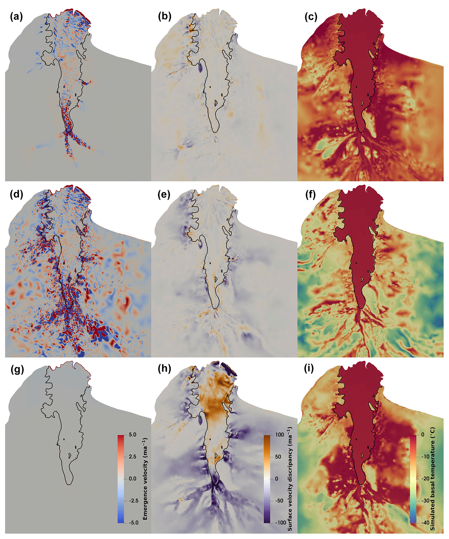
Figure A1The surface emergence velocity (a, d, g), surface horizontal velocity discrepancy (b, e, h) and simulated basal temperature (c, f, i) for simulations E5_c1 (a, b, c), E5_ns (d, e, f) and E5_di (g, h, i) of Gladstone and Wang (2022). The emergence velocity is the surface ice velocity component in the outward normal direction. The surface velocity discrepancy is the difference between simulated and observed surface horizontal velocity.
Figure A1 presents the simulation results of experiment E5 in Gladstone and Wang (2022). In these simulations, the basal dynamic boundary condition for the ice shelf is the same as the present study: the Dirichlet condition on the normal velocity, with the BMB_CAL forcing. For simplicity, the upper surface resistance schemes E5_c2 and E5_c3 are not shown. E5_c1 achieves the best match to the observed surface horizontal velocity field (Fig. A1). For the inland grounded ice, E5_c1 reduces an unrealistic net downward advection of cold ice that occurs with the more natural zero-stress upper surface boundary condition (E5_ns), thus giving a more plausible temperature regime over grounded ice (Fig. A1). In addition, the upper surface resistance described by Eq. (3) is stronger in regions where the observed horizontal velocity is lower, mainly in the interior of the grounded ice sheet. It is close to zero over the ice shelf and thus has very little impact on the dynamics within the ice shelf. Given these considerations, we adopt the E5_c1 upper surface resistance scheme as the dynamic boundary condition in this study.
What we term the ice stiffness factor B(T′), as a function of ice temperature relative to the pressure melting point, is often parameterised by an Arrhenius law form for the ice deformation rate factor (or a pair of matched parameterisations) as
where the included physical parameters (corresponding to the parameters used in our Elmer/Ice simulations) are given by Paterson (1994) and listed in Table B1. The simulated 3-D steady-state temperature field with BMB_CAL has 20 equally spaced layers in the vertical direction. The factor of each layer is calculated at each horizontal grid, and then the depth average calculation is done. The distribution of the calculated depth-averaged temperature-dependent ice stiffness factor is shown in Fig. B1.
Table B1Parameterised physical parameters for the Arrhenius law (Paterson, 1994).
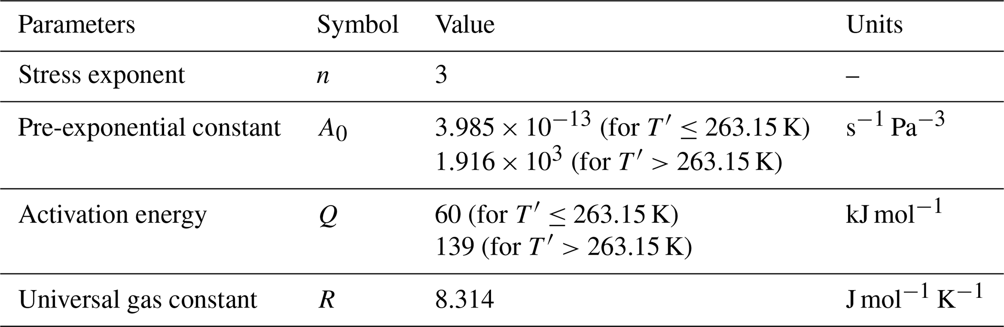
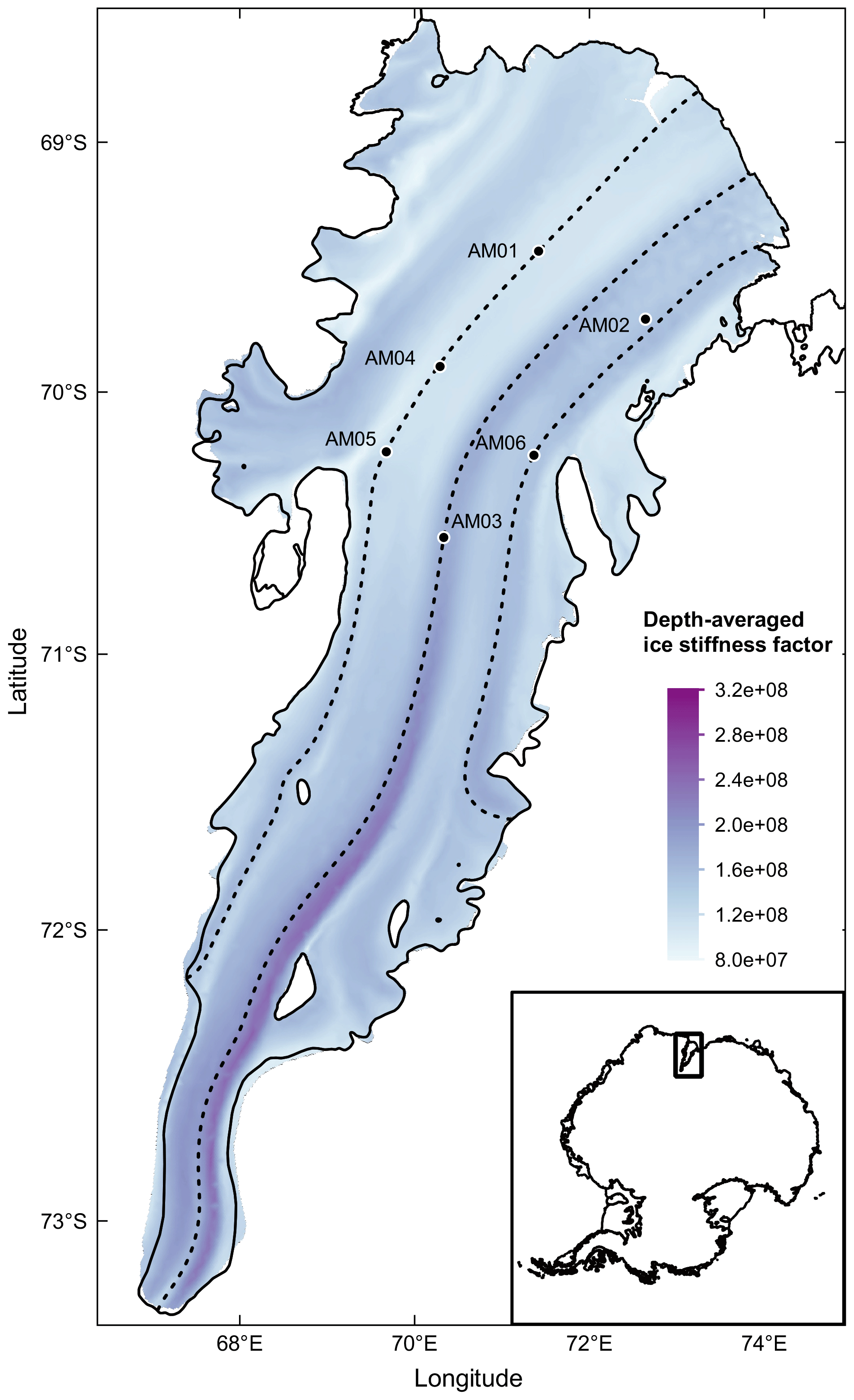
Figure B1Depth-averaged temperature-dependent ice stiffness factor B(T′) (in Pa s) of the AIS derived from the simulated temperature field. Three flowlines, derived from simulated velocity field, are shown with dashed lines. The six boreholes are marked, and the inset shows the location of the Amery Ice Shelf in East Antarctica.
The 3-D full-Stokes model and 1-D free-surface column model are implemented using Elmer/Ice Version: 8.4 (Rev: d296bb) with the code at https://github.com/ElmerCSC/elmerfem.git (Gagliardini et al., 2013). Implementation scripts for the 1-D and 3-D models are available at https://doi.org/10.5281/zenodo.6400721 (Wang, 2022).
We provide the data for the time-averaged borehole temperature profiles (Fig. 6) at https://doi.org/10.5281/zenodo.6406096 (Wang et al., 2022). The borehole internal temperature observations are provided through project AAS 1164 and 4096 maintained by the Australian Antarctic Data Centre (AADC; https://data.aad.gov.au/metadata/records/ASAC_1164, Allison and Craven, 2000). The borehole near-surface temperature data are provided by the automatic weather stations (AWSs) at AM01, AM02 and Amery G3, through project AAS 4506, retrieved from http://aws.cdaso.cloud.edu.au/ (Heil et al., 2022), maintained by the Australian Antarctic Division (AAD).
YW, CZ, BG and RG designed the experiments together. RG implemented the 3-D simulations, and YW implemented the 1-D simulations. YW collated, processed and analysed the original field thermistor data for AM01–AM04, and RW collated, calibrated and analysed the DTS data for AM05–AM06. YW drafted the paper. All authors contributed to the refinement of the experiments, the interpretation of the results and the final paper.
The contact author has declared that neither they nor their co-authors have any competing interests.
Publisher's note: Copernicus Publications remains neutral with regard to jurisdictional claims in published maps and institutional affiliations.
Yu Wang, Chen Zhao, and Ben Galton-Fenzi are supported under the Australian Antarctic Program Partnership (AAPP; Project ID ASCI000002). Yu Wang is also supported by the National Natural Science Foundation of China (no. 41941006). Roland Warner is a University Associate with the AAPP. The Australian Antarctic Program Partnership is led by the University of Tasmania and includes the Australian Antarctic Division, CSIRO Oceans and Atmosphere, Geoscience Australia, the Bureau of Meteorology, the Tasmanian State Government and Australia's Integrated Marine Observing System. Rupert Gladstone is supported by the Academy of Finland (grant no. 322430). This project received grant funding from the Australian Government as part of the Antarctic Science Collaboration Initiative program. We thank Susheel Adusumilli and colleagues for a discussion about marine ice thickness of the Amery Ice Shelf. The AWS data were provided by project AAS 4506 (“Observatory of East Antarctic near-surface atmosphere and cryosphere”). Lastly, we acknowledge the contributions of all the AMISOR field teams and operations support staff and the support of the Australian Antarctic Division through projects AAS 1164 and 4096.
This research has been supported by the Australian Government (grant no. ASCI000002), the National Natural Science Foundation of China (grant no. 41941006) and the Academy of Finland (grant no. 322430).
This paper was edited by Alexander Robinson and reviewed by Thomas Kleiner and one anonymous referee.
Adusumilli, S., Fricker, H. A., Medley, B., Padman, L., and Siegfried, M. R.: Interannual variations in meltwater input to the Southern Ocean from Antarctic ice shelves, Nat. Geosci., 13, 616–620, https://doi.org/10.1038/s41561-020-0616-z, 2020 (data available at https://doi.org/10.6075/J04Q7SHT).
Allison, I.: The AMISOR project: ice shelf dynamics and ice-ocean interaction of the Amery Ice Shelf, FRISP Rep., 14, 1–9, 2003.
Allison, I. and Craven, M.: Ice shelf – ocean interaction in the cavity beneath the Amery Ice Shelf, Ver. 1, Australian Antarctic Data Centre [data set], https://data.aad.gov.au/metadata/records/ASAC_1164 (last access: 1 April 2022), 2000.
Aschwanden, A., Bueler, E., Khroulev, C., and Blatter, H.: An enthalpy formulation for glaciers and ice sheets, J. Glaciol., 58, 441–457, https://doi.org/10.3189/2012JoG11J088, 2012.
Budd, W. F. and Jacka, T. H.: A review of ice rheology for ice sheet modelling, Cold Reg. Sci. Technol., 16, 107–144, https://doi.org/10.1016/0165-232X(89)90014-1, 1989.
Budd, W. F., Corry, M. J., and Jacka, T. H.: Results from the Amery Ice Shelf project, Ann. Glaciol., 3, 36–41, https://doi.org/10.3189/S0260305500002494, 1982.
Buffo, J. J., Schmidt, B. E., and Huber, C.: Multiphase reactive transport and platelet ice accretion in the sea ice of McMurdo Sound, Antarctica, J. Geophys. Res.-Oceans, 123, 324–345, https://doi.org/10.1002/2017JC013345, 2018.
Buffo, J. J., Schmidt, B. E., Huber, C., and Meyer, C. R.: Characterizing the ice-ocean interface of icy worlds: A theoretical approach, Icarus, 360, 114318, https://doi.org/10.1016/j.icarus.2021.114318, 2021.
Comiso, J. C.: Variability and trends in Antarctic surface temperatures from In Situ and satellite infrared measurements, J. Climate, 13, 1674–1696, https://doi.org/10.1175/1520-0442(2000)013<1674:VATIAS>2.0.CO;2, 2000.
Crary, A. P.: Glaciological regime at Little America Station, Antarctica, J. Geophys. Res., 66, 871–878, https://doi.org/10.1029/jz066i003p00871, 1961.
Craven, M., Allison, I., Brand, R., Elcheikh, A., Hunter, J., Hemer, M., and Donoghue, S.: Initial borehole results from the Amery Ice Shelf hot-water drilling project, Ann. Glaciol., 39, 531–539, https://doi.org/10.3189/172756404781814311, 2004.
Craven, M., Carsey, F., Behar, A., Matthews, J., Brand, R., Elcheikh, A., Hall, S., and Treverrow, A.: Borehole imagery of meteoric and marine ice layers in the Amery Ice Shelf, East Antarctica, J. Glaciol., 51, 75–84, https://doi.org/10.3189/172756505781829511, 2005.
Craven, M., Allison, I., Fricker, H. A., and Warner, A. R.: Properties of a marine ice layer under the Amery Ice Shelf, East Antarctica, J. Glaciol., 55, 717–728, https://doi.org/10.3189/002214309789470941, 2009.
Craven, M., Warner, R. C., Galton-Fenzi, B. K., Herraiz-Borreguero, L., Vogel, S. W., and Allison, I.: Platelet ice attachment to instrument strings beneath the Amery Ice Shelf, East Antarctica, J. Glaciol., 60, 383–393, https://doi.org/10.3189/2014JoG13J082, 2014.
Depoorter, M. A., Bamber, J. L., Griggs, J., Lenaerts, J. T. M., Ligtenberg, S. R. M., van den Broeke, M. R., and Moholdt, G.: Antarctic masks (ice-shelves, ice-sheet, and islands), link to shape file, PANGAEA [data set], https://doi.org/10.1594/PANGAEA.819147, 2013.
Dierckx, M. and Tison, J.-L.: Marine ice deformation experiments: an empirical validation of creep parameters, Geophys. Res. Lett., 40, 134–138, https://doi.org/10.1029/2012GL054197, 2013.
Fricker, H. A.: Redefinition of the Amery Ice Shelf, East Antarctica, grounding zone, J. Geophys. Res., 107, 1–9, https://doi.org/10.1029/2001jb000383, 2002.
Fricker, H. A., Popov, S., Allison, I., and Young, N.: Distribution of marine ice beneath the Amery Ice Shelf, Geophys. Res. Lett., 28, 2241–2244, https://doi.org/10.1029/2000GL012461, 2001.
Gagliardini, O., Zwinger, T., Gillet-Chaulet, F., Durand, G., Favier, L., de Fleurian, B., Greve, R., Malinen, M., Martín, C., Råback, P., Ruokolainen, J., Sacchettini, M., Schäfer, M., Seddik, H., and Thies, J.: Capabilities and performance of Elmer/Ice, a new-generation ice sheet model, Geosci. Model Dev., 6, 1299–1318, https://doi.org/10.5194/gmd-6-1299-2013, 2013.
Galton-Fenzi, B. K., Maraldi, C., Coleman, R., and Hunter, J.: The cavity under the Amery Ice Shelf, East Antarctica, J. Glaciol., 54, 881–887, https://doi.org/10.3189/002214308787779898, 2008.
Galton-Fenzi, B. K., Hunter, J. R., Coleman, R., Marsland, S. J., and Warner, R. C.: Modeling the basal melting and marine ice accretion of the Amery Ice Shelf, J. Geophys. Res.-Ocean., 117, 1–19, https://doi.org/10.1029/2012JC008214, 2012.
Gillet-Chaulet, F., Gagliardini, O., Seddik, H., Nodet, M., Durand, G., Ritz, C., Zwinger, T., Greve, R., and Vaughan, D. G.: Greenland ice sheet contribution to sea-level rise from a new-generation ice-sheet model, The Cryosphere, 6, 1561–1576, https://doi.org/10.5194/tc-6-1561-2012, 2012.
Gladstone, R. and Wang, Y.: Antarctic regional inversions using Elmer/Ice: methodology, Zenodo, https://doi.org/10.5281/ZENODO.5862046, 2022.
Glen, J. W.: The flow law of ice: A discussion of the assumptions made in glacier theory, their experimental foundations and consequences, IASH Publ., 47, 171–183, 1958.
Greve, R.: A continuum-mechanical formulation for shallow polythermal ice sheets, Philos. T. R. Soc. Lond. A 355, 921–974, 1997.
Greve, R., Calov, R., Obase, T., Saito, F., Tsutaki, S., and Abe-Ouchi, A.: ISMIP6 future projections for the Antarctic ice sheet with the model SICOPOLIS, Zenodo, https://doi.org/10.5281/ZENODO.4035932, 2020.
Heil, P., Hyland, G., and Allison, I.: : Observatory of East Antarctic near-surface atmosphere and cryosphere, http://aws.cdaso.cloud.edu.au/, last access: 31 March 2022.
Herraiz-Borreguero, L., Allison, I., Craven, M., Nicholls, K. W. and Rosenberg, M. A.: Ice shelf/ocean interactions under the Amery Ice Shelf: Seasonal variability and its effect on marine ice formation, J. Geophys. Res.-Ocean., 118, 7117–7131, https://doi.org/10.1002/2013JC009158, 2013.
Humbert, A.: The temperature regime of Fimbulisen, Antarctica, Ann. Glaciol., 51, 56–64, https://doi.org/10.3189/172756410791392673, 2010.
Jania, J., Mochnacki, D., and Gdek, B.: The thermal structure of Hansbreen, a tidewater glacier in southern Spitsbergen, Svalbard, Polar Res., 15, 53–66, https://doi.org/10.3402/polar.v15i1.6636, 1996.
Jourdain, N. C., Asay-Davis, X., Hattermann, T., Straneo, F., Seroussi, H., Little, C. M., and Nowicki, S.: A protocol for calculating basal melt rates in the ISMIP6 Antarctic ice sheet projections, The Cryosphere, 14, 3111–3134, https://doi.org/10.5194/tc-14-3111-2020, 2020.
Khazendar, A., Rignot, E., and Larour, E.: Roles of marine ice, rheology, and fracture in the flow and stability of the Brunt/Stancomb-Wills Ice Shelf, J. Geophys. Res.-Earth, 114, F04007, https://doi.org/10.1029/2008JF001124, 2009.
King, M. A., Coleman, R., Morgan, P. J., and Hurd, R. S.: Velocity change of the Amery Ice Shelf, East Antarctica, during the period 1968–1999, J. Geophys. Res., 112, F01013, https://doi.org/10.1029/2006JF000609, 2007.
Kobs, S., Holland, D. M., Zagorodnov, V., Stern, A., and Tyler, S. W.: Novel monitoring of Antarctic ice shelf basal melting using a fiber-optic distributed temperature sensing mooring, Geophys. Res. Lett., 41, 6779–6786, https://doi.org/10.1002/2014GL061155, 2014.
Kobs, S. B.: In situ temperature monitoring of the McMurdo Ice Shelf and ice shelf cavity by fiber-optic distributed temperature sensing, Doctoral thesis, http://hdl.handle.net/11714/2917 (last access: 5 April 2022), 2014.
Kulessa, B., Jansen, D., Luckman, A. J., King, E. C., and Sammonds, P. R.: Marine ice regulates the future stability of a large Antarctic ice shelf, Nat. Commun., https://doi.org/10.1038/ncomms4707, 2014.
Lambrecht, A., Sandhäger, H., Vaughan, D. G. and Mayer, C.: New ice thickness maps of Filchner-Ronne Ice Shelf, Antarctica, with specific focus on grounding lines and marine ice, Antarct. Sci., 19, 521–532, https://doi.org/10.1017/S0954102007000661, 2007.
Lewis, E. L. and Perkin, R. G.: Ice pumps and their rates, J. Geophys. Res., 91, 11756–11762, https://doi.org/10.1029/jc091ic10p11756, 1986.
Macayeal, D. R. and Thomas, R. H.: Ross Ice Shelf temperatures support a history of ice-shelf thickening, Nature, 282, 703–705, https://doi.org/10.1038/282703a0, 1979.
Makinson, K.: BAS hot water drilling on Ronne Ice Shelf, Antarctica, Mem. Natl. Inst. Polar Res. Spec. issue, 49, 192–202, 1994.
Martos, Y. M., Catalán, M., Jordan, T. A., Golynsky, A., Golynsky, D., Eagles, G. and Vaughan, D. G.: Heat Flux Distribution of Antarctica Unveiled, Geophys. Res. Lett., 44, 11417–11426, https://doi.org/10.1002/2017GL075609, 2017.
McDougall, T. J., Barker, P. M., Feistel, R., and Galton-Fenzi, B. K.: Melting of ice and sea ice into seawater and frazil ice formation, J. Phys. Oceanogr., 44, 1751–1775, https://doi.org/10.1175/JPO-D-13-0253.1, 2014.
Morlighem, M.: MEaSUREs BedMachine Antarctica, Version 1. Boulder, Colorado USA, NASA National Snow and Ice Data Center Distributed Active Archive Center [data set], https://doi.org/10.5067/C2GFER6PTOS4, 2019.
Morlighem, M., Rignot, E., Seroussi, H., Larour, E., Ben Dhia, H., and Aubry, D.: Spatial patterns of basal drag inferred using control methods from a full-Stokes and simpler models for Pine Island Glacier, West Antarctica, Geophys. Res. Lett., 37, L14502, https://doi.org/10.1029/2010GL043853, 2010.
Morlighem, M., Rignot, E., Binder, T., Blankenship, D. D., Drews, R., Eagles, G., Eisen, O., Ferraccioli, F., Forsberg, R., Fretwell, P., Goel, V., Greenbaum, J. S., Gudmundsson, H., Guo, J., Helm, V., Hofstede, C., Howat, I., Humbert, A., Jokat, W., Karlsson, N. B., Lee, W., Matsuoka, K., Millan, R., Mouginot, J., Paden, J., Pattyn, F., Roberts, J. L., Rosier, S., Ruppel, A., Seroussi, H., Smith, E. C., Steinhage, D., Sun, B., van den Broeke, M. R., van Ommen, T., van Wessem, M., and Young, D. A.: Deep glacial troughs and stabilizing ridges unveiled beneath the margins of the Antarctic ice sheet, Nat. Geosci., 13, 132–137, https://doi.org/10.1038/s41561-019-0510-8, 2020.
Orheim, O., Hagen, J. O., Østerhus, S., and Saetrang, A. C.: Glaciologic and oceanographic studies on Fimbulisen during NARE 1989/90, FRISP Rep, 4, 120–131, 1990a.
Orheim, O., Hagen, J. O., Østerhus, S., and Sœtrang, A. C.: Studies on, and underneath, the ice shelf Fimbulisen, Nor. Polarinstitutt Meddelelser, 113, 59–73, 1990b.
Paterson, W. S. B.: The physics of glaciers, 3rd Edn., Oxford, Elsevier, 1994.
Pittard, M. L., Roberts, J. L., Watson, C. S., Galton-Fenzi, B. K., Warner, R. C., and Coleman, R.: Velocities of the Amery Ice Shelf's primary tributary glaciers, 2004–12, Antarct. Sci., 27, 511–523, https://doi.org/10.1017/S0954102015000231, 2015.
Pittard, M. L., Galton-Fenzi, B. K., Watson, C. S., and Roberts J. L.: Future sea level change from Antarctica's Lambert-Amery glacial system, Geophys. Res. Lett., 44, 7347–7355, https://doi.org/10.1002/2017GL073486, 2017.
Rignot, E., Mouginot, J., and Scheuchl, B.: MEaSUREs InSAR-Based Antarctica Ice Velocity Map, Version 2, Boulder, Color., USA, NASA Natl. Snow Ice Data Cent. Distrib. Act. Arch. Center [data set], https://doi.org/10.5067/D7GK8F5J8M8R, 2017.
Ritz, C.: Time dependent boundary conditions for calculation of temperature fields in ice sheets, IAHS Publ., 170, 207–216, 1987.
Ryser, C.: Cold ice in an alpine glacier and ice dynamics at the margin of the Greenland Ice Sheet, Doctoral thesis, ETH Zurich, https://doi.org/10.3929/ethz-a-010129038, 2014.
Saito, F. and Abe-Ouchi, A.: Thermal structure of Dome Fuji and east Dronning Maud Land, Antarctica, simulated by a three-dimensional ice-sheet model, Ann. Glaciol., 39, 433–438, https://doi.org/10.3189/172756404781814258, 2004.
Schoof, C. and Hewitt, I. J.: A model for polythermal ice incorporating gravity-driven moisture transport, J. Fluid. Mech., 797, 505–535, https://doi.org/10.1017/jfm.2016.251, 2016.
Seroussi, H., Morlighem, M., Rignot, E., Khazendar, A., Larour, E., and Mouginot, J.: Dependence of century-scale projections of the Greenland ice sheet on its thermal regime, J. Glaciol., 59, 1024–1034, https://doi.org/10.3189/2013JoG13J054, 2013.
Seroussi, H., Nowicki, S., Payne, A. J., Goelzer, H., Lipscomb, W. H., Abe-Ouchi, A., Agosta, C., Albrecht, T., Asay-Davis, X., Barthel, A., Calov, R., Cullather, R., Dumas, C., Galton-Fenzi, B. K., Gladstone, R., Golledge, N. R., Gregory, J. M., Greve, R., Hattermann, T., Hoffman, M. J., Humbert, A., Huybrechts, P., Jourdain, N. C., Kleiner, T., Larour, E., Leguy, G. R., Lowry, D. P., Little, C. M., Morlighem, M., Pattyn, F., Pelle, T., Price, S. F., Quiquet, A., Reese, R., Schlegel, N.-J., Shepherd, A., Simon, E., Smith, R. S., Straneo, F., Sun, S., Trusel, L. D., Van Breedam, J., van de Wal, R. S. W., Winkelmann, R., Zhao, C., Zhang, T., and Zwinger, T.: ISMIP6 Antarctica: a multi-model ensemble of the Antarctic ice sheet evolution over the 21st century, The Cryosphere, 14, 3033–3070, https://doi.org/10.5194/tc-14-3033-2020, 2020.
Treverrow, A., Warner, R. C., Budd, W. F., and Craven, M.: Meteoric and marine ice crystal orientation fabrics from the amery ice shelf, East Antarctica, J. Glaciol., 56, 877–890, https://doi.org/10.3189/002214310794457353, 2010.
Tyler, S. W., Holland, D. M., Zagorodnov, V., Stern, A. A., Sladek, C., Kobs, S., White, S., Suárez, F., and Bryenton, J.: Using distributed temperature sensors to monitor an Antarctic ice shelf and sub-ice-shelf cavity, J. Glaciol., 59, 583–591, https://doi.org/10.3189/2013JoG12J207, 2013.
van Wessem, J. M., van de Berg, W. J., Noël, B. P. Y., van Meijgaard, E., Amory, C., Birnbaum, G., Jakobs, C. L., Krüger, K., Lenaerts, J. T. M., Lhermitte, S., Ligtenberg, S. R. M., Medley, B., Reijmer, C. H., van Tricht, K., Trusel, L. D., van Ulft, L. H., Wouters, B., Wuite, J., and van den Broeke, M. R.: Modelling the climate and surface mass balance of polar ice sheets using RACMO2 – Part 2: Antarctica (1979–2016), The Cryosphere, 12, 1479–1498, https://doi.org/10.5194/tc-12-1479-2018, 2018.
Wang, Y.: yuwang115/1D-and-3D-model-for-LAGs: 3D and 1D models for the temperature simulations of the LAGs (Version version1), Zenodo [code], https://doi.org/10.5281/zenodo.6400721, 2022.
Wang, Y., Zhao, C., Gladstone, R., Galton-Fenzi, B., and Warner, R.: Time-averaged borehole temperatures at AM01–AM06 on the Amery Ice Shelf (Version 1), Zenodo [data set], https://doi.org/10.5281/zenodo.6406096, 2022.
Warner, R. C., Craven, M., Galton-Fenzi, B., Elcheikh, A., Christensen, A. and Vogel, S. W.: Distributed temperature sensing in the Amery Ice shelf and the sub ice shelf ocean, in: . Book of Abstracts of 26th International Forum for Research into Ice Shelf Processes (FRISP), edited by: Hanke, M. and Kirchner, N., 12–14 June 2012, Stockholm Archipelago, Sweden http://urn.kb.se/resolve?urn=urn:nbn:se:su:diva-88405 (last access: 5 April 2022), 2012.
Wexler, H.: Heating and Melting of Floating Ice Shelves, J. Glaciol., 3, 626–645, https://doi.org/10.3189/s0022143000023741, 1960.
Yu, J., Liu, H., Jezek, K. C., Warner, R. C., and Wen, J.: Analysis of velocity field, mass balance, and basal melt of the Lambert glacier-amery ice shelf system by incorporating Radarsat SAR interferometry and ICESat laser altimetry measurements, J. Geophys. Res.-Sol. Ea., 115, B11102, https://doi.org/10.1029/2010JB007456, 2010.
- Abstract
- Introduction
- Data and methods
- Results
- Discussion
- Conclusions
- Appendix A: Upper surface dynamic boundary condition
- Appendix B: Calculation of the depth-averaged ice stiffness factor
- Code availability
- Data availability
- Author contributions
- Competing interests
- Disclaimer
- Acknowledgements
- Financial support
- Review statement
- References