Generating large-scale sea ice motion from Sentinel-1 and the RADARSAT Constellation Mission using the Environment and Climate Change Canada automated sea ice tracking system

As Arctic sea ice extent continues to decline, remote sensing observations are becoming even more vital for the monitoring and understanding of sea ice. Recently, the sea ice community has entered a new era of synthetic aperture radar (SAR) satellites operating at C-band with the launch of Sentinel-1A in 2014 and Sentinel-1B (S1) in 2016 and the RADARSAT Constellation Mission (RCM) in 2019. These missions represent five spaceborne SAR sensors that together routinely cover the pan-Arctic sea ice domain. Here, we describe, apply, and validate the Environment and Climate Change Canada automated sea ice tracking system (ECCC-ASITS) that routinely generates large-scale sea ice motion (SIM) over the pan-Arctic domain using SAR images from S1 and RCM. We applied the ECCC-ASITS to the incoming image streams of S1 and RCM from March 2020 to October 2021 using a total of 135 471 SAR images and generated new SIM datasets (7 d 25 km and 3 d 6.25 km) by combining the image stream outputs of S1 and RCM (S1 + RCM). Results indicate that S1 + RCM SIM provides more coverage in the Hudson Bay, Davis Strait, Beaufort Sea, Bering Sea, and directly over the North Pole compared to SIM from S1 alone. Based on the resolvable S1 + RCM SIM grid cells, the 7 d 25 km spatiotemporal scale is able to provide the most complete picture of SIM across the pan-Arctic from SAR imagery alone, but considerable spatiotemporal coverage is also available from 3 d 6.25 SIM products. S1 + RCM SIM is resolved within the narrow channels and inlets of the Canadian Arctic Archipelago, filling a major gap from coarser-resolution sensors. Validating the ECCC-ASITS using S1 and RCM imagery against buoys indicates a root-mean-square error (RMSE) of 2.78 km for dry ice conditions and 3.43 km for melt season conditions. Higher speeds are more apparent with S1 + RCM SIM as comparison with the National Snow and Ice Data Center (NSIDC) SIM product and the Ocean and Sea Ice Satellite Application Facility (OSI SAF) SIM product indicated an RMSE of u=4.6 km d⁻¹ and v=4.7 km d⁻¹ for the NSIDC and u=3.9 km d⁻¹ and v=3.9 km d⁻¹ for OSI SAF. Overall, our results demonstrate the robustness of the ECCC-ASITS for routinely generating large-scale SIM entirely from SAR imagery across the pan-Arctic domain.

1 Introduction

As Arctic sea ice extent continues to decline in concert with increases in carbon dioxide (CO₂) emissions (Notz and Stroeve, 2016), remote sensing observations are becoming even more vital for the monitoring and understanding of Arctic sea ice. Recently, the sea ice community has entered a new era of synthetic aperture radar (SAR) satellites operating at C-band (wavelength, λ=5.5 cm) with the launch of Sentinel-1A in 2014, Sentinel-1B in 2016 (S1; Torres et al., 2012), and the RADARSAT Constellation Mission (RCM) in 2019 (Thompson, 2015). Together these missions represent five spaceborne SAR sensors that when combined offer the opportunity to retrieve large-scale sea ice geophysical variables with high spatiotemporal resolution. An important sea ice geophysical variable that could benefit from large-scale SAR estimates across the Arctic is sea ice motion (SIM). SIM is controlled by the exchange of momentum due to a turbulent process primarily from atmospheric and oceanic forcing. Away from the coast, winds explain 70 % or more of the variance in Arctic sea ice motion (Thorndike and Colony, 1982), and as a result, monitoring changes in SIM is important for understanding how sea ice responds to changes in atmospheric circulation (Rigor et al., 2002). SIM convergent and divergent processes impact the overall thickness of Arctic sea ice (Kwok, 2015), and the dynamic component of the Arctic sea ice area and volume balance is also impacted by SIM (Kwok, 2004, 2009). The long-term record of SIM in the Arctic indicates the ice speed is increasing, which is associated with thinner ice being more susceptible to wind forcing (Rampal et al., 2009; Kwok et al., 2013; Moore et al., 2019).

Techniques for estimating SIM from satellite observations have a long history dating back to the late 1980s and early 1990s and are primarily based on the maximum cross-correlation coefficient between overlapping images (e.g., Fily and Rothrock, 1990; Kwok et al., 1990; Emery et al., 1991). The maximum cross-correlation approach to estimate SIM can be applied to virtually any overlapping pair of satellite imagery separated by a relatively short time interval of ∼1–3 d. For large-scale SIM, passive microwave imagery is typically the most widely used because of its large swath and daily coverage (e.g., Agnew et al., 1997; Kwok et al., 1998; Lavergne et al., 2010; Tschudi et al., 2020). Enhanced-resolution SIM products with spatial resolutions of ∼2 km have also been generated (e.g., Haarpaintner, 2006; Agnew et al., 2008), although they have not been widely utilized. The limitation with respect to large-scale SIM estimated from passive microwave imagery, however, is a low spatial resolution (50–100 km). As a result, SIM is more difficult to track with lower-spatial-resolution passive microwave sensors (Kwok et al., 1998) especially within narrow channels and inlets (e.g., the Canadian Arctic Archipelago; CAA) compared to SAR. However, SIM estimates from SAR are typically regionally based because of image availability across the Arctic. With the availability of SAR imagery from S1 and RCM, a new opportunity exists to provide both the operational and scientific communities with larger-scale estimates of SIM from SAR. In addition, with marine activity in the Arctic increasing (e.g., Eguíluz et al., 2016; Dawson et al., 2018), a wide range of maritime stakeholders could benefit from access to large-scale SAR SIM for safety, planning, and situational awareness (Wagner et al., 2020).

In this study, we describe, apply, and validate the Environment and Climate Change Canada automated sea ice tracking system (ECCC-ASITS) using SAR imagery from the S1 and RCM to generate new SIM products over the pan-Arctic domain. Prior to S1 there was a lack of widely available SAR imagery for pan-Arctic SIM generation, and as a result, this is perhaps the first time such an extensive processing of SAR imagery at the pan-Arctic scale has been undertaken to generate SIM. The ECCC-ASITS is designed to facilitate the routine generation of SIM to serve operations within ECCC and provide new and unique SIM data to the wider scientific community and maritime stakeholders. Here, we focus primarily on the latter applications by first describing the ECCC-ASITS workflow that produces SIM from S1 and RCM SAR imagery (hereafter, S1 + RCM) in close to near real time and combines the output into S1 + RCM SIM products. A close to near-real-time workflow is required given the considerable amount of incoming SAR imagery together with the computational time to generate SIM. We then present the results of two S1 + RCM products from March 2020 to October 2021 followed by a section discussing the validation and uncertainty of S1 + RCM SIM products. Finally, we provide a comparison of our S1 + RCM SIM to the existing SIM datasets from the National Snow and Ice Data Center (NSIDC) (Tschudi et al., 2020) and Ocean and Sea Ice Satellite Application Facility (OSI SAF) SIM (Lavergne et al., 2010).

2 Data

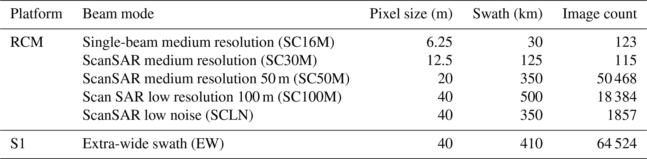
The primary datasets used in this analysis were extra-wide-swath imagery at HH polarization from S1 and ScanSAR medium resolution 50 m (SC50M), ScanSAR low resolution 100 m (SC100M), and ScanSAR low noise (SCLN) at HH polarization from RCM from March 2020 to April 2021 (Table 1). We also used daily buoy positions from International Arctic Buoy Programme (IABP) for April and August 2020 and 2021, the 7 d 25 km SIM NSIDC Polar Pathfinder dataset, and the 2 d multi-sensor low resolution 62.5 km OSI SAF sea ice motion dataset (OSI-405) from March to December 2020. Tschudi et al. (2020) provides a complete description of the NSIDC Polar Pathfinder SIM dataset, and Lavergne et al. (2010) provides a complete description of the OSI SAF SIM dataset. Finally, we used daily pan-Arctic ice charts from the National Ice Center for 2020 and 2021.

Table 1 Satellite SAR image inventory used in this analysis from March 2020 to October 2021.

3 Methods

3.1 ECCC automated sea ice tracking algorithm

We make use of the automated SIM tracking algorithm developed by Komarov and Barber (2014) to estimate large-scale SIM across the pan-Arctic domain. The algorithm has been widely utilized for applications that require robust estimates of SIM in the Arctic using SAR at C-band (e.g., Howell et al., 2013, 2018; Komarov and Buehner, 2019; Moore et al., 2021b). A full description is provided by Komarov and Barber (2014), but the main components of the algorithm are briefly described here. To begin with, coarser-spatial-resolution images are generated from the original spatial resolution of the SAR image pairs. For example, if the original SAR image pairs have a spatial resolution of 200 m, then the additional generated levels would be 400 and 800 m. A set of control points (i.e., ice features) is automatically generated for each resolution level based on the SAR image local variances. To highlight edges and heterogeneities at each resolution level, a Gaussian filter and the Laplace operator are applied sequentially. Beginning with the coarsest resolution level, ice feature matches in the image pairs are identified by combining the phase-correlation and cross-correlation matching techniques that allow for both the translation and rotational components of SIM to be identified. SIM vectors not presented in both forward and backwards image registration passes are filtered out, as well as vectors with low cross-correlation coefficients. In order to refine the SIM vectors, at each consecutive resolution level the algorithm is guided by SIM vectors identified at the previous resolution. An example of the SIM output generated from the algorithm based on two overlapping SAR images is shown in Fig. 1. The limitations that are widely known with respect to estimating SIM from SAR imagery including regions of low ice concentration, melt water on the surface of the sea ice, and longer time separation between images also apply to this algorithm.

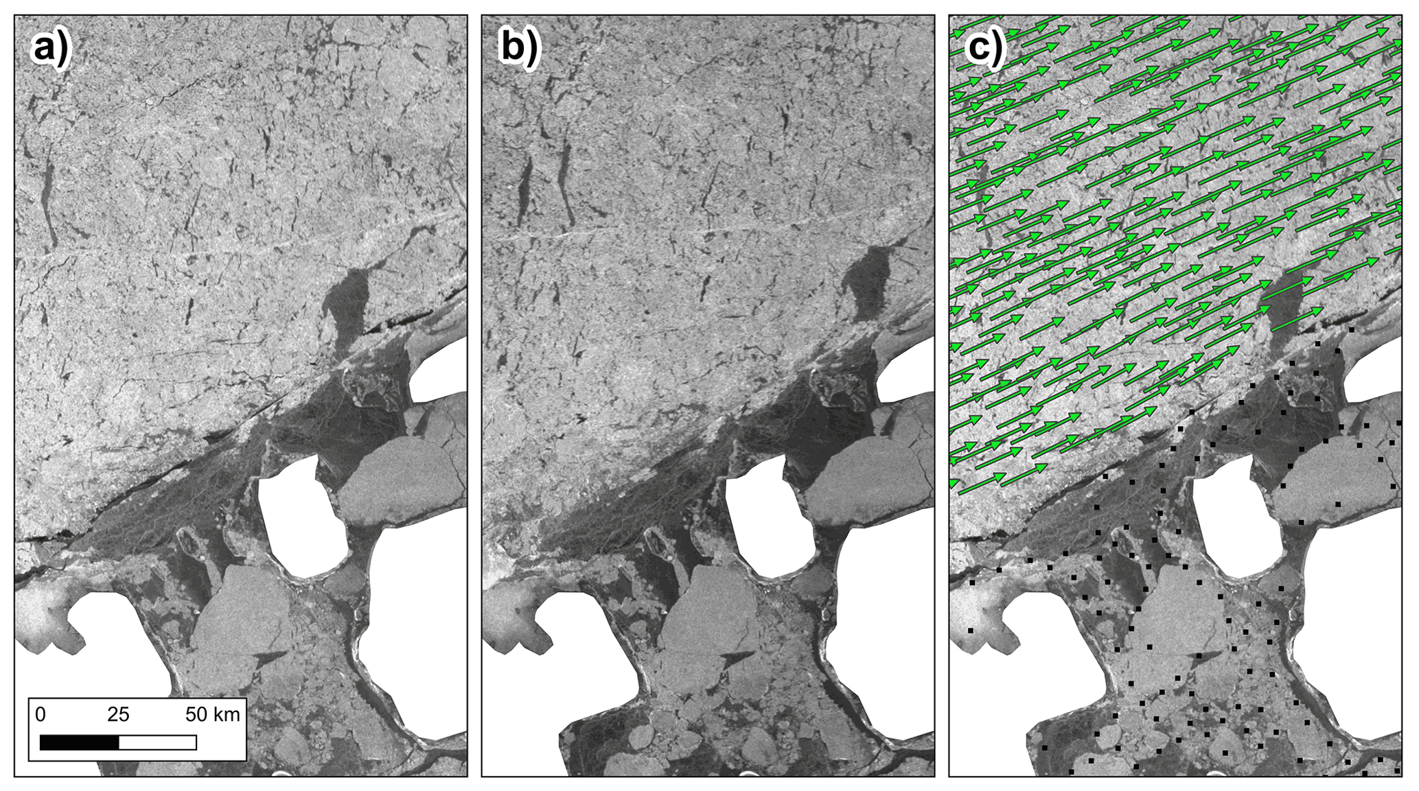
Figure 1 (a) RCM image on 7 April 2020, (b) RCM image on 10 April 2020, and (c) detected sea ice motion vectors (green) over RCM 7 April 2020. The black dots indicate detection vectors with no motion. RADARSAT Constellation Mission imagery © Government of Canada 2020. RADARSAT is an official mark of the Canadian Space Agency.

3.2 ECCC automated sea ice tracking system (ECCC-ASITS)

The ECCC-ASITS facilitates the routine generation of S1 + RCM SIM products; however, it should be noted the system has roots (i.e., it has been built up) in previous studies (e.g., Howell and Brady, 2019; Babb et al., 2021; Moore et al., 2021a, b). While the primary system methodology described here is for larger-scale SIM generation, it is not strictly limited for this application and can be (has been) modified to accommodate specific objectives.

The generalized processing chain for generating large-scale S1 + RCM SIM using ECCC-ASITS is illustrated in Fig. 2. The approach processes the S1 and RCM image streams separately and then combines the outputs into a S1 + RCM SIM product. This parallel approach was chosen for several reasons. First, mixing S1 and RCM primarily improves spatial coverage as RCM mainly fills in the spatial gaps in S1 coverage. Specifically, RCM coverage is more widely spread across the Arctic and covering the Bering Sea, Laptev Sea, Davis Strait, southern Beaufort Sea, and even the North Pole, thus filling a gap typically associated with the majority of satellite sensors (Fig. 3). An example of the ability of RCM to almost completely cover the North Pole on a single day is shown in Fig. 4. However, we note that the temporal resolution of SIM could be improved by mixing S1 and RCM, but this would be restricted to only certain regions of the Arctic. Second, SAR imagery is received by ECCC from S1 and RCM in close to near real time and in order to “keep up” with the hundreds of images coming in per day and routinely generate products every day the processing system is run every hour given the computational load on automated SIM detection. Figure 5 illustrates the amount of S1 and RCM SAR imagery that was processed over a 7 d time period in March 2020, which amounted to over 1132 SAR images or ∼160 images per day. Finally, different orbit characteristics of the satellites contribute to timing differences between when the images are acquired compared to when they are received by ECCC. For example, if an S1 image acquired at 13:00 UTC were transferred to our system sooner than an RCM image that was acquired at 11:00 UTC, then the RCM image would be missed. We note that S1A and S1B are freely mixed in the Sentinel processing chain, and RCM1, RCM2, and RCM3 are mixed in the RCM processing chain.

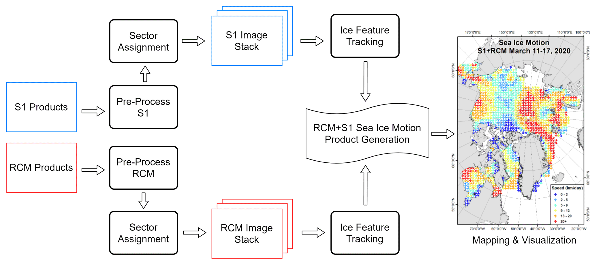
Figure 2 Generalized processing chain for generating large-scale sea ice motion from S1 and RCM across the pan-Arctic domain.

Figure 3 Image density per week for (a) S1, (b) RCM, and (c) S1 + RCM based on Table 1.

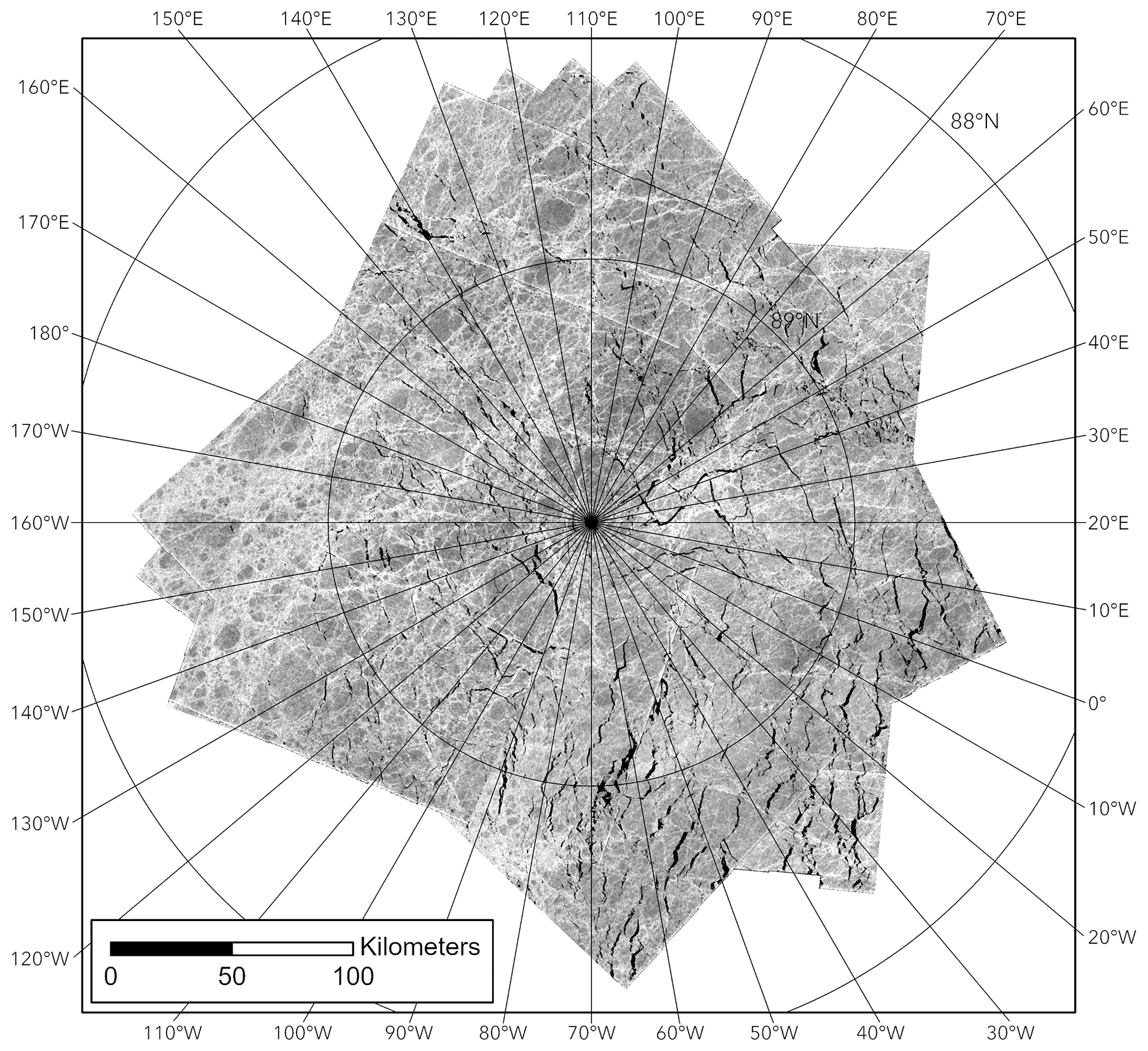
Figure 4 RCM image coverage over the North Pole on 15 September 2020. RADARSAT Constellation Mission imagery © Government of Canada 2020. RADARSAT is an official mark of the Canadian Space Agency.

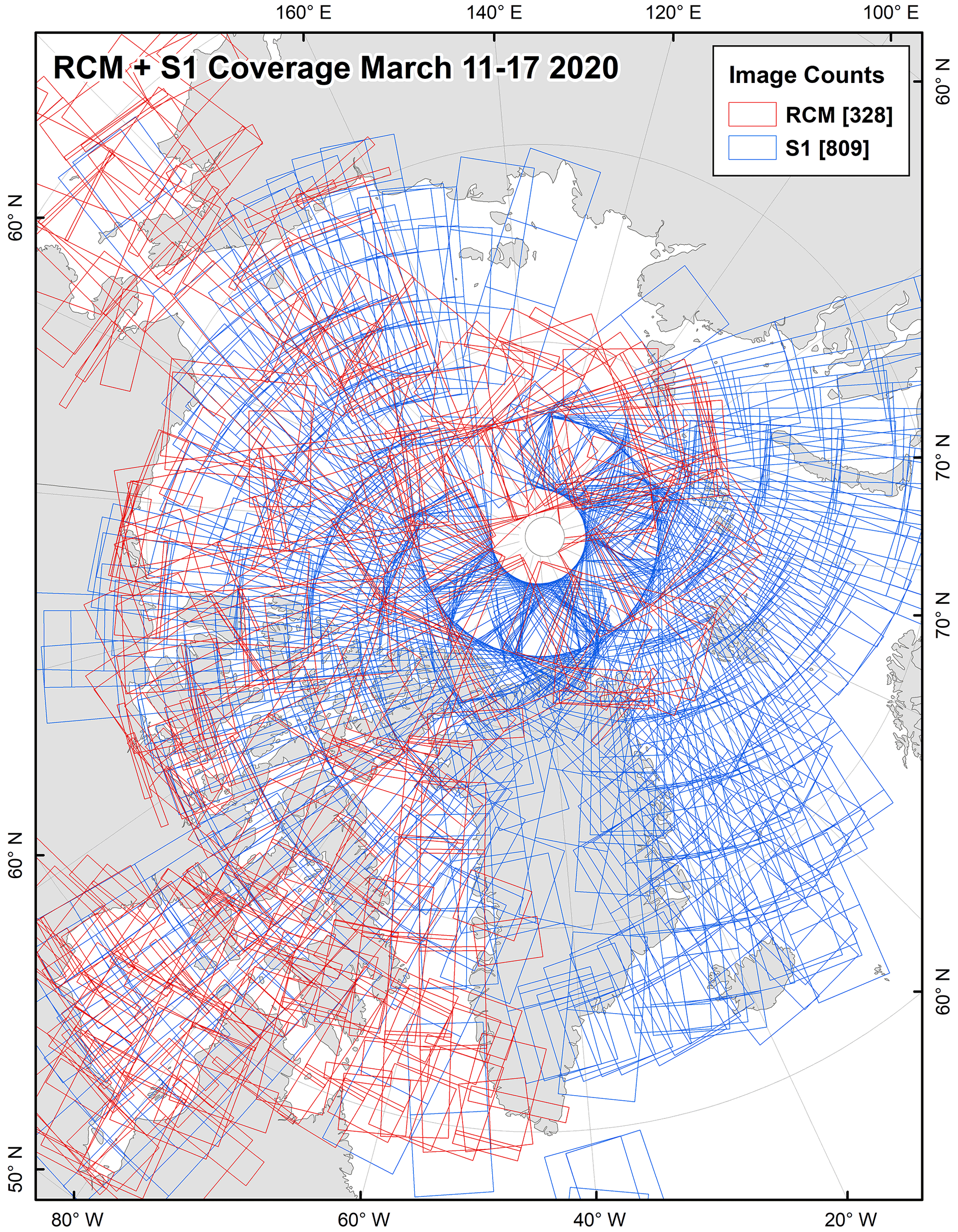
Figure 5 Spatial distribution of S1 and RCM SAR images from 11–17 March 2020.

For both S1 and RCM image streams, the pre-processing steps shown in Fig. 2 first involve calibrating the imagery to the backscatter coefficient of sigma nought (σ^∘) using the HH-polarization channel and map projected to the NSIDC North Pole stereographic WGS-84, EPSG:3413 coordinate system with a 200 m pixel size. For S1 imagery, pre-processing steps were applied using the Graph Processing Tool (GPT) of the Sentinel Application Platform (SNAP) software, and for RCM imagery, the pre-processing workflow was applied using an in-house pre-processor.

Manual inspection of SAR imagery and subsequent image stack compilation prior to automatic SIM generation, while effective in regional-scale studies (e.g., Howell et al., 2013, 2016; Moore et al., 2021b), is not practical for generating large-scale SIM. The main challenges of estimating large-scale SIM across the pan-Arctic domain are (i) handling the large volume and delivery frequency of the imagery, (ii) efficiently selecting image stacks, and (iii) providing more computationally efficient feature tracking from the image stacks.

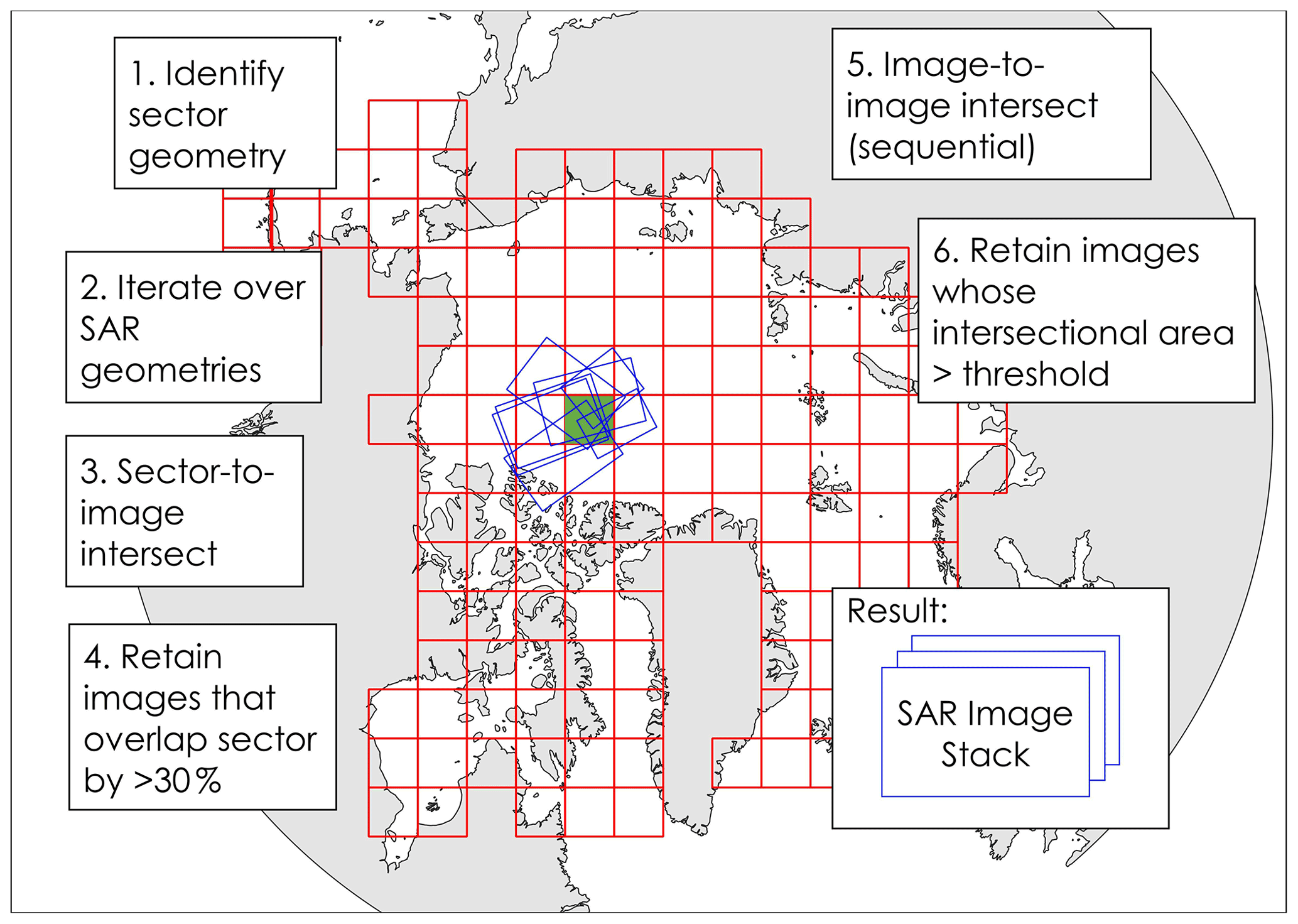
Figure 6 Processing steps for automatically generating the S1 or RCM synthetic aperture radar (SAR) image stack selection.

To address (i) and (ii), an automated approach for determining the suitability of images for inclusion in the automatic SIM generation (i.e., S1 or RCM image stack selection) was developed and depicted in Fig. 6. For the image stack selection, a 400 km × 400 km grid of sectors encompassing the pan-Arctic was generated and used to create overlapping stacks of SAR image pairs (Fig. 6). The footprint geometry of each SAR image was compared to a given sector's extent, and if the overlap was greater than 30 %, that image was retained for feature tracking. Next, we assess image-to-image overlap within each sector to create a temporally sequential stack of images that intersected one another to an acceptable degree (≥32 000 km²). Images within each sector with an overlap of at least 32 000 km² were retained for feature tracking. The stacks are created every hour using the last-processed image from the previous run and the accumulated new imagery that had arrived in the time preceding.

For (iii), a more computationally efficient application of automatic SIM tracking algorithm (i.e., image stack processing) was developed. Traditionally, image stacks were processed serially, which was effective for local-scale studies with limited amounts of imagery, but with significant increases in the SAR image data volume and study area domain size from S1 and RCM, it was necessary to enhance the processing speed of ice feature tracking analysis. The concurrent approach as outlined in Fig. 7 takes advantage of vertical scalability by increasing the number of processes during image pair analysis. This approach allowed for an entire image stack to be efficiently processed with as many computational cores as were available. For example, when three sets of image pairs are processing and process 3 finishes before process 2, process 3 picks up the next sequence of pairs instead of waiting for process 2 (Fig. 7). After stack processing, the last-processed image for the given sector is recorded in a database and processing ends. It is important to note there is currently no “staleness” limit for the SAR images in a given sector. There are occasionally instances when long stretches of time (e.g., 7 d) occur between image pairs, but this is mostly confined to the edge sectors of the grid. Unfortunately, the computational capacity to take on the additional processing load of using the same image in multiple pair combinations is not currently available in the infrastructure being used.

Figure 7 Illustration of the horizontal scalability approach used to process S1 or RCM image stacks.

The final step involves combining the results of the automatic S1 and RCM SIM tracking process into defined spatial and temporal resolution grids to be used for analysis and mapping (Fig. 2). Combining the SIM output from S1 with RCM (i.e., S1 + RCM) facilitates the ability to improve the spatial coverage because of S1 + RCM image density across the Arctic (Fig. 3). In addition, S1 + RCM image density generally increases with latitude (Fig. 3), indicating that more consistent coverage of the ice pack will be possible during the melt season, which is beneficial considering this is when automated SIM tracking algorithms have more difficulty. Two datasets are routinely produced: 7 d 25 km and 3 d (rolling) 6.25 km. The former is to represent a spatially complete picture of SIM generated from SAR and the latter to provide a higher-resolution dataset that can benefit applications requiring higher spatiotemporal resolution. It should be noted that, based on S1 + RCM image density shown in Fig. 3, regional S1 + RCM SIM products at higher spatial and temporal resolution are certainly achievable and ECCC-ASITS can be modified to produce SIM to very localized studies (e.g., Moore et al., 2021a, b).

For each grid cell, at least five individually tracked SIM vectors had to be within a distance of 3 times the grid cell resolution cell centroid. Considering the SIM vectors are determined at a spatial resolution of 200 m and gridding takes place at 25 and 6.25 km, numerous vectors are within the grid cell. Only SIM vectors estimated from image pairs with a time separation of greater than 12 h were considered. We selected a 12 h cut-off because below 12 h the SIM resulted in less representative results, often due to higher wind speeds with respect to the averaged product value (over 3 or 7 d). This was the primary observation from previous studies constructing a very high temporal resolution time series (e.g., Howell and Brady, 2019; Moore et al., 2021b). Use of ice displacement vectors derived from images with lower time separation (<12 h) would lead to less representative (more uncertain) average ice speeds in 3 or 7 d average SIM products. In addition, SIM vectors with speeds greater than 75 km d⁻¹ were filtered out because based on manual inspection of automatically detected SIM vectors there are sometimes unrealistic anomalous SIM vectors with speeds greater than 75 km d⁻¹. For each grid cell, a series of descriptive statistics are calculated that include the number of S1 + RCM SIM vectors, the mean u and v, the mean cross-correlation coefficient, and an estimate of speed uncertainty for dry and wet sea conditions (see Sect. 5). Even after removing anomalously large SIM speeds, the automatic SIM tracking algorithm sometimes detected obviously erroneous SIM vectors far from the marginal ice zone and/or near the coast in sufficient quantity (i.e., 5+) to meet the grid cell criteria. These grid cells were subsequently filtered out using a threshold distance of 150 km from the marginal ice zone (i.e., ice concentration of at least 18 %) using the weekly National Ice Center ice charts.

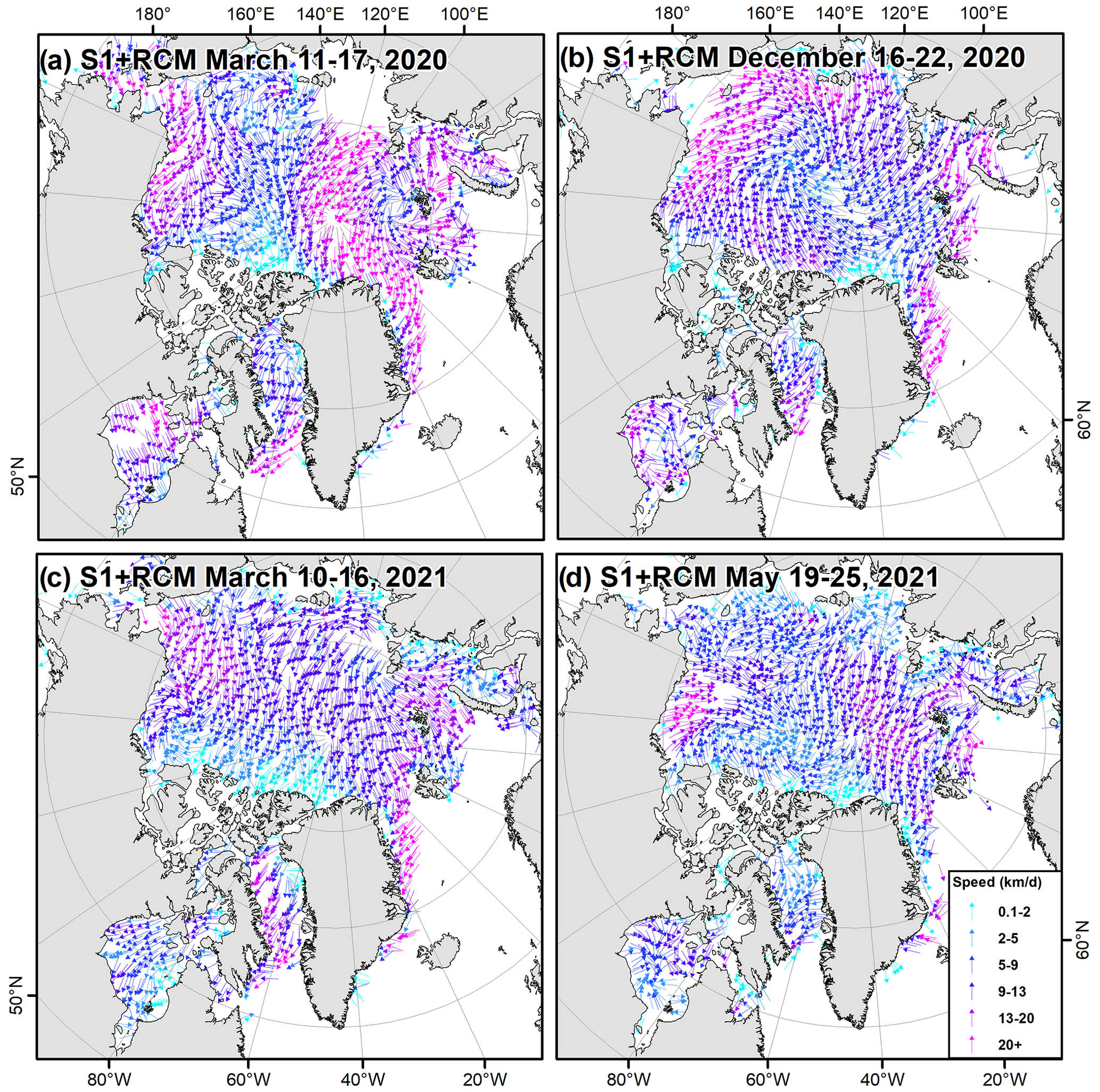
Figure 8 The spatial distribution of 25 km 7 d S1 + RCM sea ice motion on (a) 11–17 March 2020, (b) 16–22 December 2020, (c) 10–16 March 2021, and (d) 19–25 May 2021. Note that the white areas in the figure indicate either zero ice motion for the landfast ice or no ice motion information extracted (because of no SAR data, no ice, or no stable ice features).

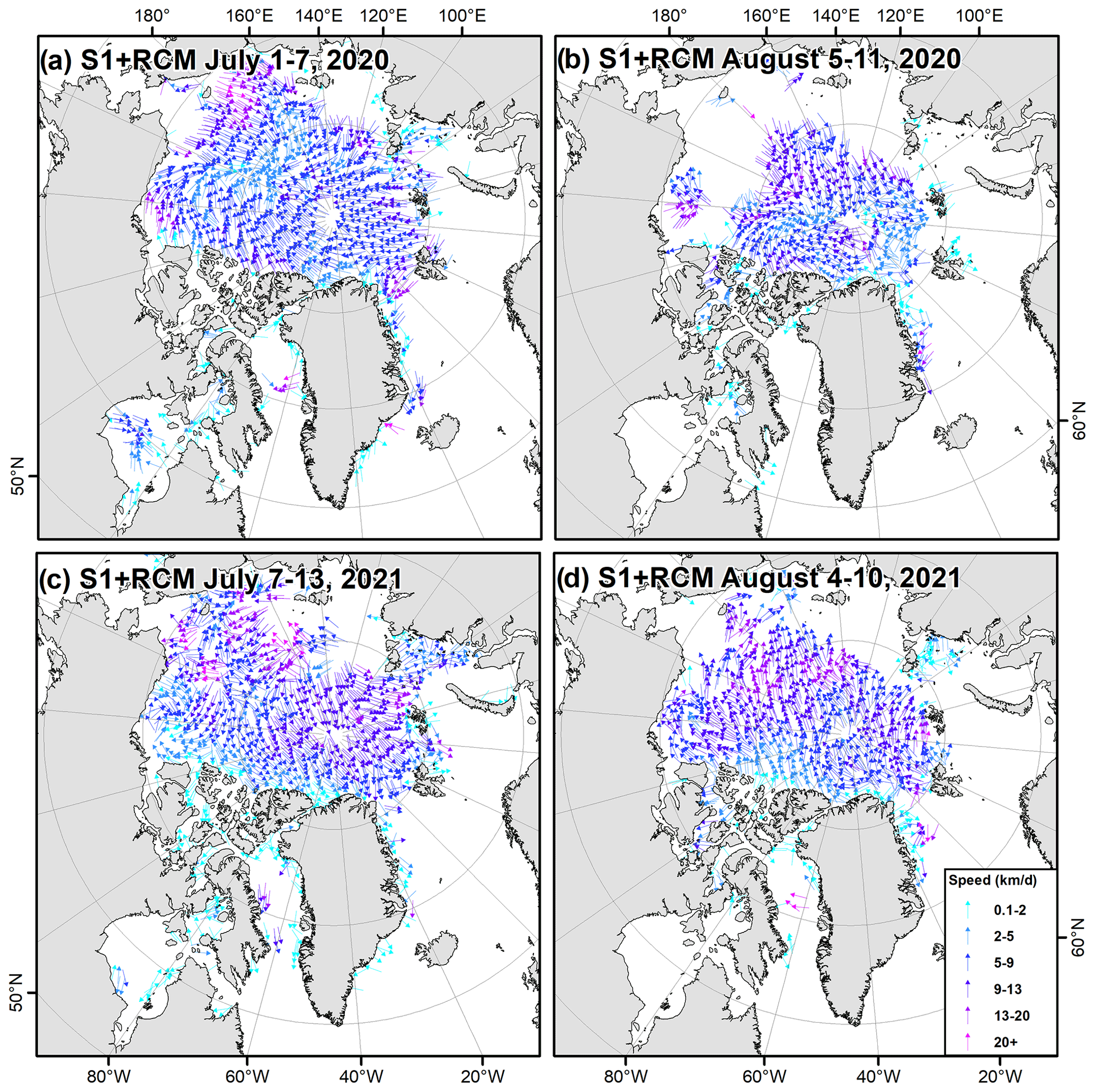
Figure 9 The spatial distribution of 25 km 7 d S1 + RCM sea ice motion on (a) 1–7 July 2020, (b) 5–11 August 2020, (c) 7–13 July 2021, and (d) 4–10 August 2021. Note that the white areas in the figure indicate either zero ice motion for the landfast ice or no ice motion information extracted (because of no SAR data, no ice, or no stable ice features).

4 Large-scale SIM from S1 + RCM

The 7 d 25 km spatiotemporal scale is able to provide the most complete picture of SIM across the pan-Arctic from SAR imagery alone; this has long been desired. Examples of 7 d 25 km S1 + RCM SIM over the pan-Arctic for selected weeks during winter months are shown in Fig. 8. Notable features include the Transpolar Drift (Fig. 8a and c), Beaufort Gyre (Fig. 8b), a Beaufort Gyre reversal (Fig. 8a), and minimal SIM because of landfast (no ice motion) ice conditions within the majority of the CAA (Fig. 8). Some spatial gaps are present in certain weeks, particularly in the Laptev Sea (Fig. 8), and these gaps in addition to others are because of the spatial variability in weekly image density of S1 + RCM (Fig. 3). Resolving SIM during the melt season, even with high-spatial-resolution SAR imagery, is more challenging than dry winter conditions because automated feature tracking is more difficult when the ice concentration is low or water is on the ice surface (e.g., Agnew et al., 2008; Lavergne et al., 2010). Examples of the spatial distribution of 25 km 7 d S1 + RCM SIM for selected weeks and summer months are shown in Fig. 9, and indeed the spatial coverage from S1 + RCM is still considerable during the summer months.

The spatial distributions of 6.25 km 3 d pan-Arctic S1 + RCM SIM for selected periods during the winter and summer are shown in Figs. 10 and 11, respectively. The insets of both Figs. 10 and 11 illustrate the level of SIM spatial detail captured at 6.25 km. More spatial gaps across the pan-Arctic use higher spatiotemporal resolution especially during the summer months. These problems relate to the challenge of constructing a complete picture of pan-Arctic SIM every 3 d using available SAR imagery because of their different acquisition scenarios. Specifically, RCM acquisitions are more spatiotemporally distributed across the Arctic and S1 acquisitions are more intensive in certain regions (Fig. 3), and as a result, some regions can be missed on certain days. This uneven spatial imaging problem is illustrated in Fig. 12, where it is apparent SIM is captured in the Beaufort Sea, Chukchi Sea, and Hudson Bay from 12–14 March 2021 but absent from 14–16 March 2021. Also, just because SAR image pairs are available over a region does not imply automatic SIM detection will be successful particularly during the summer months. Despite this, there are still many regions across the Arctic where high spatial and temporal SIM can be resolved using S1 + RCM, but the aforementioned problems need to be taken into consideration with respect to regional time series development.

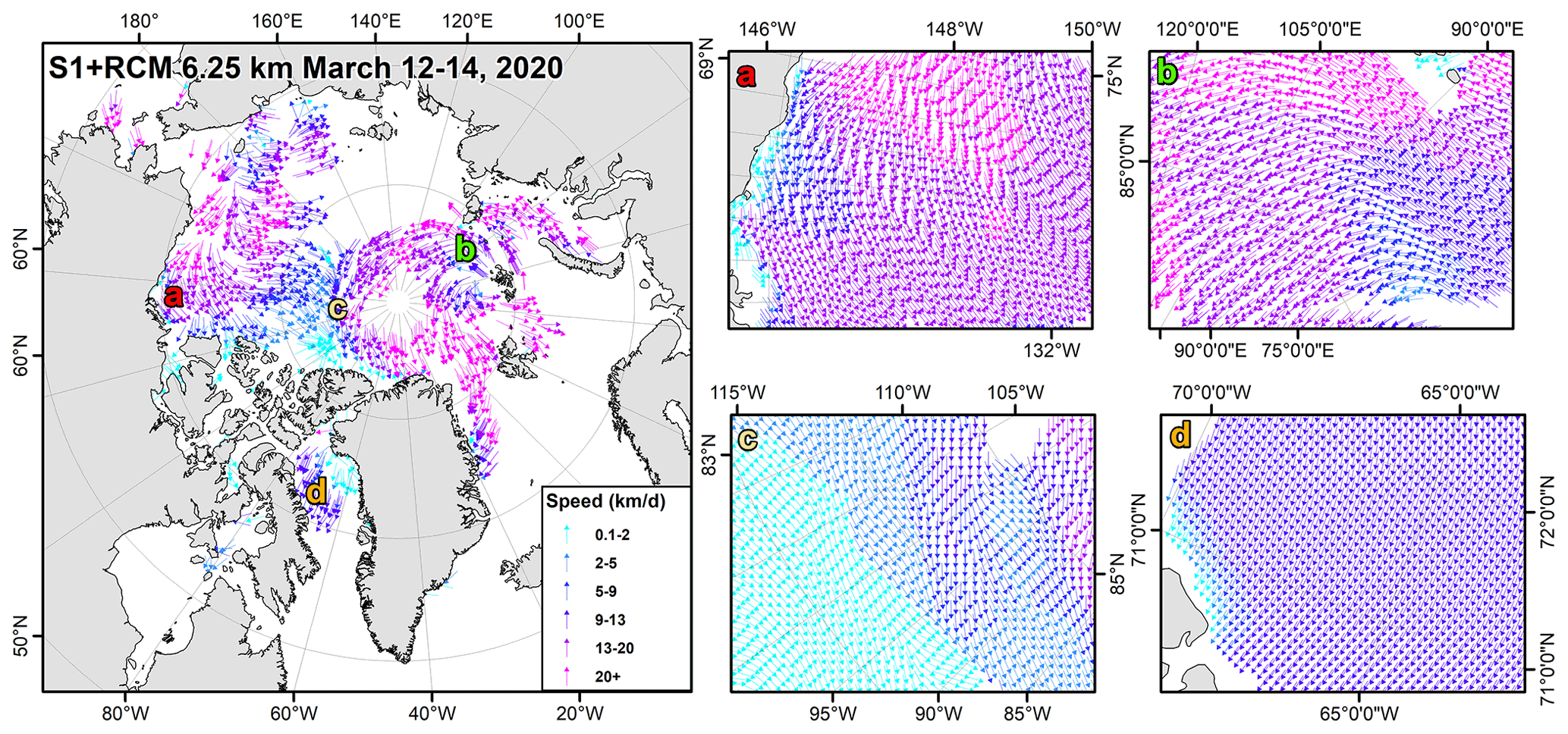
Figure 10 The spatial distribution of 6.25 km 3 d S1 + RCM sea ice motion on 12–14 March 2020. The letters correspond to zoomed-in regions on the map. Note that the white areas in the figure indicate either zero ice motion for the landfast ice or no ice motion information extracted (because of no SAR data, no ice, or no stable ice features).

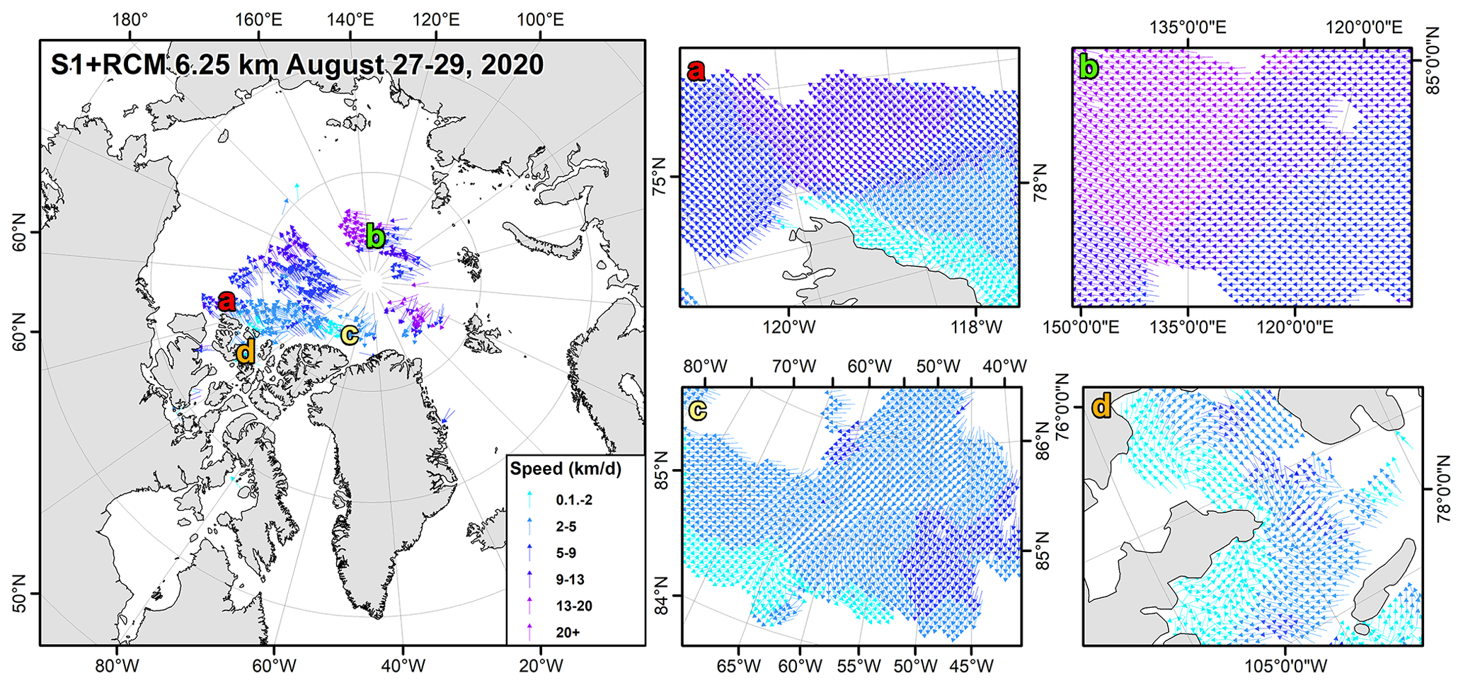
Figure 11 The spatial distribution of 6.25 km 3 d S1 + RCM sea ice motion on 27–29 August 2020. The letters correspond to zoomed-in regions on the map. Note that the white areas in the figure indicate either zero ice motion for the landfast ice or no ice motion information extracted (because of no SAR data, no ice, or no stable ice features).

Another benefit provided by S1 + RCM SIM is that SIM is resolved within the CAA, and Fig. 13. provides a more detailed look at summer SIM within the CAA. Indeed SIM in this region is very spatially heterogeneous as pointed out by Melling (2002). Estimating SIM within the CAA is challenging for coarse-resolution satellites because of its narrow channels and inlets that make automated feature tracking difficult, especially during the melt season (Agnew et al., 2008), and this is a major gap with existing SIM products. Information on SIM within the CAA is important given it contains the Northwest Passage and has experienced increases in shipping activity (e.g., Dawson et al., 2018). Both large-scale S1 + RCM SIM products generated by ECCC-ASITS provide valuable SIM information in this region not just for scientific analysis, but also for stakeholders operating in the CAA. Continued monitoring of SIM within the CAA is important as climate warming is expected make the region more navigable in the future (Mudryk et al., 2021).

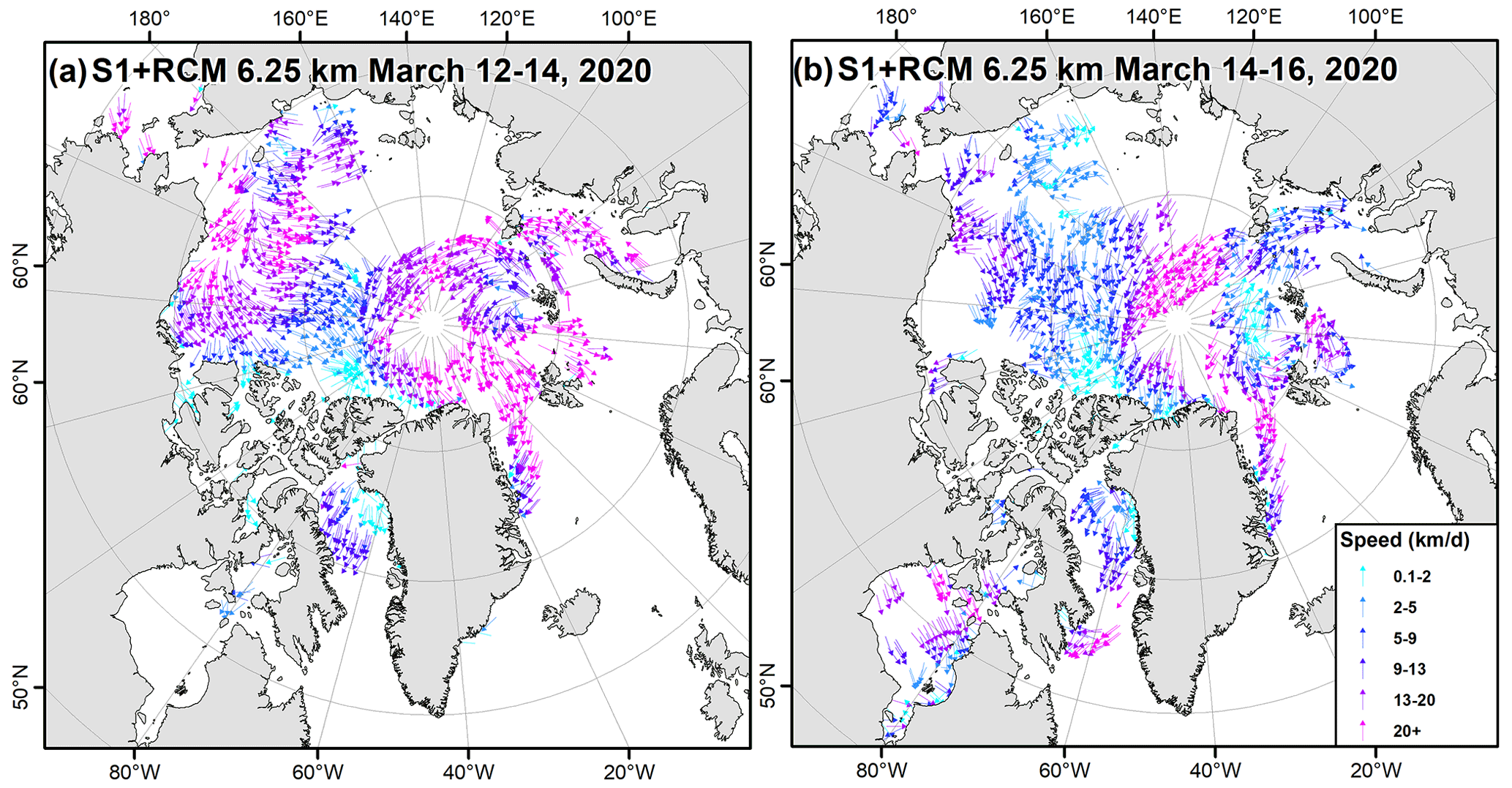
Figure 12 The spatial distribution of 6.25 km 3 d S1 + RCM sea ice motion on (a) 12–14 March 2020 and (b) 14–16 March 2020. Note that the white areas in the figure indicate either zero ice motion for the landfast ice or no ice motion information extracted (because of no SAR data, no ice, or no stable ice features).

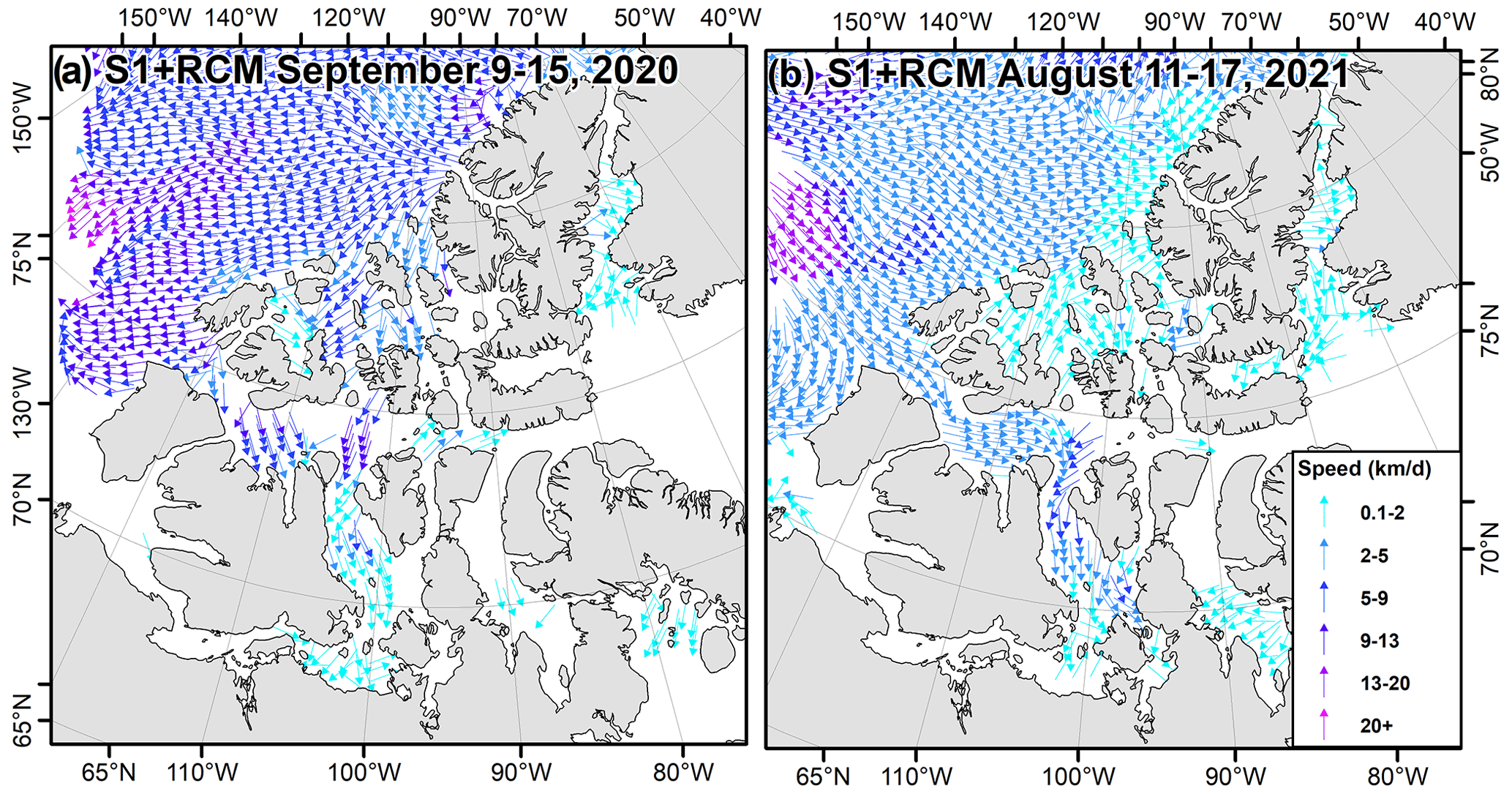
Figure 13 The spatial distribution of 25 km 7 d S1 + RCM sea ice motion surrounding the Canadian Arctic Archipelago on (a) 9–15 September 2020 and (b) 11–17 August 2021. Note that the white areas in the figure indicate either zero ice motion for the landfast ice or no ice motion information extracted (because of no SAR data, no ice, or no stable ice features).

5 S1 + RCM SIM validation and assessing uncertainty

ECCC's automated SIM tracking algorithm has previously undergone validation against buoy positions and has an uncertainty of 0.43 km derived for RADARSAT-2 SAR image pairs separated by 1–3 d (Komarov and Barber, 2014). Moreover, SIM output from the tracking algorithm has been found to be in good agreement with other tracking algorithms that include the RADARSAT Geophysical Processor System (RGPS) (e.g., Kwok, 2006; Agnew et al., 2008; Howell et al., 2013). However, considering the application of the tracking algorithm in this study represents considerably larger spatial and temporal domains, together with new satellites sensors (i.e., S1 and RCM), it is important to reassess the quality and uncertainty of the resulting S1 + RCM SIM vectors.

To provide a quality assessment of the S1 + RCM SIM vectors for each grid cell, the cross-correlation coefficients for all S1 + RCM vectors in each grid cell were averaged. Figure 14 summarizes the monthly cross-correlation coefficients of 6.25 km 3 d S1 + RCM SIM using boxplots. Note that for the ECCC automated SIM tracking algorithm, the cross-correlation coefficients are calculated for the second-order derivatives (Laplacians) of the images and not the original images; therefore, the cross-correlation coefficients may appear lower than reported in the literature by other studies. The cross-correlation coefficient exhibited the expected variability associated with the seasonal cycle of sea ice and remained relatively high and stable during the dry winter conditions (∼0.45), decreased during the melt season (∼0.33), and then returned to stability following the melt season (∼0.45). As found in previous studies, lower-quality vectors are more apparent during the shoulder seasons (i.e., melt–freeze transitions) (e.g., Agnew et al., 2008; Lavergne et al., 2010, 2021).

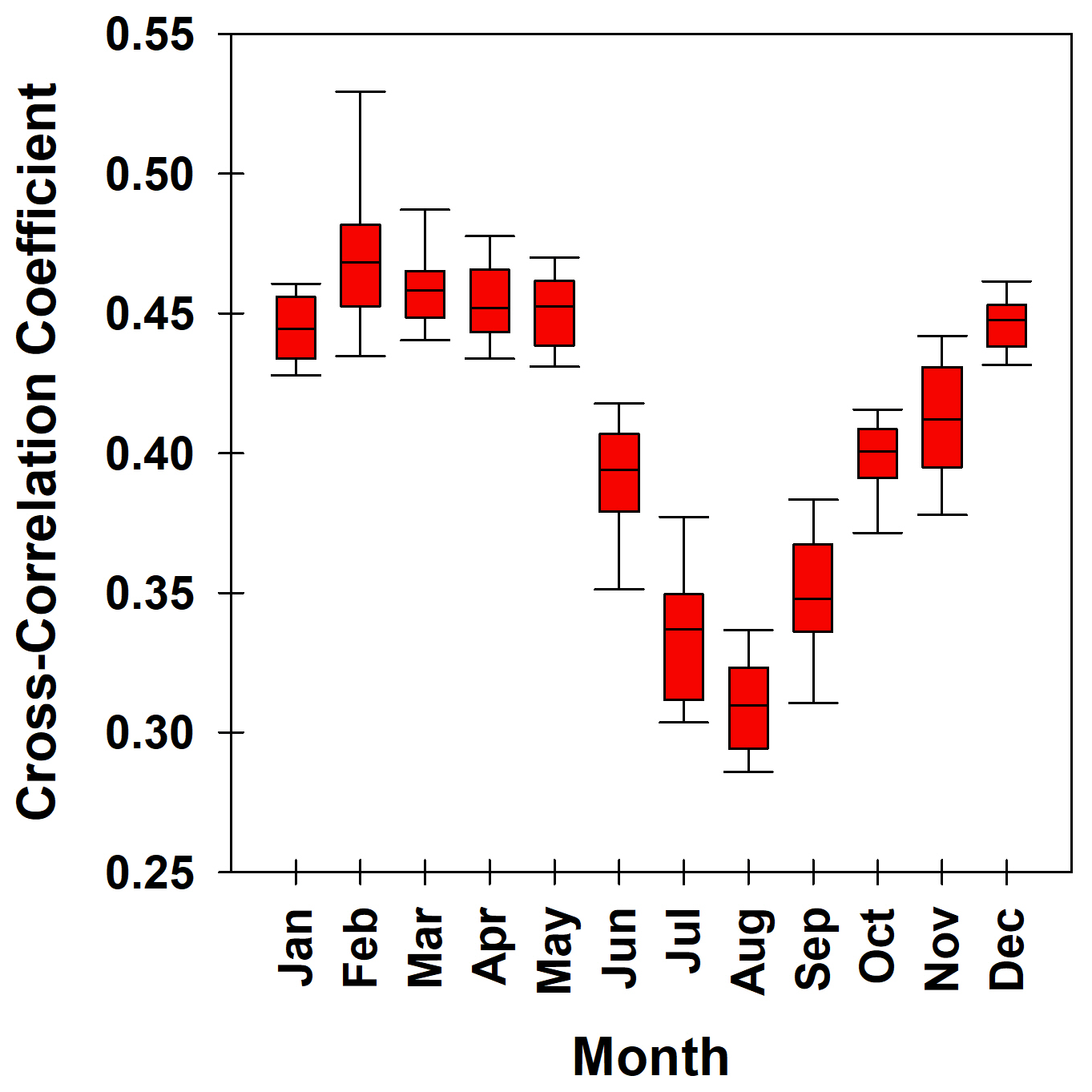
Figure 14 Boxplots of the monthly cross-correlation coefficient based on S1 + RCM SIM from March 2020 to October 2021.

In order to estimate the SIM uncertainty from the ECCC's automated SIM tracking algorithm for S1 and RCM SAR images, we compared SIM displacement vectors from S1 and RCM to buoy positions from the IABP during winter (April) and summer (August) time periods. For all S1 and RCM displacement vectors (derived from image pairs), the closest buoy trajectory was co-located to the start of each displacement vector position. The only restrictions placed on the buoys were that they were located north of 40^∘ N and the distance between the starting point of a given SAR ice motion tracking vector and the starting point of the corresponding buoy trajectory did not exceed 3 km. Figure 15 summarizes the results for dry winter conditions (April 2020 and 2021) and during the melt season (August 2020 and 2021). The ECCC automated SIM tracking algorithm performs very well during winter conditions with a root-mean-square error (RMSE) of 2.78 km and a mean difference (MD) of 0.40 km. Performance slightly decreases during the summer with a lower number of vectors detected and an RMSE of 3.43 km.

Our RMSE is higher than the value reported by Komarov and Barber (2014) likely because the initial validation assessment of the automated tracking algorithm only used 35 sample points in the Beaufort Sea during the winter and the vectors were at a higher spatial resolution (i.e., 100 m). Our RMSE is slightly higher than reported by Lindsay and Stern (2003), who compared the RGPS SIM to buoys in the Central Arctic and reported an RMSE of ∼1 km for the winter and ∼2 km for the summer. However, our RMSE estimates are much lower than Wilson et al. (2001), who compared RADARSAT-1 SAR estimates of SIM to buoys in Baffin Bay and reported an RMSE of 3.8 km for the winter and 6.8 km for the summer. The differences in RMSEs can be attributed to numerous factors including the geolocation errors of the different SAR satellites, differences in the methodology for buoy comparison, and different tracking algorithms. Overall, our validation is certainly representative of large-scale SIM uncertainty because we considered a wide range of ice conditions during both the winter and summer months.

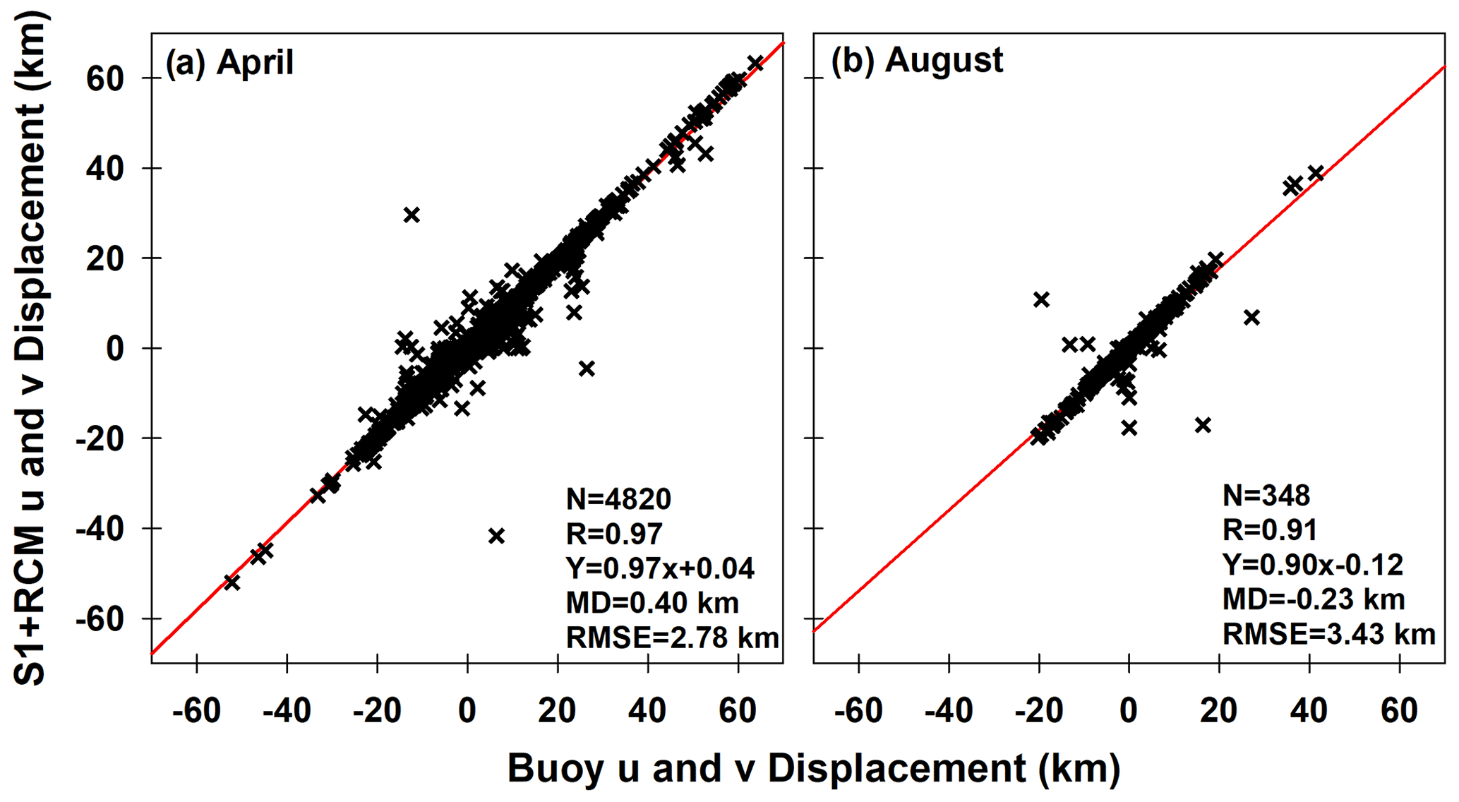
Figure 15 Comparison between ice motion vectors derived by the Komarov and Barber (2014) automated sea ice tracking algorithm from S1 and RCM SAR images and buoy data.

Taking into consideration the difference between the winter and the summer, we assign two uncertainties to the S1 + RCM SIM products for dry and wet conditions as follows. Consider a grid cell containing a set of N sea ice velocity vectors V_i, where $i=\mathrm{1},\mathrm{2},\mathrm{\dots },N$. Ice speed for this each vector has the following uncertainty associated with the SIM tracking algorithm deriving the ice motion vector from two consecutive images:

$$\begin{array}{}\text{(1)}& \mathrm{\Delta }{V}_i={\displaystyle \frac{s_o}{\mathrm{\Delta }{t}_i}},\end{array}$$

where Δt_i is the time interval (in days) separating two SAR images used to derive the considered ice velocity vector V_i. In Eq. (1) s_o is the uncertainty in sea ice displacement (not speed) for dry ice conditions (2.78 km) or wet ice conditions (3.43 km). Note that s_o must be divided by Δt_i to come up with the ice velocity uncertainty. The average uncertainty for dry (s_o=2.78 km) and wet (s_o=3.43 km) ice conditions in each grid cell (N) is then determined using the following equation:

$$\begin{array}{}\text{(2)}& {\mathit{\sigma }}_{\mathrm{SIM}}={\displaystyle \frac{\mathrm{1}}{N}}\sum _{i=\mathrm{1}}^N\mathrm{\Delta }{V}_i.\end{array}$$

Figure 16 shows an example of the spatial distribution of both dry and wet uncertainty estimates indicating higher uncertainty estimates for the latter. We acknowledge that it is difficult to quantify the impact of SAR image pair availability over 7 d together with automatic SIM vector detection under certain environmental conditions. The number of S1 + RCM SIM vectors used in the grid cell generation can subsequently be used to account for this, whereby more confidence (less uncertainty) in SIM can be associated with a larger number of vectors. Moreover, S1 + RCM image density increases with latitude (Fig. 3), indicating that more consistent coverage is available over the Central Arctic, which is also beneficial during the melt season when automated SIM tracking algorithms have more difficulty. However, SAR image pair coverage could be exceptional over the 7 d time window, yet environmental conditions (i.e., melt ponds, low ice concentration, marginal ice zone, etc.) could still make automatic SIM vector detection difficult, resulting in a low number of SIM vectors in the grid cell. The problem of image coverage is less of a concern for the 3 d product given the average image separation is ∼2 d.

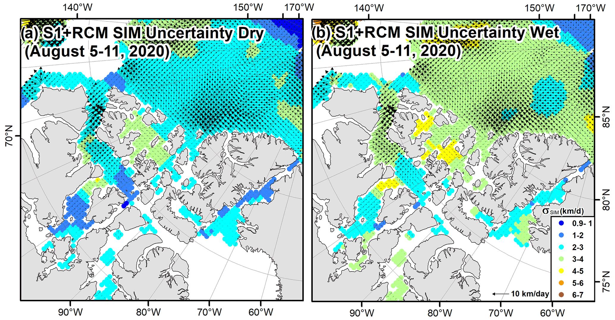
Figure 16 Spatial distribution of (a) dry and (b) wet S1 + RCM SIM uncertainty for 5–11 August 2020.

6 SIM comparison between S1 + RCM, NSIDC, and OSI SAF

Given the difficultly in quantifying SAR image pair coverage on S1 + RCM SIM uncertainty, we now compare S1 + RCM SIM to the NSIDC and OSI SAF SIM products that are widely utilized by the sea ice community. Such a comparison provides additional quantitative confidence metrics to assess the quality of the S1 + RCM SIM estimates. To facilitate a representative one-to-one grid cell comparison between S1 + RCM SIM and both the NSIDC and OSI SAF SIM products, the spatial and temporal resolution of the S1 + RCM were matched with the NSIDC and OSI SAF SIM products from March to December 2020. For OSI SAF, S1 + RCM was generated with a 2 d temporal resolution and 62.5 km spatial resolution, and for NSIDC, S1 + RCM was generated with a 7 d temporal resolution and 25 km spatial resolution. For each product's temporal resolution (i.e., 7 d for NSIDC and 2 d for OSI SAF), all the S1 + RCM SIM vectors within each product's grid cells (i.e., 25 km for NSIDC and 62.5 km for OSI SAF) were averaged. This resulted in 455 905 grid cells for the S1 + RCM and NSIDC comparison and 376 386 grid cells for the S1 + RCM and OSI SAF comparison. More samples were available from NSIDC because of its higher spatial resolution.

Scatterplots of the u and v vector components of SIM for S1 + RCM versus NSIDC and OSI SAF are shown in Figs. 17 and 18, respectively. Both existing SIM products are in good agreement with S1 + RCM, with correlation coefficients for u and v of 0.75 and 0.78, respectively, for the NSIDC and 0.84 and 0.85, respectively, for OSI SAF providing confidence in the SAR coverage for the 7 d and 3 d S1 + RCM products. The RMSE is higher for the NSIDC (u=4.6 km d⁻¹ and v=4.7 km d⁻¹) compared to OSI SAF (u=3.9 km d⁻¹ and v=3.9 km d⁻¹), and we note the better agreement between S1 + RCM and OSI SAF is likely because the temporal resolution more closely matches the average overlap between SAR images (i.e., ∼2 d). However, the overall higher speed associated with S1 + RCM is most likely the result of higher spatial resolution compared to lower-resolution satellite data used in NSIDC and OSI SAF as faster speeds are more difficult to track at lower spatial resolution because of temporal decorrelation. Kwok et al. (1998) also noted this problem when comparing SIM from passive microwave with SAR and found it also applies to regions of low ice concentration. Figures 17 and 18 also illustrate that users of either the NSIDC or OSI SAF SIM products are underestimating SIM.

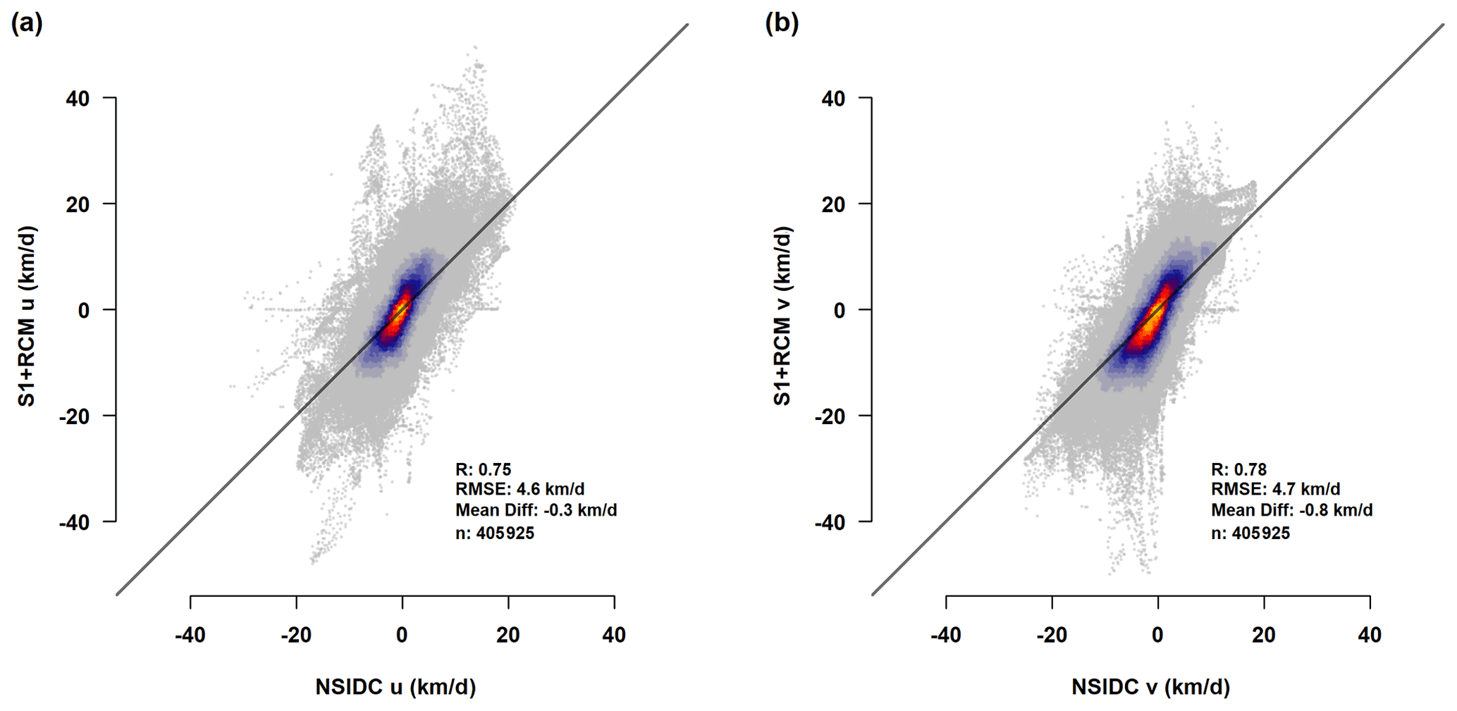
Figure 17 Heat scatterplots of S1 + RCM sea ice motion versus National Snow and Ice Data Center (NSIDC) SIM for (a) u and (b) v vector components. Also shown is the number of samples (n), Pearson's correlation coefficient (R), root-mean-square error (RMSE), and the mean difference (MD).

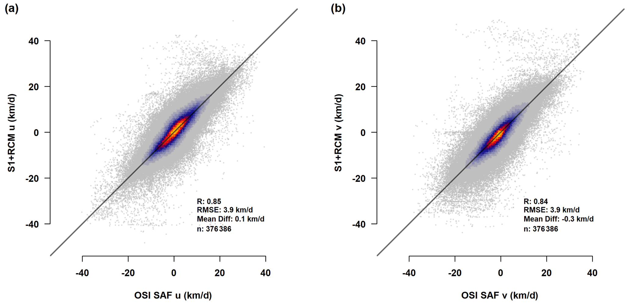
Figure 18 Heat scatterplots of S1 + RCM sea ice motion versus Ocean and Sea Ice Satellite Application Facility (OSI SAF) SIM for (a) u and (b) v vector components. Also shown is the number of samples (n), Pearson's correlation coefficient (R), root-mean-square error (RMSE), and the mean difference (MD).

7 Conclusions

In this study, we described the ECCC-ASITS and its application of 135 471 images from five SAR satellites from S1 and the RCM to routinely estimate SIM over the large-scale pan-Arctic domain from March 2020 to October 2021. The higher-density image coverage of S1 + RCM as opposed to just S1 and/or RCM provided more available SAR image pairs over the Hudson Bay, Davis Strait, Beaufort Sea, Bering Sea, and the North Pole. S1 + RCM SIM covered the majority of the pan-Arctic domain using a spatial resolution of 25 km and temporal resolution of 7 d. The 6.25 km 3 d products also were generated and can provide improved spatiotemporal SIM representation in many regions of the pan-Arctic. In particular, the spatial heterogeneity in large-scale S1 + RCM SIM at both scales was preserved, and SIM was able to be resolved within the narrow channels and inlets of the CAA, filling a major information gap.

The S1 + RCM SIM vectors were compared against buoy estimates from the IABP for both dry and wet ice conditions to assess the performance of the ECCC automated feature tracking algorithm with S1 and RCM imagery. Results indicate an uncertainty of 2.78 km for the former and 3.43 km for the latter, and we developed a range of ice speed uncertainties for the S1 + RCM SIM products. Comparing the S1 + RCM SIM estimates to the existing SIM datasets of NSIDC and OSI SAF revealed that S1 + RCM provides larger ice speeds (∼4 km d⁻¹) confirming the speed bias associated with lower-resolution sensors.

The primary purpose of ECCC-ASITS is to routinely deliver SIM information for operational usage within ECCC as well as the scientific community and maritime stakeholders. The data archive is available from March 2020 to October 2021, and updates are produced ad hoc (every few months), but updates are expected to occur more frequently in the near future. We recognize that the short data record of S1 + RCM SIM does not make it well suited for long-term scientific studies. However, the Arctic sea ice is rapidly changing, and for recent large-scale process studies or localized studies (e.g., MOSAiC) or regional studies (e.g., CAA) S1 + RCM SIM products generated by the ECCC-ASITS can provide more representative SIM estimates than their passive microwave counterparts. Moreover, the time series of large-scale generated SIM from SAR needs to start now with the currently available and expected continuation of spaceborne SAR missions. The anticipated launch of the NASA-ISRO (NISAR) L- and S-band SAR satellite also provides an opportunity to add L-band into the ECCC-ASITS. L-band SAR would be able to provide improved SIM estimates during the melt season compared to C-band (Howell et al., 2018). Even without adding different frequency satellite sensors, the upcoming launch of Sentinel-1C and Sentinel-1D will continue to facilitate the routine generation of large-scale SIM using the ECCC-ASITS from C-band SAR for many years to come.

Future refinements to the ECCC-ASITS are possible, which includes adding the HV channel to complement SIM estimated from HH polarization. Mixing S1 and RCM images offers an opportunity to provide more spatiotemporally refined SIM estimation across the Arctic; however, based on the current image distribution of S1 and RCM, it is unlikely to improve spatial coverage as RCM mainly fills in the spatial gaps in S1 coverage. It is also very challenging computationally to produce and work with large-scale SAR-derived SIM products at very high spatiotemporal resolution. To that end, mixing sensors at C-band will likely not result in major advances of large-scale automated detected SIM, but it could provide more insight into local-scale processes (e.g., fault generation, instantaneous reaction to forcing, inertial oscillations to name a few). In this regard, the temporal resolution of mixing S1 and RCM imagery could be pushed to sub-daily in some regions, and we anticipate exploring this option for targeted dense time series applications in the Arctic. While groups such as the Polar Space Task Group aim to improve or refine SAR coverage across the pan-Arctic over the annual cycle, it is unlikely a purely SAR derived SIM product will be able to achieve daily or sub-daily coverage consistently across the pan-Arctic. This has only recently been achieved with passive microwave observations using a swath-to-swath approach (Lavergne et al., 2021). Therefore, it could be worth exploring the complement of SIM provided from passive microwave swath to swath and SIM generated from SAR.