the Creative Commons Attribution 4.0 License.
the Creative Commons Attribution 4.0 License.
 | 13 Dec 2021
Improving surface melt estimation over the Antarctic Ice Sheet using deep learning: a proof of concept over the Larsen Ice Shelf
Peter Kuipers Munneke
Stef Lhermitte
Maaike Izeboud
Michiel van den Broeke
Accurately estimating the surface melt volume of the Antarctic Ice Sheet is challenging and has hitherto relied on climate modeling or observations from satellite remote sensing. Each of these methods has its limitations, especially in regions with high surface melt. This study aims to demonstrate the potential of improving surface melt simulations with a regional climate model by deploying a deep learning model. A deep-learning-based framework has been developed to correct surface melt from the regional atmospheric climate model version 2.3p2 (RACMO2), using meteorological observations from automatic weather stations (AWSs) and surface albedo from satellite imagery. The framework includes three steps: (1) training a deep multilayer perceptron (MLP) model using AWS observations, (2) correcting Moderate Resolution Imaging Spectroradiometer (MODIS) albedo observations, and (3) using these two to correct the RACMO2 surface melt simulations. Using observations from three AWSs at the Larsen B and C ice shelves, Antarctica, cross-validation shows a high accuracy (root-mean-square error of 0.95 mm w.e. d−1, mean absolute error of 0.42 mm w.e. d−1, and a coefficient of determination of 0.95). Moreover, the deep MLP model outperforms conventional machine learning models and a shallow MLP model. When applying the trained deep MLP model over the entire Larsen Ice Shelf, the resulting corrected RACMO2 surface melt shows a better correlation with the AWS observations for two out of three AWSs. However, for one location (AWS 18), the deep MLP model does not show improved agreement with AWS observations; this is likely because surface melt is largely driven by factors (e.g., air temperature, topography, katabatic wind) other than albedo within the corresponding coarse-resolution model pixels. Our study demonstrates the opportunity to improve surface melt simulations using deep learning combined with satellite albedo observations. However, more work is required to refine the method, especially for complicated and heterogeneous terrains.
- Article
(12678 KB) - Full-text XML
- BibTeX
- EndNote


The Antarctic Ice Sheet (AIS) is an important indicator of climate change. Current AIS mass loss has been estimated at 155±19 Gt yr−1 (0.43±0.05 mm yr−1 of eustatic sea level rise) between 2006 and 2015 and is accelerating (Pörtner et al., 2019). At present, mass loss is mainly driven by ice shelf weakening due to basal melt (The IMBIE team, 2018) or damage processes (Lhermitte et al., 2020) or by hydrofracturing due to surface melt (The IMBIE team, 2018; Gilbert and Kittel, 2021; Kuipers Munneke et al., 2014). In the coming centuries, surface melt is projected to increase strongly over Antarctica (Trusel et al., 2015), increasing the incidence of surface-melt-related instability of ice shelves. The Intergovernmental Panel on Climate Change (IPCC) estimated the contribution from AIS mass loss to global mean sea level rise until 2100 in its recent Sixth Assessment Report (IPCC AR6; Fox-Kemper et al., 2021). Under different Shared Socioeconomic Pathway (SSP) scenarios, the contribution will likely be 0.03–0.27 m (SSP1–2.6), 0.03–0.29 m (SSP2–4.5), or 0.03–0.34 m (SSP5–8.5) (Fox-Kemper et al., 2021). In this context, accurate information about surface melt can directly enhance our understanding of the AIS evolution and its contribution to sea level rise.
Despite the importance of melt volumes estimates, deriving them accurately from satellite observations or (regional) climate models is not straightforward. Satellite estimates rely, for example, on proxies of melt presence from changes in albedo (Steffen et al., 1993; Pirazzini, 2004), brightness temperature (Zheng et al., 2020, 2019), or backscatter (Trusel et al., 2013, 2012) to empirically estimate melt flux or melt volumes. However, these satellite methods face difficulties as they often require locally adapted thresholds (e.g., thresholds in Trusel et al., 2013) or potentially underestimate the melt fluxes over, for example, blue ice areas (Arthur et al., 2020; Lenaerts et al., 2017), where the contrast between melt and no-melt is less clear.
Climate models, including regional climate models, on the other hand, face difficulties in accurately estimating surface melt over areas with low surface albedo. Often, features of strong surface melt (ponds, blue ice, lakes) are smaller than the model resolution, and processes that lead to their appearance and dynamics are usually not well represented (Lenaerts et al., 2017; Kingslake et al., 2017). Optical remote sensing provides high-quality albedo observations at different spatiotemporal resolutions; hence, it is a competent additional source of data to the albedo simulation from a physically based climate model. Therefore, we propose a deep learning method that uses the albedo observations from remote sensing to correct for the shortcomings of climate models. Deep learning is a machine learning technique that extracts multiple levels of abstraction/representation of data based on multiple processing layers, i.e., artificial neural networks (LeCun et al., 2015). To date, deep learning has been widely applied in Earth system science to analyze and correct mismatches between model simulations and observations (Reichstein et al., 2019); an important reason for this is that deep learning models execute much faster than physically based models.
Our study aims to develop a novel framework correcting the model–observation mismatch of surface melt in the AIS with a deep learning model that utilizes inputs from the physically based model, the regional atmospheric climate model version 2.3p2 (RACMO2), and remote sensing albedo observations from the Moderate Resolution Imaging Spectroradiometer (MODIS). To achieve this, our study has two primary objectives: (1) develop a deep learning model to correct the simulations of surface melt from RACMO2 based on automatic weather station (AWS) observations, and (2) apply and evaluate the performance of the developed model in correcting the surface melt simulations from RACMO2. To prove the concept of this framework, we apply it to RACMO2 model simulations over the Larsen Ice Shelf between 2009 and 2016, using meteorological parameters from RACMO2 and remote sensing observations of surface albedo. In Sect. 2, we introduce the investigated area and specify all data sets. The architecture of the method and its details are described in Sect. 3. Sections 4 and 5 present and discuss the results, followed by a summary in Sect. 6.
2.1 Study area
We apply the deep learning framework to the Larsen Ice Shelf, situated to the east of the Antarctic Peninsula. According to existing estimates, this area produces about 50 % to 60 % of all surface meltwater in Antarctica (Kuipers Munneke et al., 2012a; Trusel et al., 2013). On average, surface melt occurs on 25 d yr−1 in the southern part of Larsen C Ice Shelf and on over 75 d yr−1 in the western and northern parts of the region (Luckman et al., 2014). The Larsen Ice shelf is an ideal test location for developing a framework to improve surface melt estimates because (1) there is abundant melt, (2) high-quality multiyear AWS data suitable for melt calculations (i.e., including the surface radiation budget) are available (Jakobs et al., 2020a), and (3) a previous comparison between RACMO2 albedo and radar backscatter from the Quick Scatterometer (QuikSCAT) revealed that both positive and negative values of the difference between RACMO2 and observed surface melt exist in this area (Trusel et al., 2013). Thus, the versatility of the method is tested both for enhancing and reducing surface melt.
The Antarctic Peninsula (Fig. 1) is the mildest region of Antarctica, as it protrudes farther north than other regions, into the Southern Ocean. In the western part of the Antarctic Peninsula, the atmospheric circulation is northwest–southeast, leading to mild conditions, few ice shelves, and little sea ice. Conversely, in the eastern Antarctic Peninsula, the circulation is south–north, resulting in colder conditions, extensive ice shelves, and year-round sea ice cover. Therefore, ice shelves on the Antarctic Peninsula are mostly located on the eastern coast. Under specific conditions, westerly atmospheric flow leads to warm and dry winds, known as föhn, descending from the eastern mountain flanks onto the ice shelves (Elvidge and Renfrew, 2016; Datta et al., 2019). These föhn winds are known to generate strong surface melt in the inlets on the ice shelves just downslope of the mountains. On average, the annual melt exceeds 400 mm w.e. (Trusel et al., 2013; Turton et al., 2020) in these inlets, distributed over about 100 melt days (Luckman et al., 2014). However, further east on the Antarctic Peninsula ice shelves, surface melt rates are also high compared with most other ice shelves in Antarctica, at 200 to 300 mm w.e. yr−1 (Trusel et al., 2013).
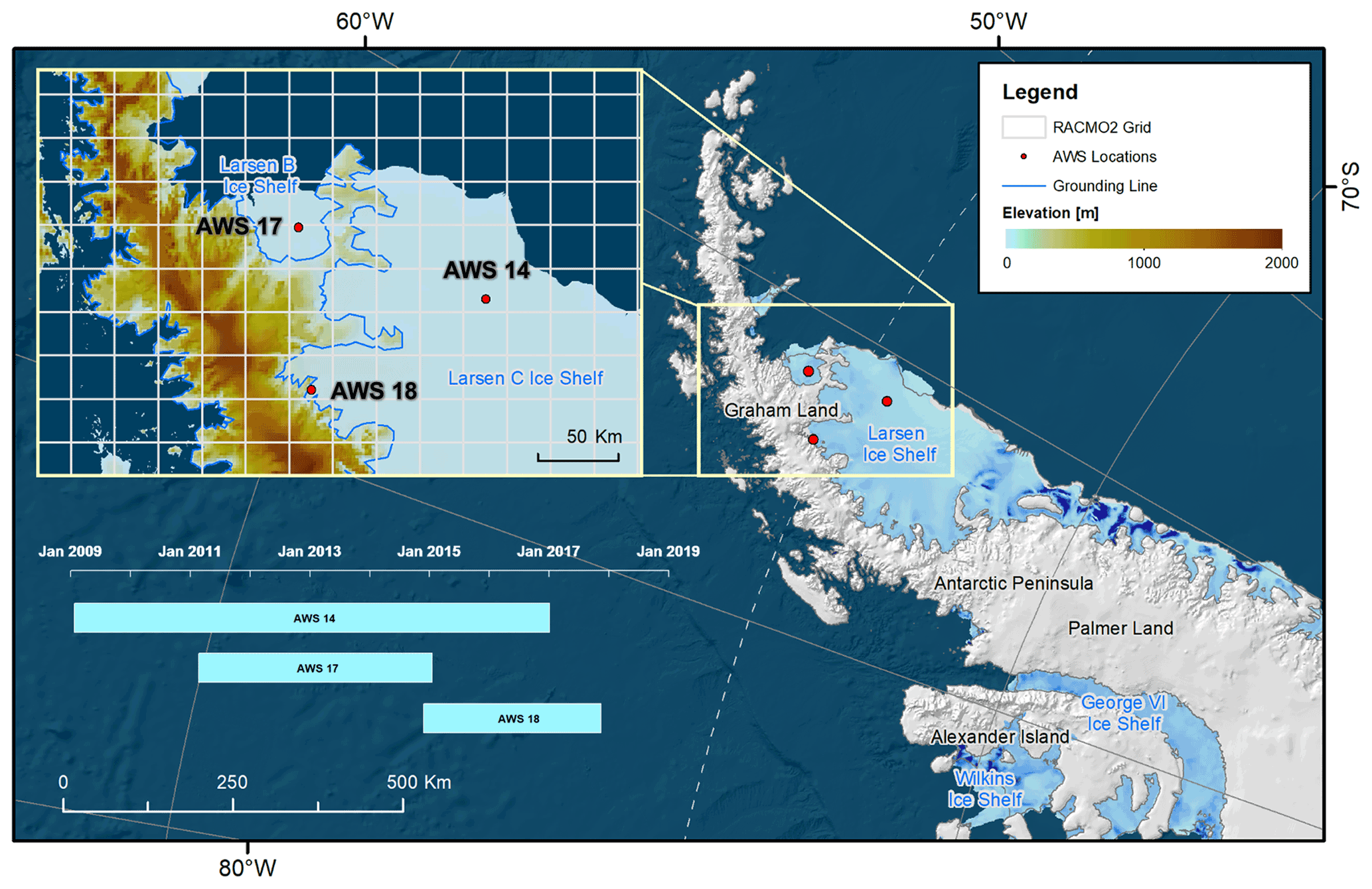
Figure 1Overview of the study area, the Larsen Ice Shelf, and details about the geolocations and operation periods of the deployed automatic weather station (AWS) observations. Surface elevation is derived from the ETOPO1 1 Arc-Minute Global Relief Model (https://www.ncei.noaa.gov/access/metadata/landing-page/bin/iso?id=gov.noaa.ngdc.mgg.dem:316, last access: 3 December 2021), and the grounding line information is derived from Bindschadler et al. (2011). The base maps are the Moderate Resolution Imaging Spectroradiometer (MODIS) Image Mosaic and the Antarctic ice-shelf buttressing (Fürst et al., 2016).
2.2 Data
2.2.1 Satellite observations
MODIS aboard the Terra (launched in 1999) and Aqua (launched in 2002) satellites provides continuous observation of the Earth's surface. For various disciplines, there are different standard MODIS data products for global change studies. Among these products, we deployed the bihemispherical reflectance (i.e., white-sky albedo) for shortwave broadband from the MCD43A3 albedo product (Schaaf and Wang, 2015) archived in the Google Earth Engine (GEE; Gorelick et al., 2017) as the albedo input. Furthermore, to obtain observational information about cloud coverage at AWS locations, cloud classifications are taken from the MOD09GA daily surface reflectance product (i.e., “MODIS/Terra Surface Reflectance Daily L2G Global 1 km and 500 m SIN Grid”; Vermote and Wolfe, 2015), also archived in GEE. To confirm the spatiotemporal melt pattern in the study area, we derived the backscattering coefficient drops as an indicator of surface melt, following Luckman et al. (2014) and Datta et al. (2019), from some representative Sentinel-1 imagery archived in GEE between January and March in 2015.
2.2.2 Automatic weather station (AWS) observations
AWS 14, AWS 17, and AWS 18 (Fig. 1) are automatic weather stations installed and operated by the Institute for Marine and Atmospheric research Utrecht (IMAU) and the British Antarctic Survey (BAS). Incoming and reflected shortwave radiation (S↓ and S↑, respectively) and surface albedo (αo) are observed using a Kipp & Zonen CNR 1 radiation sensor at AWS 14 and AWS 17 and using a CNR 4 radiation sensor at AWS 18. The same sensor also measures down- and upwelling longwave radiation (Rl). Air temperature (T2 m), air pressure (p), and relative humidity (RH) measured at 1–4 m above the surface are corrected for heating of the shielded housing by solar radiation, especially in situations with low wind speed. More details on the experimental setup and data corrections can be found in Kuipers Munneke et al. (2018b), Smeets et al. (2018), and Jakobs et al. (2020a).
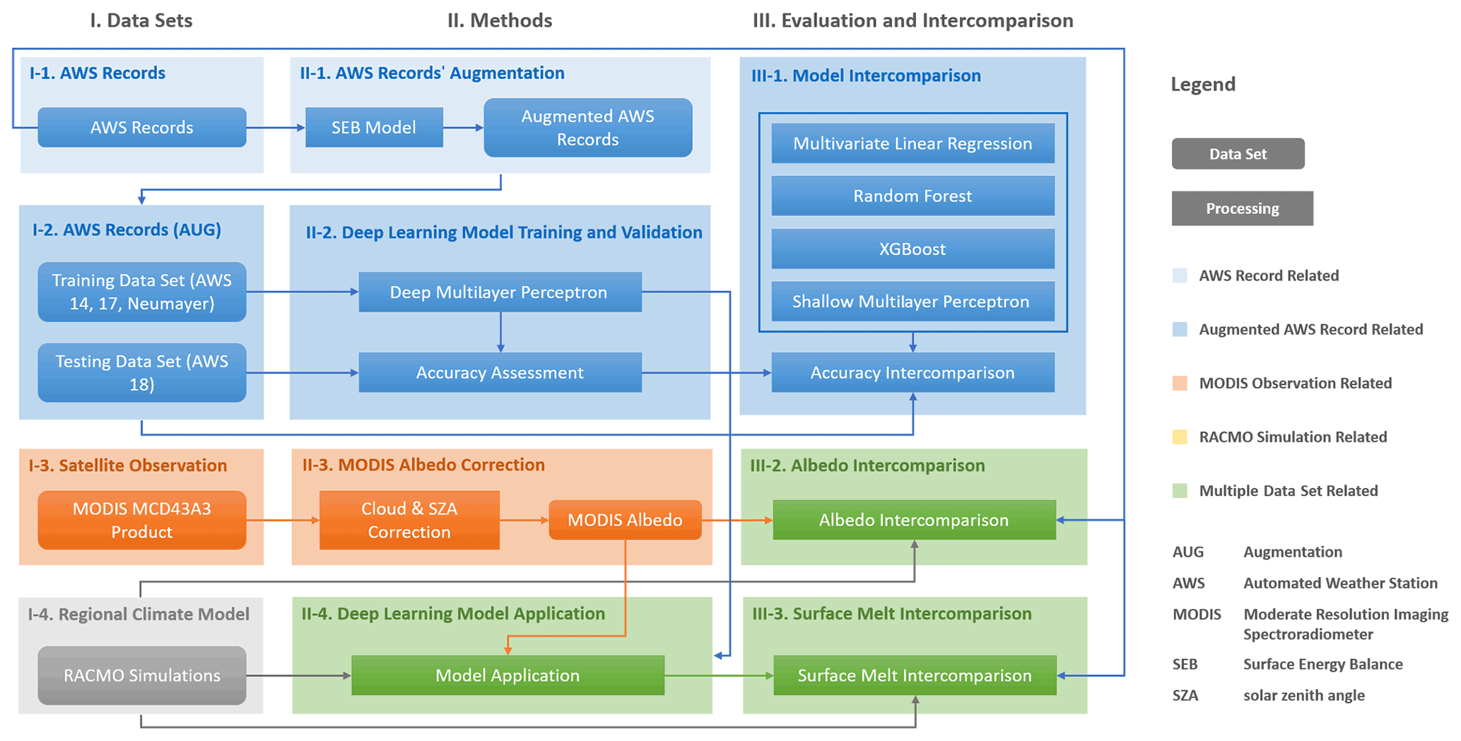
Figure 2Overall flowchart illustrating the employed data sets, implemented methods, and corresponding intercomparisons and evaluations.
2.2.3 The regional climate model RACMO2
RACMO2 is a regional climate model adapted for the simulation of the weather over snow and ice surfaces, in order to obtain a more accurate representation of surface mass and energy balance. The version used in this study is RACMO 2.3p2 forced by ERA-Interim (van Wessem et al., 2018). The entire AIS is simulated at a horizontal resolution of approximately 27×27 km2 for the period from 1979 to 2019. For this study, we select the model output between 2009 and 2016, overlapping with the availability of MODIS and AWS observations on the Larsen Ice Shelf. RACMO2 has a scheme for calculating the evolution of snow albedo, which is a key parameter for the surface energy balance in summer and an important factor in determining surface melt. The albedo scheme is based on the metamorphism of snow grains determining the amount of incoming radiation that is absorbed in the snowpack. The albedo scheme does not account for ponding meltwater, the appearance of blue ice, or other icy surfaces like wind glaze or refrozen supraglacial water. All of these surface types tend to have a lower albedo than a snow surface (Kuipers Munneke et al., 2011).
Essentially, we develop a deep learning model that corrects RACMO2 surface melt, based on differences in modeled and observed surface albedo values. A comprehensive flowchart of the method is given in Fig. 2. Input to the deep learning model consists of relevant, predictive meteorological input and the difference between observed and simulated albedo values (Δα). The deep learning model needs to be trained (Fig. 2, panel II-2), which is performed on a reference data set derived from AWS observations. To build this reference data set, the surface energy balance model is used to perturb the surface albedo from AWS observations by an amount Δα (Fig. 2, panel II-1). The model is then trained to predict the resulting change in surface melt. The trained model is subsequently applied to RACMO2, where Δα is computed as the difference between MODIS-observed albedo and RACMO2-simulated albedo (Fig. 2, panel II-4). The MODIS white-sky albedo is converted to blue-sky albedo by correcting for variations in solar zenith angle and for cloud cover (Fig. 2, panel II-3) to allow for a comparison with the RACMO2 blue-sky albedo.
The remainder of this section describes the methodology in more detail. The perturbation of the AWS observations, as described above, is referred to as “AWS data augmentation”, a frequently used term in deep learning. More fundamentals and terminology in deep learning can be found in LeCun et al. (2015). In order, we present details of (1) the formulation of the concept of the deep learning model, (2) the surface energy balance model design, (3) the augmentation (perturbation) of AWS observations, (4) training and validation of the deep learning model, (5) preparation and correction of MODIS albedo, and (6) the final application of the deep learning model as well as its evaluation (Fig. 2).
3.1 Formulation of the concept of this study
Previously, the additional absorbed solar energy that stems from the difference between a lower observed albedo and a higher modeled albedo has been converted entirely to surface melt (Lenaerts et al., 2017). However, this approach neglects the fact that all of the terms in the surface energy balance change when surface albedo is lowered; for example, it could lead to a higher surface temperature and, thus, enhanced heat loss by longwave radiation to the atmosphere, or a decreased air temperature gradient in the atmospheric boundary layer could diminish the amount of sensible heat added to the surface by turbulence. Therefore, our approach makes use of (1) original, imperfect model albedo; (2) MODIS albedo observations; and (3) a full surface energy balance model to compute the effect of a change in surface albedo on all energy balance terms.
Central to our approach, we assume that an imperfect RACMO2 simulation of surface melt is caused by an imperfect simulation of surface albedo in the model. Absorbed solar radiation is by far the major source of energy for surface melt in the summertime surface energy balance of the Antarctic surface (Lenaerts et al., 2017). Surface albedo strongly modulates this amount of absorbed solar radiation. Therefore, we assume that an imperfect simulation of surface albedo is the most dominant cause of mismatches between modeled and observed surface melt (Lenaerts et al., 2017).
3.2 Surface energy balance model
The surface energy balance is given as
Here, the radiative fluxes are represented by S↓ and S↑ (incoming and reflected solar radiation, respectively) and by L↓ and L↑ (downwelling and upwelling longwave radiation, respectively). H and L are the respective turbulent fluxes of sensible and latent heat, and G is the ground heat flux at the snow surface, computed from subsurface temperature. The sum of these fluxes is zero if the surface temperature is below the freezing point. At the freezing point, the sum of the fluxes equals the melt energy M0. All fluxes are defined positive towards the surface and are expressed in watts per square meter (W m−2). The model is identical to the one described in Kuipers Munneke et al. (2012b). The model settings (mainly for turbulent exchange of energy) were calibrated by minimizing the difference between observed and modeled surface temperature and subsurface temperatures.
3.3 AWS perturbation
The deep learning model needs to be trained to predict the amount by which the surface melt is changed (Ma) if albedo is changed by an amount Δα (Fig. 2, panel II-1). Therefore, we construct a reference data set by artificially raising or lowering the albedo, using the surface energy balance model to quantify how the reduced (additional) amount of absorbed solar radiation results in reduced (additional) melt and/or is redistributed over the other energy fluxes in the energy balance.
One of the advantages of this approach is that the perturbation strongly increases the size of the training data set while conserving the internal consistency of the energy balance. As a positive side effect, the data augmentation increases the number of low-albedo values in the data set, as low-albedo values were scarce in the original AWS time series. The data augmentation is shown in Fig. 2, panel II-1.
The entire time series of AWS 14, AWS 17, and AWS 18 are adjusted by a value of Δα between −0.30 (lowering) and +0.09 (increasing) in steps of 0.03. As positive values of Δα can result in non-physically high albedo (i.e., albedo higher than 1.0), adjusted albedos greater than 0.95 are discarded.
3.4 Deep learning model: the multilayer perceptron (MLP)
To estimate the change in surface melt from RACMO2, a deep MLP model is developed where we estimate the additional surface melt (Ma) by means of regression F:
where the input parameters are the simulated albedo (αs) itself, the albedo difference () between the observed (αo) and simulated albedo, air temperature at 2 m (T2 m), incoming shortwave radiation (S↓), downwelling longwave radiation (L↓), simulated surface melt (M0), Boolean melt flag (Fm), surface melt difference to the previous day (ΔMt), and record date as day of the year (D). As such, the deep MLP model builds on all important drivers for melt fluxes. Moreover, it includes surface melt information from the previous day, as memory effects can also play a role. To put emphasis on the days that the surface is actually melting, we provide an additional Boolean melt flag as input to the model.
The model is programmed in Python using Keras, a high-level deep learning application programming interface of TensorFlow 2.0 (the architecture for this interface is illustrated in Fig. 3). The deep MLP model consists of 15 hidden layers, each with 64 neurons. We use the adaptive moment estimation (Adam) optimizer (Kingma and Ba, 2014) with a learning rate of 0.0003. The Xavier normal initializer (Glorot and Bengio, 2010) is used to set the initial random weights of the layers. The maximum iteration is set to 5000, and an “early stopping” is applied to avoid overfitting and to monitor the variation of “loss”. Consequently, the training process is terminated early if the loss stops improving after 20 epochs. This not only improves the training efficiency but also adds regularization effects to the deep MLP model. To further avoid overfitting, for all hidden layers, L2 regularizations (Ng, 2004) and dropouts (with a rate of 0.1) are applied in every third layer (Fig. 3). On the other hand, to address “gradient vanishing”, three “shortcuts” (He et al., 2016) are built to convey the residual information from previous layers. To accelerate the training process, batch processing with a batch size of 4096 is deployed using the shuffled training data set.
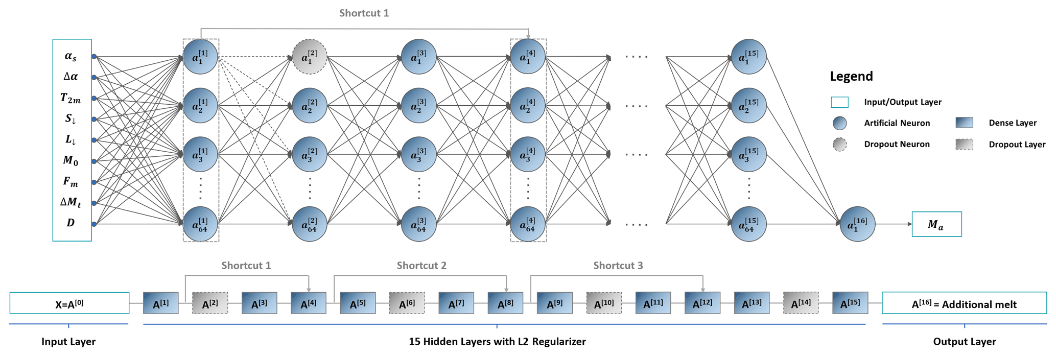
Figure 3Overview of the built deep multilayer perceptron (MLP) model architecture; the input parameters are the simulated albedo (αs) itself, the albedo difference () between the observed (αo) and simulated albedo, air temperature at 2 m (T2 m), incoming shortwave radiation (S↓), downwelling longwave radiation (L↓), simulated surface melt (M0), Boolean melt flag (Fm), surface melt difference to the previous day (ΔMt), and record date as day of the year (D).
Additionally, for comparison purposes, we have also built a multivariate linear regression model, a boosting model (XGBoost – a highly effective and widely used tree boosting system; Chen and Guestrin, 2016), a bagging model (random forest; Breiman, 2001), and a shallow MLP model (single hidden layer with 12 neurons). The bagging and boosting models are developed in Python using the open-source scikit-learn and XGBoost packages, and the shallow MLP model is developed using Keras. To tune the hyperparameters in the random forest and XGBoost model, the GridSearchCV function built in scikit-learn is used. Validation of the abovementioned models is implemented by comparing the accuracy metrics based on the training and validation data sets. To evaluate the deep MLP model and the other machine/deep learning models, we have separated the augmented AWS observations (Sect. 3.3) into a training data set containing AWS 14 and AWS 17 and a validation data set consisting of AWS 18. Afterward, three metrics are calculated to evaluate the model performance: the root-mean-square error (RMSE), the mean absolute error (MAE), and the coefficient of determination (R2).
3.5 MODIS albedo correction and interpolation
When the deep learning model is applied to RACMO2 output, corrections to surface melt are guided by MODIS observations of surface albedo. Therefore, we use the MODIS albedo product (MCD43A3), which is a clear-sky product based on observed clear-sky surface reflectances from the Level 2 Surface Reflectance product (MOD09, MYD09). Hence, the MODIS white-sky albedo needs to be converted to blue-sky albedo by correcting for the influence of changing solar zenith angle and cloud cover, both of which have a significant impact on surface albedo over snow (Kuipers Munneke et al., 2008). Therefore, we use MODIS white-sky albedo as diffuse albedo αs at 50∘ and apply the RACMO2 parametrization for solar zenith correction (dαu) and clouds (dατ), as described in Kuipers Munneke et al. (2011) and developed in Gardner and Sharp (2010). This requires the cloud optical depth and solar zenith angle as input. The latter is computed as a function of date and geographical location. Cloud optical depth (τ) is calculated from RACMO2 simulations of the ice water path (IWP) and liquid water path (LWP) using the parameterization from Stephens (1978):
where the subscripts “i” and “w” denote a separate treatment for ice and water. The total cloud optical depth is
The effective particle radius used for ice (Reff,i) and water (Reff,w) is 30 µm and 13 µm, respectively (Henderson et al., 2011). The respective densities are ρi=916.7 kg m−3 and ρw=1000 kg m−3. IWP and LWP (kg m−2) are the respective integrated cloud ice and water content over cloud depth z, under the assumption that the cloud is vertically uniform with respect to the drop-size distribution (i.e., well mixed). Although this is a simplified assumption, it allows a first-order correction for cloud effects on the satellite albedo. After this correction, the daily total-sky MODIS albedo values were derived. We then implemented a linear interpolation over time to fill in missing values caused by persistent cloud obstructions (with a frequency of 15.51 % at AWS 14, 8.45 % at AWS 17, and 1.32 % at AWS 18).
3.6 Application of the MLP model to RACMO2
As our objective is to improve surface melt simulations from RACMO2 over all Larsen ice shelves, it is vital to assess the MLP model performance with respect to both the reference data set and the RACMO2 simulations directly. For the reference data set, we use the AWS data and perturbed albedo changes as input data for Eq. (2), whereas for the RACMO2 simulations, we rely on RACMO2 data and MODIS albedo observations as inputs to calculate the corrected surface melt (Mc):
where M0 represents the uncorrected surface melt simulations for both the reference and RACMO2 data sets, and Ma stands for the additional surface melt estimated by the deep MLP model. Additionally, to calibrate overcorrections, if the corrected surface melt is negative, we have set it to zero using Eq. (6). Outside of the austral summer, when absorbed solar radiation is no longer the major source of energy for surface melt, the deep MLP model is switched off, and the original RACMO2 simulations are used to calculate the annual surface melt.
The correction can be performed to be consistent with the temporal extent of the MCD43A3 product (i.e., from 16 February 2000 to present). However, to intercompare the original RACMO2 surface melt, the corrected surface melt, and the AWS observations, the application in this study is limited to 2009–2016 – the period for which AWSs were operated on the Larsen Ice Shelf (Fig. 1).
3.7 Evaluation of the MLP model performance
To evaluate the deep MLP model performance, we conduct two separate analyses. The first evaluation focuses on the robustness of the method that we developed. In Sect. 4.1, we assess the deep MLP model performance using a cross-validation, i.e., we evaluate if the deep MLP model is able to recreate the time series of surface melt from the surface energy balance model. We set aside the reference data set at AWS 18 as the validation data set, thereby preserving the complete inter- and intra-annual melt variability. In the same way, we also benchmark the deep MLP model with other machine learning models: a multivariate linear regression model, an XGBoost model (a leading boosting machine learning model), a random forest regression (a leading bagging machine learning model), and a shallow MLP model containing only one hidden layer and few neurons (hereafter referred to as a shallow MLP model).
The second analysis, presented in Sect. 4.3, assesses the performance of the deep MLP model in the final application to RACMO2 model simulations that are corrected using MODIS albedo observations. First, we thoroughly evaluate MODIS albedo in an intercomparison with AWS and RACMO2 albedo before we use it as an input to the deep MLP model. This can reveal potential sources of error from the input albedo in the deep MLP model application and also demonstrates discrepancies among the three data sets at different AWS locations. Second, we apply the deep MLP model to MODIS and RACMO2 data, and present the corrected surface melt in section 4.3, along with the AWS observations, QuikSCAT-based estimations (Trusel et al., 2013), and original RACMO2 simulations over the Larsen Ice Shelf (AWS 14, AWS 17, and AWS 18). Additionally, to further investigate the potential influence of the imprecise meteorological input parameters to the deep MLP model, we display the contemporary T2 m, S↓, L↓, and α from AWS observations, RACMO2 simulations, and/or MODIS observations.
4.1 MLP performance: application of the MLP to AWS data
Here, we test the technical correctness of the deep MLP model as well as its ability to learn the behavior of the surface energy balance model. We first present the cross-validation results, indicating the performance of the deep MLP model when applied to data from a different location. Subsequently, we compare the performance of the deep MLP to other machine learning models. Finally, we present the capacity of the developed MLP model to reconstruct the time series of surface melt from the surface energy balance model.

Figure 4Performance of the deep multilayer perceptron (MLP) model regarding its (a) overall accuracy, (b) accuracy of melt periods, (c) accuracy of no-melt periods, (d) accuracy in each month (as no melt event occurred in June during the automatic weather station (AWS) operation period based on the AWS observations, the June value is absent), (e) accuracy for all albedo differences, and (f) monthly accuracy (in terms of the additional melt). RMSE, MAE, R2, DOY, and Δα stand for the root-mean-square error, the mean absolute error, the coefficient of determination, the day of the year, and the albedo difference, respectively.
4.1.1 Accuracy assessment based on cross-validation
The cross-validation of the additional daily surface melt (Ma) predicted by the deep MLP model (Fig. 4a) shows a high correlation (R2=0.95) between the deep-MLP-modeled Ma and that from the surface energy balance calculations based on the perturbed observations at AWS 18. The overall RMSE and MAE are 0.95 and 0.42 mm w.e. d−1, respectively. However, no- and low-melt values are abundant, and they can greatly reduce the errors, especially outside of the summer season. To eliminate such an effect, we discriminate between melt and no-melt periods, and the results are summarized separately in Fig. 4b and c. During melt periods, errors are 1.05 (RMSE) and 0.70 mm w.e. d−1 (MAE). These values are higher than for the no-melt periods, which have an RMSE and MAE of 0.91 and 0.34 mm w.e. d−1, respectively. The R2 is 0.24 lower under no-melt conditions than under melt conditions because of a number of notable outliers during no-melt periods (Fig. 4c). These outliers indicate that the deep MLP model sometimes has issues simulating low values of additional melt (Fig. 4a–c), leading to a “sword-like” pattern in Fig. 4a. The points along/close to the x and y axes mainly originate from no-melt periods (Fig. 4c). Such errors mostly occur when Δα is smaller than −0.2 during no-melt periods (red circles in Fig. 4c), which is rare in reality. In such cases, the deep MLP model is more likely to set the surface melt back to zero. The second type of error is the horizontal line crossing the origin. This mainly occurs during melt periods in winter, between approximately May and August. The deep MLP model does not know how to behave, as solar radiation is absent and albedo is undefined: Δα is no longer the dominant factor that influences the magnitude of the surface melt. This is confirmed by the winter melt anomalies in 2016 (see Sect. 4.1.3). Assessment of the model performance throughout the year (Fig. 4d) illustrates a “bowl-like” pattern for the overall accuracy and the accuracy for no-melt periods, with RMSEs close to zero during the no-melt periods. During the melt season, RMSEs are close to 1.0 mm w.e. d−1. In Fig. 4e, the model accuracy for different Δα shows a minimum for Δα equals zero. The higher the absolute value of Δα, the higher the RMSE and MAE. Lastly, when daily values of surface melt are aggregated to monthly surface melt, the accuracy of the deep MLP model increases strongly (R2=0.99). This suggests that it is more appropriate to utilize the monthly results.
4.1.2 Performance of machine learning and deep learning model
The deep MLP model generally outperforms other machine learning models (Table 1). The performance of the multivariate linear regression model is weakest, i.e., the highest RMSE and MAE as well as the lowest R2. The commonly used random forest and XGBoost models both outperform the multivariate linear regression model and the shallow MLP model. Furthermore, they are less likely to overfit after the hyperparameter tuning and regularization. In particular, random forest regression has achieved a slightly better MAE and R2 than the deep MLP model in the validation data set. In comparison to the shallow MLP architecture, the deep MLP with stricter regularization and shortcuts shows a noticeable improvement in accuracy. Thus, we demonstrate that a lot of improvement can be achieved by customizing and optimizing a deep learning model compared with using an off-the-shelf model. This confirms that the deep neural network can improve the surface melt simulations from RACMO2 over the Larsen Ice Shelf when accurate meteorological input data are available.
Table 1Performance of different models in estimating additional melt from the regional atmospheric climate model version 2.3p2 (RACMO2) simulations. The training data set is the augmented automatic weather station (AWS) observations from AWS 14 and AWS 17, and the validation data set is the augmented AWS observations from AWS 18.
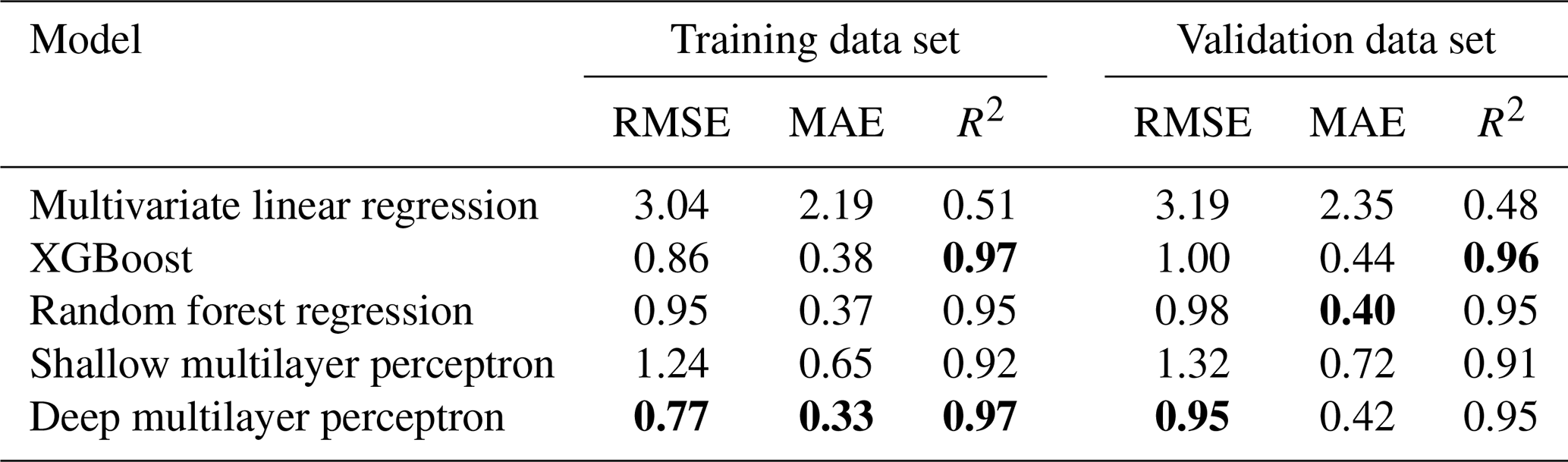
RMSE, MAE, and R2 stand for the root-mean-square error, the mean absolute error, and the coefficient of determination, respectively. The bold values indicate the best results with respect to RMSE, MAE, and R2.
4.1.3 Time series of MLP-predicted surface melt
The time series of corrected surface melt for different Δα values show that lower Δα values lead to higher daily surface melt (Fig. 5), except for melt events during the wintertime in 2016 (Fig. 5a). Figure 5b reveals that the disparity between the deep-MLP-predicted surface melt and the augmented AWS observations increases with the drop in albedo, especially when . The time series show that most surface melt occurs during the austral summer. The largest differences between the deep-MLP-predicted surface melt and the augmented AWS observations are mainly found during peak episodes of melt. It is also noteworthy that the daily surface melt difference among different Δα values is larger than the difference between the deep MLP results and (perturbed) AWS observations which indicates that the albedo is the main source of uncertainty, not the uncertainties from the deep MLP model.
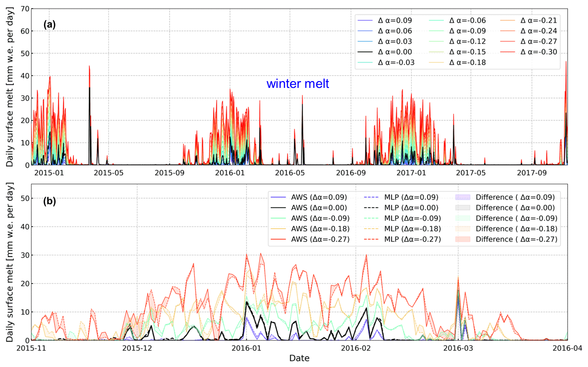
Figure 5Temporal changes in the corrected regional atmospheric climate model version 2.3p2 (RACMO2) surface melt using the deep multilayer perceptron (MLP) model at automatic weather station (AWS) 18, (a) for all albedo differences (Δα) and (b) for a subset between November 2015 and April 2016 along with the augmented AWS observations for comparison.
As shown in Fig. 5a, there is a period of anomalously high surface melt during the winter of 2016, demonstrated previously in AWS and satellite observations as well as in RACMO2 simulations (Kuipers Munneke et al., 2018a). In the deep MLP results, the winter melt episodes are almost identical for different Δα values. Given that winter melt events occurred during polar darkness, the incoming shortwave radiation is almost zero. In such circumstances, the incoming shortwave radiation is no longer the key factor leading to a surface melt increment. Therefore, Δα no longer influences such winter melt events. The actual trigger for the winter melt events is föhn winds, adiabatically heated winds that descend from the Antarctic Peninsula mountains to the west of the Larsen Ice Shelf (Marshall et al., 2006; Orr et al., 2008; Cape et al., 2015).
In Fig. 5b, we demonstrate that the deep MLP model is capable of not only enhancing existing melt but also of simulating melt when there was no melt in the original time series. When Δα exceeds a certain value, the overall temporal melt pattern differs from that for lower Δα values. This results in a longer-lasting and more intense melt event. Moreover, because of the dependence of melt on the occurrence of melt on the previous day, the duration of a certain melt event may be prolonged. This simulates a melt–albedo feedback: an initial melt event may trigger a melt event the next day, as albedo is reduced.

Figure 6Scatterplots illustrating albedo difference under clear-sky conditions during austral summers between automatic weather station (AWS) and Moderate Resolution Imaging Spectroradiometer (MODIS) observations, and albedo difference between AWS observations and regional atmospheric climate model version 2.3p2 (RACMO2) simulations in (a) AWS 14, (b) AWS 17, and (c) AWS 18, along with their corresponding distributions in (d) AWS 14, (e) AWS 17, and (f) AWS 18. RMSE and R2 stand for the root-mean-square error and the coefficient of determination, respectively.
4.2 Comparing albedos from MODIS, AWS, and RACMO2
For clear-sky conditions indicated by MOD09GA (Fig. 6), AWS 14 and AWS 17 show higher correlations with MODIS (R2 values of 0.28 and 0.20, respectively) than RACMO2 (R2 values of 0.17 and 0.02, respectively), whereas this is reversed for AWS 18, with better correlations between AWS and RACMO2 (R2 of 0.40). The RMSE between AWS and MODIS is lower than the RMSE between AWS and RACMO2 at AWS 14 (by <0.01) and AWS 17 (by 0.01), but it is 0.02 higher at AWS 18. Histograms of albedo values are shown in Fig. 6d–f. At AWS 14, both MODIS and RACMO2 show higher values of albedo than AWS observations. For lower albedo values, AWS observations agree better with RACMO2 simulations than with MODIS observations. Even though the three data sets have a similar range of albedo values, the MODIS albedo observations are narrow and less skewed. At AWS 17, AWS observations show a broad distribution and are mostly below 0.85. They agree better with the MODIS observations than with RACMO2 simulations. At AWS 18, MODIS observations are lower than AWS observations and RACMO2 simulations, and RACMO2 simulations are more similar to AWS observations.
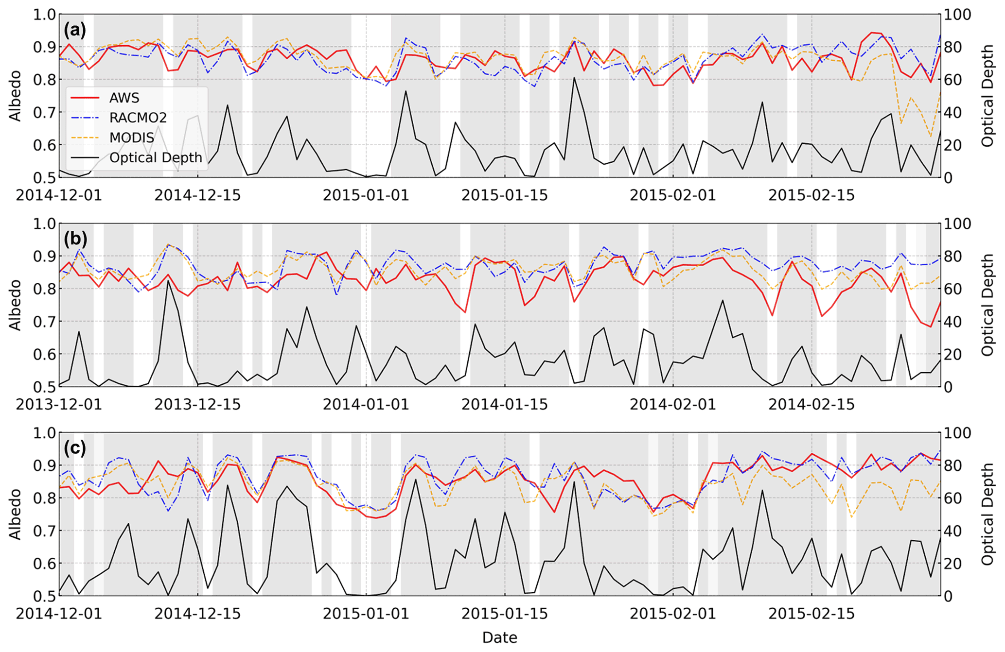
Figure 7Temporal changes in albedo from the regional atmospheric climate model version 2.3p2 (RACMO2) simulations, automatic weather station (AWS) observations, and Moderate Resolution Imaging Spectroradiometer (MODIS) observations at AWS 14, AWS 17, and AWS 18 during the austral summer 2014–2015, 2013–2014, and 2014–2015, respectively. The gray bars indicate the binary cloudiness of a 500×500 MODIS pixel corresponding to each AWS location.
Typical time series of albedo from RACMO2, AWSs, and MODIS show that the differences between the three albedo products are relatively small during most of the austral summer season (Fig. 7). The RMSEs between AWS-observed and MODIS-observed albedo as well as between AWS-observed and RACMO2-simulated albedo in December and January are around 3.5 % (AWS 14), 5.5 % (AWS 17), and 4.5 % (AWS 18). The RMSE between AWS-observed and RACMO2-simulated albedo increases up to 8.8 % (AWS 17) in February. On a daily basis, for the first half of December, MODIS-observed and RACMO2-simulated albedo values are comparably high at AWS 17, 4.5 % (RACMO2) and 8.5 % (MODIS) higher than AWS observations on 11 December 2013 (Fig. 7b), and at AWS 18, 6.8 % (RACMO2) and 3.5 % (MODIS) higher than AWS observations on 6 December 2014 (Fig. 7c). The contemporary optical depth is also relatively high (15.64 at AWS 17 and 16.76 at AWS 18). In contrast, at AWS 18 on 12 December 2014, both MODIS-observed and RACMO2-simulated albedo values are comparably low, 11.4 % (RACMO2) and 7.4 % (MODIS) lower than AWS observations, and the optical depth is close to zero on a cloudy day. The difference remains low during the middle of the summer season but gradually increases (up to 19.18 % between RACMO2 and AWS observations at AWS 17 on 27 February 2014) towards the end of the summer season in February. RACMO2 simulations tend to produce the highest albedo at the three AWSs on average. At AWS 14 and AWS 18, RACMO2 simulations are more consistent with the AWS observations than with MODIS observations (Fig. 7a, c). MODIS observations are comparably lower than AWS observations and RACMO2 simulations at the end of February. On the contrary, AWS observations are much lower than RACMO2 simulations at AWS 17 (Fig. 7b). For albedo values higher than 0.80, AWS observations and MODIS observations are similar, but for albedo below 0.80, AWS observations show a broader tail towards lower values (e.g., as shown in Fig. 7a at AWS 14 at the end of February 2014). It is noteworthy that each AWS has different background geophysical settings, and the three products have very different spatial resolutions: AWS observations are local in situ observations, whereas MODIS albedo observations and RACMO2 albedo simulations have a 27 km spatial resolution. Further analyses and discussion can be found in Sect. 5.1.
To translate the white-sky MODIS albedo to the blue-sky albedo, we used the optical depth simulated by RACMO2 at its horizontal resolution of 27 km. The optical depth from RACMO2 and the cloudiness from the MOD09GA product are displayed in Fig. 7 for AWS 14, AWS 17, and AWS 18. The optical depth from the RACMO2 simulations is often close to zero on clear-sky days; however, there are more erroneously high optical depth values observed at AWS 18 than at AWS 14 and AWS 17. This is because RACMO2 provides daily average IWP and LWP values, but the RACMO2.3p2 version has a systematic overestimation of both cloud ice and water, simulating clouds that are optically too thick. The general biases in these cloud variables are especially large for the coastal bins (Fig. 6b in van Wessem et al., 2018), possibly explaining the erroneously high optical depth observed at AWS 14 and AWS 17 (Fig. 7), in which clouds are considered “thin” when τ≤6 or “thick” when τ≥12. The interpretation of albedo differences in this section is also hampered because values from different sources are representative of areas of very different sizes. An AWS observation has a spatial footprint of the order of 10×10 m2, whereas the RACMO2 and MODIS values represent an area of hundreds of square kilometers. We demonstrate the possible consequences for each AWS location using high-resolution maps of Sentinel-1 backscatter (Fig. 8), which is produced following Luckman et al. (2014). The orange and red pixels represent the detected melt based on dB, where is the backscatter value for a pixel observed on a certain date (t), and is the mean backscatter between June and August (Luckman et al., 2014; Trusel et al., 2012).
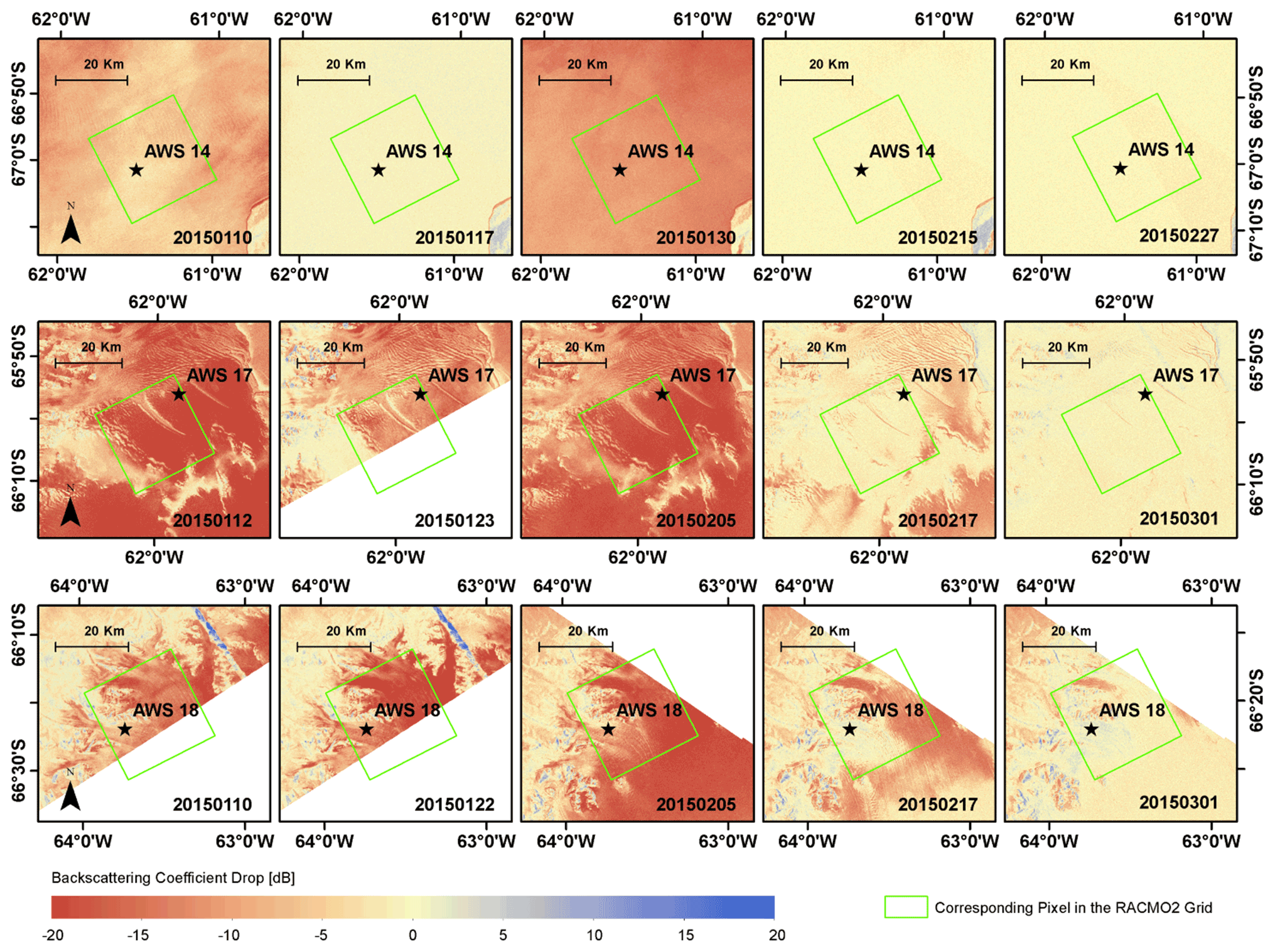
Figure 8Spatiotemporal patterns of surface melt, represented by the drop in the backscattering coefficient in Sentinel-1 imagery, in automatic weather station (AWS) 14, AWS 17, and AWS 18 observations between January and March in 2015 as well as their corresponding regional atmospheric climate model version 2.3p2 (RACMO2) pixels.
4.3 MLP performance: application of the MLP to RACMO2 and MODIS data
At AWS 14, the discrepancies between the AWS observations and RACMO2 simulations with respect to the 2 m air temperature and incoming shortwave radiation are the smallest amongst the three AWSs (Fig. 9a). This potentially reduces the effects of these meteorological parameters on the surface melt in addition to albedo. On a daily basis (Fig. 9b), the deep MLP model tries to make the melt agree more with observations at AWS 14, although it is difficult for the deep MLP model to alter the RACMO2 melt signal significantly. Therefore both the RACMO2 and MODIS albedo data remain similar. It is noteworthy that a melt event at the beginning of February 2014 is erroneously corrected by the deep MLP model, as both AWS and RACMO2 do not observe or simulate such a melt event. This is plausibly due to the significantly higher temperature simulated by RACMO2 than the one observed by AWS (Fig. 9a). The contemporary albedo simulations/observations agree well among the three data sets. However, RACMO2 simulates higher 2 m air temperature. Therefore, we assume that the developed deep MLP model and its “learned” melt mechanism are also sensitive to the other input meteorological parameters, such as 2 m air temperature. Furthermore, the discrepancy at the daily scale seems to originate from a different timing of melt in both RACMO2 and the observations. The deep MLP model is unable to completely repair the timing offset, which is different from the observations. When considering longer-term averages, the deep MLP model delivers an improvement of the melt fluxes. Figure 9c shows a closer agreement of the deep MLP model with AWS observations for monthly melt fluxes. Moreover, for annual fluxes, both the deep MLP model and RACMO2 annual melt fluxes are higher than in the AWS observations, although both are close to the QuikSCAT estimates.
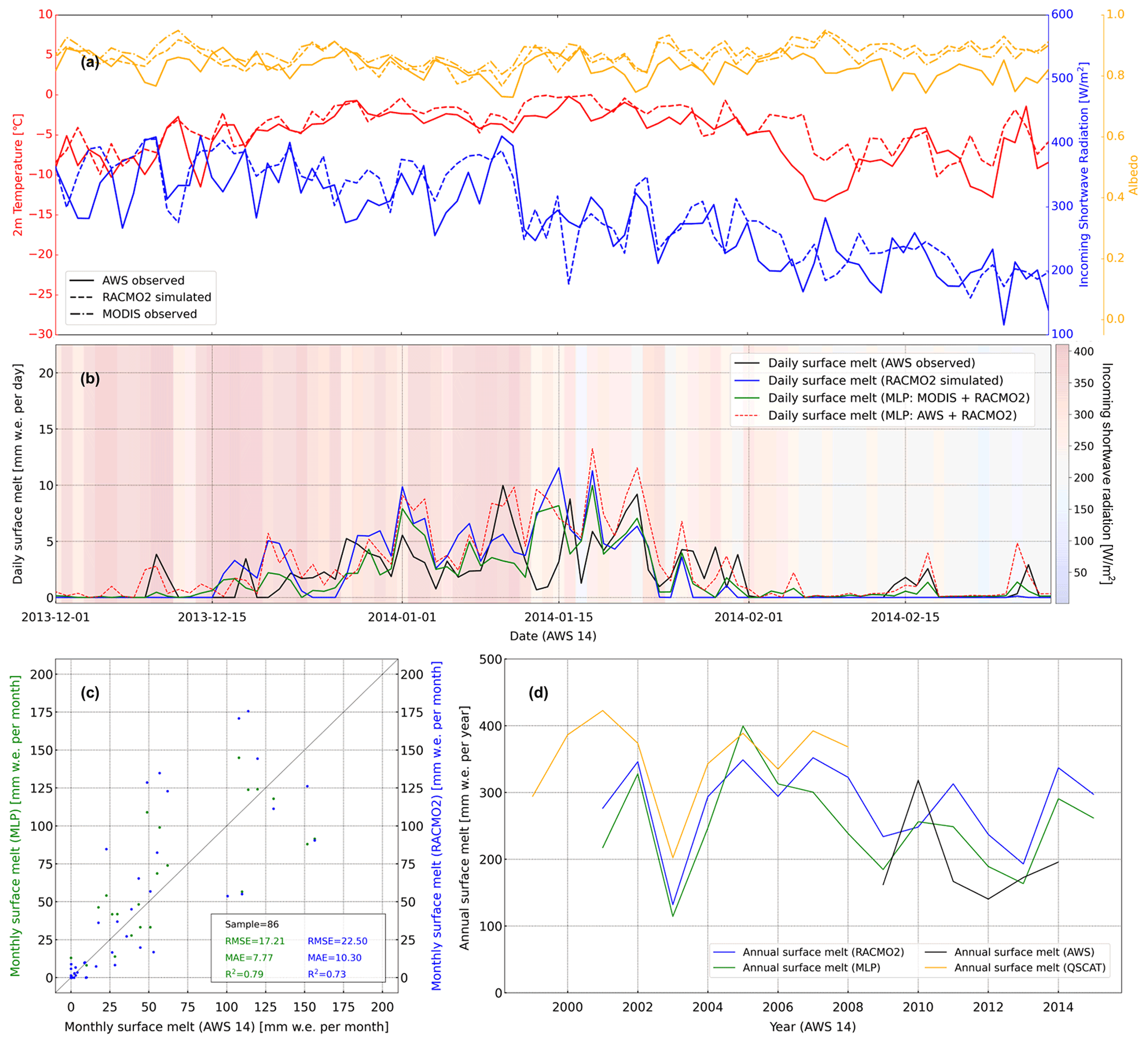
Figure 9Automatic weather station (AWS) observations, regional atmospheric climate model version 2.3p2 (RACMO2) simulations, and results of the deep multilayer perceptron (MLP) model applied to RACMO2 and Moderate Resolution Imaging Spectroradiometer (MODIS) data at AWS 14: (a) discrepancies in input meteorological parameters among the AWS observations, RACMO2 simulations, and MODIS observations; (b) daily surface melt time series from the original RACMO2 simulations, AWS observations, and MLP estimations using a different input data set for albedo (from either MODIS or AWS observations) and the other meteorological parameters from RACMO2 during the austral summer 2013–2014; (c) a scatterplot of monthly surface melt from the deep MLP model estimations and the original RACMO2 simulations compared to AWS observations; and (d) annual melt fluxes (July–June) at AWS 14 from AWS observations, RACMO2 simulations, the deep MLP predictions, and QuikSCAT (Quick Scatterometer) estimations (Trusel et al., 2013).
At AWS 17, RACMO2 shows a systematic overestimation of air temperature and incoming shortwave radiation compared with AWS observations (Fig. 10a). Consequently, it leads to apparent overestimations of surface melt in RACMO2 simulations in December 2013 (Fig. 10b), when the discrepancy in albedo is small. During the middle of the austral summer 2013–2014, replacing the MODIS-observed albedo by the AWS-observed albedo in the deep MLP model input results in a better agreement with the AWS surface melt observations. This reveals the potential of improving the deep MLP model accuracy by better estimating the surface albedo from MODIS. At AWS 17 during the end of February 2014, when AWS observed two extensive melt events, RACMO2 simulates the incoming shortwave radiation well. However, even when replacing the MODIS albedo observations with AWS observations in the deep MLP model input, the mismatch is still significant. It seems that the underestimations in the 2 m air temperature are the trigger. Therefore, attention should be paid to other influencing meteorological parameters in addition to albedo. Although the deep MLP model improves the estimate of monthly surface melt (Fig. 10c) and brings annual melt more in line with QuikSCAT (Fig. 10d), compared with the AWS observations, both the deep MLP model and RACMO2 annual melt are much lower (Fig. 10d).
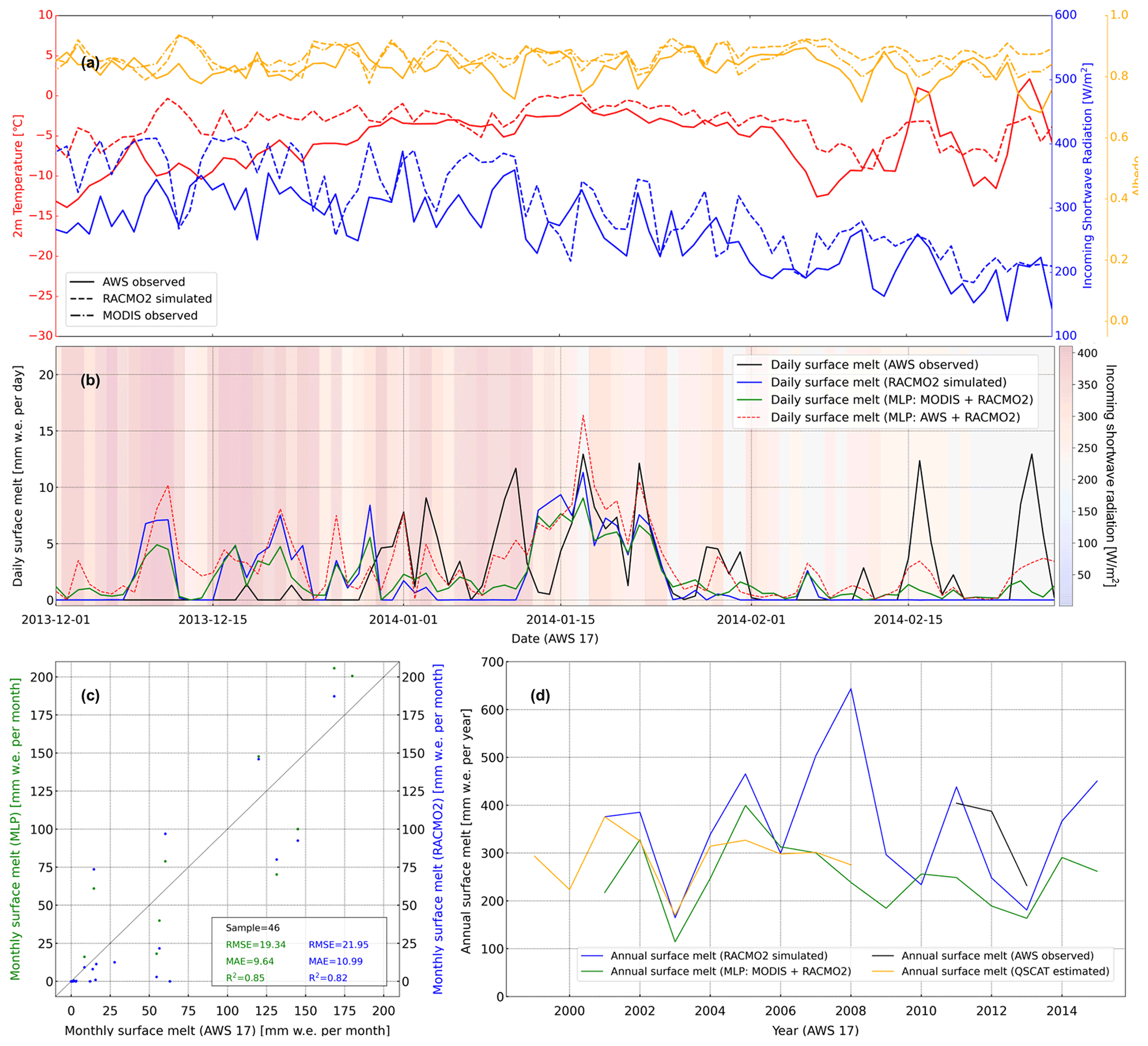
Figure 10The same as Fig. 9 but for AWS 17.
At AWS 18, the deep MLP model fails to improve surface melt compared with observations. Instead of reducing the overestimations of the original RACMO2 simulations in the daily surface melt, the deep MLP model tends to further increase the daily surface melt (Fig. 11b). This is plausibly due to the overestimations in the 2 m air temperature by the RACMO2 simulations (Fig. 11a). Furthermore, using AWS-observed albedo instead of MODIS-observed albedo shows an improvement in the agreement with AWS surface melt. This is either due to imprecise MODIS albedo or great spatiotemporal variance between the surface melt at AWS 18 and its corresponding RACMO2 pixel. On the other hand, it indicates that the deep MLP model does not always reduce the surface melt simulations and can also increase surface melt simulations. In the end, both the RMSE and MAE increase by 11.32 and 7.87 mm w.e. per month after the correction using the deep MLP model applied to RAMCO2 and MODIS data (Fig. 11c). The discrepancies are also shown in the comparison of the annual surface melt, in which the deep MLP model produces the highest estimations throughout all of the years. QuikSCAT estimates and AWS observations are the lowest (Fig. 11d). Moreover, this discrepancy indicates the importance of high-spatial-resolution corrections. At the 27 km resolution, the MODIS albedo is often lower than the RACMO2 albedo, resulting in increased melt. At the point scale of the AWS, the AWS albedo is higher than the RACMO2 albedo, resulting in decreased melt. This indicates that the spatial scale of corrections (27 km versus local scale) matters.
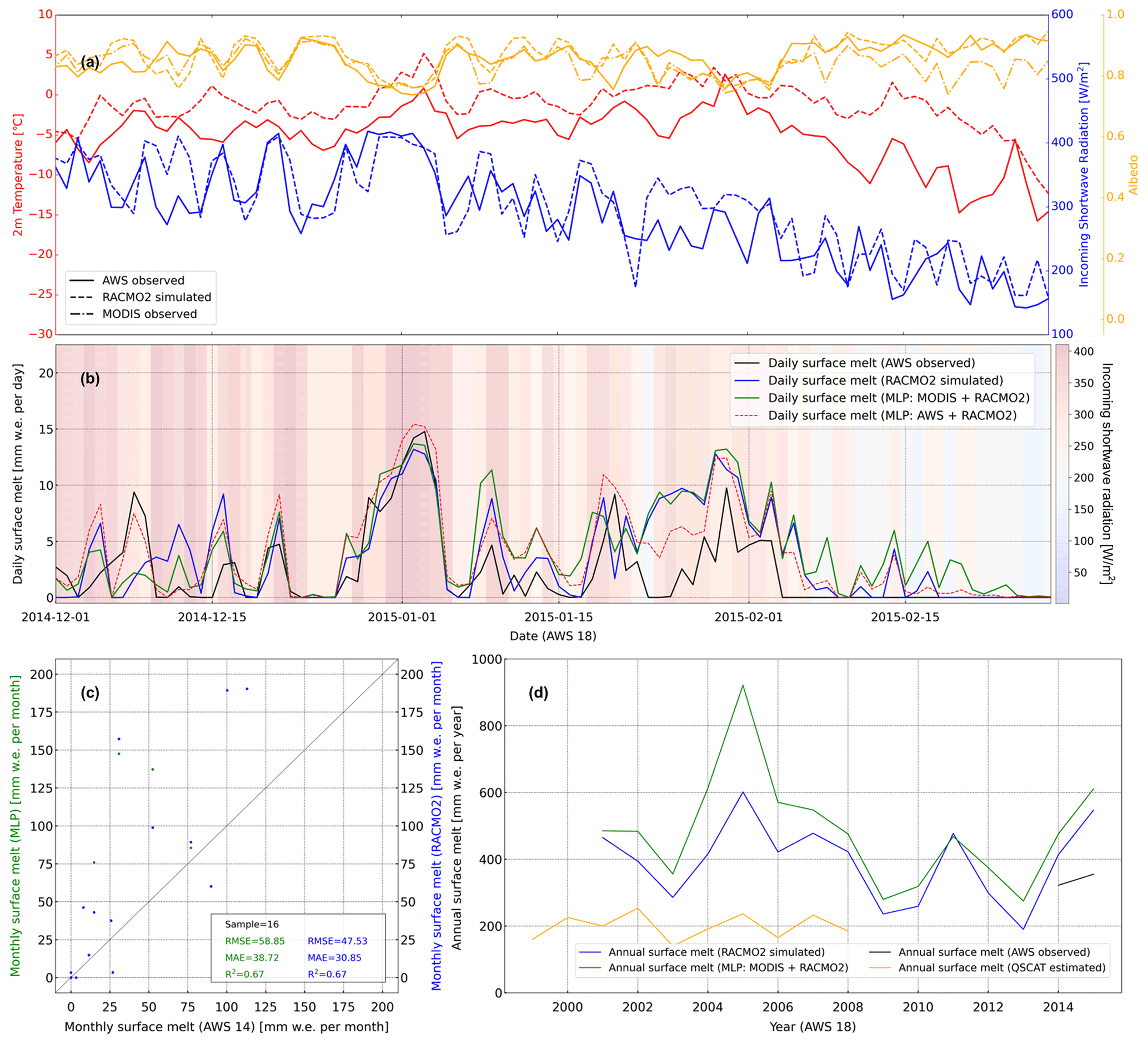
Figure 11The same as Fig. 9 but for AWS 18 during the austral summer 2014–2015 in (a) and (b).
5.1 Impacts of different geophysical settings on MLP model performance
The developed MLP model shows good performance for the ideal scenario, i.e., when only the albedo observations from an AWS are perturbed by an amount Δα (see Sect. 3.3). Its performance has been evaluated by a cross-validation based on the reference data set at AWS 18, for different Δα values for both melt and no-melt periods. The performance of the deep MLP model is good especially during the austral summer, when most of the melt events take place, caused mainly by solar radiation modulated by surface albedo. When replacing the AWS observations by MODIS observations and RACMO2 simulations, the deep MLP performance is more difficult to establish (Sect. 4.3) and varies for different AWS locations. The first complicating factor is our assumption that albedo is the main driver of surface melt differences. Although we assumed that Δα is the key factor in surface melt variation during the austral summer in Antarctica, surface melt is actually also determined by other meteorological parameters (e.g., air temperature), which can be biased in RACMO2 (Sect. 4.3). As a second complicating factor, the performance of the deep MLP model is compromised because of systematic biases in MODIS albedo compared with AWS observations. It seems that the geophysical setting (geolocation, surface type, melt pattern, topographical characteristics) play an important role in both of these factors. Therefore, we discuss the geophysical settings of AWS 14, AWS 17, and AWS 18 in order to explain the deep MLP results.
Scenario 1 (AWS 14): AWS 14 and its corresponding RACMO2 pixel are centrally located in the northern part of the Larsen C Ice Shelf, where the terrain is flat, homogeneous, and covered by snow and firn. At AWS 14, albedo is relatively well simulated by RACMO2, and the discrepancies among the three albedo data sets are low throughout the austral summer (Fig. 7). No constant over- or underestimations in albedo have been found in MODIS observations and RACMO2 simulations, compared with AWS observations. Owing to the homogeneous geophysical settings, its spatiotemporal melt pattern is homogeneous as well. Therefore, when applying the deep MLP model to RACMO2 and MODIS, the result shows a better agreement with the AWS observations at AWS 14 than at AWS 17 and AWS 18.
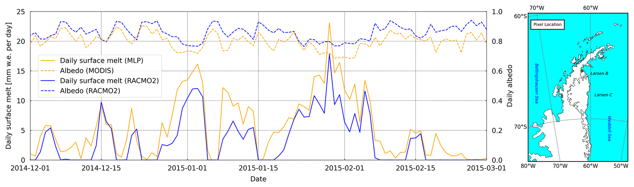
Figure 12Daily surface melt from regional atmospheric climate model version 2.3p2 (RACMO2) simulations and multilayer perceptron (MLP) estimations, albedo from RACMO2 and MODIS at the additional test site in the north of AWS 17 (left panel), and the geolocation of the test site (i.e., the red square in the right panel). The shapefiles of the Antarctic coastline and ice shelves are provided by the Scientific Committee on Antarctic Research Antarctic Digital Database (SCAR ADD; https://www.add.scar.org/, last access: 11 November 2021).
Scenario 2 (AWS 17): AWS 17 is located in the middle of Scar Inlet, a remainder of the Larsen B Ice Shelf, where the terrain is flat. However, its corresponding RACMO2 pixel also contains the grounded areas at the edge of the pixel and partially covers mountainous terrain. The albedo discrepancy is the largest amongst the three data sets (i.e., AWS observations, MODIS observations, and RACMO2 simulations). At the point level, AWS 17 is located in the most extensive melt area, resulting in AWS observations that are constantly lower than both the MODIS observations and RACMO2 simulations for a 27 km pixel. On the other hand, albedo from RACMO2 simulations and MODIS observations remains close, as the proportion of the grounding line and mountains is low in the pixel. Therefore, the deep MLP model results agree less than those at AWS 14.
Scenario 3 (AWS 18): AWS 18 is situated in an inlet near the grounding line of the Larsen C Ice Shelf; the surrounding area consists of complex terrain and also contains grounded areas. Its corresponding RACMO2 pixel is the most mixed pixel among the three AWS locations, and melt ponds can occur during melt events. The AWS at this location does record extensive melt events, but it is not located in the area of strongest melt in the RACMO2 pixel. The discrepancies in albedo from the three data sets are small at the beginning and the middle of austral summer, but MODIS observes much lower albedo at the end of austral summer. The spatiotemporal melt pattern is also the most heterogeneous among the three AWS locations. Apart from the Δα, the terrain itself also impacts the surface melt process. In the end, the challenges in accurately deriving albedo at AWS 18 and the combination of multiple influencing factors result in poor performance of the deep MLP model. Furthermore, attention must be paid to the representativeness of the AWS observations in such an area, which makes the verification difficult.
Scenario 4 (additional site north of AWS 17): the last scenario is an additional location north of AWS 17 on Scar Inlet, sitting on the grounding line of the Larsen B Ice Shelf (Fig. 12). Such a location presents an ideal scenario, as the albedo observed by MODIS in this area is systematically lower than RACMO2 simulations (Fig. 12). This is a situation that the deep MLP model is actually designed for. As a result, the daily surface melt corrected by the deep MLP model is also systematically higher than the original RACMO2 simulation. Thus, it is an ideal area to illustrate the expected performance of the deep MLP model where the overestimation in surface albedo is the dominant factor causing surface melt underestimation in RACMO2. However, we do lack AWS observations to evaluate MLP performance at this location.
5.2 Lessons learned from this study over the Larsen Ice Shelf
Our study shows that the deep MLP model has the potential to improve surface melt estimates in Antarctica. On the other hand, the results at AWS 18 shed light on the fact that complicated and heterogeneous terrains can result in poor performance from the deep MLP model. AWS 18 is a typical area that has high-melt features, which we are interested in, but such high-melt features are usually of small scale. Although AWS observations suggest that there is an overestimation in albedo simulations from RACMO2, it is challenging for MODIS to correct it when implemented in a coarse-resolution climate model. Therefore, we need to combine the low-resolution RACMO2 data with higher-resolution MODIS data to resolve this issue. Moreover, there is also the potential to further increase the resolving power of our method, including (1) a further refinement of the deep-learning-based framework; (2) improvement of the albedo derivation from satellite observations, both in magnitude and spatial resolution; and (3) examination of MLP model performance over (blue) ice surfaces.
Refinement of the deep-learning-based framework includes the development of a module to switch the deep MLP correction as well as testing of the state-of-the-art deep learning architectures and models. Given that the concept of correcting surface melt in non-albedo-driven areas may reduce the agreement between the AWS observations and RACMO2 simulations, it is necessary to develop an application strategy for deciding whether the deep MLP correction should be applied in a certain area. The strategy can take topographical characteristics (e.g., elevation, aspect, slope), albedo difference, and geolocation into consideration, as these factors can be influential (Sect. 5.1). It is also worth mentioning that the deep learning model implemented in this study is fundamental in order to prove the concept. Exploring other state-of-the-art deep learning architectures and models, e.g., applying recurrent neural network architectures such as long short-term memory (LSTM; Hochreiter and Schmidhuber, 1997) and transformer (Vaswani et al., 2017) to help the deep learning model take in more temporal information, and/or using a convolutional neural network to generate a better representation of MODIS albedo information within a RACMO2 grid.
Improvement of the albedo derivation from satellite observations can result in better corrected surface melt results using the deep MLP model. Attention should be paid to the generation and correction of the MODIS albedo observations, as the MCD43A3 is a 16 d synthetic product. For a certain day, a composite 500 m resolution daily product is generated based on 16 d records centered on the given day (Schaaf and Wang, 2015). Temporal interpolation over long periods can lead to high disparity in the albedo during an ablation season, especially on high-melt days. Moreover, in heterogeneous terrain, such as the location of AWS 18, albedo may be highly different in space. Therefore, implementing a spatial resampling may improve this issue. Furthermore, the MODIS albedo correction for cloud cover based on optical depth from RACMO2 needs additional care, as RACMO2 overestimates optical depth at some locations.
On the Larsen Ice Shelf, reduction in albedo is mainly due to the aging of snow and firn. Yet, in icy areas (mainly on the ice shelves of eastern Antarctica and the Transantarctic Mountains), albedo reduction is much stronger than over firn and snow surfaces. Moreover, the surface energy balance over ice surface can be fundamentally different from that over firn and snow surfaces, for which the deep MLP model is trained in this study. Therefore, the deep MLP model performance in blue ice areas needs to be examined with extra care.
In addition to the improvement of the deep MLP model, we also need to look for novel and unconventional ways to validate results over unsurveyed areas. Earth observation satellites, such as Landsat, MODIS, and the Advanced Very High Resolution Radiometer (AVHRR), can provide temporal records of the land surface and its modification over the last decades at different spatial and temporal resolutions. Potentially, we can compare the surface melt outcomes to proxies from remotely sensed data, e.g., melting decibel days (Trusel et al., 2013), lake depth (Philpot, 1989), and volume (Moussavi et al., 2020).
This paper demonstrates that surface melt simulations from the regional climate model RACMO2 can be improved by deploying a deep learning model trained on automatic weather station (AWS) observations. The deep learning model takes meteorological parameters, day of the year, and the original RACMO2 surface melt simulations as the inputs. The cross-validation shows a good performance (RMSE of 0.95 mm w.e. d−1, MAE of 0.42 mm w.e. d−1, and R2 of 0.95) for the Larsen Ice Shelf based on the augmented AWS observations. Regarding accuracy, the deep learning model outperforms some leading machine learning models (random forest regression and XGBoost) and a shallow deep learning model. To address the problem regarding inaccurate albedo simulations from the RACMO2 model, MODIS albedo observations after cloud and solar zenith angle correction have been used. The corrected MODIS albedo observations show a better correlation with AWS observations than the RACMO2 simulations at AWS 14 and AWS 17. At AWS 18, large disparities have been identified between corrected MODIS albedo observations and AWS observations. Possible explanations for this are the local geophysical settings (including cloudiness, spatiotemporal melt pattern, and topographical characteristics) and imperfect albedo correction at AWS 18. Finally, to correct the surface melt simulations from RACMO2 over the entire Larsen Ice Shelf, the assessment of model performance in areas and periods without AWS observations is indispensable. For deep learning model application, meteorological parameters except for albedo from AWS observations are replaced by the RACMO2 simulations. The corrected MODIS albedo observations replace albedo observations from AWS. The results indicate that the deep learning model performs well in the area with a homogeneous spatiotemporal melt pattern (AWS 14) and in the area with a heterogeneous spatial melt pattern that is homogeneous through time (AWS 17). However, the model performance is highly uncertain in areas with a heterogeneous spatial melt pattern that varies through time (AWS 18) due to the inaccurate albedo input and the lack of ground truth data. In summary, the concept of correcting surface melt simulations from the regional climate model RACMO2 using deep learning is feasible. Nevertheless, future studies are still required to refine the deep-learning-based framework, improve the albedo derivation from satellite observations, examine the deep MLP model performance over (blue) ice surfaces, and develop a novel validation scheme.
The MODIS/Terra Surface Reflectance Daily L2G Global 1 km and 500 m SIN Grid product is available from the Land Processes Distributed Active Archive Center (LP DAAC) (https://doi.org/10.5067/MODIS/MOD09GA.006, Vermote and Wolfe, 2015). The MODIS/Terra + Aqua Albedo Daily L3 Global 500 m SIN Grid product is also available from LP DAAC (https://doi.org/10.5067/MODIS/MCD43A3.006, Schaaf and Wang, 2015). Sentinel-1 images are provided by the European Space Agency (ESA) (https://sentinel.esa.int/web/sentinel/sentinel-data-access ESA, 2021). Automatic weather station observations from AWS 14, 17, and 18 are available from https://doi.org/10.1594/PANGAEA.910473 (Jakobs et al., 2020b). RACMO2 simulations (https://www.projects.science.uu.nl/iceclimate/models/antarctica.php#2-1, IMAU, 2021) are provided by van Wessem et al. (2018) and are available upon request from the original authors. The developed model and its outcomes are free to download via Zenodo (https://doi.org/10.5281/zenodo.5769661, Hu et al., 2021).
ZH, PKM, and SL designed the study. PKM implemented the AWS perturbation; ZH, SL, and MI corrected the MODIS albedo; and ZH designed and trained the deep neural network architecture. ZH, PKM, SL, and MB carried out the quantitative analyses. PKM, SL, and MB discussed the deep neural network results. ZH and PKM wrote the paper with contributions from all co-authors.
The contact author has declared that neither they nor their co-author has any competing interests.
Publisher's note: Copernicus Publications remains neutral with regard to jurisdictional claims in published maps and institutional affiliations.
The authors would like to thank Luke D. Trusel for providing monthly surface melt estimations derived from QuikSCAT. This research was funded by the Netherlands Space Office (NSO; grant no. ALWGO.2018.039). Peter Kuipers Munneke is funded by the Netherlands Earth System Science Center (NESSC). Maaike Izeboud was supported by the Dutch Research Council (NWO)/Netherlands Space Office (grant no. ALWGO.2018.043).
This research has been supported by the Netherlands Space Office (grant no. ALWGO.2018.030). This publication was also supported by PROTECT. This project has received funding from the European Union's Horizon 2020 Research and Innovation program under grant agreement no. 869304, PROTECT contribution number 25.
This paper was edited by Thomas Mölg and reviewed by two anonymous referees.
Arthur, J. F., Stokes, C., Jamieson, S. S., Carr, J. R., and Leeson, A. A.: Recent understanding of Antarctic supraglacial lakes using satellite remote sensing, Prog. Phys. Geogr., 44, 837–869, 2020. a
Bindschadler, R., Choi, H., Wichlacz, A., Bingham, R., Bohlander, J., Brunt, K., Corr, H., Drews, R., Fricker, H., Hall, M., Hindmarsh, R., Kohler, J., Padman, L., Rack, W., Rotschky, G., Urbini, S., Vornberger, P., and Young, N.: Getting around Antarctica: new high-resolution mappings of the grounded and freely-floating boundaries of the Antarctic ice sheet created for the International Polar Year, The Cryosphere, 5, 569–588, https://doi.org/10.5194/tc-5-569-2011, 2011. a
Breiman, L.: Random forests, Mach. Learn., 45, 5–32, 2001. a
Cape, M., Vernet, M., Skvarca, P., Marinsek, S., Scambos, T., and Domack, E.: Foehn winds link climate-driven warming to ice shelf evolution in Antarctica, J. Geophys. Res.-Atmos., 120, 11–037, 2015. a
Chen, T. and Guestrin, C.: Xgboost: A scalable tree boosting system, in: Proceedings of the 22nd acm sigkdd international conference on knowledge discovery and data mining, 13–17 August 2016, San Francisco, California, USA, 785–794, 2016. a
Datta, R. T., Tedesco, M., Fettweis, X., Agosta, C., Lhermitte, S., Lenaerts, J. T., and Wever, N.: The effect of Foehn-induced surface melt on firn evolution over the northeast Antarctic peninsula, Geophys. Res. Lett., 46, 3822–3831, 2019. a, b
Elvidge, A. D. and Renfrew, I. A.: The causes of foehn warming in the lee of mountains, B. Am. Meteorol. Soc., 97, 455–466, 2016. a
ESA: Sentinel data, available at: https://sentinel.esa.int/web/sentinel/sentinel-data-access, last access: 10 December 2021. a
Fox-Kemper, B., Hewitt, H., Xiao, C., Aðalgeirsdóttir, G., Drijfhout, S., Edwards, T., Golledge, N., Hemer, M., Kopp, R., Krinner, G., Mix, A., Notz, S. N., Nurhati, I., Ruiz, L., Sallée, J.-B., Slangen, A., and Yu, Y.: Ocean, Cryosphere and Sea Level Change Supplementary Material, in: Climate Change 2021: The Physical Science Basis. Contribution of Working Group I to the Sixth Assessment Report of the Intergovernmental Panel on Climate Change, edited by: Masson-Delmotte, V., Zhai, P., Pirani, A., Connors, S. L., Péan, C., Berger, S., Caud, N., Chen, Y., Goldfarb, L., Gomis, M. I., Huang, M., Leitzell, K., Lonnoy, E., Matthews,J. B. R., Maycock, T. K., Waterfield, T., Yelekçi, O., Yu, R., and Zhou, B., Cambridge University Press, available at: https://www.ipcc.ch/, last access: 3 December 2021. a, b
Fürst, J. J., Durand, G., Gillet-Chaulet, F., Tavard, L., Rankl, M., Braun, M., and Gagliardini, O.: The safety band of Antarctic ice shelves, Nat. Clim. Change, 6, 479–482, 2016. a
Gardner, A. S. and Sharp, M. J.: A review of snow and ice albedo and the development of a new physically based broadband albedo parameterization, J. Geophys. Res., 115, F01009, https://doi.org/10.1029/2009JF001444, 2010. a
Gilbert, E. and Kittel, C.: Surface Melt and Runoff on Antarctic Ice Shelves at 1.5 ∘C, 2 ∘C, and 4 ∘C of Future Warming, Geophy. Res. Lett., 48, e2020GL091733, https://doi.org/10.1029/2020GL091733, 2021. a
Glorot, X. and Bengio, Y.: Understanding the difficulty of training deep feedforward neural networks, in: Proceedings of the thirteenth international conference on artificial intelligence and statistics, 13–15 May 2010, Sardinia, Italy, 249–256, 2010. a
Gorelick, N., Hancher, M., Dixon, M., Ilyushchenko, S., Thau, D., and Moore, R.: Google Earth Engine: Planetary-scale geospatial analysis for everyone, Remote Sens. Environ., 202, 18–27, https://doi.org/10.1016/j.rse.2017.06.031, 2017. a
He, K., Zhang, X., Ren, S., and Sun, J.: Deep residual learning for image recognition, in: Proceedings of the IEEE conference on computer vision and pattern recognition, 27–30 June 2016, Las Vegas, NV, USA, 770–778, 2016. a
Henderson, D., L'Ecuyer, T. S., Vane, D., Stephens, G. L., and Reinke, D.: Level 2B Fluxes and Heating Rates and 2B Fluxes and Heating Rates w/Lidar Process Description and Interface Control Document, available at: https://www.cloudsat.cira.colostate.edu/cloudsat-static/info/dl/2b-flxhr-lidar/2B-FLXHR-LIDAR_PDICD.P2_R04.20111220.pdf (last access: 3 December 2021), 2011. a
Hochreiter, S. and Schmidhuber, J.: Long short-term memory, Neural Comput., 9, 1735–1780, 1997. a
Hu, Z., Kuipers Munneke, P., Lhermitte, S., Izeboud, M., and van den Broeke, M.: Improving surface melt estimation over the Antarctic Ice Sheet using deep learning: a proof of concept over the Larsen Ice Shelf, Zenodo [data set], https://doi.org/10.5281/zenodo.5769661, 2021. a
IMAU: Ice and Climate: Regional modelling, IMAU [data set], https://www.projects.science.uu.nl/iceclimate/models/antarctica.php#2-1, last access: 10 December 2021. a
Jakobs, C. L., Reijmer, C. H., Smeets, C. J. P. P., Trusel, L. D., van de Berg, W. J., den Broeke, M. R. V., and van Wessem, J. M.: A benchmark dataset of in situ Antarctic surface melt rates and energy balance, J. Glaciol., 66, 291–302, https://doi.org/10.1017/jog.2020.6, 2020a. a, b
Jakobs, C., Reijmer, C., van den Broeke, M. R., Smeets, P., and König-Langlo, G.: High-resolution meteorological observations, Surface Energy Balance components and miscellaneous data from 10 AWS and one staffed station in Antarctica, PANGAEA [data set], https://doi.org/10.1594/PANGAEA.910473, 2020b. a
Kingma, D. P. and Ba, J.: Adam: A method for stochastic optimization, arXiv preprint: arXiv:1412.6980, 2014. a
Kingslake, J., Ely, J. C., Das, I., and Bell, R.: Widespread movement of meltwater onto and across Antarctic ice shelves, Nature, 544, 349–352, https://doi.org/10.1038/nature22049, 2017. a
Kuipers Munneke, P., Reijmer, C. H., van den Broeke, M. R., Stammes, P., König-Langlo, G., and Knap, W. H.: Analysis of clear-sky Antarctic snow albedo using observations and radiative transfer modeling, J. Geophys. Res., 113, D17118, https://doi.org/10.1029/2007JD009653, 2008. a
Kuipers Munneke, P., van den Broeke, M. R., Lenaerts, J. T. M., Flanner, M. G., Gardner, A. S., and van de Berg, W. J.: A new albedo parameterization for use in climate models over the Antarctic ice sheet, J. Geophys. Res., 116, D05114, https://doi.org/10.1029/2010JD015113, 2011. a, b
Kuipers Munneke, P., Picard, G., van den Broeke, M. R., Lenaerts, J. T. M., and van Meijgaard, E.: Insignificant change in Antarctic snowmelt volume since 1979, Geophys. Res. Lett., 39, L01501, https://doi.org/10.1029/2011GL050207, 2012a. a
Kuipers Munneke, P., van den Broeke, M. R., King, J. C., Gray, T., and Reijmer, C. H.: Near-surface climate and surface energy budget of Larsen C ice shelf, Antarctic Peninsula, The Cryosphere, 6, 35300363, https://doi.org/10.5194/tc-6-353-2012, 2012b. a
Kuipers Munneke, P., Ligtenberg, S. R., Van Den Broeke, M. R., and Vaughan, D. G.: Firn air depletion as a precursor of Antarctic ice-shelf collapse, J. Glaciol., 60, 205–214, 2014. a
Kuipers Munneke, P., Luckman, A., Bevan, S., Smeets, C., Gilbert, E., Van den Broeke, M., Wang, W., Zender, C., Hubbard, B., Ashmore, D., Orr, A., King, J. C., and Kulessa, B.: Intense winter surface melt on an Antarctic ice shelf, Geophys. Res. Lett., 45, 7615–7623, https://doi.org/10.1029/2018GL077899, 2018a. a
Kuipers Munneke, P., Smeets, C. J. P. P., Reijmer, C. H., Oerlemans, J., van de Wal, R. S. W., and van den Broeke, M. R.: The K-transect on the western Greenland Ice Sheet: surface energy balance (2003–2016), Arct. Antarct. Alp. Res., 50, e1420952, https://doi.org/10.1080/15230430.2017.1420952, 2018b. a
LeCun, Y., Bengio, Y., and Hinton, G.: Deep learning, Nature, 521, 436–444, 2015. a, b
Lenaerts, J., Lhermitte, S., Drews, R., Ligtenberg, S., Berger, S., Helm, V., Smeets, C., Van Den Broeke, M., Van De Berg, W. J., Van Meijgaard, E., Eijkelboom, M., Eisen, O., and Pattyn, F.: Meltwater produced by wind–albedo interaction stored in an East Antarctic ice shelf, Nat. Clim. Change, 7, 58–62, https://doi.org/10.1038/nclimate3180, 2017. a, b, c, d, e
Lhermitte, S., Sun, S., Shuman, C., Wouters, B., Pattyn, F., Wuite, J., Berthier, E., and Nagler, T.: Damage accelerates ice shelf instability and mass loss in Amundsen Sea Embayment, P. Natl. Acad. Sci. USA, 117, 24735–24741, 2020. a
Luckman, A., Elvidge, A., Jansen, D., Kulessa, B., Kuipers Munneke, P., King, J., and Barrand, N. E.: Surface melt and ponding on Larsen C Ice Shelf and the impact of föhn winds, Antarct. Sci., 26, 625–635, 2014. a, b, c, d, e
Marshall, G. J., Orr, A., Van Lipzig, N. P., and King, J. C.: The impact of a changing Southern Hemisphere Annular Mode on Antarctic Peninsula summer temperatures, J. Climate, 19, 5388–5404, 2006. a
Moussavi, M., Pope, A., Halberstadt, A. R. W., Trusel, L. D., Cioffi, L., and Abdalati, W.: Antarctic supraglacial lake detection using Landsat 8 and Sentinel-2 imagery: Towards continental generation of lake volumes, Remote Sens., 12, 134, https://doi.org/10.3390/rs12010134, 2020. a
Ng, A. Y.: Feature selection, L 1 vs. L 2 regularization, and rotational invariance, in: Proceedings of the twenty-first international conference on Machine learning, 4–8 July 2004, Banff, Alberta, Canada, p. 78, https://doi.org/10.1145/1015330.1015435, 2004. a
Orr, A., Marshall, G. J., Hunt, J. C., Sommeria, J., Wang, C.-G., Van Lipzig, N. P., Cresswell, D., and King, J. C.: Characteristics of summer airflow over the Antarctic Peninsula in response to recent strengthening of westerly circumpolar winds, J. Atmos. Sci., 65, 1396–1413, 2008. a
Philpot, W. D.: Bathymetric mapping with passive multispectral imagery, Appl. Optics, 28, 1569–1578, 1989. a
Pirazzini, R.: Surface albedo measurements over Antarctic sites in summer, J. Geophys. Res.-Atmos., 109, D20118, https://doi.org/10.1029/2004JD004617, 2004. a
Pörtner, H.-O., Roberts, D. C., Masson-Delmotte, V., Zhai, P., Tignor, M., Poloczanska, E., Mintenbeck, K., Nicolai, M., Okem, A., Petzold, J., Rama B., and Weyer, N. M.: IPCC special report on the ocean and cryosphere in a changing climate, IPCC – Intergovernmental Panel on Climate Change, available at: https://www.ipcc.ch/site/assets/uploads/sites/3/2019/11/03_SROCC_SPM_FINAL.pdf (last access: 30 December 2020), 2019. a
Reichstein, M., Camps-Valls, G., Stevens, B., Jung, M., Denzler, J., Carvalhais, N., and Prabhat: Deep learning and process understanding for data-driven Earth system science, Nature, 566, 195–204, 2019. a
Schaaf, C. and Wang, Z.: MCD43A3 MODIS/Terra+Aqua BRDF/Albedo Daily L3 Global – 500 m V006, NASA EOSDIS Land Processes DAAC [data set], https://doi.org/10.5067/MODIS/MCD43A3.006, 2015. a, b, c
Smeets, C. J. P. P., Kuipers Munneke, P., van den Broeke, M. R., Boot, W., Oerlemans, J., Snellen, H., Reijmer, C. H., and van de Wal, R. S. W.: The K-transect in west Greenland: Automatic weather station data (1993–2016), Arct. Antarct. Alp. Res., 50, e1420954, https://doi.org/10.1080/15230430.2017.1420954, 2018. a
Steffen, K., Abdalati, W., and Stroeve, J.: Climate sensitivity studies of the Greenland ice sheet using satellite AVHRR, SMMR, SSM/I and in situ data, Meteorol. Atmos. Phys., 51, 239–258, 1993. a
Stephens, G. L.: Radiation Profiles in Extended Water Clouds. II: Parameterization Schemes, J. Atmos. Sci., 35, 2123–2132, https://doi.org/10.1175/1520-0469(1978)035<2123:RPIEWC>2.0.CO;2, 1978. a
The IMBIE team: Mass balance of the Antarctic Ice Sheet from 1992 to 2017, Nature, 558, 219–222, https://doi.org/10.1038/s41586-018-0179-y, 2018. a, b
Trusel, L., Frey, K. E., and Das, S. B.: Antarctic surface melting dynamics: Enhanced perspectives from radar scatterometer data, J. Geophys. Res.-Earth, 117, F02023, https://doi.org/10.1029/2011JF002126, 2012. a, b
Trusel, L. D., Frey, K. E., Das, S. B., Kuipers Munneke, P., and Van Den Broeke, M. R.: Satellite-based estimates of Antarctic surface meltwater fluxes, Geophys. Res. Lett., 40, 6148–6153, https://doi.org/10.1002/2013GL058138, 2013. a, b, c, d, e, f, g, h, i
Trusel, L. D., Frey, K. E., Das, S. B., Karnauskas, K. B., Kuipers Munneke, P., Van Meijgaard, E., and Van Den Broeke, M. R.: Divergent trajectories of Antarctic surface melt under two twenty-first-century climate scenarios, Nat. Geosci., 8, 927–932, 2015. a
Turton, J. V., Kirchgaessner, A., Ross, A. N., King, J. C., and Kuipers Munneke, P.: The influence of föhn winds on annual and seasonal surface melt on the Larsen C Ice Shelf, Antarctica, The Cryosphere, 14, 4165–4180, https://doi.org/10.5194/tc-14-4165-2020, 2020. a
van Wessem, J. M., van de Berg, W. J., Noël, B. P. Y., van Meijgaard, E., Amory, C., Birnbaum, G., Jakobs, C. L., Krüger, K., Lenaerts, J. T. M., Lhermitte, S., Ligtenberg, S. R. M., Medley, B., Reijmer, C. H., van Tricht, K., Trusel, L. D., van Ulft, L. H., Wouters, B., Wuite, J., and van den Broeke, M. R.: Modelling the climate and surface mass balance of polar ice sheets using RACMO2 – Part 2: Antarctica (1979–2016), The Cryosphere, 12, 1479–1498, https://doi.org/10.5194/tc-12-1479-2018, 2018. a, b, c
Vaswani, A., Shazeer, N., Parmar, N., Uszkoreit, J., Jones, L., Gomez, A. N., Kaiser, Ł., and Polosukhin, I.: Attention is all you need, in: Advances in neural information processing systems, 5998–6008, available at: https://proceedings.neurips.cc/paper/2017/file/3f5ee243547dee91fbd053c1c4a845aa-Paper.pdf (last access: 3 December 2021), 2017. a
Vermote, E. and Wolfe, R.: MOD09GA MODIS/Terra Surface Reflectance Daily L2G Global 1 km and 500 m SIN Grid V006, NASA EOSDIS Land Processes DAAC [data set], https://doi.org/10.5067/MODIS/MOD09GA.006, 2015. a, b
Zheng, L., Zhou, C., and Liang, Q.: Variations in Antarctic Peninsula snow liquid water during 1999–2017 revealed by merging radiometer, scatterometer and model estimations, Remote Sens. Environ., 232, 111219, https://doi.org/10.1016/j.rse.2019.111219, 2019. a
Zheng, L., Zhou, C., Zhang, T., Liang, Q., and Wang, K.: Recent changes in pan-Antarctic region surface snowmelt detected by AMSR-E and AMSR2, The Cryosphere, 14, 3811–3827, https://doi.org/10.5194/tc-14-3811-2020, 2020. a