the Creative Commons Attribution 4.0 License.
the Creative Commons Attribution 4.0 License.
 | 07 Dec 2021
Mid-Holocene thinning of David Glacier, Antarctica: chronology and controls
Andrew Mackintosh
Kevin Norton
Ross Whitmore
Carlo Baroni
Stewart S. R. Jamieson
Richard S. Jones
Greg Balco
Maria Cristina Salvatore
Stefano Casale
Jae Il Lee
Yeong Bae Seong
Robert McKay
Lauren J. Vargo
Daniel Lowry
Perry Spector
Marcus Christl
Susan Ivy Ochs
Luigia Di Nicola
Maria Iarossi
Finlay Stuart
Tom Woodruff
Quantitative satellite observations only provide an assessment of ice sheet mass loss over the last four decades. To assess long-term drivers of ice sheet change, geological records are needed. Here we present the first millennial-scale reconstruction of David Glacier, the largest East Antarctic outlet glacier in Victoria Land. To reconstruct changes in ice thickness, we use surface exposure ages of glacial erratics deposited on nunataks adjacent to fast-flowing sections of David Glacier. We then use numerical modelling experiments to determine the drivers of glacial thinning.
Thinning profiles derived from 45 10Be and 3He surface exposure ages show David Glacier experienced rapid thinning of up to 2 m/yr during the mid-Holocene (∼ 6.5 ka). Thinning slowed at 6 ka, suggesting the initial formation of the Drygalski Ice Tongue at this time. Our work, along with ice thinning records from adjacent glaciers, shows simultaneous glacier thinning in this sector of the Transantarctic Mountains occurred 4–7 kyr after the peak period of ice thinning indicated in a suite of published ice sheet models. The timing and rapidity of the reconstructed thinning at David Glacier is similar to reconstructions in the Amundsen and Weddell embayments.
To identify the drivers of glacier thinning along the David Glacier, we use a glacier flowline model designed for calving glaciers and compare modelled results against our geological data. We show that glacier thinning and marine-based grounding-line retreat are controlled by either enhanced sub-ice-shelf melting, reduced lateral buttressing or a combination of the two, leading to marine ice sheet instability. Such rapid glacier thinning events during the mid-Holocene are not fully captured in continental- or catchment-scale numerical modelling reconstructions. Together, our chronology and modelling identify and constrain the drivers of a ∼ 2000-year period of dynamic glacier thinning in the recent geological past.
- Article
(23643 KB) - Full-text XML
-
Supplement
(820 KB) - BibTeX
- EndNote


Since the Last Glacial Maximum (LGM), ice sheets retreated in both hemispheres, causing a sea-level rise of ∼ 130 m (Clark et al., 2009). This period, the last glacial termination, represents Earth's last major period of climate warming, between ∼ 20 and 11.7 ka (Denton et al., 2010). Ice sheet retreat continued into the Holocene (11.7 ka–present), and global sea level stabilised at near pre-industrial levels by 6–7 ka (Bentley et al., 2014; Lambeck et al., 2014). Ice sheet thinning and retreat was rapid at times, potentially contributing to periods of rapid sea-level rise (Weber et al., 2014). However, quantitative age control on this retreat behaviour is only available for a limited number of sites in Antarctica and is entirely absent from David Glacier, which is the focus of this study (Bentley et al., 2014; Small et al., 2019). Discovered by the British National Antarctic Expedition (1901–1904), David Glacier drains the East Antarctic Ice Sheet (EAIS), traverses and incises the Transantarctic Mountains (TAM), and discharges into the western Ross Sea as the floating Drygalski Ice Tongue (Figs. 1 and S1). Comprising an area ∼ 210 000 km2, the glacier is the largest in Victoria Land, representing a significant element of the Antarctic cryosphere, draining from Dome C and Talos Dome. Improved understanding of the timing and the processes that caused deglaciation help us to better understand the processes driving observed mass loss in parts of Antarctica today.
.
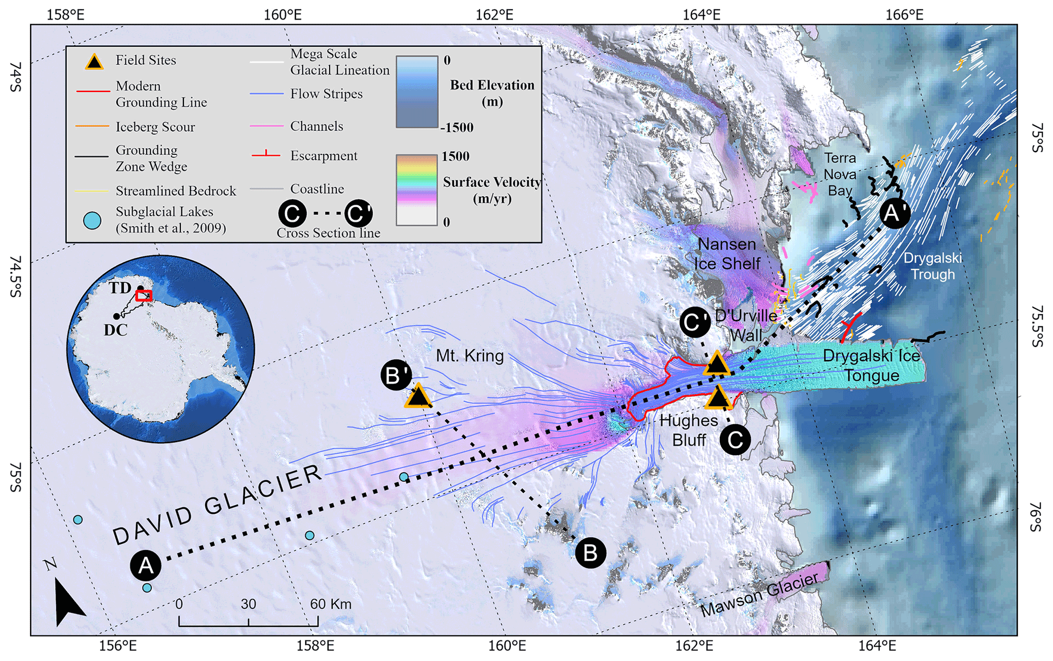
Figure 1Map of the greater David Glacier/Terra Nova Bay region including mapped submarine geomorphic features and geographic features mentioned in text. Geomorphic cross sections (A–A’, B–B’ and C–C’) highlighted in Fig. S1. Inset shows extent of main map along with drainage basin of David Glacier and position of two local ice domes: Dome C (DC) and Talos Dome (TD). Data sources: satellite imagery of Bindschadler et al. (2008), ice surface velocity of Rignot et al. (2011), surface elevation of Howat et al. (2019), bed elevation of Fretwell et al. (2013) and bathymetry of Arndt et al. (2013)
Geological reconstruction of the Antarctic Ice Sheet (AIS) through time provides critical insights into the history of ice sheet change and can narrow uncertainty on Antarctica’s contribution to global sea-level rise. A geologic perspective on ice sheet behaviour is particularly useful due to the following.
-
Quantitative satellite observations only extend back ∼ 40 years (IMBIE, 2018; IPCC, 2013; Miles et al., 2013; Rignot et al., 2019), and these observations do not fully capture natural variability of ice sheet behaviour.
-
Integration of the data constraining marine extent and terrestrial thickness of an ice mass through time provides a robust data set for evaluation of numerical ice sheet model simulations, which are used to predict future ice sheet contributions to sea-level rise.
-
Recent studies of the complex interactions between the solid earth, cryosphere and ocean highlight the need to understand short- and long-term changes in the AIS (Barletta et al., 2018; Whitehouse et al., 2019; Meredith et al., 2019). Modern continuous GPS measurements of bedrock deformation record the integrated response to both modern and ancient ice mass change. The elastic component due to modern ice mass fluctuations can be modelled using satellite observations constraining ice mass balance. The viscous component represents a “memory” of ice load history over centuries to millennia. Ice load reconstructions constrained by cosmogenic dating of glacial samples provide a powerful tool to robustly model glacial isostatic adjustment (GIA), a complex suite of ice-sheet–bedrock–sea-level feedbacks critical for projections of future global sea level.
Reconstructions of marine-terminating outlet glaciers provide an opportunity to constrain and understand the terrestrial and marine sectors of ice sheets. At the LGM, the David Glacier thickened and expanded as an ice stream, coalesced with grounded marine-based ice and extended hundreds of kilometres into the western Ross Sea (Anderson et al., 2014; Livingstone et al., 2012; Shipp et al., 1999). During deglaciation, grounding-line retreat from north of Coulman Island was initiated by ∼ 13 ka, and by 11 ka, the grounding line had retreated near the Terra Nova Bay (TNB) region (Licht et al., 1996; Domack et al., 1999a; McKay et al., 2008; Anderson et al., 2014; Yokoyama et al., 2016). By ∼ 10 ka, 14C dating of acid insoluble organic (AIO) matter from sediment cores suggests the grounding line in the Ross Sea had migrated south of the David Glacier (Licht and Andrews, 2002). However, AIO dates in the Ross Sea are known to be unreliable due to potential input of anomalously old carbon by reworking, and this 10 ka constraint is likely to represent a maximum age of this retreat (Andrews et al., 1999; Rosenheim et al., 2013). Marine sedimentary cores from the deepest parts of the inner Drygalski Trough provide evidence of a lingering ice shelf, but anomalously old surface 14C ages mean that the timing of this ice shelf presence is uncertain (Licht et al., 1996; Frignani et al., 1998; Domack et al., 1999a; Licht and Andrews, 2002; Prothro et al., 2020). North of TNB, meteoric 10Be and compound-specific radiocarbon ages capture the retreating calving line and onset of open marine conditions by 8 ka (Yokoyama et al., 2016). Grounding-line retreat north of Ross Island was achieved by ∼ 8.6 ka, and a modern configuration was established by ∼ 2–4 ka (Anderson et al., 2014; McKay et al., 2016).
Outlet (Reeves and Priestley glaciers) and valley glaciers (Tucker and Campbell glaciers) along the northern Victoria Land sector began thinning at ∼ 17 ka, and the majority of thinning ceased by ∼ 7.5 ka, broadly coincident with a linear rise in sea level and ocean temperatures throughout deglaciation (Baroni and Hall, 2004; Johnson et al., 2008; Smellie et al., 2018; Goehring et al., 2019; Rhee et al., 2019). In contrast, outlet glaciers covering a large swath of the TAM from Southern Victoria Land to Southern TAM experienced episodic thinning during the early-mid Holocene, likely due to local topographic effects associated with marine ice sheet instability (Jones et al., 2015; Spector et al., 2017). Along the Transantarctic Mountains, mid-Holocene outlet glacier thinning and retreat occurred during a relatively stable period of air temperature and sea level after the majority of post-glacial sea-level rise and rising atmospheric temperatures occurred (Lambeck et al., 2014; Jones et al., 2015; Spector et al., 2017; Jones et al., 2020). Overall, variation in the timing of glacier thinning suggests sea-level rise, ocean warming and overdeepened subglacial topography controlled the reconstructed glacier behaviour.
Surface exposure dating using in situ terrestrial cosmogenic nuclides has transformed the ability to reconstruct the AIS through time (e.g. Stone et al., 2003; Mackintosh et al., 2007; Todd et al., 2010; Balco, 2011; White et al., 2011; Jones et al., 2015; Spector et al., 2017; Small et al., 2019). Through surface exposure dating of glacial deposits, this study aims to constrain the LGM to present behaviour of the David Glacier. Guided by our resulting ice thinning histories, we investigate the forcings and controls on glacier thinning using a glacier flowline model. We use geologic data and ice sheet model outputs to frame and inform the first detailed deglacial sensitivity experiments for David Glacier, building on previous flowline modelling approaches in Antarctica (Jamieson et al., 2012; Jones et al., 2015; Whitehouse et al., 2017).
2.1 Field and laboratory methods
Glacial erratics and glacially striated bedrock were collected adjacent to the David Glacier both upstream and downstream of the present-day grounding line. Downstream sites, Hughes Bluff and D'Urville Wall, are expected to show the most recent and dramatic changes in ice thickness, while smaller and longer-term changes are expected at the upstream site, Mt Kring. (Fig. 1) (Anderson et al., 2004; Bockheim et al., 1989). Using the structure-from-motion photogrammetry technique (Vargo et al., 2017), we use helicopter-based photography to construct a high-resolution digital elevation model of each field site, allowing integration of glacial geological field surveys with the regional and local geomorphology (Baroni et al., 2004) (Figs. S3 and S4).
We primarily sampled glacial erratic cobbles from local glacial deposits and glacially moulded bedrock surfaces along vertical transects perpendicular to the modern glacial flow direction. The cosmogenic nuclide inventories in cobbles and bedrock comprise signals of both exposure since the most recent deglaciation and nuclides accumulated during any prior exposure (known as “inheritance”). For long-lived nuclides such as 10Be, this inherited component can be significant (Sugden et al., 2005; Balco, 2011). Inheritance of cosmogenic nuclides is widespread in Antarctica as the cold-based nature of some ice acts to cover (preventing build-up of cosmogenic nuclides) without causing significant erosion (Sugden et al., 2005; Atkins, 2013). However, since cosmic rays attenuate rapidly with depth into rock, subglacial erosion of more than a few metres can reset the cosmic-ray signal. As such, we primarily focused on sampling faceted and striated glacial erratics because they indicate a subglacial origin which reduces the likelihood of a prior exposure history, and these intact features indicate minimal post-depositional erosion. Exposure ages from these samples are interpreted to track glacier thinning at the site because such samples would have been brought to the glacier surface by upward-flowing ice before being deposited at the ice margin (Stone et al., 2003; Mackintosh et al., 2007; Fogwill et al., 2012; Jones et al., 2015; Small et al., 2019).
We use cosmogenic nuclides 10Be and 3He to determine surface exposure ages on 45 samples. For 10Be analysis, quartz is the target mineral and is present in granites and sandstones. For 3He, pyroxene is the target mineral and present in dolerites. In the field, we preferentially sampled on isolated, local topographic high points, distant from areas of blue ice, snow drifts or local till deposits. While it is the focus of this study to use glacial erratics to track glacier thinning, we also collected bedrock samples to better understand complex exposure histories due to burial and the non-erosive nature of cold-based ice (Atkins, 2013; Joy et al., 2014).
Samples were processed at the cosmogenic nuclide facilities at Te Herenga Waka Victoria University of Wellington. For 10Be, we separated quartz by crushing and sieving to extract the 250–500 mum grain size fraction. Magnetic minerals were separated using a Frantz isodynamic magnetic separator. For granitic rocks, feldspars were removed by froth flotation. We etched samples for 1 d in 10 % hydrochloric acid, for 1 d in 2.5 % hydrofluoric acid (HF) and for 3 d in 1 % HF to further purify the quartz separates. Beryllium was extracted from quartz following an established method including the addition of a 9Be carrier, enhanced quartz etching and digestion followed by ion exchange chromatography and BeOH precipitation (Norton et al., 2008). Targets of BeO were packed and sent to the Purdue Rare Isotope Measurement Laboratory (PRIME lab) for analysis using accelerated mass spectroscopy (AMS). For 3He, we targeted pyroxene from the 125–250 mum grain size fraction. Pure pyroxene was obtained using an established HF etching method, and 3He 4He ratios were measured at the Berkeley Geochronology Center noble gas spectrometer (Bromley et al., 2014; Blard et al., 2015; Balter-Kennedy et al., 2020). We supplemented this data set with eight samples collected prior to the 2016–2017 austral summer, and those samples were processed for10Be or 3He using methods outlined in Oberholzer et al. (2003, 2008) and Di Nicola et al. (2009, 2012). Exposure ages are calculated by converting the AMS-derived 10Be 9Be ratio to 10Be concentration by subtracting a known amount of 9Be carrier added during chemical processing. Final exposure ages are calculated using 10Be or 3He concentration, field information (elevation, shielding and sample thickness) and production rate scaling method (LSDn) (Balco et al., 2008; Lifton et al., 2014; Marrero et al., 2016; Jones et al., 2019). For 10Be, we employed Jones et al. (2019) systematics (http://ice-tea.org/en/, last access: 21 October 2021), and for 3He, we use Balco et al. (2008) systematics (https://hess.ess.washington.edu/, last access: 21 October 2021). All relevant data used to calculate exposure ages are served on the ICE-D online database (Balco, 2020) within the David Glacier region (http://antarctica.ice-d.org/, last access: 21 October 2021) and in Supplement Tables S1–S5. The resulting glacier thinning chronologies derived from surface exposure ages inform our glacier modelling approach by providing geometric targets for evaluating the simulated maximum thickness of ice and the subsequent magnitude and duration of glacier thinning.
2.2 Glacier modelling approach
To understand potential controls on grounding-line migration and onshore thinning, we apply a glacier flowline model to the David Glacier. Originally designed to track grounding-line migration using a moving grid, the flowline model we employ has been described fully elsewhere (e.g. Vieli and Payne, 2005; Nick et al., 2009; Jamieson et al., 2012; Enderlin et al., 2013; Jamieson et al., 2014; Clason et al., 2016; Whitehouse et al., 2017). The underlying theory and governing equations are outlined in Vieli and Payne (2005), and here we describe the components pertinent to our research questions.
Our glacier modelling focuses on a ∼ 1600 km long flowline from Dome C to the western Ross Sea shelf edge. The domain consists of varying flow regimes and extends to areas where the ice stream converged with grounded ice in the western Ross Embayment during the LGM. Ice flow is governed by fundamental Eqs. (1)–(6).
Ice flow along the grounded portion of the model domain, u, is calculated using the shallow ice approximation, which assumes ice flow only from internal ice deformation and horizontal velocity defined as
where n(=3) is Glen's flow law exponent, s is ice surface elevation, H is ice thickness and C is a constant given by
where A is the temperature-dependent rate factor (for −20 ∘C), ρi is ice density (0.910 g/cm3) and g is gravitational acceleration (9.8 m/s2).
As ice reaches flotation, ice is assumed to spread unidirectionally along the flowline, and ice flow is balanced by
where and v is the vertically average effective viscosity defined as
where is the effective strain rate.
For an ice stream, Eq. (3) is modified by including a basal traction coefficient β which is linearly related to the horizontal velocity u and is given by
We also incorporate a width term, including flat, a lateral buttressing factor, to account for lateral buttressing along a coupled ice stream shelf. Thus, as in previous applications of this model (Nick et al., 2010; Jamieson et al., 2012; Whitehouse et al., 2017) the final ice thickness (h) and width (W) averaged ice flow (u) is computed using the following equation:
flat controls the strength of lateral drag exerted at the ice stream margins. For all experiments in this study, flat is only altered where the ice stream is floating. When flat equals 1, full effects of lateral drag are felt; when values of flat are greater than 1, the magnitude of buttressing applied to the margins of the ice stream is reduced non-linearly.
The inclusion of the width term allows modelling of changing offshore trough width, which is common in palaeo-ice streams and outlet glaciers and is further supported by geomorphic interpretations using high-resolution bathymetry data (Jamieson et al., 2012; Livingstone et al., 2012, 2016). To determine offshore trough width, we map all glacial geomorphic features using the global multi-resolution topography data set within GeoMapApp (http://www.geomapapp.org, last access: 21 October 2021) based on analogues (Dowdeswell et al., 2016) and prior regional mapping (Stutz, 2012; Shipp et al., 1999; Anderson et al., 2014; Halberstadt et al., 2016).
Whitehouse et al. (2017) improved the ice shelf dynamics to incorporate the treatment of large horizontal grounding-line movements that are expected for the palaeo-David Glacier based on the long-term presence of the Drygalski Ice Tongue and evidence of extensive sub-ice-shelf conditions inferred from marine sedimentary cores (Domack et al., 1999a; McKay et al., 2008). In the model, the ice shelf geometry evolves with time, and variations in ice shelf thickness and extent are fed into lateral drag calculations (Whitehouse et al., 2017). Improved treatment of ice shelf dynamics allows exploration of the grounding-line sensitivity to ice shelf feedbacks. Importantly for this study, a reduction in lateral buttressing from adjacent, coalesced ice is expected as the expanded David Glacier and grounded ice in the Ross Sea decouple, which has been suggested from interpretation of submarine geomorphic features in the western Ross Sea (Shipp et al., 1999; Halberstadt et al., 2016).
Accumulation in the model is applied using modelled modern rates at the central flowline and multiplied to account for the ice stream width (W). Accumulation is then scaled to represent warmer or cooler conditions in our experiments (see Sect. 2.2.2). Where an ice shelf is present, sub-ice-shelf melt rates (SIMRs) are applied as a linear function of the depth of the ice shelf draught. From a minimum rate of 0.1 m/yr at 0 m (the ocean surface), SIMR increases to a maximum value at a depth of 500 m, and where ice shelf draught is deeper than 500 m, the maximum value is applied.
2.2.1 Boundary conditions
The model domain, sampled at 5 km resolution, runs along a ∼ 1600 km flowline from Dome C to the continental shelf break (Figs. 2 and S6). Figures 1 and S1 provide map extent of cross section views detailing the subglacial topography surrounding the modern-day grounding line. To simplify the flowline domain, we focus on the dominant ice stream emanating from Dome C. Using standard basin delineation tools in ArcGIS, we construct a drainage basin outline from surface elevation and ice velocity (Rignot et al., 2011; Howat et al., 2019). We then construct a flowline that follows the centre of the ice stream and thereafter calculate ice stream width perpendicular to this flowline (W) to create a defined lateral ice stream margin across the entire domain. Following Jamieson et al. (2012), the lateral ice stream margins in the offshore parts of the domain are determined using geophysical data to map the distribution of trough parallel mega-scale glacial lineations (MSGLs) that are indicators of past ice stream flow and thus show the width of the ice stream. Onshore, the lateral margins are defined by the valley width. The ice stream width perpendicular to the flowline is thereafter used to control the lateral stress applied by coalesced ice along the flowline (Eq. 6).
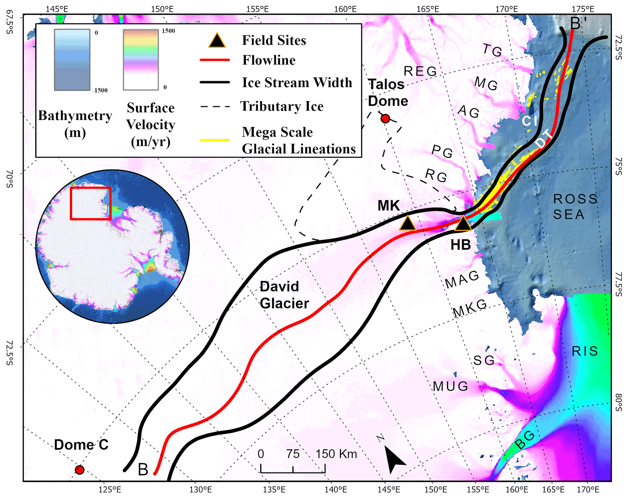
Figure 2Map of model domain with modern ice surface velocity of Rignot et al. (2011) and bathymetry of Arndt et al. (2013). Flowline follows red line; ice stream width in black. RIS: Ross Ice Shelf; BG: Byrd Glacier; MUG: Mulock Glacier; SG: Skelton Glacier; MKG: Mackay Glacier; MAG: Mawson Glacier; RG: Reeves Glacier; PG: Priestley Glacier; MG: Mariner Glacier; AG: Aviator Glacier; TG: Tucker Glacier; CI: Coulman Island; DT: Drygalski Trough; HB: Hughes Bluff; MK: Mt Kring.
To evaluate model performance and the appropriate boundary conditions for deglacial experiments, we tune basal traction (β), accumulation, sub-ice-shelf melt rate (SIMR) and rate factor (A) to reproduce the modern geometry and flow speed of the David Glacier as closely as possible. Modern ice surface elevation, surface mass balance and ice velocity are well constrained from satellite and in situ measurements (Rignot et al., 2011; van Wessem et al., 2018; Howat et al., 2019). We employ an ice mass accumulation scheme whereby tributary ice mass is added along the length of the ice stream (Jamieson et al., 2014; Whitehouse et al., 2017) to account for confluent ice from tributary glaciers. This tributary injection from a secondary ice stream originating from Talos Dome is included in the surface mass budget for the David Glacier model domain (Fig. 2).
Ongoing aerogeophysical and remote sensing techniques continue to reveal new detail of the subglacial environment of the AIS (Schroeder et al., 2020; MacGregor et al., 2021). Common among many TAM outlet glaciers, a prominent bedrock high immediately upstream of the modern grounding line provides a significant stabilising impact on the David Glacier (Fretwell et al., 2013; Morlighem et al., 2019). The bed geometry along the flowline is derived solely from Bedmap2 and the International Bathymetric Chart of the Southern Ocean (Fretwell et al., 2013; Arndt et al., 2013).
Geologic data from former glaciated terrains and satellite observations can be used to approximate basal conditions, yet a general lack of in situ data from the ice sheet basal environment leads to enduring uncertainties in the basal stress regime (Joughin et al., 2006; Stokes et al., 2015). Based on existing knowledge of sea floor morphology and consistent with previous modelling experiments, the basal traction parameter used in this model attempts a first-order approximation of two subglacial basal environments: (1) relatively high basal traction for onshore ice flow over bedrock and (2) relatively low basal traction for offshore ice flow over soft sediments associated with basal till deposits (Dowdeswell et al., 2004; O Cofaigh et al., 2005).
We use modelled surface mass balance (van Wessem et al., 2018), calculated SIMR (Wuite et al., 2009) and modern geometry (Howat et al., 2019; Fretwell et al., 2013) to set the model up so that it replicates modern flow conditions and geometry at a steady state (Table 1). We then tune the basal traction parameter to produce ice thickness and velocities which do not change significantly. The model is unable to reproduce stable conditions along the steep ice surface profile as the David Glacier descends from the ice sheet interior. In this zone, the modelled ice surface is steep and undergoes thinning throughout a 2000-year initiation period. In an effort to stabilise the ice surface upstream of the grounding line, we tune the basal traction parameter, effectively stiffening the bed, to reduce the modelled instability. We note here that according to Eq. (5), as the ice surface evolves, basal traction evolves naturally; for example, as the ice profile gets steeper or thicker, the basal traction evolves. Resultant modelled estimates of basal shear stress approach 100 kPa in this setting. While difficult to constrain with in situ measurements, Zoet et al. (2012) suggest higher stresses, such as these, should be expected near the modern-day grounding zone, which is consistent with the modelled stress distribution in this study. Overall, the modern grounding-line position, ice shelf thickness and ice shelf length do not vary significantly over a 2000-year modelled initiation period.
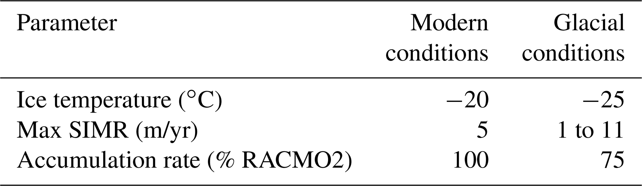
Table 1Parameter values used for sensitivity experiments indicating choices for model tuning to modern conditions over a spin-up period. Glacial conditions are parameter values used to simulate deglaciation. SIMR: sub-ice-shelf melt rate. Accumulation values reported as percentage of RACMO2 (van Wessem et al., 2018).
2.2.2 Deglaciation approach
LGM geometric boundary conditions incorporate modelled ice thickness and surface velocity from W12, an ice sheet reconstruction based on available geologic data (Fig. S6) (Whitehouse et al., 2012). Our ice flow model does not adjust for isostatic deformation as it evolves. Therefore, we use the W12 modelled ice thickness and modern bed elevation (Fretwell et al., 2013), which allows for a calculated estimate of upper ice surface without introducing uncertainty involving variable along-flow isostatic response and dynamic topography associated with the long-term evolution of the Antarctic subglacial topography (Stern et al., 2005; Whitehouse et al., 2019; Paxman et al., 2019). We do not compare our sensitivity experiment's results with those of the W12 ice reconstruction; we purely use a calculated upper ice surface as a starting point for our model during spin-up. The resulting ice thickness geometrically fits to geologic data (i.e. covers highest-elevation Holocene aged erratics) and serves as an initial ice profile for deglaciation sensitivity experiments.
To account for environmental changes during deglaciation, accumulation and internal ice temperature are tuned over the initial 7500 model years to ensure an LGM configuration that is consistent with geological constraints and has a grounding line that does not move significantly. Knowledge of past accumulation over glacial–interglacial cycles is restricted to ice core data and internal ice sheet layer mapping near high-elevation ice domes (Siegert, 2003; Frezzotti et al., 2005; Buiron et al., 2011; Cavitte et al., 2018). Generally, modern accumulation patterns show relatively low accumulation (0.02 m/yr) over the East Antarctic interior and high accumulation (0.2 m/yr) near the coastline (Arthern et al., 2006; Lenaerts et al., 2012; van Wessem et al., 2018). Interpretations from ice core records suggest LGM accumulation rates were lower than modern accumulation rates and generally correlate well with temperature proxy records throughout the Holocene (Siegert, 2003; Veres et al., 2013). We use a scaling relationship between modern and palaeo-accumulation patterns and estimate that accumulation at the start of the model run was roughly 75 % of modern accumulation (Veres et al., 2013). Internal ice temperature is increased through time to represent the increase in temperature that occurred during deglaciation. The internal ice temperature during deglaciation is not known, and for this study, we used values of −25 ∘C for the first 7500 model years and −20 ∘C during the remaining 7500 model years as a way to represent an appropriate amount of warming in the ice column. Deglacial sensitivity experiments use a range of accumulation and internal ice temperature forcings representing the potential scale of change experienced through a deglaciation (Table 1), allowing exploration of the relative influence of lateral buttressing reduction (LBR) and sub-ice-shelf melt rates (SIMR) on glacier thinning and retreat.
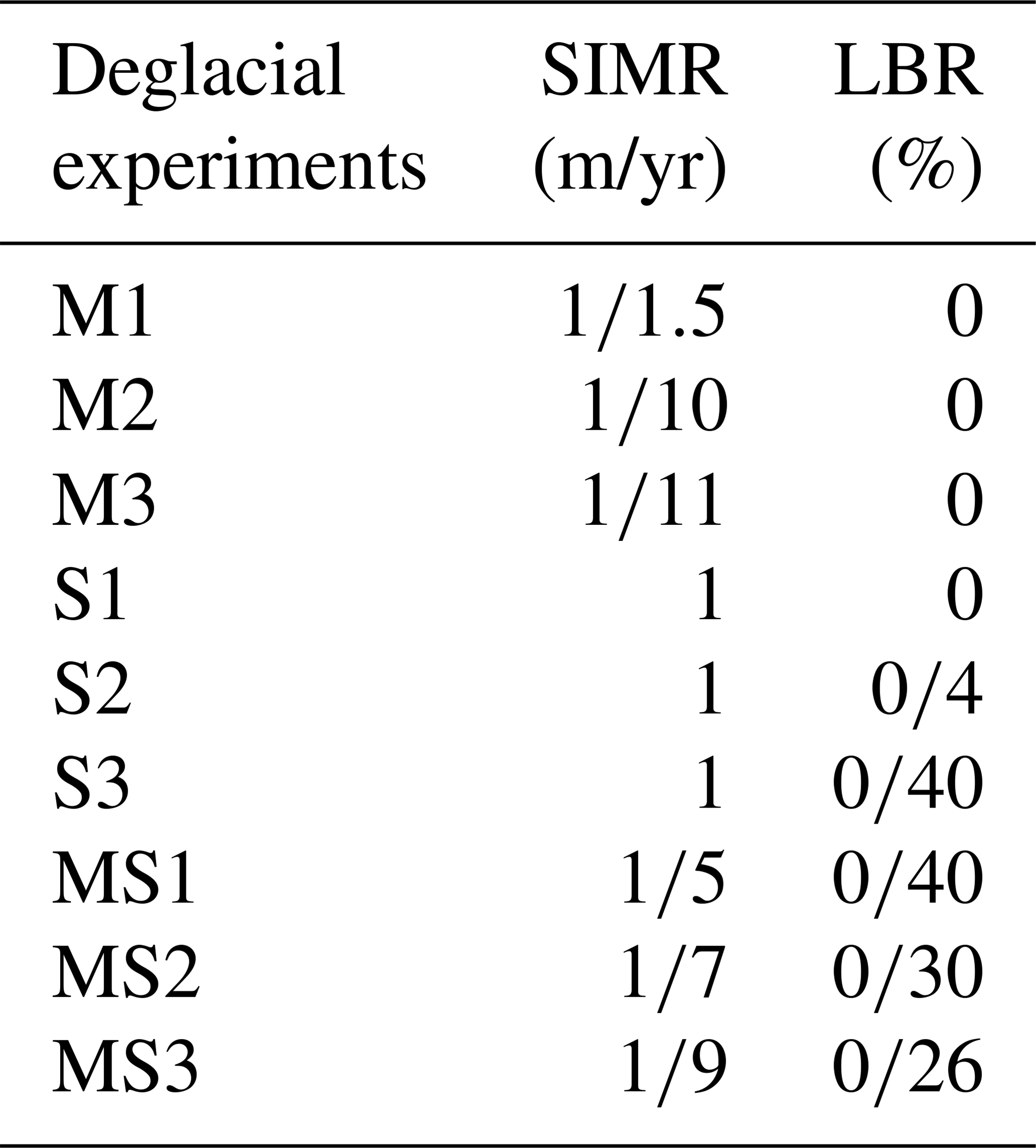
During the LGM, the David Glacier coalesced with grounded ice in the Ross Sea and was susceptible to ocean-driven basal melt and changes in lateral drag (buttressing) from surrounding grounded ice. We therefore run a suite of individual experiments that allow us to initiate grounding-line retreat by either linearly increasing SIMR or decreasing lateral buttressing over a 500-year period, with each model run applying different perturbed values for SIMR or LBR (Table 2). For combined forcing experiments (MS1–3), we alter both SIMR and LBR as above until the grounding-line retreats to a near modern configuration. We introduce a 1 kyr timing lag between SIMR forcing and LBR. This staggered forcing seeks to simulate ocean-driven melt occurring first followed by a reduction in lateral buttressing. This scenario is designed to represent a “calving bay” environment, potentially led by ocean-heat-driven sub-ice-shelf melt, as recognised in the western Ross Sea (Domack et al., 1999a, 2003, 2006) and East Antarctic margin (Leventer et al., 2006; Mackintosh et al., 2014).
All sensitivity experiments run for 15 kyr with an initial spin-up period lasting 7.5 kyr for SIMR forcing and 8.5 kyr for LBR forcing, at which point the forcing perturbation relating to increased SIMR or reduction in lateral buttressing is applied for the remaining modelled period. We run our experiments for 15 kyr to provide ample spin-up time at glacial conditions and force our model from 7.5 kyr to explore forcings that, by the end of the modelled period, result in a configuration consistent with modern observations. When forcing the model, we linearly increase the forcing over a 500-year period. To simulate the natural variability that might be expected in an ocean forcing record, we apply a fluctuation of up to 0.5 m/yr magnitude using a random noise generator, and this variation is then added on top of the 500-year increase in forcing that is already applied. Further, it is not the intention of these sensitivity experiments to reproduce the exact timing of marine-based grounding-line retreat along the David Glacier, but rather we aim to explore the range of possible drivers that would enable the overall scale of retreat observed between the LGM and present day. All idealised scenarios are presented in Table 2.
Table 2Idealised deglacial sensitivity experiments. Sub-ice-shelf melt rate (SIMR) varies within a 0.5 m/yr window around the value reported. SIMR is forced at 7500 model years, and lateral buttressing reduction (LBR) is forced at 8500 model years. X/Y indicates initial conditions and forced conditions, respectively. If held constant, one value is reported.
Of the 45 samples analysed in this study, 21 yield mid-Holocene exposure ages. Holocene aged samples are interpreted to have received minimal prior exposure (i.e. inheritance) and suggest a simple exposure history. Focusing on two sites, we derive a high-resolution chronology of glacier thinning from Mt Kring and Hughes Bluff.
3.1 Mt Kring
Mt Kring, situated in the interior of the EAIS, flanks the streaming ice of David Glacier draining Dome C. The nunatak, composed of layered dolerite, stands ∼ 300 m above the modern ice surface, henceforth “above the ice”. Of the 24 samples processed, 3 are dolerite bedrock and 21 are glacial erratics of mixed lithologies (Figs. 3 and S3). The bedrock surface at the peak of Mt Kring lacks glacial striations or erratics and has an apparent 3He bedrock exposure age of 554 ± 91 ka. A discontinuous, steep ridge line between ∼ 200–300 m above the ice was not sampled due to inaccessibility. At ∼ 200 m above the ice, the bedrock is striated parallel to the modern ice flow direction and has an apparent 3He exposure age of 550 ± 82 ka. The highest-elevation erratic is found at 171 m above the ice with increasing erratic abundance culminating in a drift sheet covering nearly all bedrock lower than ∼ 110 m above the ice. Striated, bulleted cobbles and boulders of dolerite, basalt and sandstone are common in the thin, patchy drift covering the bedrock. Based on our erratic exposure dating, the glacial drift here is a composite of three age populations (Fig. 4a). The younger population spans 7.4–5.5 ka (10Be, n=5) (Fig. 4b). An older population spans 51–25 ka (10Be, n=8 and 3He, n=4). The oldest erratic age population shows scattered evidence of glacial behaviour between 123–63 ka (10Be, n=2, 3He, n=2). The older populations are likely an artefact of repeated burial by overriding ice and multiple periods of exposure (i.e. inheritance).

Figure 3Orthomosaic map of Mt Kring with all exposure ages, 10Be (red) and 3He (grey), and total errors. Erratics and bedrock ages plotted as circles and squares, respectively. Bold ages indicate Holocene age erratics, and italicised ages indicate bedrock exposure. Large inset displays ice surface velocity of Rignot et al. (2011), and small inset displays LIMA data of Bindschadler et al. (2008). DG: David Glacier; DIT: Drygalski Ice Tongue; TNB: Terra Nova Bay; MK: Mt Kring.
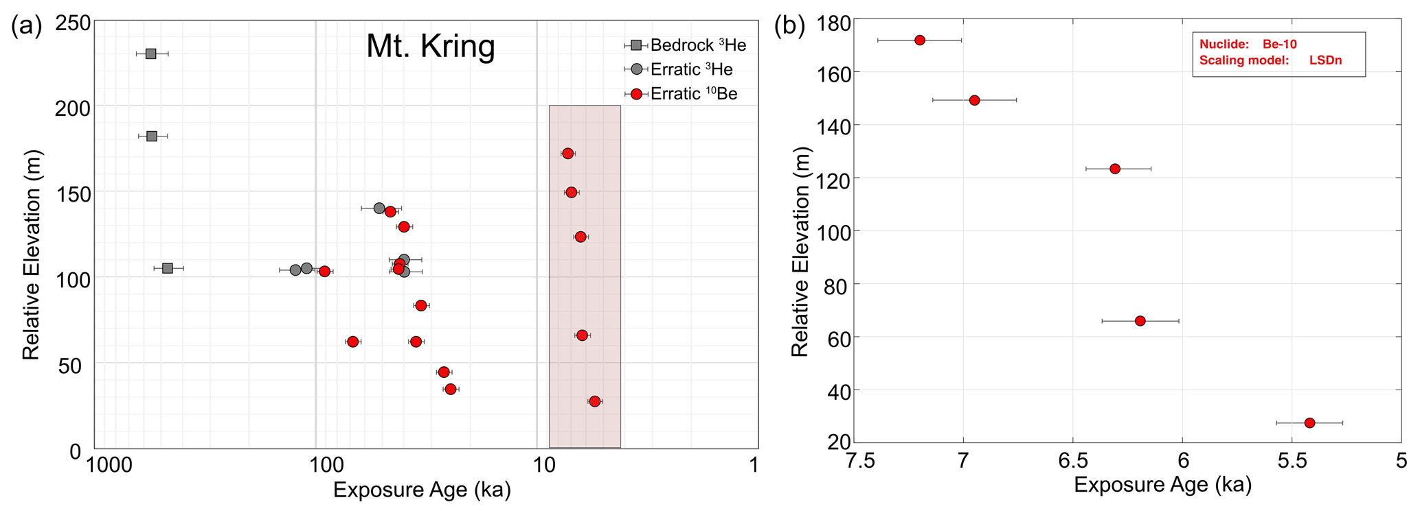
Figure 4Relative elevation, above the ice, vs. calculated surface exposure ages for Mt Kring. (a) All exposure ages. Erratics plotted as circles, bedrock as squares(10Be, red, and 3He, grey). Errors bars show total uncertainty. Panel (b) shows only Holocene ages.
3.2 Hughes Bluff
Hughes Bluff, situated on the Scott Coast, is a granite outcrop along the southern flank of the David Glacier. The outcrop is glacially scoured exhibiting spectacular rochés moutonnées, crescentic gouge marks and striations parallel to modern flow directions (Figs. 5 and S4). Scattered glacial erratics blanket the entire outcrop. 10Be exposure ages from 15 erratics span 6.7–4.3 ka (Fig. 6). The majority of glacial erratics are dated to between 6.7 and 6.2 ka. Two bedrock surface exposure ages sampled from rochés moutonnées at the highest and lowest outcrops (20.55 ka ± 2.10, 5.5 ± 0.47 ka) suggest significant wet-based glacial erosion since the LGM. At 20 m above the ice, similar bedrock and erratic ages provide evidence of recent emergence of this low-lying outcrop since 5.5 ka. The fact that well-developed landforms of glacial erosion occur at the highest outcrops at Hughes Bluff, including evidence of abundant basal sliding and plucking, indicate that ice thickness during the LGM was considerably greater than 230 m, the maximum elevation at Hughes Bluff (Frisia et al., 2017). While the onset and magnitude of thinning prior to 6.7 ka is not constrained, the Hughes Bluff chronology clearly indicates a period of rapid ice surface lowering during the mid-Holocene.
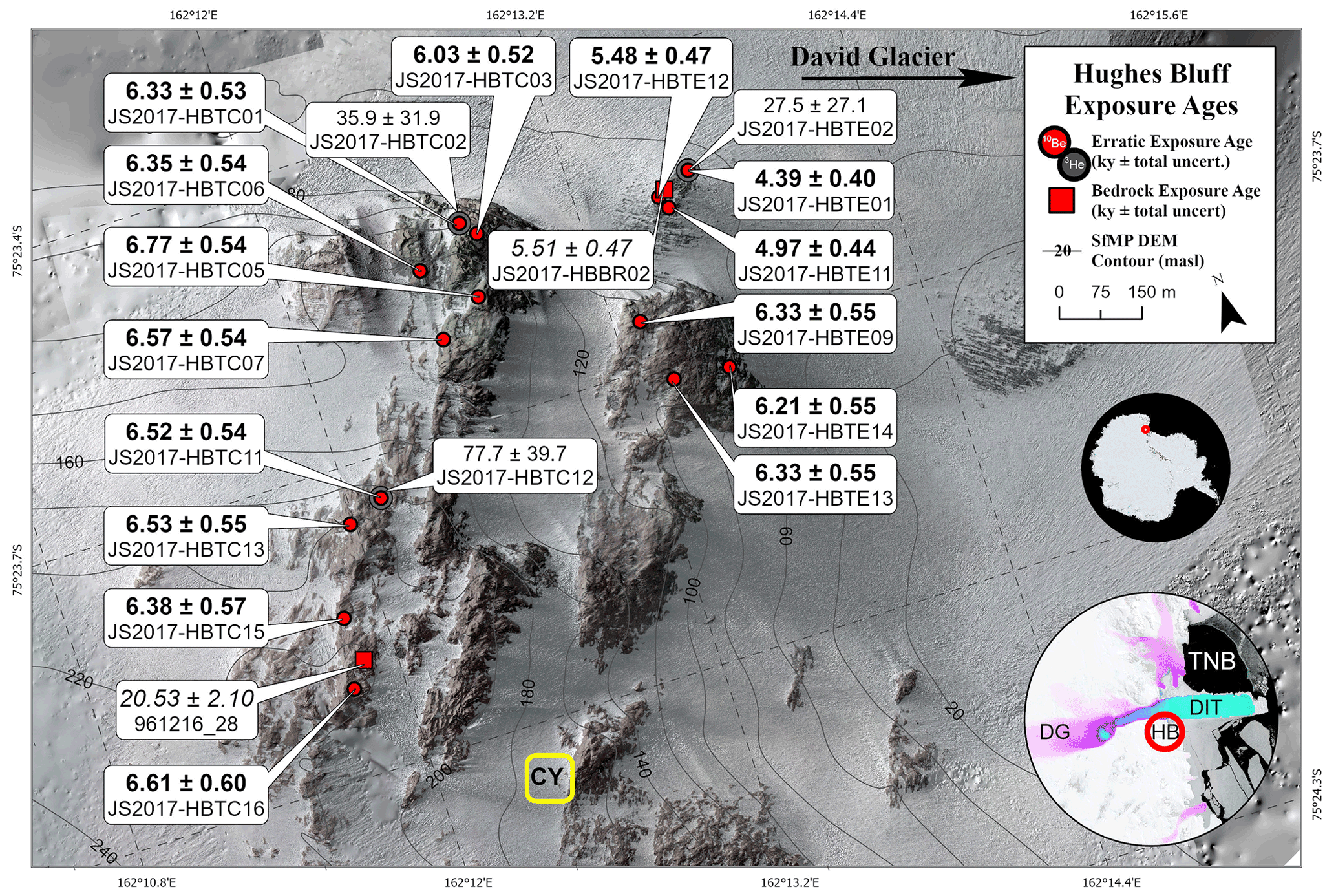
Figure 5Orthomosaic map of Hughes Bluff with all exposure ages, 10Be (red) and 3He (grey), and total errors listed. Erratics and bedrock ages plotted as circles and squares, respectively. Bold ages indicate Holocene age erratics, and italicised ages indicate bedrock exposure. Large inset shows ice surface velocity of Rignot et al. (2011), and small inset shows LIMA data of Bindschadler et al. (2008). DG: David Glacier; DIT: Drygalski Ice Tongue; TNB: Terra Nova Bay; HB: Hughes Bluff; CY: Camp Yellow.

Figure 6Relative elevation, above the ice, vs. calculated surface exposure ages for Hughes Bluff. (a) All exposure ages. Erratics plotted as circles and bedrock as squares (10Be, red, and 3He, grey). Errors bars show total uncertainty. Panel (b) shows only Holocene ages.
3.3 High-elevation constraints
In an effort to identify higher-elevation glacial activity and long-term erosion history, fieldwork was undertaken along the northern flank of David Glacier from the D'Urville Wall area (Mt Neumayer to Cape Phillipi) (Fig. S5). The D'Urville Wall is a steep, high-elevation (> 400 m above the ice) granite outcrop delimiting the northern flank of David Fjord. The geomorphology and exposure ages from two field sites situated high above the David Glacier (Mt Neumayer and Cape Phillipi) limit the reconstruction of the glacier surface during the LGM. Mt Neumayer extending above the D'Urville Wall forms a rounded summit with faint striations sub-parallel to modern ice flow and few scattered erratics (Baroni et al., 2004). In areas 400 m above the ice, bedrock samples contain weathering rinds and deep weathering pits filled with erratics (Baroni et al., 2004; Giorgetti and Baroni, 2007). Bedrock exposure ages from Mt Neumayer (649 m above the ice, 642 ± 61 ka), a terrace on top of the D'Urville Wall (418 above the ice, 116 ± 10 ka) and Cape Phillipi (∼ 300 m above the ice, 532 ± 52 and 957 ± 98 ka) suggest either a thin cover of cold-based ice or ice-free conditions through the LGM. Bedrock exposure ages from the D'Urville Wall area (including Mt Neumayer and Cape Phillipi) do not allow a precise estimate of the past ice surface along the northern flank of David Glacier. Supported by geomorphic evidence from Hughes Bluff, which indicates ice thicker than 230 m, and the LGM limit of ∼ 400 m a.s.l. derived from drift deposits in TNB, we suggest the past ice surface was between 300 and 649 m higher than today in this area (Stuiver et al., 1981; Orombelli et al., 1990; Di Nicola et al., 2009) (Fig. S2).
3.4 Palaeo-thinning rates
Using the high-resolution chronology from Hughes Bluff and Mt Kring, we derive a mean estimate of palaeo-thinning rates along David Glacier using a weighted least squares regression scheme within the iceTEA plotting tools (http://ice-tea.org/en/) (Jones et al., 2019). These reconstructed glacier thinning rates are compared to modern thinning rates derived from satellite data and continental-scale ice sheet models (Small et al., 2019). At Mt Kring, we reconstruct a 2 ka thinning event from 7.5–5.5 ka of up to 0.19 m/yr (0.06–0.19, 2σ) thinning rate (Fig. 7A). At Hughes Bluff, we reconstruct a period of rapid thinning from 6.7–6.2 ka of up to 2 m/yr (0.19–2.06 m/yr, 2σ) followed by ∼ 4 kyr period of minimal thinning (Fig. 7b). The reconstructed palaeo-thinning along the David Glacier during the mid-Holocene is synchronous with rapid thinning reconstructed at a number of sites in the Weddell embayment (Nichols et al., 2019; Johnson et al., 2019; Small et al., 2019; Bentley et al., 2017), Amundsen Sea sector (Johnson et al., 2008, 2014, 2017, 2020), Marie Byrd Land (Stone et al., 2003) and the Transantarctic Mountains (Todd et al., 2010; Jones et al., 2015; Spector et al., 2017; Jones et al., 2020). However, the rate of palaeo-thinning reconstructed at Hughes Bluff is one of the highest rates recorded in Antarctica, comparable to a reconstruction from nearby Mackay and Mawson glaciers (Small et al., 2019; Jones et al., 2015, 2020).
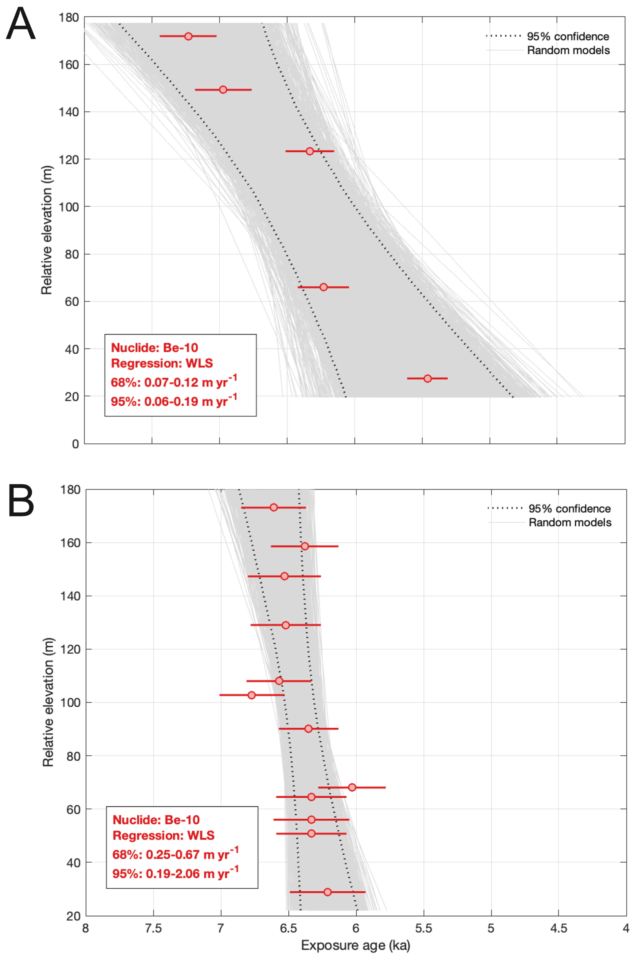
Figure 7Linear thinning rates derived from relative elevation, above the ice, and mid-Holocene exposure ages estimated using http://ice-tea.org/en/ from Jones et al. (2019) for (a) Mt Kring Holocene samples and (b) Hughes Bluff samples with outliers identified and omitted using outlier detection in http://ice-tea.org/en/.
Previous work from inland sites in a similar setting as Mt Kring suggested that such sites changed little or may have thickened during the Holocene due to accumulation increases (Bockheim et al., 1989; Denton et al., 1989). In contrast, the synchronous timing between thinning at Hughes Bluff and Mt Kring but lower thinning rate observed at Mt Kring suggests that this thinning event was driven by ocean–ice-sheet interactions at the coast that rapidly propagated inland. Such dynamic thinning, where increased ice shelf basal melting and grounding-line retreat leads to accelerated flow and inland thinning, is well documented along modern marine-terminating margins of the Greenland and Antarctic ice sheets (Pritchard et al., 2009, 2012), yet identification in the geologic record is rare, primarily due to a lack of exposed bedrock in the upper reaches of glacier catchments. The thinning history from David Glacier allows for a unique comparison with the broad pattern of dynamic thinning derived from the modern satellite record and suggests dynamic thinning can occur > 100 km into the interior of the EAIS and can persist over multiple millennia.
3.5 Exposure age data – ice sheet model comparison
During the LGM, ice core records and numerical model outputs suggest that the EAIS experienced widespread thinning in its interior, while coastal sites experienced extensive thickening (Verleyen et al., 2011; Mackintosh et al., 2014). Our data from Mt Kring show that the ice sheet was thicker than present at this site during the LGM and recorded at least 171 m of thinning during the Holocene. This provides a critical tie point between the high-elevation, low-accumulation ice domes where ice cores are drilled and the low-elevation, high-accumulation coastal sites with more abundant geologic data. Mt Kring is the first site along the high-elevation margin of the EAIS to constrain LGM ice sheet behaviour, and it represents a unique site to compare with other ice sheet reconstructions and continental-scale ice sheet modelling experiments.
The chronologies from David Glacier provide critical insights to the rate, timing, style and magnitude of thinning from a marine-based outlet glacier. The thinning histories presented here provide context to modelled continental-scale ice sheet reconstructions. Using a data–model comparison software, http://dmc.ice-d.org/, last access: 21 October 2021, we extracted a modelled elevation history for David Glacier from five different ice sheet models (four continental-scale and one regional-catchment scale) and one ice sheet reconstruction created to drive a GIA model (Argus et al., 2014; Pollard et al., 2016, 2017, 2018; Kingslake et al., 2018; Lowry et al., 2019). To overcome differences in spatial resolution, the scheme extracts an interpolated ice elevation history from the model grid cell containing the field site and its neighbouring model grid cells. The suite of ice sheet models in which we compare against our geologic data represent a variation in model grid size, flow approximations, model physics used, forcing and boundary conditions. We use them to provide a first-order approximation for expected results from the ice sheet modelling community.
The resulting data–model comparisons for Hughes Bluff and Mt Kring reveal a noticeable mismatch in time during the main phase of thinning (Fig. 8). For Mt Kring, ice sheet models indicate a phase of thinning that precedes our thinning history by ∼ 4–7 kyr. For Hughes Bluff, the timing lag is comparable to Mt Kring with one notable exception being the deglacial model of ICE-6G (Argus et al., 2014). This improved match is likely because ICE-6G is constrained by multiple relative-sea-level curves along the Scott Coast (Baroni and Hall, 2004; Hall, 2009; Argus et al., 2014). The style of thinning is variable between models with noticeable short-lived pauses in thinning, mainly during the Antarctic Cold Reversal (∼ 15–13 ka) (Pedro et al., 2016). Relative to Hughes Bluff, the magnitude of modelled elevation changes at Mt Kring geometrically fit better with the surface exposure age data. At Mt Kring, the average modelled thickness change throughout the deglacial phase for all models in Fig. 8a is 190 m ± 117 m, which compares well with the 173 m thickness change derived from our ice thinning chronology. In contrast, at Hughes Bluff, we capture only 171 m of thickness change over the deglacial period, and the average modelled thickness change for all models in Fig. 8b is 623 m ± 142 m. These comparisons suggest that our surface exposure ages capture more of the overall ice thinning at Mt Kring than at Hughes Bluff. Overall, the data–model mismatch may be related to (1) individual topographic features/outcrops not being spatially resolved in the models, (2) limited constraints on ocean/atmosphere forcing (e.g. Lowry et al., 2019) and (3) poorly constrained model parameters that influence basal sliding, isostatic adjustment and ice flow/rheology, which impact the rate of ice sheet response to a climate forcing (Lowry et al., 2020; Kingslake et al., 2018).
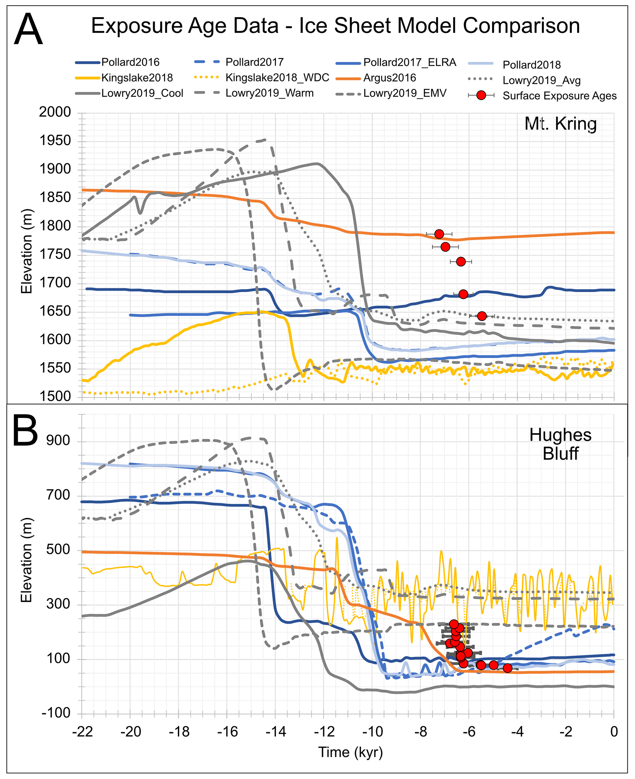
Figure 8Surface exposure age data – ice sheet model comparisons for (a) Mt Kring and (b) Hughes Bluff. Ice sheet modelled reconstruction data and supporting information from http://dmc.ice-d.org/ and Lowry et al. (2019). Kingslake2018_WDC uses WAIS Divide accumulation forcing, and Lowry2019_EMV is a model in which enhanced mantle viscosity is applied.
Based on the data-constrained thinning histories presented in this study, the main episode of glacier thinning occurred during the mid-Holocene and captures > 200 m of glacier change along the David Glacier. This time period does not correlate with significant increases in atmospheric temperature or global mean sea level (e.g. Lambeck et al., 2014; Menviel et al., 2011; Liu et al., 2009); therefore, we ask the following questions. (1) What is the role of ocean heat in driving the observed glacier thinning and retreat? And (2) given that ice from David Glacier coalesced with grounded ice in the Ross Sea during the LGM, what impact does ice sheet buttressing have on the timing and style of glacier thinning and retreat? The style and rate of modelled thinning and retreat from our flowline experiments are compiled in Table 3. We note we carried out many more experiments than reported here, and only those that show notable changes are presented. While we do not force our simulations by any date-specific reconstructions or proxy data, we co-view our model results against our geologic data to allow generalised time-varying geometric relationships to be compared.
Focusing solely on SIMR, a set of sensitivity experiments (M1–3) simulate the impacts of enhanced ocean heat on grounding-line retreat (Fig. 9). Modern SIMR have been calculated along the Drygalski Ice Tongue with an average of 4.89 m/yr ± 3.38 m/yr (Wuite et al., 2009). For our experiments, we progressively increased SIMR until retreat is initiated. Threshold values represent this stepwise increase in SIMR. After a 7.5 kyr spin-up period and for melt rates between 2 and 10 m/yr (represented by experiment M2), grounding-line retreat is initially rapid, but the final grounding line remains pinned to the prominent sill at the mouth of the David Fjord. A threshold SIMR of 11 m/yr achieves rapid grounding-line retreat behaviour and is consistent with the modern grounding-line position. Final modelled ice surface reconstructions for experiment M2 place the upper ice surface ∼ 300 m above the Hughes Bluff site. At Mt Kring, the final ice surface reconstruction for experiments M2 and M3 lies below the modern ice surface. In the high melt case (M3), the grounding-line position pauses at the sill for approximately 5 kyr. The final retreat phase from the sill to a modern position correlates with a final ice surface broadly consistent with modern observations.
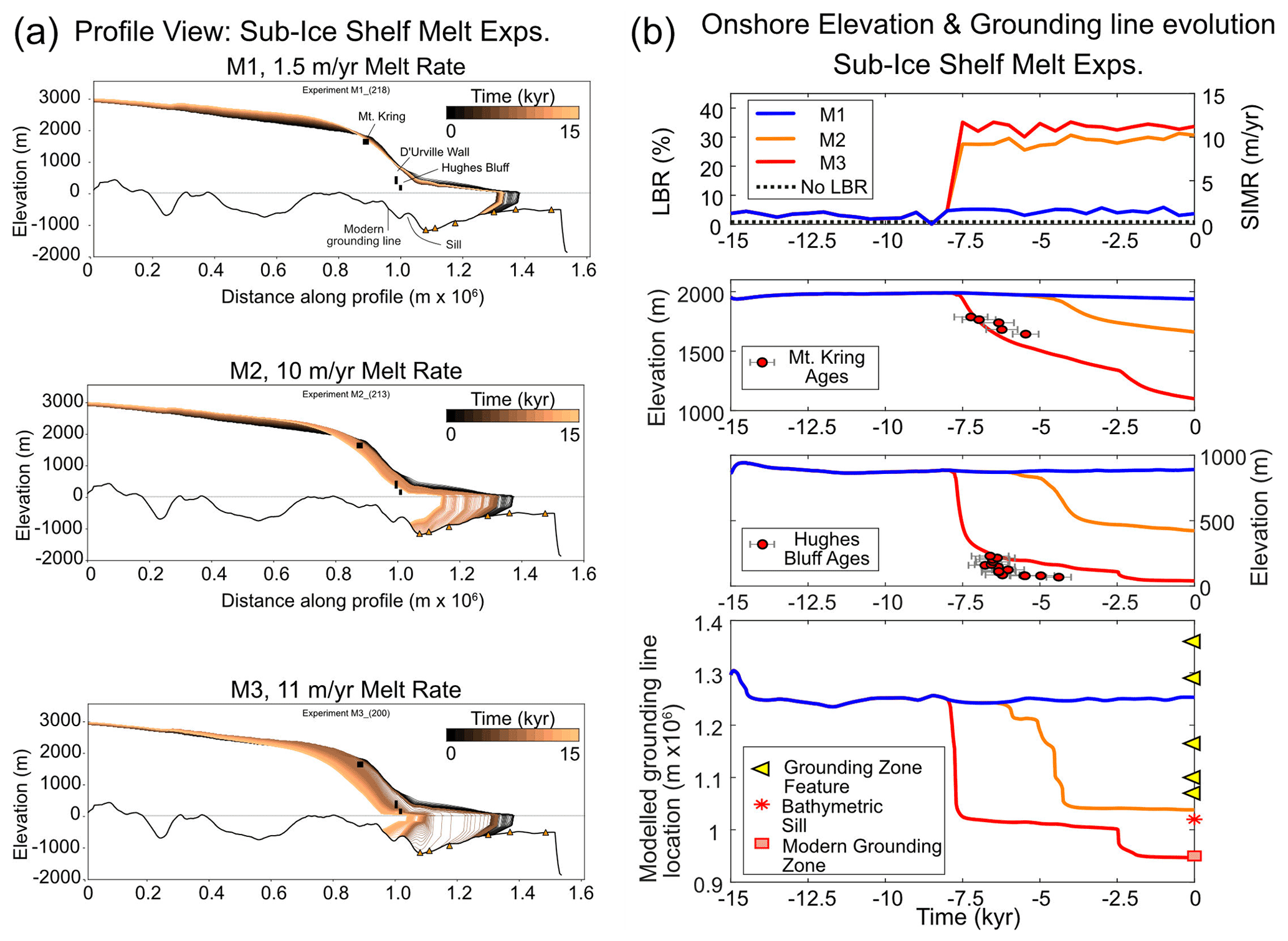
Figure 9(a) Profile view: 15 kyr evolution of modelled upper ice surface along flowline for sub-ice-shelf melt rate (SIMR) experiments. Black bars represent elevation range from three sites in this study. Orange triangles represent offshore features marking observed grounding zone wedges. (b) Onshore elevation and grounding-line evolution for SIMR experiments. Top subpanel: forcings applied (no relationship between LBR and SIMR). In SIMR cases, we varied the SIMR perturbation within a 0.5 m/yr window at 500-year temporal frequency to simulate short-lived pulses of relatively warmer or cooler water mass changes. Top middle subpanel: time-transgressive elevation profile for Mt Kring with exposure ages; bottom middle subpanel: time-transgressive elevation profile for Hughes Bluff surface exposure ages; and lower subpanel: evolution of grounding-line position with modern grounding-line position, bathymetric sill at the mouth of David Fjord and mapped grounding zone features. We co-view exposure age data in these plots to allow generalised time-varying geometric relationships to be compared.
Focusing on LBR experiments (S1–3), we simulate the impacts of glacier–ice-sheet decoupling on grounding-line retreat, a scenario suggested from glacial geomorphic features in the western Ross Sea (Shipp et al., 1999; Halberstadt et al., 2016) (Fig. 10). After a 8.5 kyr model spin-up period, ice shelf buttressing is incrementally reduced in successive simulations until retreat is initiated. Retreat occurs when lateral buttressing is reduced by 4 %. Ice shelf debuttressing by at least 40 % retreats the modelled grounding line to near-modern configuration, deep in the David Fjord. In both cases, the reduced buttressing forces rapid grounding-line retreat to a prominent sill at the mouth of the David Fjord. In these scenarios, the resulting modelled upper ice surface remains above the Hughes Bluff site when the grounding line is pinned to the sill. At Mt Kring, modelled rapid thinning is synchronous with Hughes Bluff, yet the 40 % LBR simulation (S3) results in an unrealistic final ice surface elevation hundreds of metres below the observed modern ice surface elevation.
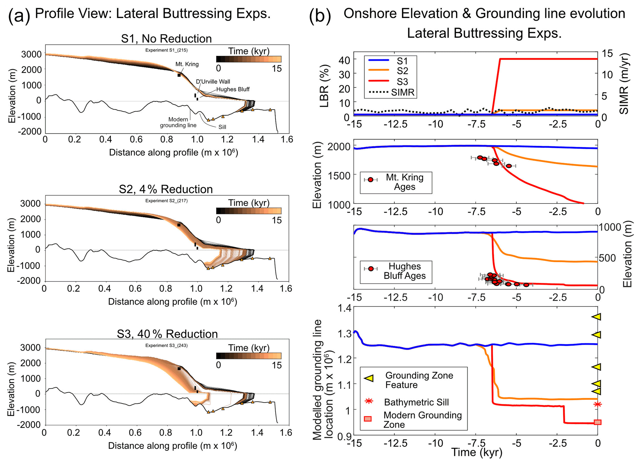
Figure 10(a) Profile view: 15 kyr evolution of modelled upper ice surface along flowline for lateral buttressing reduction (LBR) experiments. Black bars represent elevation range from three sites in this study. Orange triangles represent offshore features marking observed grounding zone wedges. (b) Onshore elevation and grounding-line evolution for LBR experiments. Top subpanel: forcings applied (no relationship between LBR and SIMR). Top middle subpanel: time-transgressive elevation profile for Mt Kring with exposure ages; bottom middle subpanel: time-transgressive elevation profile for Hughes Bluff surface exposure ages; and lower subpanel: evolution of grounding-line position with modern grounding-line position, bathymetric sill at the mouth of David Fjord and mapped grounding zone features. We co-view exposure age data in these plots to allow generalised time-varying geometric relationships to be compared.
Finally, we force our model with a combination of SIMR and LBR. Our approach is similar to that used for individual forcings, except that this time we use a melt rate (MS1: 5 m/yr) and progressively reduce lateral buttressing until the grounding line retreats to near-modern configuration. This approach is repeated for two additional cases of enhanced SIMR (MS2: 7 m/yr and MS3: 9 m/yr). Overall, when forcings are combined, lower threshold values are required to initiate thinning and retreat (Fig. 11). For experiments MS1–MS3, the final modelled upper ice surface reconstruction at Mt Kring lies below the modern ice surface. For experiments MS2–3, Hughes Bluff remains ice covered until grounding-line retreat from the sill approximately 5–6 kyr after the main phase of thinning and retreat.
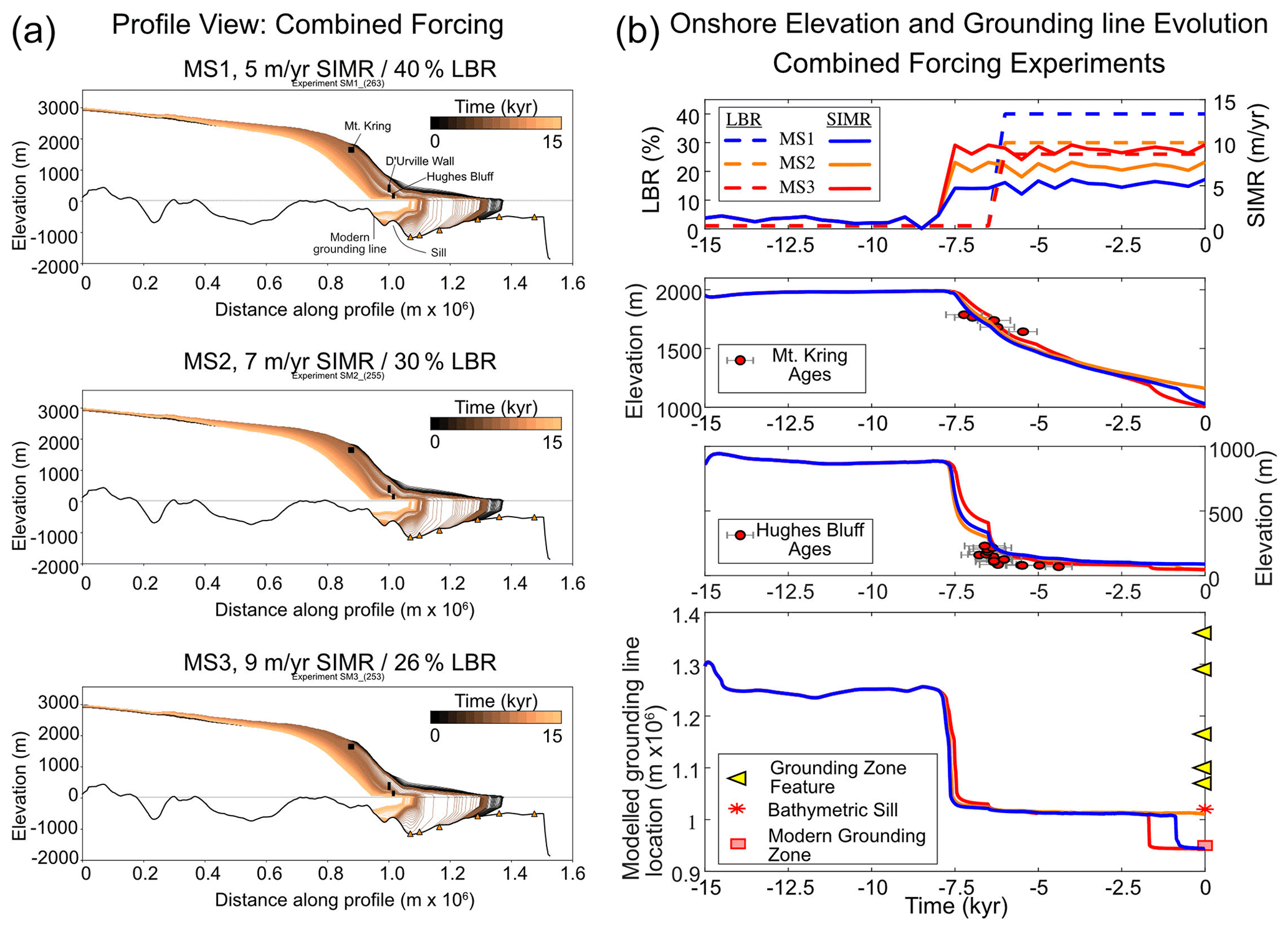
Figure 11(a) Profile view: 15 kyr evolution of modelled upper ice surface along flowline for combined forcing experiments. Black bars represent elevation range from three sites in this study. Orange triangles represent offshore features marking observed grounding zone wedges. (b) Onshore elevation and grounding-line evolution. Top subpanel: forcings applied (no relationship between LBR and SIMR). In SIMR cases, we varied the SIMR perturbation within a 0.5 m/yr window at 500-year temporal frequency to simulate short-lived pulses of relatively warmer or cooler water mass changes. Top middle subpanel: time-transgressive elevation profile for Mt Kring with exposure ages; bottom middle subpanel: time-transgressive elevation profile for Hughes Bluff surface exposure ages; and lower subpanel: evolution of grounding-line position with modern grounding-line position, bathymetric sill at the mouth of David Fjord and mapped grounding zone features. We co-view exposure age data in these plots to allow generalised time-varying geometric relationships to be compared.
We are confident that our modelling results reasonably reconstruct the period of multi-millennial glacial change during the mid-Holocene. However, our approach does have limitations including imperfect knowledge of past boundary conditions, treating ice as isothermal, lack of isostasy and subglacial hydrology parameterization, and no use of a calving law to control ice shelf length. Through modern sensitivity experiments, geologic control on geometry, and a general fit to modern SIMR and basal stress, we remain confident our results support a first-order approximation for the dominant controls on the David Glacier's thinning history.
Table 3Results for deglacial sensitivity experiments. We compare onshore and offshore modelled glacial behaviour, as well as thinning and grounding-line retreat rates. 1 Modelled retreat rate is calculated during the deglacial phase of experiments. 2 Data constrained maximum thinning rate at Mount Kring (MK) and Hughes Bluff (HB) is 0.19 and 2.06 m/yr, respectively. CI: Coulman Island.

The thinning history of David Glacier places modern observations in a long-term perspective and allows for local, regional and continent-wide comparisons with other glacial histories and modelled ice sheet reconstructions. High-resolution, low-inheritance exposure ages obtained from Hughes Bluff and Mt Kring overlap in time reveal different thinning styles with Hughes Bluff recording rapid ice surface lowering and Mt Kring revealing a much slower thinning signal. The chronology from Mt Kring implies glacier thinning reached far inland along zones of streaming ice and provides rare constraints on ice behaviour from the margins of the EAIS.
The results of flowline modelling experiments along the expanded David Glacier reveal a threshold-driven sensitivity to both SIMR and ice stream lateral buttressing. Combined forcing experiments show a similar rate and duration of onshore thinning compared with our onshore geologic records constrained by surface exposure studies at two locations along the flowline. The results show the glacier response occurs at lower threshold values when the processes act in combination, consistent with previous applications of this model (Jamieson et al., 2014). Although the sensitivity experiments do not resolve which process or combination of processes forced the observed onshore thinning, we discuss potential explanations for differences in our observed vs. modelled onshore glacier thinning.
5.1 Coastal thinning and impacts on local oceanography
Continental-scale ice sheet model reconstructions and available geological data suggest that the glacier thinning profile at Hughes Bluff likely only captures the final 200 m of the approximately 400+ m thinning since the LGM (Fig. S2). In total, marine geological evidence, ice modelling and new results in this study suggest that at the LGM the expanded David glacier had an ice surface profile above Hughes Bluff and a grounding-line location near Coulman Island (Licht et al., 1996; Domack et al., 1999a; Shipp et al., 1999; McKay et al., 2008). Flowline modelling experiments starting from this ice extent and thickness capture both the magnitude and rate of onshore thinning derived from surface exposure data.
The new geological reconstruction of ice surface elevation changes at Hughes Bluff shows a rapid lowering of the David Glacier at 6.5 ka and a period of slow thinning from ∼ 6–4 ka. Given the marked slowdown in thinning rate from ∼ 6 ka at Hughes Bluff and its location downstream of the present-day grounding line (Fig. 6b), we suggest that stabilisation of the Drygalski Ice Tongue occurred after ∼ 6 ka. This finding is consistent with Orombelli et al. (1990) and Baroni and Hall (2004), who mapped a series of raised beaches along the TNB coastline that mark beach depositional processes in an open ocean setting (i.e. no grounded ice) initiating at 7.2 ka. Stevens et al. (2017) show that the modern Drygalski Ice Tongue is essential for the development of the modern TNB polynya. Thus, if the Drygalski Ice Tongue formed at ∼ 6 ka as our exposure chronology from Hughes Bluff and the raised beach chronology from TNB suggest, it is likely that the TNB polynya has also existed since this time.
5.2 Palaeo-thinning rate comparison
General agreement between palaeo-thinning rates derived from surface exposure ages of glacial deposits and those from our modelling experiments provides confidence in the approach used in this study. In Table 3, we show that in the combined forcing experiments we achieve a close match between data-driven and glacier modelled thinning rates. For Hughes Bluff, a maximum thinning rate of 2.06 m/yr compares well with the average modelled thinning rate of 2.27 ± 0.29 m/yr (experiments MS1–3). At Mt Kring, the maximum thinning rate is 0.19 m/yr, and, for experiments MS1–3, the average modelled thinning rate is 0.36 m/yr ± 0.02 m/yr.
Our modelling demonstrates that glacier thinning at Mt Kring is sensitive to grounding-line migration during ice retreat from the outer to the inner continental shelf. Mt Kring is part of a broad bedrock platform along the northern flank of the major glacial trough dissecting the TAM (Fig. S1). The platform is comprised of three high-elevation outcrops protruding ∼ 200 m above the ice, with Mt Kring nearest to the zone of streaming ice (e.g. ice surface velocities > 100 m/yr). Geophysical characterisation of the northern TAM suggests the presence of individual tectonic blocks bounded by faults which likely serve as zones of relatively weak rock strength allowing preferential ice flow and glacial erosion (Salvini and Storti, 1999; Dubbini et al., 2010). In West Antarctica, dynamic thinning of the inland ice sheet has been linked to underlying tectonic controls (Bingham et al., 2012). At David Glacier, similar tectonic controls may have conditioned the spatial pattern of dynamic thinning during the Holocene.
Along the upper reaches of the David Fjord, there are no outcrops in the zone of highest ice surface velocity (> 100 m/yr). Mount Kring lies 40 km away from the modelled flowline, in an area of relatively slow flowing ice. Modern ice surface velocities near Mt Kring are ∼ 15 % of the ice surface velocities at the projected flowline position (Rignot et al., 2011). On modern ice sheets experiencing dynamic thinning, satellite-derived thinning estimates are largest in the centre of the ice streams or outlet glaciers and become progressively smaller at lower velocity sites further from the central flowline. For example, the central parts of Greenland’s outlet glaciers are currently thinning at rates of ∼ 0.84 m/yr, while marginal areas with slower ice velocities are thinning at 0.12 m/yr (Pritchard et al., 2009). Therefore, the Mt Kring site likely reflects ice stream marginal thinning (maximum of 0.19 m/yr, derived from surface exposure data) rather than the greater thinning rate that was experienced in the centre of an ice stream (modelled average maximum 0.36 m/yr ± 0.02 m/yr). Taken together, the Hughes Bluff and Mt Kring chronologies suggest that ∼ 2 kyr of dynamic thinning occurred at David Glacier and that this thinning propagated significantly into the ice sheet interior.
5.3 Controls on thinning and grounding-line migration
Overall, the style of modelled grounding-line retreat is controlled by marine ice sheet instability, a positive feedback where grounding-line retreat into overdeepened subglacial basins leads to progressively enhanced ice discharge and ice sheet thinning (Weertman et al., 1974; Mercer, 1978; Schoof, 2007). Experiments designed to simulate glacier–ice-sheet decoupling show that once independent, the David Glacier grounding line rapidly retreats through the Drygalski Trough and stabilises on a bathymetric sill at the mouth of the David Fjord.
This study provides insights into the processes that occurred as a large grounded section of an ice sheet retreated into discrete outlet glaciers. Previous descriptions of this retreat have focused on grounded ice in the Ross Sea as a whole (Licht et al., 1996; Shipp et al., 1999; Domack et al., 1999a; McKay et al., 2008; Anderson et al., 2014). However, at the scale of David Glacier, retreat was likely influenced by local processes including interactions with adjacent glaciers and other ice bodies. For example, a recent ice sheet retreat reconstruction of Halberstadt et al. (2016) suggests that ice lingered on higher-elevation banks as the grounding line retreated in adjacent, large bathymetric troughs. Modelled grounding-line retreat may have been slower in reality due to lateral buttressing from outlet glaciers on the TAM coast and stagnant ice on bathymetric highs immediately seaward of the expanded David Glacier, and such lingering ice is not accounted for in our simplified modelling approach.
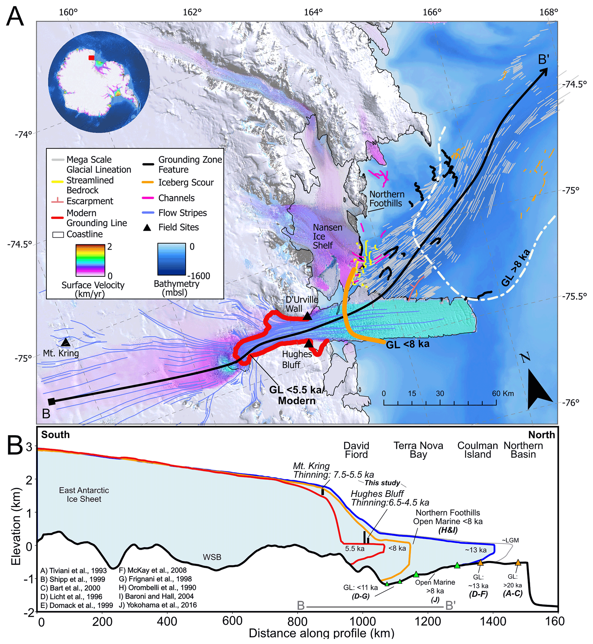
Figure 12(a) Map of David Glacier, Terra Nova Bay and surrounding areas. Synthesis map focused on two-phase retreat between > 8 and 5.5 ka, including geographic and geomorphic features mentioned in text. Ice surface velocity of Rignot et al. (2011) and LIMA satellite data of Bindschadler et al. (2008). Inset with red box for main extent shows bathymetry of Arndt et al. (2013) and ice surface velocity of Rignot et al. (2011). (b) Synthesis profile focused on two-phase retreat between 11 and 5.5 ka. Grounding zone features: triangles with age constraints (orange), triangles without age constraints (green) of Lee (2019). GL: grounding line.
Knowledge of this complex lingering ice history is poorly constrained as the majority of research has focused on trough axes (Anderson et al., 2014; Halberstadt et al., 2016), whereas offshore Mawson Glacier, south of David Glacier, submarine geomorphology reveals a complex record of lingering ice (Stutz, 2012; Greenwood et al., 2018; Prothro et al., 2020). Analysis of marine sediments, primarily from trough axes, indicates that a calving bay environment formed during grounding-line retreat (Domack et al., 1999a, 2003; Leventer et al., 2006; Mackintosh et al., 2014). In this scenario, grounding-line retreat is rapid along the trough axis, while lingering ice remains grounded along the lateral margins of the ice stream/glacier. In addition to sedimentary evidence, the abundant large iceberg keel marks seaward of the Coulman Island grounding zone wedge (GZW) and smaller keel marks within TNB provide evidence for a calving bay during deglaciation. Short-term grounding-line stagnation may have been facilitated by complex interaction with other outlet glaciers (Reeves and Priestley glaciers together forming proto-Nansen Ice Sheet/Shelf) of TNB or grounded ice lingering on the banks surrounding the Drygalski Trough, or both.
During the first ∼ 500 model years, the modelled grounding line initially retreats to the location of a large grounding zone wedge (Lee, 2019). A lack of modelled grounding-line stability at other, smaller GZWs suggests that the grounding line may only have experienced short pauses in these locations. Further, in the case of the much smaller GZWs observed in the deepest portion of the Drygalski Trough, the elongate morphology of these smaller GZWs may reflect a point source versus a line or zone source associated with more classically defined sheet-like GZWs. Regardless, the small mounds in the trough axis are likely to reflect short-lived grounding line pauses during overall retreat.
Generally, once initiated, the modelled David Glacier grounding line retreats rapidly and pauses at a prominent sill at the mouth of David Fjord for up to 5 kyr before subsequent grounding-line retreat to its modern configuration. This simulated two-phase grounding-line retreat aligns with phases of enhanced (at ∼ 6.5 ka) and reduced thinning (from 6 ka) identified in our onshore reconstructions at Mt Kring and Hughes Bluff, both in terms of timing and rates of past glacier thinning. Models forced by moderate SIMR and LBR (MS1–3) fit best with onshore geologic constraints.
Figure 12 synthesises the results of the terrestrial thinning chronology, modelled glacier flowline behaviour and the existing regional marine retreat chronologies. This synthesis suggests that beginning at 7.5 ka, the grounding line unpins from the sill at the mouth of the David Fjord, the David Glacier and proto-Nansen Ice Shelf decouple, and widespread onshore thinning is initiated. Between 6–5.5 ka, the grounding line retreats to near its modern position, thinning slows significantly and open marine conditions prevail regionally. In summary, geological evidence from offshore David Glacier indicates that retreat of grounded ice through the Drygalski Trough and the formation of open marine conditions similar to today occurred immediately prior to the dynamic thinning of David Glacier recorded in this study (Licht et al., 1996; Domack et al., 1999b; McKay et al., 2008; Yokoyama et al., 2016). Our onshore surface exposure data record the final stages of glacial thinning and retreat along the David Glacier.
Ice surface reconstructions from the David Glacier reveal a period of glacier thinning along a large swath of the drainage basin during the mid-Holocene (∼ 6.5 ka). The reconstructed thinning style between two sites separated by ∼ 130 km reveals a dynamic thinning event that endured for two millennia. This chronology is synchronous with local-, regional- and continental-scale geological records of ice sheet change yet is not fully captured in continental-scale ice sheet models. Our flowline modelling results suggest that thinning and grounding-line retreat were driven by increased sub-ice-shelf melt (SIMR) and decreased ice stream lateral buttressing and that the combination of these two processes reduces the individual forcing thresholds required to initiate retreat. Modelled patterns of grounding-line retreat correlate well with patterns of onshore thinning, constrained by our high-resolution surface exposure ages. Data–model mismatches likely highlight processes or feedbacks not represented in our simplified modelling approach related to the relative role of local topographic pinning points and the nature of ocean-forced dynamic thinning.
Through careful collection of glacial deposits from numerous sites along the David Glacier, we have improved the spatial and temporal resolution of the onshore reconstruction of the AIS. Our data constrain a 130 km portion of one of the largest outlet glaciers in the world which carries regional significance for Victoria Land and the western Ross Sea, as well as offering clues about processes currently underway in rapidly changing sectors of Antarctica and Greenland. While we acknowledge the data and modelling presented in this work may not apply to other settings, we hope that our study may serve as a template for future work aiming to extend the observations of ice sheet change beyond the last ∼ 40 years of satellite data.
The code used for flowline modelling is available by request from the corresponding author.
Field, lab, analytical and exposure age data are available on ICE-D online database (http://antarctica.ice-d.org/site/HUGBLUFF, Stutz et al., 2017a; http://antarctica.ice-d.org/site/DWALL, Stutz et al., 2017b; http://antarctica.ice-d.org/site/KRING, Stutz et al., 2017c; http://antarctica.ice-d.org/site/PHIL, Stutz et al., 2017d; http://antarctica.ice-d.org/site/MTNEU, Stutz et al., 2017e) and in Supplement Tables S1–S5.
Samples collected during the 2016/17 austral summer are curated at Te Herenga Waka Victoria University of Wellington and are available from the corresponding author. Samples collected prior to 2016/17 austral summer are curated at the University of Pisa.
The supplement related to this article is available online at: https://doi.org/10.5194/tc-15-5447-2021-supplement.
JS contributed to project design, fieldwork planning and implementation, sample analysis, modelling, and preparation of manuscript. AM contributed to original project design, fieldwork, modelling and manuscript preparation. KN contributed to original project design, sample analysis and manuscript preparation. RW contributed to field and lab work. CB and MCS led previous regional fieldwork, contributed data and helped prepare manuscript. SC contributed to field and lab work. SJ led modelling work and contributed to preparation of manuscript. RSJ contributed to project design and modelling work. GB contributed to project design and BGC-related lab work. PS contributed to data–model comparison (DMC) work. JL contributed unpublished bathymetry data and regional marine geologic observations. YBS contributed to regional synthesis discussion. TW, LD, MI, FS, SIO and MC conducted AMS analyses at respective laboratories. LV contributed through preparation of structure-from-motion photogrammetry (SfMP) models, modelling and manuscript preparation. DL contributed to DMC work. RM contributed to regional marine geology synthesis.
The authors declare that they have no conflict of interest.
Publisher’s note: Copernicus Publications remains neutral with regard to jurisdictional claims in published maps and institutional affiliations.
We would like to thank our trusty mountaineer Bia Boucinhas and pilot Mark Hayes for safe passage during fieldwork. Logistical support for fieldwork and lab work was expertly provided by Antarctica New Zealand; Italian National Antarctic Programme (PNRA); Korean Polar Research Institute (KOPRI); Southern Lakes Helicopters; Kenn Borek Air; Antarctic Research Centre; School of Geography, Earth and Environmental Studies; and Te Herenga Waka Victoria University of Wellington. We extend a great deal of gratitude for the many experienced researchers in the David Glacier area for providing field photos from past expeditions.
Field work, AMS analyses and a research visit to BGC was funded by NZARI (grant 2017-1-3). Antarctic Science Bursary provided funding for a research visit to Durham University. Andrew Mackintosh was supported by ARC SRIEAS grant SR200100005, Securing Antarctica’s Environmental Future.
This paper was edited by Pippa Whitehouse and reviewed by Keir Nichols and James Lea.
Anderson, B. M., Hindmarsh, R. C., and Lawson, W. J.: A modelling study of the response of Hatherton Glacier to Ross Ice Sheet grounding line retreat, Global Planet. Change, 42, 143–153, https://doi.org/10.1016/j.gloplacha.2003.11.006, 2004. a
Anderson, J. B., Conway, H., Bart, P. J., Witus, A. E., Greenwood, S. L., McKay, R. M., Hall, B. L., Ackert, R. P., Licht, K., Jakobsson, M., and Stone, J. O.: Ross Sea paleo-ice sheet drainage and deglacial history during and since the LGM, Quaternary Sci. Rev., 100, 31–54, https://doi.org/10.1016/j.quascirev.2013.08.020, 2014. a, b, c, d, e, f
Andrews, J. T., Domack, E. W., Cunningham, W. L., Leventer, A., Licht, K. J., Jull, A. J. T., DeMaster, D. J., and Jennings, A. E.: Problems and Possible Solutions Concerning Radiocarbon Dating of Surface Marine Sediments, Ross Sea, Antarctica, Quaternary Res., 52, 206–216, https://doi.org/10.1006/qres.1999.2047, 1999. a
Argus, D. F., Peltier, W. R., Drummond, R., and Moore, A. W.: The Antarctica component of postglacial rebound model ICE-6G_C (VM5a) based on GPS positioning, exposure age dating of ice thicknesses, and relative sea level histories, Geophys. J. Int., 198, 537–563, https://doi.org/10.1093/gji/ggu140, 2014. a, b, c
Arndt, J. E., Schenke, H. W., Jakobsson, M., Nitsche, F. O., Buys, G., Goleby, B., Rebesco, M., Bohoyo, F., Hong, J., Black, J., Greku, R., Udintsev, G., Barrios, F., Reynoso-Peralta, W., Taisei, M., and Wigley, R.: The International Bathymetric Chart of the Southern Ocean (IBCSO) Version 1.0-A new bathymetric compilation covering circum-Antarctic waters, Geophys. Res. Lett., 40, 3111–3117, https://doi.org/10.1002/grl.50413, 2013. a, b, c, d
Arthern, R. J., Winebrenner, D. P., and Vaughan, D. G.: Antarctic snow accumulation mapped using polarization of 4.3-cm wavelength microwave emission, J. Geophys. Res.-Atmos., 111, D06107, https://doi.org/10.1029/2004JD005667, 2006. a
Atkins, C. B.: Geomorphological evidence of cold-based glacier activity in South Victoria Land, Antarctica, Geological Society, London, Special Publications, 381, 299–318, https://doi.org/10.1144/SP381.18, 2013. a, b
Balco, G.: Contributions and unrealized potential contributions of cosmogenic-nuclide exposure dating to glacier chronology, 1990–2010, Quaternary Sci. Rev., 30, 3–27, https://doi.org/10.1016/j.quascirev.2010.11.003, 2011. a, b
Balco, G.: Technical note: A prototype transparent-middle-layer data management and analysis infrastructure for cosmogenic-nuclide exposure dating, Geochronology, 2, 169–175, https://doi.org/10.5194/gchron-2-169-2020, 2020. a
Balco, G., Stone, J. O., Lifton, N. A., and Dunai, T. J.: A complete and easily accessible means of calculating surface exposure ages or erosion rates from 10Be and 26Al measurements, Quat. Geochronol., 3, 174–195, https://doi.org/10.1016/J.QUAGEO.2007.12.001, 2008. a, b
Balter-Kennedy, A., Bromley, G., Balco, G., Thomas, H., and Jackson, M. S.: A 14.5-million-year record of East Antarctic Ice Sheet fluctuations from the central Transantarctic Mountains, constrained with cosmogenic 3He, 10Be, 21Ne, and 26Al, The Cryosphere, 14, 2647–2672, https://doi.org/10.5194/tc-14-2647-2020, 2020. a
Barletta, V. R., Bevis, M., Smith, B. E., Wilson, T., Brown, A., Bordoni, A., Willis, M., Khan, S. A., Rovira-Navarro, M., Dalziel, I., Smalley, R., Kendrick, E., Konfal, S., Caccamise, D. J., Aster, R. C., Nyblade, A., and Wiens, D. A.: Observed rapid bedrock uplift in Amundsen Sea Embayment promotes ice-sheet stability., Science, 360, 1335–1339, https://doi.org/10.1126/science.aao1447, 2018. a
Baroni, C. and Hall, B. L.: A new Holocene relative sea-level curve for Terra Nova Bay, Victoria Land, Antarctica, J. Quaternary Sci., 19, 377–396, https://doi.org/10.1002/jqs.825, 2004. a, b, c
Baroni, C., Frezzotti, M., Salvatore, M. C., Meneghel, M., Tabacco, I. E., Vittuari, L., Bondesan, A., Biasini, A., Cimbelli, A., and Orombelli, G.: Antarctic geomorphological and glaciological 1 : 250 000 map series: Mount Murchison quadrangle, northern Victoria Land. Explanatory notes, Ann. Glaciol., 39, 256–264, https://doi.org/10.3189/172756404781814131, 2004. a, b, c
Bentley, M., Hein, A., Sugden, D., Whitehouse, P., Shanks, R., Xu, S., and Freeman, S.: Deglacial history of the Pensacola Mountains, Antarctica from glacial geomorphology and cosmogenic nuclide surface exposure dating, Quaternary Sci. Rev., 158, 58–76, https://doi.org/10.1016/j.quascirev.2016.09.028, 2017. a
Bentley, M. J., O Cofaigh, C., Anderson, J. B., Conway, H., Davies, B., Graham, A. G., Hillenbrand, C.-D., Hodgson, D. A., Jamieson, S. S., Larter, R. D., Mackintosh, A., Smith, J. A., Verleyen, E., Ackert, R. P., Bart, P. J., Berg, S., Brunstein, D., Canals, M., Colhoun, E. A., Crosta, X., Dickens, W. A., Domack, E., Dowdeswell, J. A., Dunbar, R., Ehrmann, W., Evans, J., Favier, V., Fink, D., Fogwill, C. J., Glasser, N. F., Gohl, K., Golledge, N. R., Goodwin, I., Gore, D. B., Greenwood, S. L., Hall, B. L., Hall, K., Hedding, D. W., Hein, A. S., Hocking, E. P., Jakobsson, M., Johnson, J. S., Jomelli, V., Jones, R. S., Klages, J. P., Kristoffersen, Y., Kuhn, G., Leventer, A., Licht, K., Lilly, K., Lindow, J., Livingstone, S. J., Massé, G., McGlone, M. S., McKay, R. M., Melles, M., Miura, H., Mulvaney, R., Nel, W., Nitsche, F. O., O'Brien, P. E., Post, A. L., Roberts, S. J., Saunders, K. M., Selkirk, P. M., Simms, A. R., Spiegel, C., Stolldorf, T. D., Sugden, D. E., van der Putten, N., van Ommen, T., Verfaillie, D., Vyverman, W., Wagner, B., White, D. A., Witus, A. E., and Zwartz, D.: A community-based geological reconstruction of Antarctic Ice Sheet deglaciation since the Last Glacial Maximum, Quaternary Sci. Rev., 100, 1–9, https://doi.org/10.1016/j.quascirev.2014.06.025, 2014. a, b
Bindschadler, R., Vornberger, P., Fleming, A., Fox, A., Mullins, J., Binnie, D., Paulsen, S., Granneman, B., and Gorodetsky, D.: The Landsat Image Mosaic of Antarctica, Remote Sens. Environ., 112, 4214–4226, https://doi.org/10.1016/j.rse.2008.07.006, 2008. a, b, c, d
Bingham, R. G., Ferraccioli, F., King, E. C., Larter, R. D., Pritchard, H. D., Smith, A. M., and Vaughan, D. G.: Inland thinning of West Antarctic Ice Sheet steered along subglacial rifts, Nature, 487, 468–471, https://doi.org/10.1038/nature11292, 2012. a
Blard, P.-H., Balco, G., Burnard, P., Farley, K., Fenton, C., Friedrich, R., Jull, A., Niedermann, S., Pik, R., Schaefer, J., Scott, E., Shuster, D., Stuart, F., Stute, M., Tibari, B., Winckler, G., and Zimmermann, L.: An inter-laboratory comparison of cosmogenic 3He and radiogenic 4He in the CRONUS-P pyroxene standard, Quat. Geochronol., 26, 11–19, https://doi.org/10.1016/j.quageo.2014.08.004, 2015. a
Bockheim, J. G., Wilson, S. C., Denton, G. H., Andersen, B. G. B. G., and Stuiver, M.: Late Quaternary ice-surface fluctuations of Hatherton Glacier, Transantarctic Mountains, Quaternary Res., 31, 229–254, https://doi.org/10.1016/0033-5894(89)90007-0, 1989. a, b
Bromley, G. R., Winckler, G., Schaefer, J. M., Kaplan, M. R., Licht, K. J., and Hall, B. L.: Pyroxene separation by HF leaching and its impact on helium surface-exposure dating, Quat. Geochronol., 23, 1–8, https://doi.org/10.1016/J.QUAGEO.2014.04.003, 2014. a
Buiron, D., Chappellaz, J., Stenni, B., Frezzotti, M., Baumgartner, M., Capron, E., Landais, A., Lemieux-Dudon, B., Masson-Delmotte, V., Montagnat, M., Parrenin, F., and Schilt, A.: TALDICE-1 age scale of the Talos Dome deep ice core, East Antarctica, Clim. Past, 7, 1–16, https://doi.org/10.5194/cp-7-1-2011, 2011. a
Cavitte, M. G. P., Parrenin, F., Ritz, C., Young, D. A., Van Liefferinge, B., Blankenship, D. D., Frezzotti, M., and Roberts, J. L.: Accumulation patterns around Dome C, East Antarctica, in the last 73 kyr, The Cryosphere, 12, 1401–1414, https://doi.org/10.5194/tc-12-1401-2018, 2018. a
Clark, P. U., Dyke, A. S., Shakun, J. D., Carlson, A. E., Clark, J., Wohlfarth, B., Mitrovica, J. X., Hostetler, S. W., and McCabe, A. M.: The Last Glacial Maximum, Science, 325, 710–714, https://doi.org/10.1126/science.1172873, 2009. a
Clason, C. C., Greenwood, S. L., Selmes, N., Lea, J. M., Jamieson, S. S. R., Nick, F. M., and Holmlund, P.: Controls on the early Holocene collapse of the Bothnian Sea Ice Stream, J. Geophys. Res.-Earth, 121, 2494–2513, https://doi.org/10.1002/2016JF004050, 2016. a
Denton, G. H., Bockheim, J. G., Wilson, S. C., Leide, J. E., and Andersen, B. G.: Late Quaternary Ice-Surface Fluctuations of Beardmore Glacier, Transantarctic Mountains, Quaternary Res., 31, 183–209, https://doi.org/10.1016/0033-5894(89)90005-7, 1989. a
Denton, G. H., Anderson, R. F., Toggweiler, J. R., Edwards, R. L., Schaefer, J. M., and Putnam, A. E.: The last glacial termination., Science, 328, 1652–1656, https://doi.org/10.1126/science.1184119, 2010. a
Di Nicola, L., Strasky, S., Schlüchter, C., Salvatore, M. C., Akçar, N., Kubik, P. W., Christl, M., Kasper, H. U., Wieler, R., and Baroni, C.: Multiple cosmogenic nuclides document complex Pleistocene exposure history of glacial drifts in Terra Nova Bay (northern Victoria Land, Antarctica), Quaternary Res., 71, 83–92, https://doi.org/10.1016/j.yqres.2008.07.004, 2009. a, b
Di Nicola, L., Baroni, C., Strasky, S., Salvatore, M. C., Schlüchter, C., Akçar, N., Kubik, P. W., and Wieler, R.: Multiple cosmogenic nuclides document the stability of the East Antarctic Ice Sheet in northern Victoria Land since the Late Miocene (5–7 Ma), Quaternary Sci. Rev., 57, 85–94, https://doi.org/10.1016/j.quascirev.2012.09.026, 2012. a
Domack, E., Leventer, A., Dunbar, R., Brachfeld, S., Manley, P., and McClennen, C.: Calving Bay Reentrants During the Late Pleistocene to Holocene Retreat of the Antarctic Ice Sheet: Sedimentologic and Geomorphologic Evidence, AGUFM, 2003, PP32D–07, available at: https://ui.adsabs.harvard.edu/abs/2003AGUFMPP32D..07D/abstract (last access: 10 April 2021), 2003. a, b
Domack, E., Amblàs, D., Gilbert, R., Brachfeld, S., Camerlenghi, A., Rebesco, M., Canals, M., and Urgeles, R.: Subglacial morphology and glacial evolution of the Palmer deep outlet system, Antarctic Peninsula, Geomorphology, 75, 125–142, https://doi.org/10.1016/J.GEOMORPH.2004.06.013, 2006. a
Domack, E. W., Jacobson, E. A., Shipp, S., and Anderson, J. B.: Late Pleistocene–Holocene retreat of the West Antarctic Ice-Sheet system in the Ross Sea: Part 2 – Sedimentologic and stratigraphic signature, Geol. Soc. Am. Bull., 111, 1517, https://doi.org/10.1130/0016-7606(1999)111<1517:LPHROT>2.3.CO;2, 1999a. a, b, c, d, e, f, g
Domack, E. W., Taviani, M., and Rodriguez, A.: Recent sediment remolding on a deep shelf, Ross Sea: Implications for radiocarbon dating of Antarctic marine sediments, Quaternary Sci. Rev., 18, 1445–1451, https://doi.org/10.1016/S0277-3791(99)00042-6, 1999b. a
Dowdeswell, J. A., Cofaigh, C. O., and Pudsey, C. J.: Thickness and extent of the subglacial till layer beneath an Antarctic paleo–ice stream, Geology, 32, 13–16, https://doi.org/10.1130/G19864.1, 2004. a
Dowdeswell, J. A., Canals, M., Jakobsson, M., Todd, B. J., Dowdeswell, E. K., and Hogan, K. A.: Introduction: an Atlas of Submarine Glacial Landforms, Geological Society, London, Memoirs, 46, 3–14, https://doi.org/10.1144/M46.171, 2016. a
Dubbini, M., Cianfarra, P., Casula, G., Capra, A., and Salvini, F.: Active tectonics in northern Victoria Land (Antarctica) inferred from the integration of GPS data and geologic setting, J. Geophys. Res., 115, B12421, https://doi.org/10.1029/2009JB007123, 2010. a
Enderlin, E. M., Howat, I. M., and Vieli, A.: High sensitivity of tidewater outlet glacier dynamics to shape, The Cryosphere, 7, 1007–1015, https://doi.org/10.5194/tc-7-1007-2013, 2013. a
Fogwill, C. J., Hein, A. S., Bentley, M. J., and Sugden, D. E.: Do blue-ice moraines in the Heritage Range show the West Antarctic ice sheet survived the last interglacial?, Palaeogeogr. Palaeocl., 335–336, 61–70, https://doi.org/10.1016/J.PALAEO.2011.01.027, 2012. a
Fretwell, P., Pritchard, H. D., Vaughan, D. G., Bamber, J. L., Barrand, N. E., Bell, R., Bianchi, C., Bingham, R. G., Blankenship, D. D., Casassa, G., Catania, G., Callens, D., Conway, H., Cook, A. J., Corr, H. F. J., Damaske, D., Damm, V., Ferraccioli, F., Forsberg, R., Fujita, S., Gim, Y., Gogineni, P., Griggs, J. A., Hindmarsh, R. C. A., Holmlund, P., Holt, J. W., Jacobel, R. W., Jenkins, A., Jokat, W., Jordan, T., King, E. C., Kohler, J., Krabill, W., Riger-Kusk, M., Langley, K. A., Leitchenkov, G., Leuschen, C., Luyendyk, B. P., Matsuoka, K., Mouginot, J., Nitsche, F. O., Nogi, Y., Nost, O. A., Popov, S. V., Rignot, E., Rippin, D. M., Rivera, A., Roberts, J., Ross, N., Siegert, M. J., Smith, A. M., Steinhage, D., Studinger, M., Sun, B., Tinto, B. K., Welch, B. C., Wilson, D., Young, D. A., Xiangbin, C., and Zirizzotti, A.: Bedmap2: improved ice bed, surface and thickness datasets for Antarctica, The Cryosphere, 7, 375–393, https://doi.org/10.5194/tc-7-375-2013, 2013. a, b, c, d, e
Frezzotti, M., Pourchet, M., Flora, O., Gandolfi, S., Gay, M., Urbini, S., Vincent, C., Becagli, S., Gragnani, R., Proposito, M., Severi, M., Traversi, R., Udisti, R., and Fily, M.: Spatial and temporal variability of snow accumulation in East Antarctica from traverse data, J. Glaciol., 51, 113–124, 2005. a
Frignani, M., Giglio, F., Langone, L., Ravaioli, M., and Mangini, A.: Late Pleistocene-Holocene sedimentary fluxes of organic carbon and biogenic silica in the northwestern Ross Sea, Antarctica, Ann. Glaciol., 27, 697–703, https://doi.org/10.3189/1998AoG27-1-697-703, 1998. a
Frisia, S., Weyrich, L. S., Hellstrom, J., Borsato, A., Golledge, N. R., Anesio, A. M., Bajo, P., Drysdale, R. N., Augustinus, P. C., Rivard, C., and Cooper, A.: The influence of Antarctic subglacial volcanism on the global iron cycle during the Last Glacial Maximum, Nat. Commun., 8, 15425, https://doi.org/10.1038/ncomms15425, 2017. a
Giorgetti, G. and Baroni, C.: High-resolution analysis of silica and sulphate-rich rock varnishes from Victoria Land (Antarctica), European J. Mineralogy, 19, 381–389, https://doi.org/10.1127/0935-1221/2007/0019-1725, 2007. a
Goehring, B. M., Balco, G., Todd, C., Moening-Swanson, I., and Nichols, K.: Late-glacial grounding line retreat in the northern Ross Sea, Antarctica, Geology, 47, 113–124, https://doi.org/10.1130/G45413.1, 2019. a
Greenwood, S. L., Simkins, L. M., Halberstadt, A. R. W., Prothro, L. O., and Anderson, J. B.: Holocene reconfiguration and readvance of the East Antarctic Ice Sheet, Nat. Commun., 9, 3176, https://doi.org/10.1038/s41467-018-05625-3, 2018. a
Halberstadt, A. R. W., Simkins, L. M., Greenwood, S. L., and Anderson, J. B.: Past ice-sheet behaviour: retreat scenarios and changing controls in the Ross Sea, Antarctica, The Cryosphere, 10, 1003–1020, https://doi.org/10.5194/tc-10-1003-2016, 2016. a, b, c, d, e
Hall, B. L.: Holocene glacial history of Antarctica and the sub-Antarctic islands, Quaternary Sci. Rev., 28, 2213–2230, https://doi.org/10.1016/j.quascirev.2009.06.011, 2009. a
Howat, I. M., Porter, C., Smith, B. E., Noh, M.-J., and Morin, P.: The Reference Elevation Model of Antarctica, The Cryosphere, 13, 665–674, https://doi.org/10.5194/tc-13-665-2019, 2019. a, b, c, d
IMBIE, T.: Mass balance of the Antarctic Ice Sheet from 1992 to 2017, Nature, 558, 219–222, https://doi.org/10.1038/s41586-018-0179-y, 2018. a
IPCC: Climate Change 2013: The Physical Science Basis. Contribution of Working Group I to the Fifth Assessment Report of the Intergovernmental Panel on Climate Change, Tech. rep., IPCC, 2013. a
Jamieson, S. S. R., Vieli, A., Livingstone, S. J., Cofaigh, C. O., Stokes, C., Hillenbrand, C.-D., and Dowdeswell, J. A.: Ice-stream stability on a reverse bed slope, Nat. Geosci., 5, 799–802, https://doi.org/10.1038/NGEO1600, 2012. a, b, c, d, e
Jamieson, S. S. R., Vieli, A., Cofaigh, C. O., Stokes, C. R., Livingstone, S. J., and Hillenbrand, C.-D.: Understanding controls on rapid ice-stream retreat during the last deglaciation of Marguerite Bay, Antarctica, using a numerical model, J. Geophys. Res.-Earth, 119, 247–263, https://doi.org/10.1002/2013JF002934, 2014. a, b, c
Johnson, J. S., Hillenbrand, C.-D., Smellie, J. L., and Rocchi, S.: The last deglaciation of Cape Adare, northern Victoria Land, Antarctica, Antarct. Sci., 20, 581, https://doi.org/10.1017/S0954102008001417, 2008. a, b
Johnson, J. S., Bentley, M. J., Smith, J. A., Finkel, R. C., Rood, D. H., Gohl, K., Balco, G., Larter, R. D., and Schaefer, J. M.: Rapid Thinning of Pine Island Glacier in the Early Holocene, Science, 343, 999–1001, 2014. a
Johnson, J. S., Smith, J. A., Schaefer, J. M., Young, N. E., Goehring, B. M., Hillenbrand, C.-D., Lamp, J. L., Finkel, R. C., and Gohl, K.: The last glaciation of Bear Peninsula, central Amundsen Sea Embayment of Antarctica: Constraints on timing and duration revealed by in situ cosmogenic 14C and 10Be dating, Quaternary Sci. Rev., 178, 77–88, https://doi.org/10.1016/J.QUASCIREV.2017.11.003, 2017. a
Johnson, J. S., Nichols, K. A., Goehring, B. M., Balco, G., and Schaefer, J. M.: Abrupt mid-Holocene ice loss in the western Weddell Sea Embayment of Antarctica, Earth Planet. Sc. Lett., 518, 127–135, https://doi.org/10.1016/J.EPSL.2019.05.002, 2019. a
Johnson, J. S., Roberts, S. J., Rood, D. H., Pollard, D., Schaefer, J. M., Whitehouse, P. L., Ireland, L. C., Lamp, J. L., Goehring, B. M., Rand, C., and Smith, J. A.: Deglaciation of Pope Glacier implies widespread early Holocene ice sheet thinning in the Amundsen Sea sector of Antarctica, Earth Planet. Sc. Lett., 548, 116501, https://doi.org/10.1016/J.EPSL.2020.116501, 2020. a
Jones, R., Small, D., Cahill, N., Bentley, M., and Whitehouse, P.: iceTEA: Tools for plotting and analysing cosmogenic-nuclide surface-exposure data from former ice margins, Quat. Geochronol., 51, 72–86, https://doi.org/10.1016/J.QUAGEO.2019.01.001, 2019. a, b, c, d
Jones, R., Whitmore, R., Mackintosh, A., Norton, K., Eaves, S., Stutz, J., and Christl, M.: Regional-scale abrupt Mid-Holocene ice sheet thinning in the western Ross Sea, Antarctica, Geology, 49, 278–282, https://doi.org/10.1130/g48347.1, 2020. a, b, c
Jones, R. S., Mackintosh, A. N., Norton, K. P., Golledge, N. R., Fogwill, C. J., Kubik, P. W., Christl, M., and Greenwood, S. L.: Rapid Holocene thinning of an East Antarctic outlet glacier driven by marine ice sheet instability, Nat. Commun., 6, 8910, https://doi.org/10.1038/ncomms9910, 2015. a, b, c, d, e, f, g
Joughin, I., Bamber, J. L., Scambos, T., Tulaczyk, S., Fahnestock, M., and MacAyeal, D. R.: Integrating satellite observations with modelling: basal shear stress of the Filcher-Ronne ice streams, Antarctica, Philos. T. Roy. Soc. A, 364, 1795–1814, https://doi.org/10.1098/rsta.2006.1799, 2006. a
Joy, K., Fink, D., Storey, B., and Atkins, C.: A 2 million year glacial chronology of the Hatherton Glacier, Antarctica and implications for the size of the East Antarctic Ice Sheet at the Last Glacial Maximum, Quaternary Sci. Rev., 83, 46–57, https://doi.org/10.1016/j.quascirev.2013.10.028, 2014. a
Kingslake, J., Scherer, R. P., Albrecht, T., Coenen, J., Powell, R. D., Reese, R., Stansell, N. D., Tulaczyk, S., Wearing, M. G., and Whitehouse, P. L.: Extensive retreat and re-advance of the West Antarctic Ice Sheet during the Holocene, Nature, 558, 430–434, https://doi.org/10.1038/s41586-018-0208-x, 2018. a, b
Lambeck, K., Rouby, H., Purcell, A., Sun, Y., and Sambridge, M.: Sea level and global ice volumes from the Last Glacial Maximum to the Holocene., P. Natl. Acad. Sci. USA, 111, 15296–15303, https://doi.org/10.1073/pnas.1411762111, 2014. a, b, c
Lee, J. I.: Onshore to Offshore glacial reconstruction of Terra Nova Bay, Western Ross Sea, in: XIII International Symposium on Antarctic Earch Sciences: Workshop, KOPRI, Incheon, 2019. a, b
Lenaerts, J. T. M., van den Broeke, M. R., van de Berg, W. J., van Meijgaard, E., and Kuipers Munneke, P.: A new, high-resolution surface mass balance map of Antarctica (1979–2010) based on regional atmospheric climate modeling, Geophys. Res. Lett., 39, L04501, https://doi.org/10.1029/2011GL050713, 2012. a
Leventer, A., Domack, E., Dunbar, R., Pike, J., Stickley, C., Maddison, E., Brachfeld, S., Manley, P., and McClennen, C.: Marine sediment record from the East Antarctic margin reveals dynamics of ice sheet recession, GSA Today, 16, 4–10, https://doi.org/10.1130/GSAT01612A.1, 2006. a, b
Licht, K. J. and Andrews, J. T.: The 14 C Record of Late Pleistocene Ice Advance and Retreat in the Central Ross Sea, Antarctica, Arct. Antarct. Alp. Res., 34, 324, https://doi.org/10.2307/1552491, 2002. a, b
Licht, K. J., Jennings, A. E., Andrews, J. T., and Williams, K. M.: Chronology of late Wisconsin ice retreat from the western Ross Sea, Antarctica, Geology, 24, 223–226, https://doi.org/10.1130/0091-7613(1996)024<0223:COLWIR>2.3.CO;2, 1996. a, b, c, d, e
Lifton, N., Sato, T., and Dunai, T. J.: Scaling in situ cosmogenic nuclide production rates using analytical approximations to atmospheric cosmic-ray fluxes, Earth Planet. Sc. Lett., 386, 149–160, https://doi.org/10.1016/J.EPSL.2013.10.052, 2014. a
Liu, Z., Otto-Bliesner, B. L., He, F., Brady, E. C., Tomas, R., Clark, P. U., Carlson, A. E., Lynch-Stieglitz, J., Curry, W., Brook, E., Erickson, D., Jacob, R., Kutzbach, J., and Cheng, J.: Transient simulation of last deglaciation with a new mechanism for bolling-allerod warming, Science, 325, 310–314, https://doi.org/10.1126/science.1171041, 2009. a
Livingstone, S. J., O Cofaigh, C., Stokes, C. R., Hillenbrand, C.-D., Vieli, A., and Jamieson, S. S.: Antarctic palaeo-ice streams, Earth-Sci. Rev., 111, 90–128, https://doi.org/10.1016/j.earscirev.2011.10.003, 2012. a, b
Livingstone, S. J., Stokes, C. R., Cofaigh, C., Hillenbrand, C. D., Vieli, A., Jamieson, S. S. R., Spagnolo, M., and Dowdeswell, J. A.: Subglacial processes on an Antarctic ice stream bed. 1: Sediment transport and bedform genesis inferred from marine geophysical data, J. Glaciol., 62, 270–284, https://doi.org/10.1017/jog.2016.18, 2016. a
Lowry, D. P., Golledge, N. R., Bertler, N. A. N., Jones, R. S., and McKay, R.: Deglacial grounding-line retreat in the Ross Embayment, Antarctica, controlled by ocean and atmosphere forcing, Science Advances, 5, eaav8754, https://doi.org/10.1126/sciadv.aav8754, 2019. a, b, c
Lowry, D. P., Golledge, N. R., Bertler, N. A., Jones, R. S., McKay, R., and Stutz, J.: Geologic controls on ice sheet sensitivity to deglacial climate forcing in the Ross Embayment, Antarctica, Quaternary Science Advances, 1, 100002, https://doi.org/10.1016/J.QSA.2020.100002, 2020. a
MacGregor, J. A., Boisvert, L. N., Medley, B., Petty, A. A., Harbeck, J. P., Bell, R. E., Blair, J. B., Blanchard-Wrigglesworth, E., Buckley, E. M., Christoffersen, M. S., Cochran, J. R., Csathó, B. M., Marco, E. L. D., Dominguez, R. T., Fahnestock, M. A., Farrell, S. L., Gogineni, S. P., Greenbaum, J. S., Hansen, C. M., Hofton, M. A., Holt, J. W., Jezek, K. C., Koenig, L. S., Kurtz, N. T., Kwok, R., Larsen, C. F., Leuschen, C. J., Locke, C. D., Manizade, S. S., Martin, S., Neumann, T. A., Nowicki, S. M., Paden, J. D., Richter-Menge, J. A., Rignot, E. J., Rodríguez-Morales, F., Siegfried, M. R., Smith, B. E., Sonntag, J. G., Studinger, M., Tinto, K. J., Truffer, M., Wagner, T. P., Woods, J. E., Young, D. A., and Yungel, J. K.: The Scientific Legacy of NASA’s Operation IceBridge, Rev. Geophys., 59, e2020RG000712, https://doi.org/10.1029/2020RG000712, 2021. a
Mackintosh, A., White, D., Fink, D., Gore, D. B., Pickard, J., and Fanning, P. C.: Exposure ages from mountain dipsticks in Mac. Robertson Land, East Antarctica, indicate little change in ice-sheet thickness since the Last Glacial Maximum, Geology, 35, 551, https://doi.org/10.1130/G23503A.1, 2007. a, b
Mackintosh, A. N., Verleyen, E., O'Brien, P. E., White, D. A., Jones, R. S., McKay, R., Dunbar, R., Gore, D. B., Fink, D., Post, A. L., Miura, H., Leventer, A., Goodwin, I., Hodgson, D. A., Lilly, K., Crosta, X., Golledge, N. R., Wagner, B., Berg, S., van Ommen, T., Zwartz, D., Roberts, S. J., Vyverman, W., and Masse, G.: Retreat history of the East Antarctic Ice Sheet since the Last Glacial Maximum, Quaternary Sci. Rev., 100, 10–30, https://doi.org/10.1016/J.QUASCIREV.2013.07.024, 2014. a, b, c
Marrero, S. M., Phillips, F. M., Borchers, B., Lifton, N., Aumer, R., and Balco, G.: Cosmogenic nuclide systematics and the CRONUScalc program, Quat. Geochronol., 31, 160–187, https://doi.org/10.1016/J.QUAGEO.2015.09.005, 2016. a
McKay, R., Golledge, N. R., Maas, S., Naish, T., Levy, R., Dunbar, G., and Kuhn, G.: Antarctic marine ice-sheet retreat in the Ross Sea during the early Holocene, Geology, 44, 7–10, https://doi.org/10.1130/G37315.1, 2016. a
McKay, R. M., Dunbar, G. B., Naish, T. R., Barrett, P. J., Carter, L., and Harper, M.: Retreat history of the Ross Ice Sheet (Shelf) since the Last Glacial Maximum from deep-basin sediment cores around Ross Island, Palaeogeogr. Palaeocl., 260, 245–261, https://doi.org/10.1016/j.palaeo.2007.08.015, 2008. a, b, c, d, e
Menviel, L., Timmermann, A., Timm, O. E., and Mouchet, A.: Deconstructing the Last Glacial termination: The role of millennial and orbital-scale forcings, Quaternary Sci. Rev., 30, 1155–1172, https://doi.org/10.1016/j.quascirev.2011.02.005, 2011. a
Mercer, J. H.: West Antarctic ice sheet and CO2 greenhouse effect: a threat of disaster, Nature, 271, 321–325, https://doi.org/10.1038/271321a0, 1978. a
Meredith, M., Sommerkorn, M., Cassotta, S., Derksen, C., Ekaykin, A., Hollowed, A., Kofinas, G., Mackintosh, A., Melbourne-Thomas, J., Muelbert, M., Ottersen, G., Pritchard, H., and Schuur, E.: Polar Regions. In: IPCC Special Report on the Ocean and Cryosphere in a Changing Climate, edited by: Pörtner, H.-O., Roberts, D. C., Masson-Delmotte, V., Zhai, P., Tignor, M., Poloczanska, E., Mintenbeck, K., Alegría, A., Nicolai, M., Okem, A., Petzold, J., Rama, B., and Weye, N. M., Tech. rep., IPCC, available at: https://www.ipcc.ch/srocc/chapter/chapter-3-2/ (last access: 10 April 2021), 2019. a
Miles, B. W. J., Stokes, C. R., Vieli, A., and Cox, N. J.: Rapid, climate-driven changes in outlet glaciers on the Pacific coast of East Antarctica, Nature, 500, 563–566, https://doi.org/10.1038/nature12382, 2013. a
Morlighem, M., Rignot, E., Binder, T., Blankenship, D., Drews, R., Eagles, G., Eisen, O., Ferraccioli, F., Forsberg, R., Fretwell, P., and others: Deep glacial troughs and stabilizing ridges unveiled beneath the margins of the Antarctic ice sheet, Nat. Geosci., 13, 1–6, 2019. a
Nichols, K. A., Goehring, B. M., Balco, G., Johnson, J. S., Hein, A. S., and Todd, C.: New Last Glacial Maximum ice thickness constraints for the Weddell Sea Embayment, Antarctica, The Cryosphere, 13, 2935–2951, https://doi.org/10.5194/tc-13-2935-2019, 2019. a
Nick, F. M., Vieli, A., Howat, I. M., and Joughin, I.: Large-scale changes in Greenland outlet glacier dynamics triggered at the terminus, Nat. Geosci., 2, 110–114, https://doi.org/10.1038/NGEO394, 2009. a
Nick, F. M., Van Der Veen, C. J., Vieli, A., and Benn, D. I.: A physically based calving model applied to marine outlet glaciers and implications for the glacier dynamics, J. Glaciol., 56, 781–794, https://doi.org/10.3189/002214310794457344, 2010. a
Norton, K. P., von Blanckenburg, F., Schlunegger, F., Schwab, M., and Kubik, P. W.: Cosmogenic nuclide-based investigation of spatial erosion and hillslope channel coupling in the transient foreland of the Swiss Alps, Geomorphology, 95, 474–486, https://doi.org/10.1016/J.GEOMORPH.2007.07.013, 2008. a
O Cofaigh, C., Dowdeswell, J. A., Allen, C. S., Hiemstra, J. F., Pudsey, C. J., Evans, J., and J.A. Evans, D.: Flow dynamics and till genesis associated with a marine-based Antarctic palaeo-ice stream, Quaternary Sci. Rev., 24, 709–740, https://doi.org/10.1016/J.QUASCIREV.2004.10.006, 2005. a
Oberholzer, P., Baroni, C., Schaefer, J., Orombelli, G., Ochs, S. I., W., K. P., Baur, H., and Wieler, R.: Limited Pliocene/Pleistocene glaciation in Deep Freeze Range, northern Victoria Land, Antarctica, derived from in situ cosmogenic nuclides, Antarct. Sci., 15, 493–502, https://doi.org/10.1017/S0954102003001603, 2003. a
Oberholzer, P., Baroni, C., Salvatore, M., Baur, H., and Wieler, R.: Dating late Cenozoic erosional surfaces in Victoria Land, Antarctica, with cosmogenic neon in pyroxenes, Antarct. Sci., 20, 89–98, https://doi.org/10.1017/S095410200700079X, 2008. a
Orombelli, G., Baroni, C., and Denton, G. H.: Late Cenozoic Glacial History of the Terra Nova Bay Region, Northern Victoria Land, Antarctica, Geogr. Fis. Din. Quat., 13, 139–163, 1990. a, b
Paxman, G. J., Jamieson, S. S., Hochmuth, K., Gohl, K., Bentley, M. J., Leitchenkov, G., and Ferraccioli, F.: Reconstructions of Antarctic topography since the Eocene–Oligocene boundary, Palaeogeogr. Palaeocl., 535, 109346, https://doi.org/10.1016/J.PALAEO.2019.109346, 2019. a
Pedro, J. B., Bostock, H. C., Bitz, C. M., He, F., Vandergoes, M. J., Steig, E. J., Chase, B. M., Krause, C. E., Rasmussen, S. O., Markle, B. R., and Cortese, G.: The spatial extent and dynamics of the Antarctic Cold Reversal, Nat. Geosci., 9, 51–55, https://doi.org/10.1038/ngeo2580, 2016. a
Pollard, D., Chang, W., Haran, M., Applegate, P., and DeConto, R.: Large ensemble modeling of the last deglacial retreat of the West Antarctic Ice Sheet: comparison of simple and advanced statistical techniques, Geosci. Model Dev., 9, 1697–1723, https://doi.org/10.5194/gmd-9-1697-2016, 2016. a
Pollard, D., Gomez, N., and Deconto, R. M.: Variations of the Antarctic Ice Sheet in a Coupled Ice Sheet-Earth-Sea Level Model: Sensitivity to Viscoelastic Earth Properties, J. Geophys. Res.-Earth, 122, 2124–2138, https://doi.org/10.1002/2017JF004371, 2017. a
Pollard, D., Gomez, N., DeConto, R. M., and Han, H. K.: Estimating Modern Elevations of Pliocene Shorelines Using a Coupled Ice Sheet‐Earth‐Sea Level Model, J. Geophys. Res.-Earth, 123, 2279–2291, https://doi.org/10.1029/2018JF004745, 2018. a
Pritchard, H. D., Arthern, R. J., Vaughan, D. G., and Edwards, L. A.: Extensive dynamic thinning on the margins of the Greenland and Antarctic ice sheets, Nature, 461, 971–975, https://doi.org/10.1038/nature08471, 2009. a, b
Pritchard, H. D., Ligtenberg, S. R. M., Fricker, H. A., Vaughan, D. G., van den Broeke, M. R., and Padman, L.: Antarctic ice-sheet loss driven by basal melting of ice shelves, Nature, 484, 502–505, https://doi.org/10.1038/nature10968, 2012. a
Prothro, L. O., Majewski, W., Yokoyama, Y., Simkins, L. M., Anderson, J. B., Yamane, M., Miyairi, Y., and Ohkouchi, N.: Timing and pathways of East Antarctic Ice Sheet retreat, Quaternary Sci. Rev., 230, 106166, https://doi.org/10.1016/J.QUASCIREV.2020.106166, 2020. a, b
Rhee, H. H., Lee, M. K., Seong, Y. B., Hong, S., Lee, J. I., Yoo, K.-C., and Yu, B. Y.: Timing of the local last glacial maximum in Terra Nova Bay, Antarctica defined by cosmogenic dating, Quaternary Sci. Rev., 221, 105897, https://doi.org/10.1016/J.QUASCIREV.2019.105897, 2019. a
Rignot, E., Mouginot, J., and Scheuchl, B.: Ice flow of the Antarctic ice sheet., Science, 333, 1427–30, https://doi.org/10.1126/science.1208336, 2011. a, b, c, d, e, f, g, h, i
Rignot, E., Mouginot, J., Scheuchl, B., Broeke, M. v. d., Wessem, M. J. v., and Morlighem, M.: Four decades of Antarctic Ice Sheet mass balance from 1979–2017, P. Natl. Acad. Sci. USA, 116, 1095–1103, https://doi.org/10.1073/PNAS.1812883116, 2019. a
Rosenheim, B. E., Santoro, J. A., Gunter, M., and Domack, E. W.: Improving Antarctic Sediment 14C Dating Using Ramped Pyrolysis: An Example from the Hugo Island Trough, Radiocarbon, 55, 115–126, https://doi.org/10.1017/s0033822200047846, 2013. a
Salvini, F. and Storti, F.: Cenozoic tectonic lineaments of the Terra Nova Bay region, Ross Embayment, Antarctica, Global Planet. Change, 23, 129–144, https://doi.org/10.1016/S0921-8181(99)00054-5, 1999. a
Schoof, C.: Ice sheet grounding line dynamics: Steady states, stability, and hysteresis, J. Geophys. Res.-Earth, 112, F03S28, https://doi.org/10.1029/2006JF000664, 2007. a
Schroeder, D. M., Bingham, R. G., Blankenship, D. D., Christianson, K., Eisen, O., Flowers, G. E., Karlsson, N. B., Koutnik, M. R., Paden, J. D., and Siegert, M. J.: Five decades of radioglaciology, Ann. Glaciol., 61, 1–13, https://doi.org/10.1017/AOG.2020.11, 2020. a
Shipp, S., Anderson, J. B., Domack, E. W., Jacobson, E. A., Shipp, S., and Anderson, J. B.: Late Pleistocene–Holocene retreat of the West Antarctic Ice-Sheet system in the Ross Sea: Part 1 – Geophysical results, GSA Bulletin, 111, 1517–1536, https://doi.org/10.1130/0016-7606(1999)111<1486:LPHROT>2.3.CO;2, 1999. a, b, c, d, e, f
Siegert, M. J.: Glacial–interglacial variations in central East Antarctic ice accumulation rates, Quaternary Sci. Rev., 22, 741–750, https://doi.org/10.1016/S0277-3791(02)00191-9, 2003. a, b
Small, D., Bentley, M. J., Jones, R. S., Pittard, M. L., and Whitehouse, P. L.: Antarctic ice sheet palaeo-thinning rates from vertical transects of cosmogenic exposure ages, Quaternary Sci. Rev., 206, 65–80, https://doi.org/10.1016/J.QUASCIREV.2018.12.024, 2019. a, b, c, d, e, f
Smellie, J. L., Rocchi, S., Johnson, J. S., Di Vincenzo, G., and Schaefer, J. M.: A tuff cone erupted under frozen-bed ice (northern Victoria Land, Antarctica): linking glaciovolcanic and cosmogenic nuclide data for ice sheet reconstructions, B. Volcanol., 80, 12, https://doi.org/10.1007/s00445-017-1185-x, 2018. a
Spector, P., Stone, J., Cowdery, S. G., Hall, B., Conway, H., and Bromley, G.: Rapid Early-Holocene Deglaciation in the Ross Sea, Antarctica, Geophys. Res. Lett., 44, 7817–7825, https://doi.org/10.1002/2017GL074216, 2017. a, b, c, d
Stern, T., Baxter, A., and Barrett, P.: Isostatic rebound due to glacial erosion within the Transantarctic Mountains, Geology, 33, 221, https://doi.org/10.1130/G21068.1, 2005. a
Stevens, C., Fusco, G., Yun, S., Grant, B., Robinson, N., and Hwang, C. Y.: The influence of the Drygalski Ice Tongue on the local ocean, Ann. Glaciol., 58, 51–59, https://doi.org/10.1017/aog.2017.4, 2017. a
Stokes, C. R., Tarasov, L., Blomdin, R., Cronin, T. M., Fisher, T. G., Gyllencreutz, R., Hättestrand, C., Heyman, J., Hindmarsh, R. C., Hughes, A. L., Jakobsson, M., Kirchner, N., Livingstone, S. J., Margold, M., Murton, J. B., Noormets, R., Peltier, W. R., Peteet, D. M., Piper, D. J., Preusser, F., Renssen, H., Roberts, D. H., Roche, D. M., Saint-Ange, F., Stroeven, A. P., and Teller, J. T.: On the reconstruction of palaeo-ice sheets: Recent advances and future challenges, Quaternary Sci. Rev., 125, 15–49, https://doi.org/10.1016/J.QUASCIREV.2015.07.016, 2015. a
Stone, J. O., Balco, G. A., Sugden, D. E., Caffee, M. W., Sass, L. C., Cowdery, S. G., and Siddoway, C.: Holocene deglaciation of Marie Byrd Land, West Antarctica., Science, 299, 99–102, https://doi.org/10.1126/science.1077998, 2003. a, b, c
Stuiver, M., Denton, G., Hughes, T., and Fastook, J.: History of the Marine Ice Sheet in West Antarctic during the Last Glaciation: A working hypothesis, in: The Last Great Ice Sheets, edited by: Denton, G. H. and Hughes, T., Wiley, New York, 319–369, 1981. a
Stutz, J.: Reconstruction of LGM and Post LGM Glacial Environment of McMurdo Sound: Implications for Ice Dynamics, Depositional Systems and Glacial Isostatic Adjustment, PhD thesis, The Ohio State University, Columbus, Ohio, USA, 2012. a, b
Stutz, J., Mackintosh, A., and Whitmore, R.: Cosmogenic isotopic data for Hughes Bluff, David Glacier area, available at: http://antarctica.ice-d.org/site/HUGBLUFF (last access: 7 December 2021), 2017. a
Stutz, J., Mackintosh, A., and Whitmore, R.: Cosmogenic isotopic data for D’Urville Wall, David Glacier area, available at: http://antarctica.ice-d.org/site/DWALL (last access: 7 December 2021), 2017. a
Stutz, J., Mackintosh, A., and Whitmore, R.: Cosmogenic isotopic data for Mt. Kring, David Glacier area, available at: http://antarctica.ice-d.org/site/KRING (last access: 7 December 2021), 2017. a
Stutz, J., Mackintosh, A., and Whitmore, R.: Cosmogenic isotopic data for Cape Phillipi, David Glacier area, available at: http://antarctica.ice-d.org/site/PHIL (last access: 7 December 2021), 2017. a
Stutz, J., Mackintosh, A., and Whitmore, R.: Cosmogenic isotopic data for Mt. Neumayer, David Glacier area, available at: http://antarctica.ice-d.org/site/MTNEU (last access: 7 December 2021), 2017. a
Sugden, D. E., Balco, G., Cowdery, S. G., Stone, J. O., and Sass, L. C.: Selective glacial erosion and weathering zones in the coastal mountains of Marie Byrd Land, Antarctica, Geomorphology, 67, 317–334, https://doi.org/10.1016/J.GEOMORPH.2004.10.007, 2005. a, b
Todd, C., Stone, J., Conway, H., Hall, B., and Bromley, G.: Late Quaternary evolution of Reedy Glacier, Antarctica, Quaternary Sci. Rev., 29, 1328–1341, https://doi.org/10.1016/j.quascirev.2010.02.001, 2010. a, b
van Wessem, J. M., van de Berg, W. J., Noël, B. P. Y., van Meijgaard, E., Amory, C., Birnbaum, G., Jakobs, C. L., Krüger, K., Lenaerts, J. T. M., Lhermitte, S., Ligtenberg, S. R. M., Medley, B., Reijmer, C. H., van Tricht, K., Trusel, L. D., van Ulft, L. H., Wouters, B., Wuite, J., and van den Broeke, M. R.: Modelling the climate and surface mass balance of polar ice sheets using RACMO2 – Part 2: Antarctica (1979–2016), The Cryosphere, 12, 1479–1498, https://doi.org/10.5194/tc-12-1479-2018, 2018. a, b, c, d
Vargo, L. J., Anderson, B. M., Horgan, H. J., Mackintosh, A. N., Lorrey, A. M., and Thornton, M.: Using structure from motion photogrammetry to measure past glacier changes from historic aerial photographs, J. Glaciol., 63, 1105–1118, https://doi.org/10.1017/jog.2017.79, 2017. a
Veres, D., Bazin, L., Landais, A., Toyé Mahamadou Kele, H., Lemieux-Dudon, B., Parrenin, F., Martinerie, P., Blayo, E., Blunier, T., Capron, E., Chappellaz, J., Rasmussen, S. O., Severi, M., Svensson, A., Vinther, B., and Wolff, E. W.: The Antarctic ice core chronology (AICC2012): an optimized multi-parameter and multi-site dating approach for the last 120 thousand years, Clim. Past, 9, 1733–1748, https://doi.org/10.5194/cp-9-1733-2013, 2013. a, b
Verleyen, E., Hodgson, D. A., Sabbe, K., Cremer, H., Emslie, S. D., Gibson, J., Hall, B., Imura, S., Kudoh, S., Marshall, G. J., McMinn, A., Melles, M., Newman, L., Roberts, D., Roberts, S. J., Singh, S. M., Sterken, M., Tavernier, I., Verkulich, S., de Vyver, E. V., Van Nieuwenhuyze, W., Wagner, B., and Vyverman, W.: Post-glacial regional climate variability along the East Antarctic coastal margin – Evidence from shallow marine and coastal terrestrial records, Earth-Sci. Rev., 104, 199–212, https://doi.org/10.1016/J.EARSCIREV.2010.10.006, 2011. a
Vieli, A. and Payne, A. J.: Assessing the ability of numerical ice sheet models to simulate grounding line migration, J. Geophys. Res.-Earth, 110, F01003, https://doi.org/10.1029/2004JF000202, 2005. a, b
Weber, M. E., Clark, P. U., Kuhn, G., Timmermann, A., Sprenk, D., Gladstone, R., Zhang, X., Lohmann, G., Menviel, L., Chikamoto, M. O., Friedrich, T., and Ohlwein, C.: Millennial-scale variability in Antarctic ice-sheet discharge during the last deglaciation, Nature, 510, 134–138, https://doi.org/10.1038/nature13397, 2014. a
Weertman, J., Bentley, C. R., and Walker, J. C. F.: Stability of the Junction of an Ice Sheet and an Ice Shelf, J. Glaciol., 13, 3–11, https://doi.org/10.1017/S0022143000023327, 1974. a
White, D. A., Fink, D., and Gore, D. B.: Cosmogenic nuclide evidence for enhanced sensitivity of an East Antarctic ice stream to change during the last deglaciation, Geology, 39, 23–26, https://doi.org/10.1130/G31591.1, 2011. a
Whitehouse, P. L., Bentley, M. J., and Le Brocq, A. M.: A deglacial model for Antarctica: geological constraints and glaciological modelling as a basis for a new model of Antarctic glacial isostatic adjustment, Quaternary Sci. Rev., 32, 1–24, https://doi.org/10.1016/j.quascirev.2011.11.016, 2012. a
Whitehouse, P. L., Bentley, M. J., Vieli, A., Jamieson, S. S. R., Hein, A. S., and Sugden, D. E.: Controls on Last Glacial Maximum ice extent in the Weddell Sea embayment, Antarctica, J. Geophys. Res.-Earth, 122, 371–397, https://doi.org/10.1002/2016JF004121, 2017. a, b, c, d, e, f
Whitehouse, P. L., Gomez, N., King, M. A., and Wiens, D. A.: Solid Earth change and the evolution of the Antarctic Ice Sheet, Nat. Commun., 10, 503, https://doi.org/10.1038/s41467-018-08068-y, 2019. a, b
Wuite, J., Jezek, K. C., Wu, X., Farness, K., and Carande, R.: The velocity field and flow regime of David Glacier and Drygalski Ice Tongue, Antarctica, Polar Geography, 32, 111–127, https://doi.org/10.1080/10889370902815499, 2009. a, b
Yokoyama, Y., Anderson, J. B., Yamane, M., Simkins, L. M., Miyairi, Y., Yamazaki, T., Koizumi, M., Suga, H., Kusahara, K., Prothro, L., Hasumi, H., Southon, J. R., and Ohkouchi, N.: Widespread collapse of the Ross Ice Shelf during the late Holocene, P. Natl. Acad. Sci. USA, 113, 2354–2359, https://doi.org/10.1073/pnas.1516908113, 2016. a, b, c
Zoet, L. K., Anandakrishnan, S., Alley, R. B., Nyblade, A. A., and Wiens, D. A.: Motion of an Antarctic glacier by repeated tidally modulated earthquakes, Nat. Geosci., 5, 623–626, https://doi.org/10.1038/NGEO1555, 2012. a