the Creative Commons Attribution 4.0 License.
the Creative Commons Attribution 4.0 License.
 | 30 Nov 2021
Improved ELMv1-ECA simulations of zero-curtain periods and cold-season CH4 and CO2 emissions at Alaskan Arctic tundra sites
Qing Zhu
William J. Riley
Rebecca B. Neumann
Field measurements have shown that cold-season methane (CH4) and carbon dioxide (CO2) emissions contribute a substantial portion to the annual net carbon emissions in permafrost regions. However, most earth system land models do not accurately reproduce cold-season CH4 and CO2 emissions, especially over the shoulder (i.e., thawing and freezing) seasons. Here we use the Energy Exascale Earth System Model (E3SM) land model version 1 (ELMv1-ECA) to tackle this challenge and fill the knowledge gap of how cold-season CH4 and CO2 emissions contribute to the annual totals at Alaska Arctic tundra sites. Specifically, we improved the ELMv1-ECA soil water phase-change scheme, environmental controls on microbial activity, and the methane module. Results demonstrate that both soil temperature and the duration of zero-curtain periods (i.e., the fall period when soil temperatures linger around 0 ∘C) simulated by the updated ELMv1-ECA were greatly improved; e.g., the mean absolute error (MAE) in zero-curtain durations at 12 cm depth was reduced by 62 % on average. Furthermore, the MAEs of simulated cold-season carbon emissions at three tundra sites were improved by 72 % and 70 % on average for CH4 and CO2, respectively. Overall, CH4 emitted during the early cold season (September and October), which often includes most of the zero-curtain period in Arctic tundra, accounted for more than 50 % of the total emissions throughout the entire cold season (September to May) in the model, compared with around 49.4 % (43 %–58 %) in observations. From 1950 to 2017, both CO2 emissions during the zero-curtain period and during the entire cold season showed increasing trends, for example, of 0.17 and 0.36 gC m−2 yr−1 at Atqasuk. This study highlights the importance of zero-curtain periods in facilitating cold-season CH4 and CO2 emissions from tundra ecosystems.
- Article
(3253 KB) - Full-text XML
-
Supplement
(4052 KB) - BibTeX
- EndNote


Cold-season carbon emissions from the Arctic tundra could potentially offset warm-season net carbon uptake under 21st century warming climate (Commane et al., 2017; Oechel et al., 2014, 2000; Koven et al., 2011; Piao et al., 2008; Natali et al., 2019; Belshe et al., 2013; Fahnestock et al., 1998; Jones et al., 1999). Field measurements have indicated large cold-season CO2 losses over Arctic tundra ecosystems (Oechel et al., 2014; Natali et al., 2019). Also, CH4 emitted from September to May was found to contribute more than 50 % of the annual total CH4 emissions from Alaska upland tundra sites (Zona et al., 2016; Taylor et al., 2018). Despite the importance of cold-season carbon emissions and their sensitivity to changing climate, prevailing earth system land models do not accurately reproduce cold-season CH4 and CO2 emissions and their contributions to the annual budgets, largely because of the poorly understood mechanisms of cold-season soil heterotrophic respiration and therefore uncertain numerical representations (Natali et al., 2019; Zona et al., 2016; Wang et al., 2019; Commane et al., 2017). Thus, it remains challenging to assess the response of permafrost carbon dynamics to Arctic warming and to predict future annual carbon budgets with current earth system models (ESMs).
In ESM land models, soil environment influences soil microbial heterotrophic respiration (HR) and decomposition of soil organic carbon (SOC) mainly through applying prescribed temperature and moisture functions to modify base decomposition rates. These functions, however, rely heavily on empirical or semi-empirical relationships which are highly uncertain (Sierra et al., 2015, 2017; Yan et al., 2018; Moyano et al., 2013; Tang and Riley, 2019; Rafique et al., 2016; Bhanja and Wang, 2020; Kim et al., 2019). Specifically, the temperature sensitivities of soil carbon decomposition is often represented with a Q10 value (i.e., the increase in respiration rate from a 10 ∘C increase in temperature) that is fixed at 1.5 or 2.0 (Meyer et al., 2018). However, the values of Q10 are controversial (Davidson and Janssens, 2006). Some studies found a uniform Q10 across biomes and climate zones, e.g., as 1.4 (Mahecha et al., 2010). Other studies demonstrated that Q10 varies with environmental conditions, ecosystem types, and soil texture (Meyer et al., 2018; Graf et al., 2011; Kim et al., 2019), showing a large spatial heterogeneity with generally higher values in the high-latitudinal regions (Zhou et al., 2009). In addition, Wilkman et al. (2018) reported a temporal heterogeneity in Q10 over the Alaskan Arctic Tundra and suggested a higher value (e.g., 2.45) for early summer (e.g., June) but lower value (e.g., 1.58 to 1.67) for the peak growing season (e.g., July). Dynamic decomposition temperature sensitivities are also consistent with theory of microbial dynamics (Tang and Riley, 2015). Also, the response of HR to changes in soil moisture is commonly expressed by empirical relationships in ESMs, which vary substantially (Sierra et al., 2015; Yan et al., 2018; Moyano et al., 2013). Although in situ measurements reveal that microbial respiration occurs under very cold conditions (e.g., even when soil temperature is lower than −15 ∘C) (Natali et al., 2019; Zona et al., 2016), most process-based models completely shut down microbial activity due to limited liquid water in freezing and subfreezing soils, and few modeling studies have closely investigated the HR–moisture relationships in frozen conditions.
The strong dependency of CO2 and CH4 emission on soil temperature and moisture in ESM land models (Riley et al., 2011; Koven et al., 2017; Lawrence et al., 2015) requires accurate estimates of these two closely related soil variables, especially in cold regions where both increases and decreases in soil temperature could lead to soil “drying” due to drainage or freezing processes. However, current land models tend to significantly underestimate soil temperature during the cold season over permafrost regions (Dankers et al., 2011; Tao et al., 2017; Nicolsky et al., 2007; Yang et al., 2018b). One possible reason is that while many land models account for latent heat released during soil water freezing, they do not treat and distribute this heat appropriately and/or do not simulate soil moisture correctly (Yang et al., 2018a; Nicolsky et al., 2007). Latent heat released during freezing might be sufficient to offset heat conduction towards the surface, thus maintaining the subsurface soil temperature around the freezing point (i.e., 0 ∘C) for weeks or even months during the fall (i.e., the so-called zero-curtain period; ZCP) (Outcalt et al., 1990). The ZCP conditions allow for continued soil heterotrophic respiration at notable rates and thus CO2 and CH4 production and emissions from subsurface soils (Kittler et al., 2017; Arndt et al., 2019; Commane et al., 2017). For instance, Zona et al. (2016) reported that a substantial portion of cold-season CH4 emissions occurred during the ZCP from Alaskan upland tundra sites. Nevertheless, many land models cannot accurately capture the ZCP length due to inaccurately simulated soil moisture and/or inadequate representation of latent heat, thus underestimating soil temperature and cold-season emissions of CO2 (Commane et al., 2017) and CH4 (Zona et al., 2016). We note that snow representation can also play a major role in correctly simulating winter soil temperatures (Slater et al., 2017; Lawrence and Slater, 2010), although we do not focus on this process here.
We hypothesize that the underestimation of modeled cold-season CO2 and CH4 emissions in ESMs land models primarily results from underestimated soil temperatures during the cold season, the poor representations of environmental controls on heterotrophic respiration in subfreezing soils, and the lack of appropriate representation of cold-season methane transport processes. Here we apply the Energy Exascale Earth System Model (E3SM) land model version 1 equilibrium chemistry approximation configuration (ELMv1-ECA) (Golaz et al., 2019; Zhu et al., 2019; Burrows et al., 2020) to explore these hypotheses. We apply ELMv1-ECA to (i) improve simulations of subsurface soil temperatures, ZCPs, and CO2 and CH4 emissions over the permafrost tundra ecosystem; (ii) investigate the underlying processes that influence cold-season carbon emissions from freezing and subfreezing soils, including source characterization and transport pathways; and (iii) estimate historical trends (from 1950 to present) of cold-season CO2 and CH4 emissions at multiple Alaskan tundra sites.
The paper is organized as follows. (1) We describe the study sites and the data used in the study. (2) We present the theoretical background of essential modules of ELMv1-ECA relevant to this study and our modifications to the model's representations of phase-change, SOC decomposition, and methane dynamics. (3) We then describe the model configuration and experimental design. (4) We assess the modified phase-change scheme by comparing simulated soil temperatures and ZCPs against observations. (5) With the revised phase-change scheme, we analyze how the parameterization of decomposition schemes and methane module impact simulated CO2 and CH4 emissions at the site scale. (6) Finally, we summarize the main findings and discuss needed observations and model development to further improve predictability.
We assembled daily observations of CO2 and CH4 fluxes from 2013 to 2017 at five eddy-covariance flux tower sites in Alaska's North Slope tundra (Fig. 1) from the Arctic-Boreal Vulnerability Experiment (ABoVE) project (2015–2017) (Oechel and Kalhori, 2018) and CH4 fluxes from the Carbon in Arctic Reservoirs Vulnerability Experiment (CARVE) flight campaign (2013–2014) (Zona et al., 2015, 2016). The CARVE CO2 measurements were not available at the data archive we used here; therefore, monthly wintertime CO2 flux data from 2013 to 2014 at the same towers assembled by Natali et al. (2019) are included to complete CO2 observations. The five sites include three eddy covariance (EC) towers at Barrow (i.e., the Barrow Environmental Observatory (BEO) tower, the Biocomplexity Experiment South (BES) tower, and the Climate Monitoring and Diagnostics Laboratory (CMDL) tower), one tower at Atqasuk (ATQ), and another tower at Ivotuk (IVO), which is located at the foothills of the Brooks Range. BES and CMDL are collocated with each other with sensors installed at different heights (i.e., 2 m for BES and 5 m for CMDL). Vegetation at Barrow is mainly moist acidic tundra. Instrument height at ATQ and IVO is 2 and 4 m, respectively. ATQ is a well-drained upland site, and the vegetation consists of moist-wet coastal sedge tundra and moist-tussock tundra surfaces. Vegetation at IVO is polar tundra. Table S1 provides basic information including geolocations, vegetation mosaic, and climatologic air temperature at the sites. (Tables numbered with a prefix “S” are included in the Supplement.)
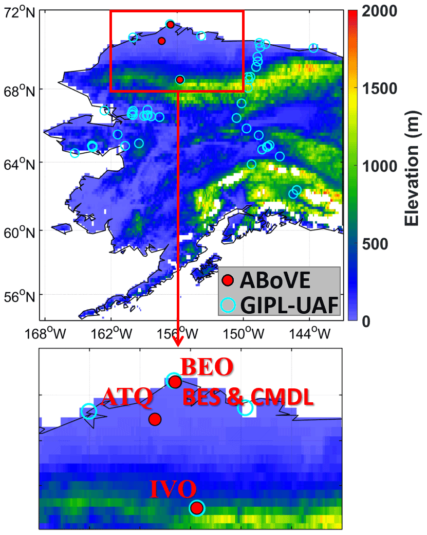
Figure 1Red dots indicate the five ABoVE flux tower sites used in this study. Cyan circles are GIPL-UAF permafrost sites.
ABoVE and CARVE provide soil temperature and moisture measurements at various depths from 5 to 40 cm. The Permafrost Laboratory, Geophysical Institute of University of Alaska Fairbanks (GIPL-UAF), provides daily subsurface soil temperature observations down to various depths at permafrost sites across Alaska (http://permafrost.gi.alaska.edu/sites_map, last access: 19 November 2021) (Romanovsky et al., 2009). We used the GIPL-UAF permafrost sites that are collocated with the ABoVE sites to complement the ABoVE observations at deeper depths, including BR2 (down to 15 m) and IV4 (down to 1 m). We first filled missing gaps vertically by fitting a polynomial to the soil temperature profile (Kurylyk and Hayashi, 2016) on a daily scale and then screened out outliers by examining the daily time series. Further, we aggregated both the ABoVE and the GIPL-UAF soil temperature measurements to ELMv1-ECA soil layer node depths using the inverse distance weighting method (Tao et al., 2017) and then averaged the two sets of aggregated observations. We used the assembled subsurface temperature observation datasets to evaluate the ELMv1-ECA simulated soil temperature profiles and the zero-curtain periods.
The observed soil moisture is only available at two or three depths that are quite different from model layer node depths and also show discontinuities in time. Thus, evaluation of ELMv1-ECA simulated liquid water content was limited. We matched soil moisture observations to the vertically closest model layer and then evaluated the simulated volumetric fraction of soil liquid water content at layers for time periods during which observations were available. In addition, we used ABoVE observed maximum soil moisture to infer site-scale soil porosity and then organic carbon content at IVO (see Sect. 3.2), which is used to prescribe thermal and hydraulic soil properties. Note that carbon substrate for respiration is simulated dynamically in the model (see Appendix B).
3.1 Modifications to E3SM land model (ELM)
The E3SM land model version 1 (ELMv1-ECA) couples essential biogeophysical and biogeochemical processes that solve terrestrial ecosystem energy, water, carbon, and nutrient dynamics (Golaz et al., 2019; Zhu et al., 2019). In the appendix, we describe in detail its subsurface soil thermodynamics, the carbon decomposition module, and the methane module that are of particular relevance to our study. Here we identify the potential problems of ELMv1-ECA that are responsible for the underestimation of cold-season CH4 and CO2 emissions and summarize the modifications made to ELMv1-ECA, emphasizing the model enhancements.
3.1.1 Phase-change scheme
We first improved ELMv1-ECA's numerical representation of coupled water and heat transport with freeze–thaw processes via improving the phase-change scheme. The freeze–thaw processes of soil water within ELMv1-ECA is simulated in a decoupled way; i.e., it solves soil temperatures ignoring the latent heat associated with phase change, determines the mass change of soil water required to adjust the initially solved soil temperature to the freezing point (i.e., 0 ∘C; Tf), adjusts the soil liquid and ice content by mass and energy conservation, and then readjusts temperatures after accounting for the heat deduction or compensation resulting from melting or freezing (see the detailed description in the Appendix A). The underlying assumption here is, taking the freezing process as an example, that the available liquid water at the initially solved temperature () will be completely frozen, releasing latent heat (Hi) to bring up back to Tf. Then, the estimated phase-change rate will be tuned down and the current temperature (i.e., Tf) will be readjusted if the to-be-increased ice mass is larger than the required mass change (−Hm) (see Eq. A4 in the Appendix A), which, however, only occasionally occurs. When the liquid water available to be frozen decreases enough, the released latent heat is not sufficient to compensate for the required energy deficit (), and then the freezing process stops. Consequently, the model freezes soil water quickly, resulting in an underestimated duration of the soil water phase-change processes and the zero-curtain periods, as well as cold-biased winter temperatures (Nicolsky et al., 2007; Yang et al., 2018a).
Here, we employed a phase-change efficiency and the temperature of the freezing-point depression to effectively solve the problem of overestimating phase-change rates within the current ELMv1-ECA modeling structure. These modification factors are explained below. The phase-change efficiency, introduced by Le Moigne et al. (2012) and adopted by Masson et al. (2013) and Yang et al. (2018a), introduces the dependency of available liquid water on the phase-change rate (Le Moigne et al., 2012). The phase-change efficiency for freezing, (see Eq. A9), is identical to the degree of moisture saturation or the volumetric fraction of soil liquid water content (i.e., , where is soil liquid water content and θsat, i is porosity). We applied the phase-change efficiency to the initially estimated energy and mass change involved, i.e., Hi and Hm (see Eq. A4 in the Appendix) when freezing or thawing processes occur.
As in Nicolsky et al. (2007) and Yang et al. (2018a), the occurrence of a phase-change process is then determined by the temperature of the freezing-point depression (i.e., an virtual temperature; see Eq. A10) instead of Tf. The virtual freezing-point depression temperature is reversely derived from the freezing-point temperature-depression equation (Fuchs et al., 1978; Cary and Mayland, 1972). With an upper limit as Tf, the virtual temperature describes the lowest temperature that can hold current liquid water content in the freezing soils. That is, the soil temperature has to be lower than the current virtual temperature to allow the freezing process to occur further.
We describe in detail the revised phase-change scheme in the Appendix A. In short, we improved the phase-change scheme of ELMv1-ECA by incorporating two modifications: (1) applying a phase-change efficiency to implicitly account for the heat compensation/deduction to the system from latent heat released/absorbed by soil water freezing/melting and (2) replacing the constant freezing point with the temperature of the freezing-point depression, as a virtual temperature, to determine the occurrence of phase change in subfreezing soils.
3.1.2 Environmental modifiers to the decomposition rate
We revisited ELMv1-ECA's representation for soil heterotrophic respiration dynamics in subfreezing soils and then scrutinized the environmental scalars of soil temperature and moisture. Within ELMv1-ECA's decomposition cascade model, the environmental factors that impact the decomposition rates of soil organic matter include soil temperature (fT), soil moisture (fW), oxygen stress (fO), and a depth scalar (fD) (See Appendix B). Within freezing and subfreezing soils, the soil water potential is related to temperature through the freezing-point depression equation (Niu and Yang, 2006). The current moisture factor fW, therefore, predicts zero respiration rates for subfreezing soils given a specific lower limit of soil water potential ψmin (−10 MPa; Eq. B2) (Oleson et al., 2013), as shown by Fig. S1a in the Supplement. We thus decreased the ψmin further to prevent zero respiration within the active layer when soil becomes subfreezing during cold-season months (Fig. S1b) as long as the soil water potential ψi exceeds the prescribed ψmin.
For wet soils, the factor that primarily limits the decomposition rates is oxygen availability (Sierra et al., 2017; Yan et al., 2018), since increases in soil moisture result in decreased dissolved oxygen. ELMv1-ECA approximates oxygen stress (fO) as a ratio of available oxygen to the demand by decomposers, which, however, is highly uncertain and unstable (Oleson et al., 2013). Some existing moisture scalars incorporate the oxygen stress together to account for the inhibition of decomposition in wet anoxic conditions, e.g., a moisture function proposed by Yan et al. (2018) and several functions tested in Sierra et al. (2015), including STANDCARB (Harmon and Domingo, 2001), Daycent (Kelly et al., 2000), Skopp (Skopp et al., 1990), and Moyano (Moyano et al., 2013). We thus also tested these existing moisture functions by replacing the original moisture scalar with them in the ELMv1-ECA. Particularly for the moisture function of Yan et al. (2018), we implemented it for each soil layer using the soil properties (i.e., porosity and clay content) of each layer and also tested it with different shape parameters and optimal wetness thresholds. When using the moisture scalars with built-in oxygen stress within ELMv1-ECA, the total environmental impacts on decomposition, , ftotal=fTfWfOfD, will be modified accordingly as ftotal=fTfWfD to avoid double counting of the oxygen stress.
ELMv1-ECA uses a Q10-based standard exponential function to account for the temperature effect on SOC decomposition (Eq. B1), with Q10 as 1.5 and Tref as 25 ∘C. Here, rather than striving for a single value of Q10 or a spatial map of Q10 as discussed in the introduction, or a particular individual temperature function, we seek a group of environmental modifiers (ftotal) that can correctly represent moisture and temperature sensitivity on heterotrophic respiration. Specifically, we assembled and tested 814 cases of ftotal using the newly modified moisture scalars and a variety of other empirical moisture and temperature functions, as documented by Sierra et al. (2015) and Yan et al. (2018). A full list of the specific moisture and temperature scalars tested is provided in Table S2.
3.1.3 Cold-season methane process
The ELMv1-ECA methane model solves the reaction and diffusion equation for CH4 and O2 fluxes with the Crank–Nicolson method. It includes the representations of CH4 production, oxidation, and three pathways of transport, including aerenchyma tissues, ebullition, and aqueous and gaseous diffusion (Riley et al., 2011). A short description of the ELMV1-ECA methane module is provided in Appendix C. The ELMv1-ECA methane model has been found to underestimate cold-season methane emissions over northern wetlands (Xu et al., 2016). The modifications to the phase-change scheme impact simulations of soil water and heat transfer (3.1.1); the changes in environmental scalar affect substrate availability (3.1.2). Both (3.1.1) and (3.1.2) influence soil heterotrophic respiration and could potentially lead to improvements in simulated CO2 and CH4 production but not necessarily CH4 emissions, which are also controlled by oxidation and transport mechanisms.
Here, we first modified the ELMV1-ECA CH4 transport mechanism in cold seasons by mimicking possible pathways for CH4 emissions from freezing and subfreezing soils. Specifically, we mimicked the emissions from ice cracks by plant aerenchyma transport (Zona et al., 2016), approximating the gas diffusion through ice cracks to the similar mechanism of diffusion through the aerenchyma tissues. Although in situ experiments demonstrated that, during winter, produced CH4 in frozen soils is predominately emitted to the atmosphere through vascular plants aerenchyma tissues (e.g., Kim et al., 2007), here we integrate the possible transport pathways including ice cracks and remnants of aerenchyma tissues together through Eq. (C3). Also, during the cold season over the tundra ecosystem, snow on the land surface provides strong resistance to CH4 transport to the atmosphere in ELMv1-ECA. But in reality, studies have shown methane can diffuse through snowpack at varying rates (Kim et al., 2007). We thus decreased snow resistance at the upper boundary by introducing a new scale factor when snow is present (Appendix C).
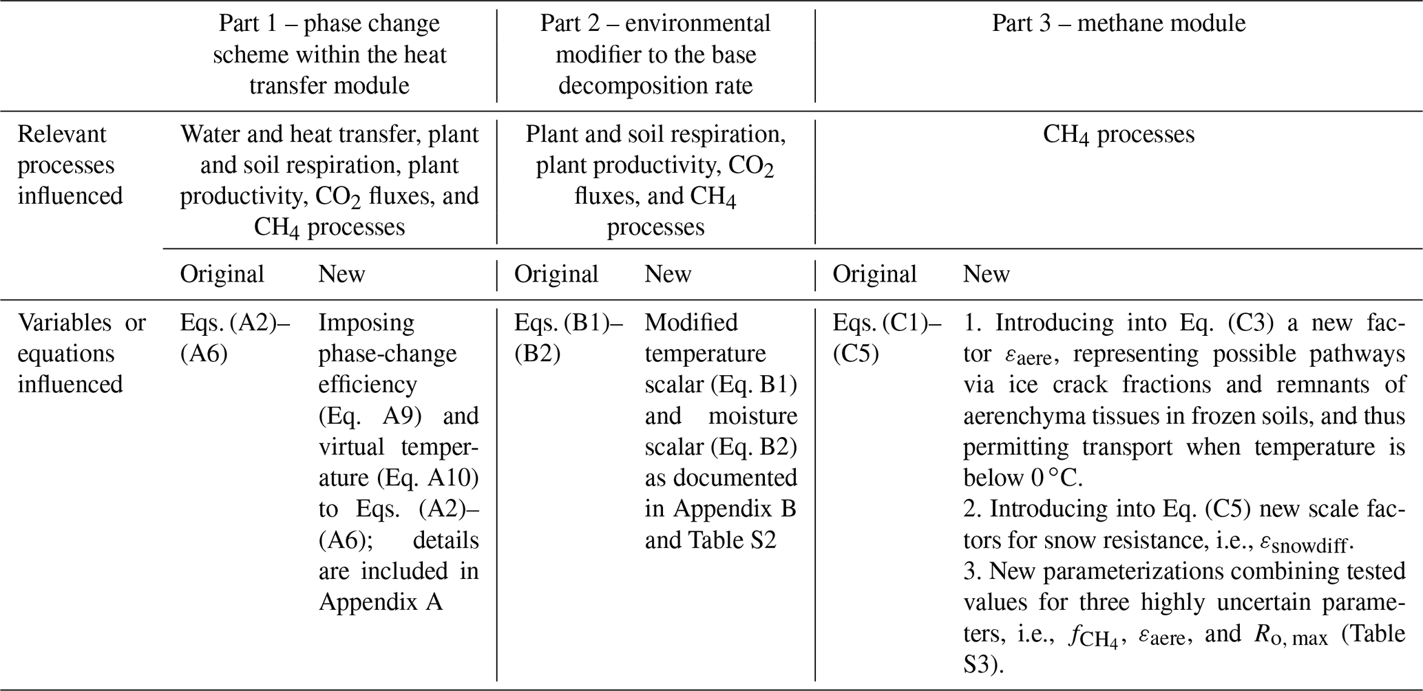
Table 1 summarized all the specific modifications made to ELMv1-ECA. These modifications involve new parameters that are all tuneable and can be systematically optimized via calibration. Here, we seek to reproduce the first-order cold-season process relevant to this study with the default formation and values listed in Table 1. We also conducted sensitivity tests on three variables three key parameters related to CH4 oxidation and transport processes and tested seven parameterizations (Table S3). The three CH4 process-related parameters include two key variables in the original CH4 model that have been reported to have a large uncertainty (Riley et al., 2011), i.e., (a fraction of anaerobically mineralized carbon atoms becoming CH4; Eq. C1) and Ro, max (the maximum oxidation rate constant; Eq. C4), as well as the newly introduced variable εaere (a factor representing remnants of aerenchyma tissues during cold seasons and possible pathways via ice cracks; Eq. C3). The sensitivity tests on CH4 process-related parameters were applied to the model with identified carbon decomposition schemes that predicted good simulations of CO2 flux (see Sect. 3.3).
3.2 Climate forcing, model configuration, and experiment design
We conducted transient simulations at 30 min temporal resolution driven by climate forcing from CRU JRA (Harris, 2019) from 1901 to 2017 at the four Alaska tundra site locations. Before the transient simulation, we conducted a 200-year accelerated decomposition (AD) spin-up period followed by a 200-year regular spin-up period (Koven et al., 2013b; Zhu et al., 2019) to initialize land carbon pools. Spin-up simulations start from a wet and cold condition. Specifically, subsurface temperatures were initialized as 274 K for the 1st to 5th soil layers, 273 K for the 6th to 10th layer, and 272 K for the 11th to the 15th layer, and volumetric soil water content was initialized fully saturated for all layers. In this manner, consistent vertical soil water content profiles were built in over the permafrost regions.
Baseline simulations were conducted with ELMv1-ECA default physics, parameters, and surface datasets, i.e., OriPC_OriDecomOriCH4 using original phase-change scheme, original decomposition scheme, and methane module (Table 2). To improve the model representation of the site-level soil environment, we first examined the global soil organic matter data at the ABoVE sites by evaluating ELMv1-ECA simulated subsurface soil temperature with the topsoil temperature prescribed to observations (as did in Tao et al., 2017). Using the top soil layer as the upper boundary, the modeling system excluded potential errors induced by inaccurate meteorological forcing and vegetation cover that impact the simulation of heat transfer from the atmosphere to the shallow soil (Tao et al., 2017). Then, the accuracy of simulated soil subsurface temperature is directly determined by the factors impacting heat transfer along the “shallow-to-deep soil” gradient (Koven et al., 2013a), e.g., soil thermal properties which are mostly determined by SOC content (Tao et al., 2017; Lawrence and Slater, 2008). Results well reproduced the subsurface soil temperatures except at IVO, where summer soil temperatures were notably overestimated (see Fig. S2a). This result indicates that the SOC content at IVO was too small, leading to a large thermal conductivity, small soil porosity, and small heat capacity, altogether resulting in fast penetration of heat into the subsurface soil during summer (Tao et al., 2017; Lawrence and Slater, 2008). Thus, we derived the organic matter density at IVO based on ABoVE soil moisture data through a linear relationship between SOC content and soil porosity (i.e., Eq. 3 in Lawrence and Slater, 2008), assuming the observed maximum volumetric water content was porosity (see Fig. S3 for details). With the newly derived profile of soil organic matter density at IVO, the simulation showed large improvements in summer soil temperatures compared to that using the original global carbon dataset (see Fig. S2b). The derived SOC content is also consistent with the organic layer thickness reported in Davidson and Zona (2018). Hereafter, the simulations at IVO presented in this paper use the newly derived organic carbon data without repeated clarification.
Table 2List of designed experiments.

a “NewCH4” uses the newly modified methane module with default
parameterization (see Table S3 in the Supplement).
b “NewDecom” means replacing the original temperature- and
moisture-dependency functions on decomposition rates with (814) new
functions of environmental modifiers as listed in Table S2 in the Supplement. “NewCH4” here means the newly modified methane module
with seven parameterizations (Table S3). The seven CH4 parameterizations
were iteratively applied to the model together with 160 common carbon
decomposition schemes that provide good performance for CO2 flux (i.e.,
NSE_CO2 >0.5) at all the sites. This
resulted in 1934 “NewPC_NewDecomNewCH4” simulations in
total (i.e., ).
c “NewPC_Optimized” is the optimal simulation among the
1934 NewPC_NewDecomNewCH4 cases at each site.
d “NewPC_Generic” means the simulation with the
identified generic parameterization that can be applied to regional
simulation. The generic scheme is the common satisfactory scheme that
provides the best overall performance for all the sites.
The representative spatial scale of the eddy flux tower is small compared to the grid cell of global surface datasets and the climate forcing data used by ELMv1-ECA, although the forcing dataset was interpolated to the site scale with a bilinear or nearest-neighbor method. The site-scale vegetation cover also shows a large diversity of vegetation types according to the detailed vegetation survey at ABoVE flux tower footprints obtained in 2014 (Davidson and Zona, 2018). The ELMv1-ECA's default plant type function (PFT) dataset was derived from satellite-based data by Lawrence et al. (2007). We analyzed the vegetation composition from the closet survey plot to the flux tower and examined the rationality of ELMv1-ECA's percentage of PFT for the site-scale simulation through testing different PFT datasets derived from this vegetation survey (Davidson and Zona, 2018). We found that these PFT datasets generally are not superior to the original PFT dataset, which generally reproduced satellite-based gross primary production (GPP; Fig. S4). We thus confirmed that ELMv1-ECA's PFT dataset was a good compromise between representing the site-scale ecosystem and other global parameters and surface datasets within the model. The surface CH4 emission is a weighted average of simulated saturated and unsaturated components using predicted inundation and non-inundation fractions. To compare simulated CH4 emissions with ABoVE measurements at the site scale, we use the estimated inundation fractions at the footprint of ABoVE eddy-covariance flux towers (see details in Xu et al., 2016).
Table 2 lists the experiments conducted in this study. We modified each model component (i.e., the heat transfer model, carbon decomposition model, and methane model) serially. All the experiments ran through 1901 to 2017 with spin-up as described earlier, although the evaluation and optimization were conducted only using results from 2013 to 2017. We first ran simulations with the 814 environmental modifiers together with the modified methane model with default parameterization (Table S3). Then, we selected the environmental modifiers that provided satisfactory performance in simulating CO2 flux, and we repeated simulations with the seven CH4 parameterizations (Table S3). Among all the simulations results, we identified an optimal simulation for each site (see details in Sect. 3.3).
3.3 Evaluation metrics, optimization method, and trend analysis
We define the early cold season as September and October; the cold-season period as September to May, which includes the two shoulder seasons (both thawing and freezing) as consistent with Zona et al. (2016); and the warm season from June to August. We define the zero-curtain period (ZCP) as the set of successive days when the soil temperature is within the range of [−0.75, 0.75 ∘C] starting in fall (i.e., the freezing season) based on Zona et al. (2016). We computed the ZCP duration for each soil layer every year from 1950 to 2017 and estimated the historical trend as the regression slope between ZCP duration and time. Similarly, we estimated the trends of cold-season CH4 and CO2 emissions through linear regression analysis. A p value of 0.05 is used to determine if the computed trend is statistically significant. Results for ZCP duration and trend vary with soil depths; thus, we choose a common modeling depth at which the ZCPs show significant trends for all the sites, to give an example.
To evaluate ELMv1-ECA simulated soil temperature and moisture, we calculated the RMSE for each soil layer, i.e., , where and Ot are simulated and observed soil temperature or moisture, respectively, and t is a daily time step. We used the mean absolute error (MAE), i.e., to assess the simulated duration of ZCP of each soil layer. Note that, depending on the amount of soil liquid water content, the whole course of the freezing process may or may not entirely fall into the ZCP; i.e., the ending time of ZCP does not necessarily align with the end of the freezing process. The onset of freezing, though, is always later than the starting day of the ZCP, and the main course of the freezing process is still within the ZCP.
Here the modeled active layer thickness (ALT), i.e., maximum thaw depth during an annual cycle, is computed as the bottom depth of the deepest thawed soil layer (i.e., with a maximum annual temperature above 0 ∘C) further extended down to the possible non-frozen fraction of the layer below, as in Tao et al. (2019, 2017). We only derived the length of ZCP for soil layers with a maximum annual temperature above 0 ∘C since limited phase-change processes occur in deeper layers. Then, the soil layers containing or below the permafrost table have a zero-day ZCP. We computed the MAE of ALT simulated with both the original (OriPC) and the new phase-change (NewPC) scheme. Also, we computed the relative improvement in simulated soil temperature (Ts) and ZCP compared to the baseline results. Specifically, we calculated 100 % × (RMSE_Ts_OriPC − RMSE_Ts_NewPC) RMSE_Ts_OriPC and 100 % × (MAE_ZCP_OriPC − MAE_ZCP_NewPC) MAE_ZCP_OriPC to quantify the enhancement by employing the new phase-change scheme.
We used Nash–Sutcliffe efficiency (NSE) (Nash and Sutcliffe, 1970) to examine the performance of the ELMv1-ECA simulated time series of CH4 and net CO2 fluxes in comparison with assembled observations (Sect. 2) at the monthly timescale. The NSE ranges from negative infinity to one, calculated as Eq. (1):
where t means monthly time step, N is the total number of time steps, and Ot are simulated and observed flux at time step t, respectively, and σo is the standard deviation of observations. Note we only used observed monthly averages when the number of daily observations was more than 20 d. The model performance is generally considered satisfactory with an NSE >0.50 (Moriasi et al., 2007) and perfect with an NSE as one. To simultaneously evaluate CH4 and CO2 fluxes, we combined both and in the form of , representing the distance from (, ) to (1, 1) in a coordinate plane with x axis as and y axis as . Then, the optimal simulation thereby is the one having the shortest distance to the ideal scenario (1, 1). We also define a satisfactory model performance in terms of simulating CH4 and CO2 fluxes as the case with both and larger than 0.5.
We optimized the model simulations through two steps. Specifically, we first evaluated the simulations using (814) environmental modifiers to the base decomposition rate that assembled commonly used empirical soil temperature- and moisture-dependency functions (Table S2). These simulations used the newly modified methane model with the default parameters (Table S3). We selected the common decomposition schemes that provided satisfactory results of CO2 flux for all the sites (i.e., >0.5). Then, we iteratively repeated simulations with the common carbon decomposition schemes along with the seven CH4 parameterizations (Table S3). Among all these simulations (NewPC_NewDecomNewCH4; Table 2), we identified an optimal simulation for each site that has the smallest distance from (, to (1, 1) (i.e., dist); the environmental modifier to the base decomposition rate and the methane parameterization used in the optimal simulation is the optimized parameterization for this site.
Further, among the common parameterizations of environmental modifiers and CH4 parameterizations that show satisfactory performance both in CH4 and CO2 fluxes for all the sites, we identified a generic scheme as the one providing the minimum Euclidean distance in a site-performance space, calculated as , where n is number of sites. The generic scheme then is the common satisfactory scheme that provides the best overall performance for all the sites and can be applied for the regional simulation over Alaskan North Slope tundra.
In general, we use NSE to evaluate the model's performance in capturing seasonality (i.e., time series) of CH4 and net CO2 fluxes and optimize CH4 and CO2 simulations. We use RMSE and MAE to assess the model's capability in simulating the magnitudes of soil temperature, moisture saturation, ZCP durations, and cumulative CH4 and CO2 emissions.
4.1 Evaluation of soil temperature and zero-curtain period
We first evaluated the simulated daily soil temperature profiles against the observations from ABoVE and GIPL-UAF at the four site locations. Then, we examined improvements in simulations of soil temperature, soil moisture, and the durations of ZCPs by employing the newly revised phase-change scheme (i.e., NewPC_OriDecomOriCH4; Table 2).
Results for the BES/CMDL and IVO site are shown in Fig. 3; results for other sites are shown in Fig. S4 in the Supplement. At BES/CMDL, the baseline (i.e., OriPC_OriDecomOriCH4; Table 2) simulated soil temperatures (Ts) with the default phase-change scheme (Ts_OriPC; blue lines; Fig. 2a) decrease rapidly in fall due to the overestimated freezing rate (i.e., the slope of decreasing liquid water fraction), notably underestimating the duration of the ZCP (bluish shaded area). Consequently, liquid water saturation (Sf_OriPC, green lines; Fig. 2a) quickly drops to a lower bound (i.e., the supercooled liquid water content divided by porosity), and the freezing process generally completes within a short period (days for top layers to 1 month at the most for deeper layers). The baseline model soil temperature drops (Ts_OriPC) sharply after the freezing process ends (i.e., Sf_OriPC decreases to the lower bound). In contrast, the new phase-change scheme effectively slows freezing rates, showing relatively smaller slopes of decreasing liquid water saturation (Sf_NewPC; magenta lines; Fig. 2a) within the ZCPs than the baseline simulation (Sf_OriPC; green lines) especially in the fourth and fifth layer. Hence, the gradually released latent heat maintains soil temperatures around the freezing point for a longer period (Ts_NewPC; red lines; Fig. 2a), effectively extending the ZCPs (reddish shaded area), which agree better with observations (gray shaded area) than the baseline results. The ZCP duration increases with depth and can extend into December for deep soil layers. Similarly, improved performance was found at the BEO and ATQ sites (Fig. S4 in the Supplement). At IVO, however, while the new phase-change scheme greatly improved simulated results relative to the baseline simulation (Fig. 2b), the model still slightly underestimated ZCP durations and also underestimated winter (December to April) soil temperature (red vs. black). This result at IVO is consistent with the underestimation of late-season soil liquid water available to be frozen and thereby to release sufficient latent heat (Fig. S5). In general, the improvements in ZCP are larger in deeper layers than topsoils, with the top layer showing only marginal improvement.
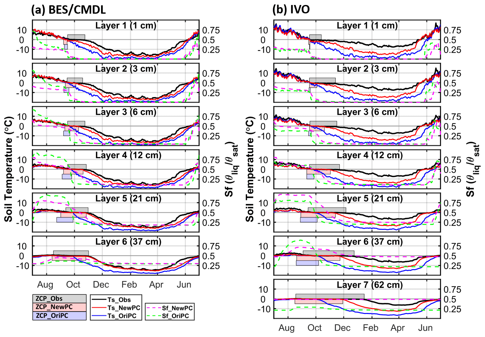
Figure 2Comparison of multi-year (2013–2017) averaged daily soil temperatures observed (Ts_Obs, black) and simulated with the original (Ts_OriPC, blue) and improved (Ts_NewPC, red) phase-change schemes at BES/CMDL (a) and IVO (b). Simulated moisture saturation with the original (Sf_OriPC; green) and improved (Sf_NewPC; magenta) schemes is shown on the right y axes. Here, the moisture saturation means soil unfrozen (liquid) water content. The horizontal axes indicate days from July to June, with ticks representing the first day of each month. Shaded areas represent durations of zero-curtain periods observed (ZCP_Obs, gray) and simulated (ZCP_OriPC, blue; ZCP_NewPC, red). No baseline ZCP is shown in the sixth layer for BES/CMDL and the seventh layer for IVO because the maximum annual temperature is below 0 ∘C.
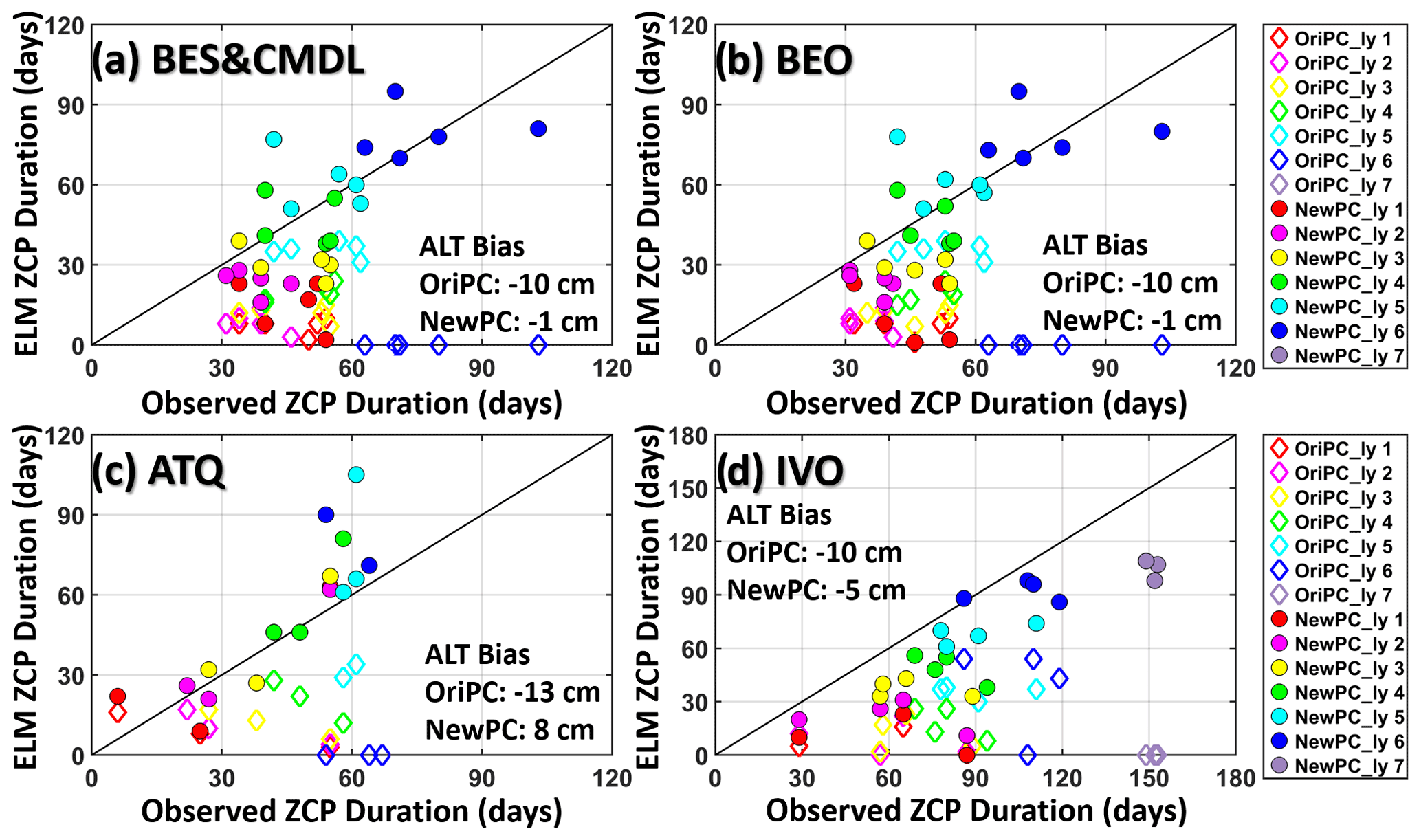
Figure 3Comparison between observed and ELMv1-ECA simulated durations of ZCP for the original (OriPC; open diamonds) and improved (NewPC; solid circles) phase-change schemes over four annual cycles (July to June) from 2013 to 2017. “ly” means model layer. Simulated ZCP durations with NewPC demonstrate significant improvements compared to OriPC (solid dots vs. open diamonds), especially for the fourth to the deepest layer above permafrost. Note that a zero-day ZCP means that the maximum daily temperature during an annual cycle is below 0 ∘C. The pairs of zero vs. non-zero-day ZCP (e.g., OriPC_ly 7 at IVO and OriPC_ly 6 at other sites) indicate that baseline results underestimated ALT. The bias (simulation − observation) of multi-year averaged ALT simulated by the two experiments is provided in each panel.
Simulated ZCP durations with the revised phase-change scheme (NewPC) demonstrated notable improvements over the baseline (original) phase-change scheme (OriPC) (solid circles vs. open diamonds) (Fig. 3), showing greatly reduced mean absolute errors (MAEs) (Table 3). For example, at 12 cm depth (fourth layer), the relative improvements in MAE of the ZCP durations were 65 %, 65 %, 66 %, and 50 % for the four site locations (Table 3). The largest improvement in MAE was as large as 65 d for the sixth layer at BES/CMDL, with a relative improvement of 84 % (Table 3). This large improvement stems from the better-estimated ALT at this site; the OriPC simulated sixth-layer temperature remained below freezing, leading to a zero-day ZCP (diamonds on the x axis in Fig. 3). The new phase-change scheme not only improved simulation of the ZCP and cold-season soil temperatures, but also affected the warm-season dynamics and thus ALT estimates. As Fig. 3 indicates, the NewPC improved simulated ALTs at all four site locations with reduced bias in multi-year averaged ALT, resulting in more reasonable ZCP durations for the sixth layer (and also the seventh layer for IVO), while the baseline results were zero days.
Table 3Mean absolute error (MAE) of simulated ZCP (days) with the original phase-change scheme (Ori_PC) and newly resized phase-change scheme (NewPC), and the relative improvement (%) of using the new phase-change scheme compared to the baseline results, calculated as 100 % × (MAE_ZCP_OriPC − MAE_ZCP_NewPC) MAE_ZCP_OriPC.
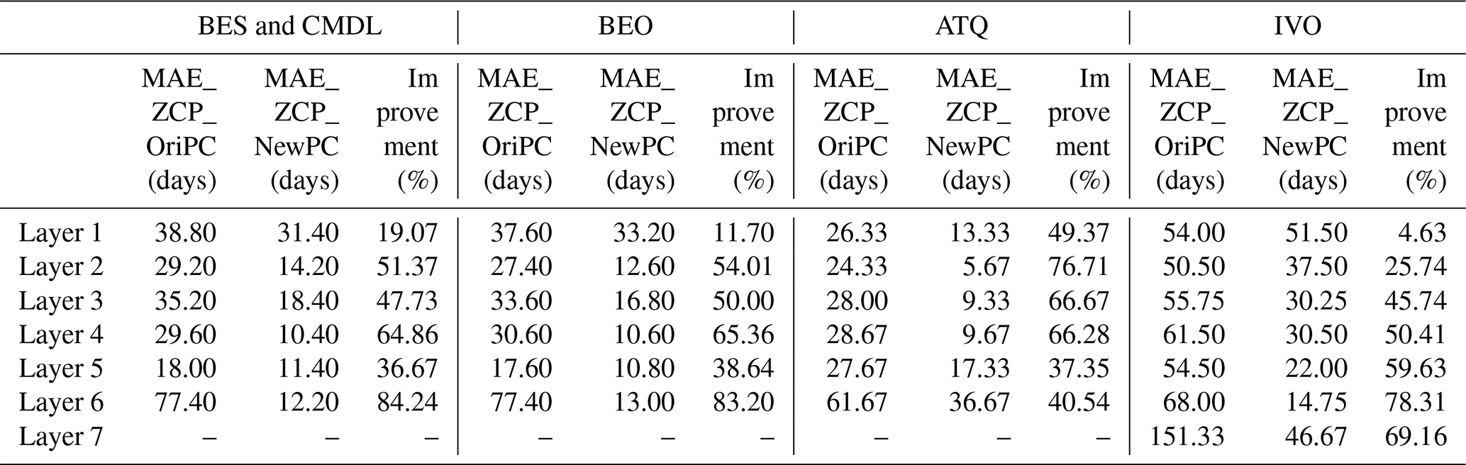
The deeper active layer simulated by NewPC implies more soil water storage capacity, resulting in lower soil moisture in shallow soil layers and higher soil water in deep layers (Sf_NewPC; magenta lines; Fig. 2) compared to baseline results. The changes in soil liquid water content, in turn, impact phase-change and soil temperature simulations. Comparison with the observed soil liquid water content reveals a better agreement with observations (Table S5). For example, at ATQ (Fig. S7), the RMSEs of the liquid water content were reduced by 5.4 %, 35.3 %, 42.6 %, and 25.4 % for the third through sixth layers, respectively (Table S5).
The changes to model representations of phase change led to large reductions in soil temperature bias. The relative improvements in RMSE of simulated soil temperatures during September and October (i.e., the 2 months that the ZCPs usually cover) generally increased with depth for surface layers (within about 20 cm of the surface, i.e., first to fourth layer) and were above 80 % for the intermediate layers (fifth to eight) at all the sites (Fig. 4). At the two Barrow sites where observed soil temperatures were available, the relative improvements for the deepest (13th) layer were 72.6 % and 71.1 %, on average, for the early winter and annual cycle, respectively. Therefore, incorporating the new phase-change scheme also resulted in improved bottom temperature boundary conditions, which is critical for accurately simulating permafrost dynamics (Sapriza-Azuri et al., 2018). Improvements between September and December and the whole annual cycle also increased with soil depth, showing site-averaged reductions in RMSEs ranging from 47 % to 63 % and from 36 % to 46 % for the two periods, respectively. The whole cold-season period (September to May) showed, on average, 44 % to 53 % reduction in RMSEs from the first to sixth layer at relatively warmer sites (i.e., ATQ and IVO) and a reduction from 19 % to 69 % for the top 13 layers for the two Barrow sites. Also, after the freezing process ends, simulated deeper soil layer temperatures were underestimated (e.g., December through April). This bias might be caused by underestimated snow depth (Fig. S9) possibly resulting from inaccurate forcing (particularly snowfall), land cover, microtopography, and/or windblown snow redistribution.
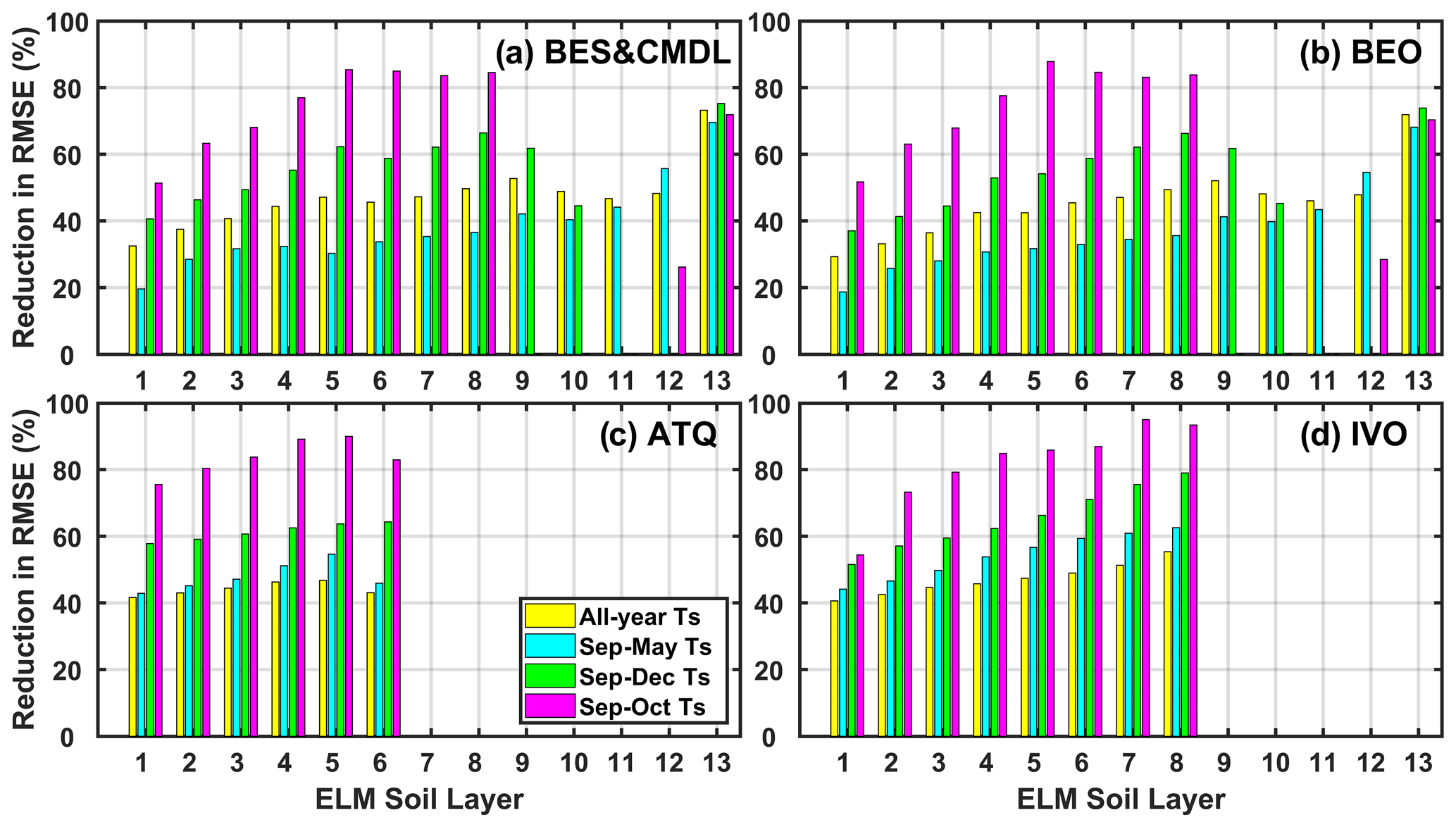
Figure 4Relative improvement in the RMSE of simulated soil temperature with the new phase-change scheme (RMSE_Ts_NewPC) compared to that with the original scheme (RMSE_Ts_OriPC), calculated as 100 % × (RMSE_Ts_OriPC − RMSE_Ts_NewPC) RMSE_Ts_OriPC.
Simulations with the new phase-change scheme also show improved agreements between simulated and observed soil temperatures during the spring thawing season compared to the baseline results (red vs. blue in Fig. 2). Compared to observations, the newly simulated soil temperatures were still slightly underestimated during the thawing season (i.e., May) at all four sites, showing later onset of thawing indicated by the timing when warming soil temperatures cross 0 ∘C and soil moisture starts to rise (Fig. 2). One possible reason for this bias is the lack of representation of advective heat transport. That is, the model does not represent the heat of spring rain that is advectively transported into soils (Neumann et al., 2019; Mekonnen et al., 2020), nor does it account for advective heat transport associated with water fluxes in subsurface soils after the spring–rainwater mix with existing cold liquid water in soils.
The improved simulations of soil temperature, liquid water content, and ZCP duration greatly impacted soil HR and methane production but did not necessarily guarantee improvements in CO2 and CH4 emissions. In the next section, we closely evaluate simulated CH4 and CO2 fluxes with different parameterizations of environmental modifiers and the modified CH4 parameterizations as described in Sect. 3.1.
4.2 Evaluation of CO2 and CH4 fluxes
Here we evaluate the simulated monthly CO2 and CH4 fluxes at the site scale against EC tower observations. Figure 6 displays the NSEs of ELMv1-ECA simulations using different carbon decomposition schemes and CH4 process-related parameters, i.e., NewPC_NewDecomNewCH4 (gray dots) (see configurations in Table 2). (Time series of all the simulations are provided in Fig. S7.) The failure of simulated CH4 emissions to capture the methane seasonality at IVO (as indicated by Figs. S8 and S10) might occur because of the lack of (1) a reasonable wetland module that can adequately account for inundated hydro-ecological dynamics, (2) advective heat transport at the air–ground interface through rainfall infiltration and within subsurface soils through water transfer, (3) a representation of microbial dynamics, and (4) the geological micro-seepage emission of CH4, as reported in previous studies (Anthony et al., 2012; Etiope and Klusman, 2010; Russell et al., 2020). For instance, Lyman et al. (2020) showed large temporal variability of CH4 at natural gas well pad soils, similar to the observations at IVO (Anthony et al., 2012). The advective heat transport not only impacts soil temperature, but also affects soil moisture redistribution, substrate availability, and microbial activity. Also, methanogen seasonal dynamics would cause hysteretic effects on CH4 emission response to soil temperatures (Chang et al., 2020; 2021; Chadburn et al., 2020). In the future, we will incorporate a representation of methanogen seasonal dynamics and simulate microbial population and activity levels to address the hysteresis of CH4 emissions with temperature. We will also explore more on the contribution of geological micro-seepage emission. The four mechanisms discussed above (i.e., wetland dynamics, advective heat transport, microbial dynamics, and geological micro-seepage CH4 emission) currently missing in our model are likely necessary to simulate CH4 emissions at this site, and we therefore do not include CH4 analysis at IVO in the following sections.
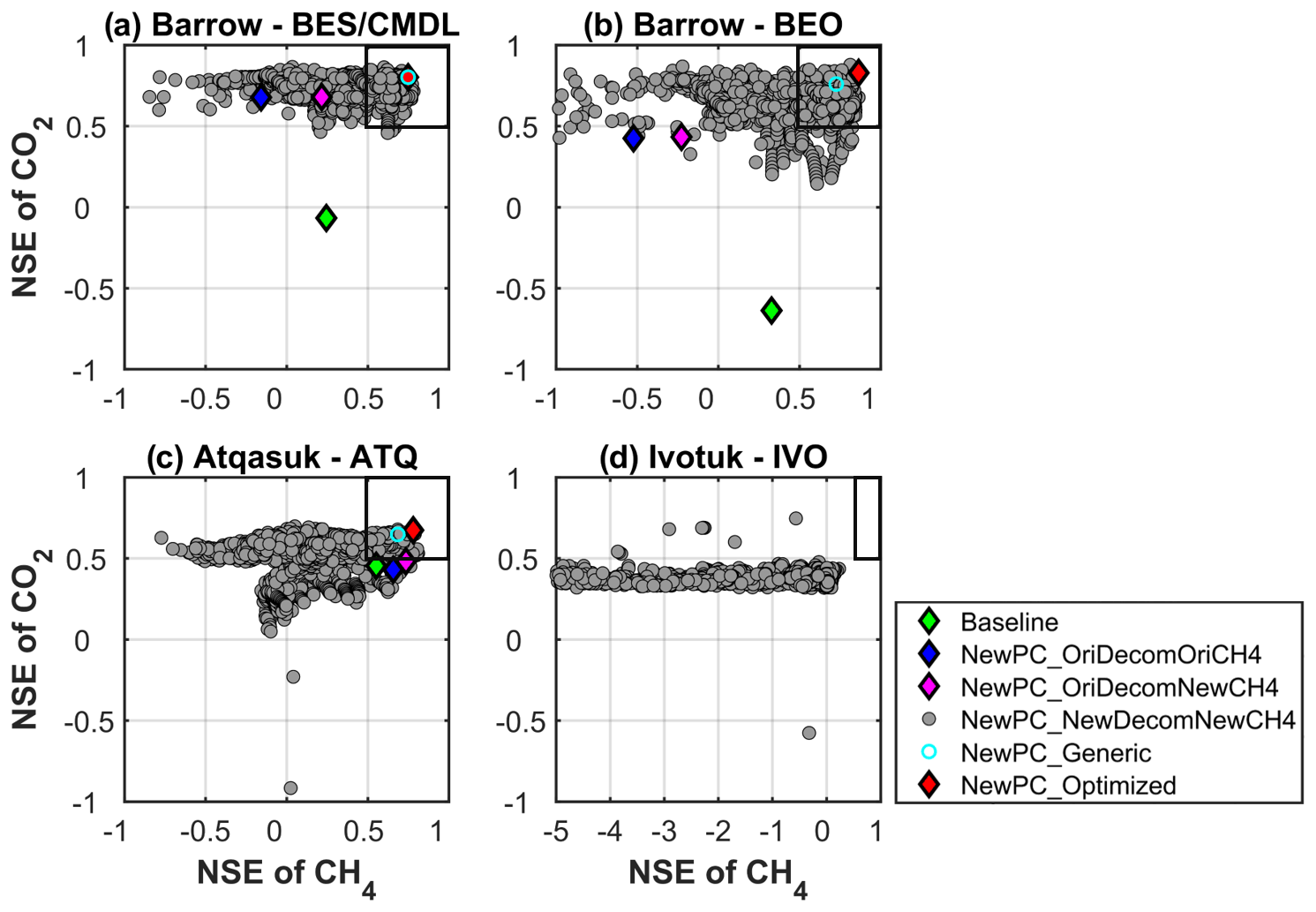
Figure 5Scatter plot between the Nash–Sutcliffe efficiency (NSE) of simulated monthly CH4 and CO2 emissions. An ideal simulation has both NSEs of CH4 and CO2 as one (i.e., the upper right corner). The boxes encompass simulations with satisfactory performance (NSE >0.5). Optimized (red) – the best simulation for each site; generic (cyan) – the simulation with a common parameterization of carbon decomposition scheme and CH4 parameter scheme that provides best overall performance for all the sites. See Table 2 for the configuration for each experiment. The gray dots represent all the tested (1934) simulations indicated in the annotation of Table 2. Symbols outside the plotting ranges indicate poor performance, e.g., (−34.9, −0.3) for baseline at IVO, and thus are not shown in the figure.

Figure 6Observed and simulated monthly CO2 (a.1, b.1, c.1, d) and net CH4 (a.2, b.2, c.2) flux with the baseline model (ELM_Baseline) and the experiments with updated models (see Table 2 for the configuration for each experiment). Shaded gray areas indicate the minimum-to-maximum bound of simulations within the good performance zone (as shown in Fig. 5). Black open circles are observed monthly averages with the number of daily observations less than 10 d, which are not used for the computation in Fig. 5. “ELM_NewPC_Optimized” means the best simulation for each site (red diamonds in Fig. 5). Intermediate results including “ELM_NewPC_OriDecomNewCH4” is included in Fig. S8 in the Supplement.
The improved phase-change scheme, and thus improved simulations of ZCP durations and soil temperature and moisture, resulted in greatly improved performance for CO2 emissions at BES/CMDL and BEO and in slightly better performance for CH4 emissions at ATQ, compared to the baseline (blue for NewPC_OriDecomOriCH4 vs. green for baseline; Fig. 5), even though the carbon decomposition and methane model remained the same as the baseline. Incorporating the revised CH4 model with the default parameter (discussed in Sect. 3.1.3) improved simulated CH4 emissions at BES/CMDL, BEO, and ATQ (magenta for NewPC_OriDecomNewCH4 vs. blue for NewPC_OriDecomOriCH4), especially during the cold season (Fig. S8). The improved NSEs for CH4 emissions mainly resulted from increased emissions over early winter (September and October) and slight but persistent enhancements throughout the rest of the cold season (magenta in Fig. S8), which were related to our modifications to CH4 transport mechanisms. Further, with the identified optimal parameterization of environmental modifiers to the base decomposition rate and methane parameters, results demonstrate substantial improvements to the simulation of net CO2 flux and CH4 emissions compared to baseline results (red vs. others; i.e., shortest distance from (, to (1, 1)). Among the 121 common schemes providing good performance for both CO2 and CH4 emissions (i.e., both and larger than 0.5, indicated by the gray dots within the boxes in Fig. 5), we identified a generic scheme by selecting the common parameterization that provided the best overall performance for all the sites (except IVO) (cyan; Fig. 5). The specific environmental modifier functions and methane parameters for the optimal and generic scheme are provided in Table S6.
Figure S8 illustrates the uncertainty associated with the model representations of environmental influences on heterotrophic respiration and methane parameters. The optimal simulations at the study sites used either the modified ELMv1-ECA moisture scalar or Yanetal (see Table S6), i.e., two groups of moisture-dependency functions implemented for each soil layer. For the Sierra et al. (2015) empirical moisture functions, the influence of liquid moisture content on heterotrophic respiration is uniformly applied to all active soil layers, even though the soil properties (e.g., porosity and saturated soil water potential) are quite different vertically. ELMv1-ECA's moisture scalars (including the original scheme) that use soil water potential, in contrast, reasonably explained the varying influence along with the vertical soil profile (i.e., relationships between soil liquid water content and soil temperature varies with soil clay fraction as demonstrated by Fig. 1 in Niu and Yang, 2006). The Yanetal moisture functions also used soil-layer-dependent porosity and clay content to calculate relevant parameters (Yan et al., 2018). The simulations with moisture functions documented in Sierra et al. (2015) generally overestimated CO2 and CH4 emissions, especially during the warm season when the thaw depth is deep and soil wetness is high, thus permitting large moisture modifier scalar to be applied to the base decomposition rates for all the soil layers regardless of soil properties.
Reducing the minimum soil water potential ψmin for moisture scalar effectively prevents the possibility of zero respiration in subfreezing soils during wintertime (Fig. 6). This change exerts more impact on cold sites, such as the two Barrow sites, due to the smaller supercooled liquid water under the colder temperature. Thus, the improved NSEs for CO2 and CH4 emissions at BES/CMDL and BEO were larger than those at ATQ (Fig. 5). Since the temperature at ATQ was not cold enough to make the supercooled liquid water content small enough to give a zero moisture scalar, the microbial respiration was not completely shut down with the original decomposition modifier at this site. Indeed, at ATQ, where cold-season temperatures are relatively warmer than at BES/CMDL and BEO, simulations with the original ELMv1-ECA environmental modifier (i.e., NewPC_OriDecomNewCH4 in Fig. S8; discussed in Sect. 3.1.2) already released much more CO2 and CH4 throughout the cold season than in the baseline simulations, owning to the improved simulations of soil temperature and moisture, as well as the modifications for CH4 transport. At IVO, although generally showing low NSEs for CH4, some new simulations have greatly improved values that are larger than 0.5 (Fig. 5), compared with −0.3 for baseline. Indeed, the best result at IVO (with a 0.78) significantly improved the simulation of summer CO2 sink compared to baseline result (Fig. 6).
The optimal simulations used Daycent2 temperature-dependency function at ATQ and Q10-based temperature functions at BES/CMDL and BEO with high Q10 values (e.g., 2.0 and 2.5, respectively) (Table S6), mutually mediating the response of microbial respiration with moisture functions discussed above. At all three sites, the optimized parameterizations used a higher εaere (i.e., 0.05; Table S6), representing possible cold-season CH4 emissions through ice cracks and remnants of aerenchyma tissues. This newly introduced variable is highly uncertain, although it can be calibrated at any other site against cold-season measurements. At BES/CMDL, the optimized parameterization used a decreased maximum CH4 oxidation rate constant which has been reported to be highly uncertain, especially over high latitudes (Riley et al., 2011). The generic scheme (i.e., carbon decomposition + CH4 parameters) overlaps with the optimized parameterization at BES/CMDL, which provided the best overall performance at all three sites (Table S6). Despite the small site number and the limited spatial representativeness of each site, the identified generic scheme might be applied to the Alaska North Slope tundra. Nevertheless, the generic scheme might induce uncertainty in simulations and might not be the optimal regional scheme over other ecosystems or given different climate forcing and soil conditions. Still, we conclude that the generic scheme can serve as a reasonable initial scheme for estimating CO2 and CH4 emissions over other high-latitude areas (e.g., Fig. S11). In the future, we will explore more sites from newly published CO2 and CH4 datasets from pan-Arctic ecosystems, e.g., BAWLD-CH4 (Kuhn et al., 2021) and FLUXNET-CH4 (Delwiche et al., 2021; Knox et al., 2019).
The extended ZCPs, the revised environmental modifier to decomposition, and the modified CH4 transport mechanism and oxidation parameter together resulted in large improvements for both CO2 and CH4 emissions, especially over the cold season. Nevertheless, the optimal simulations still overestimated the contribution of the early-cold-season (September and October) CO2 emissions at BEO and ATQ (top panel; Fig. 7) and underestimated CH4 emissions during post-ZCP months (e.g., October to December) (bottom panel; Fig. 7). There are many reasons for the early-cold-season CO2 overestimations, including model deficiencies, prescribed land parameters, and possibly inaccurate forcing. As for the underestimations of post-ZCP carbon emissions, one critical reason is the lack of sudden bursts of CO2 and CH4 within the model, i.e., the gases are pushed out of freezing soils during the freeze-up period (Mastepanov et al., 2008; Pirk et al., 2017). Currently, the ELMv1-ECA mimics this sudden burst mechanism by preventing CO2 and CH4 from dissolving in the soil ice fraction (Riley et al., 2011), which could capture some burst emissions (e.g., CH4 emissions in October and September of 2013 at ATQ; Fig. 6); but it still shows an overall underestimation for sudden-burst emissions, especially at colder sites (e.g., BES/CMDL and BEO; Figs. 6 and 7). We will improve this mechanism in the future by explicitly simulating ice-encroaching soil pores and pushing out gases and liquid water out of the soil matrix. In the next section, we quantify the cold-season contribution of CO2 and CH4 emissions and then estimate the historical trends of seasonal CO2 and CH4 emissions from 1950 to 2017.
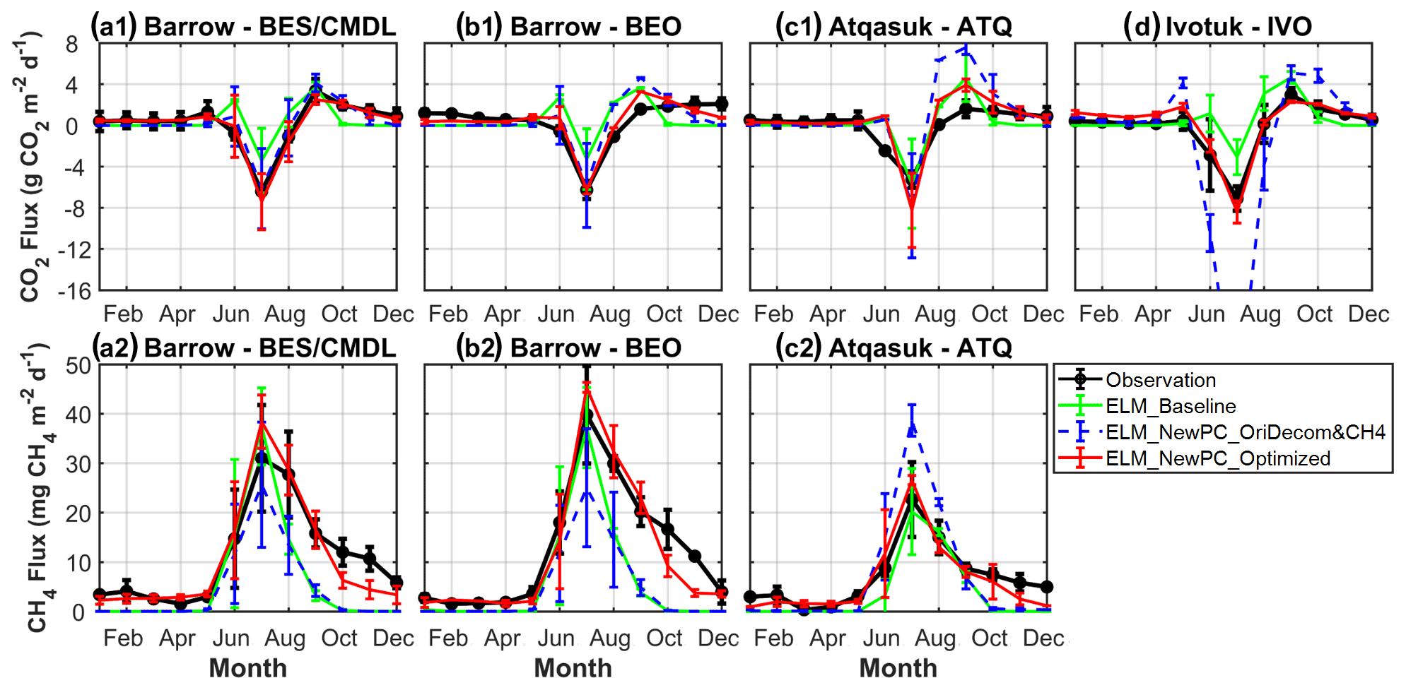
Figure 7Comparison of multi-year (2013–2017) averaged monthly mean net CO2 flux (a1, b1, c1, d) and CH4 emissions (a2, b2, c2) from simulations and measurements at the study sites. The error bars represent standard deviation of monthly mean.
4.3 Cold-season contribution of CH4 and CO2 emissions and historical trends
Throughout this section, we only retain and discuss the identified optimal simulation results (i.e., ELM_NewPC_Optimized) for each site. To better verify the cold-season contribution of CH4 and CO2 emissions to the annual budget, a multi-year average approach was taken because of discontinuity in the observed time series.
The new simulation results with the optimal parameterization showed greatly enhanced performance in terms of capturing the averaged seasonal cycle (red; Fig. 8), especially for the cold-season months (September to May; Fig. 8), reducing site-averaged MAEs in cold-season total CH4 and CO2 emissions by 72 % and 70 % (Fig. 8, Table 4), respectively. Specifically, compared to baseline results which significantly underestimated the cold-season carbon emissions, the optimized simulation results showed 0.79 and 44.0 gC m−2 increases in site-averaged cold-season CH4 and CO2 emissions, respectively. The optimized simulations reduced biases in early-cold-season (cold-season) CH4 emissions by 80 % (74 %), 86 % (76 %), and 77 % (61 %) for BES/CMDL, BEO, and ATQ (Table 4), respectively. The observed cold-season CH4 emissions contributed at least ∼40 % to the annual total at three of the study sites, of which about half occurred in early-cold-season months (September and October) (Fig. 8; Table 4), i.e., the 2 months hosting the major part of ZCPs for the top to intermediate soil layers. The simulated contributions of early-cold-season (September and October) CH4 emissions to the cold-season total were 51 %, 65 %, and 55 % for the three sites, in comparison with the observed 47 %, 58 %, and 43 %, showing slight overestimations. Compared to the baseline-simulated percentage of cold-season contributions to the annual total CH4 emissions (i.e., only 5 %, 6 %, and 15 %), the optimized simulation showed greatly improved agreements with observed contributions, i.e., 35 %, 35 %, 33 % vs. 45 %, 42 %, 45 % for BES/CMDL, BEO, and ATQ, respectively.
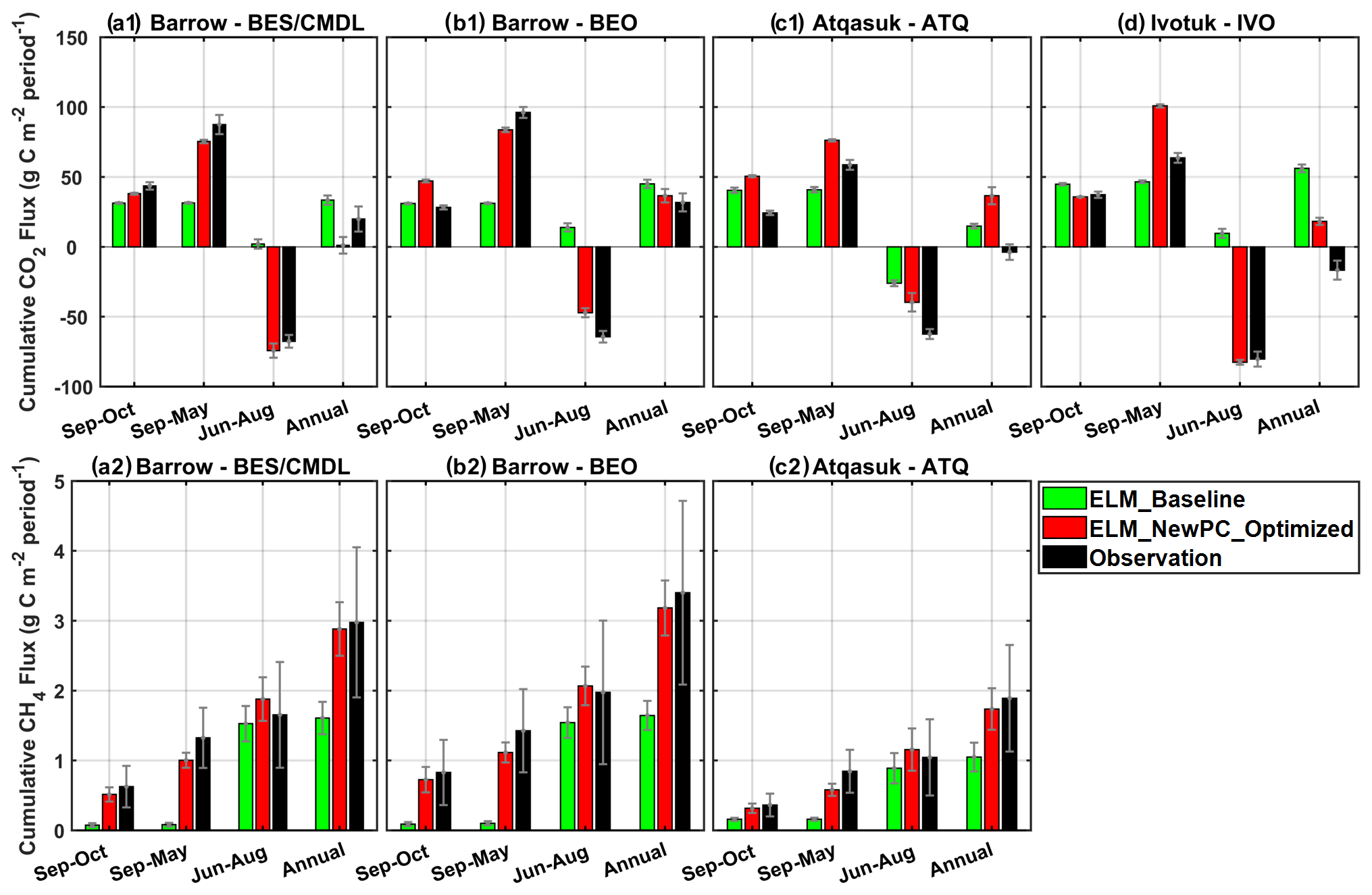
Figure 8Multi-year (2013–2017) averaged cumulative CH4 emissions (a2, b2, c2) and net CO2 flux (a1, b1, c1, d) during the early cold season (September and October), cold-season period (September to May), warm-season period (June to August), and the annual cycle (September to August) at our study sites. Due to the large discontinuity in CO2 observations, especially over the warm season (shown in Fig. 6), the observed annual CO2 budget is highly uncertain. Still, the cold-season contributions of both CH4 and CO2 emissions are greatly improved by the optimized ELMv1-ECA (i.e., ELM_NewPC_Optimized).
Table 4Total CH4 emissions and net CO2 flux over three seasonal periods, including the early cold season, cold season, and the warm season. “ELM_Optimized” here means ELM_NewPC_Optimized (Table 2). The percentage of each seasonal total CH4 emissions to the annual total is included in the brackets.

The optimized simulations showed larger improvements in cold-season CO2 emissions (Fig. 8; Table 4) for cold sites (i.e., BES/CMDL and BEO) than for the warmer site (i.e., ATQ and IVO). Specifically, compared to baseline results, the updated ELMv1-ECA reduced the biases in simulated cold-season CO2 emissions from −56.1 gC m−2 (64 % of the observation) to −12.1 gC m−2 (14 % of the observation) for BES/CMDL and from −65.0 gC m−2 (68 % of the observation) to −12.4 gC m−2 (13 % of the observation) for BEO. In contrast, the optimized simulation showed slight overestimations for cold-season CO2 emissions at ATQ and IVO (Table 4). Nevertheless, the optimized ELMv1-ECA provided greatly improved warm-season net CO2 flux for all the four sites, reducing biases by 110 %, 78 %, 37 %, and 102 % compared to baseline results at BES/CMDL, BEO, ATQ, and IVO, respectively. Indeed, the updated model switched warm-season net CO2 flux from baseline-simulated net emissions (positive net CO2 flux) to net uptake (negative net CO2 flux) at BES/CMDL, BEO, and IVO, correctly matching with observed warm-season net CO2 flux (Fig. 8).
The observed multi-year averaged annual net CO2 flux was 19.9 gC m−2 (source), 31.8 gC m−2 (source), −3.8 gC m−2 (sink), and −16.7 gC m−2 (sink) at BES/CMDL, BEO, ATQ, and IVO, respectively. However, due to the large discontinuity in CO2 observations (Fig. 6), the calculated annual CO2 budget is uncertain. Still, we can characterize the CO2 budget with simulated results using the updated ELMv1-ECA. We find that the simulated cold-season CO2 emissions were larger than the warm-season CO2 net uptake during the analyzing period (2013–2017) at all four sites (Fig. 8), showing annual net CO2 flux as 1.1 gC m−2 (source), 36.6 gC m−2 (source), 36.5 gC m−2 (source), and 18.2 gC m−2 (source) at BES/CMDL, BEO, ATQ, and IVO, respectively. The simulated CO2 emissions over the early cold season (September and October) accounted for 50 %, 56 %, 66 %, and 35 % of the total emissions throughout the cold season for BES/CMDL, BEO, ATQ, and IVO, respectively.
Through trend analysis between 1950 and 2017, we found that the ZCP durations showed increasing trends at all three sites, with ZCP trends increasing with depth (Table 6). At ATQ, a warmer site than BES/CMDL and BEO, the trends of ZCP durations increase from 0.12 to 0.49 d yr−1 along with the vertical soil profile. At BES/CMDL and BEO, only soil layers at 3 cm and 6 cm show statistically significant increasing trends, ranging from 0.10 to 0.13 d yr−1. The CO2 emissions during the 6 cm ZCP and during cold-season months (September to May) both showed increasing trends at all three sites (Table 6), ranging from 0.12 to 0.17 gC m−2 yr−1 for the 6 cm ZCP and from 0.30 to 0.40 gC m−2 yr−1 for the entire cold-season period. Annual CH4 emissions showed a nonsignificant increasing trend at ATQ with a rate of 0.52 mgC m−2 yr−1, but neither annual nor cold-season CH4 emissions show increasing trends at other sites. In the future, we will examine the generic model parameterization at more sites over the pan-Arctic; we will also optimize regional simulations against spatial datasets of CO2 and CH4 upscaled from in situ measurements over pan-Arctic permafrost domain (Natali et al., 2019; Virkkala et al., 2021; Zeng et al., 2020; Peltola et al., 2019) and discuss the uncertainty of estimated trends of the spatially averaged CO2 and CH4 emissions associated with snow impact and model parameterizations.
Table 5Historical trend of ZCP durations (days year−1) for each soil layer from 1950 to 2017. (Trends with p>0.05 are not statistically significant.)
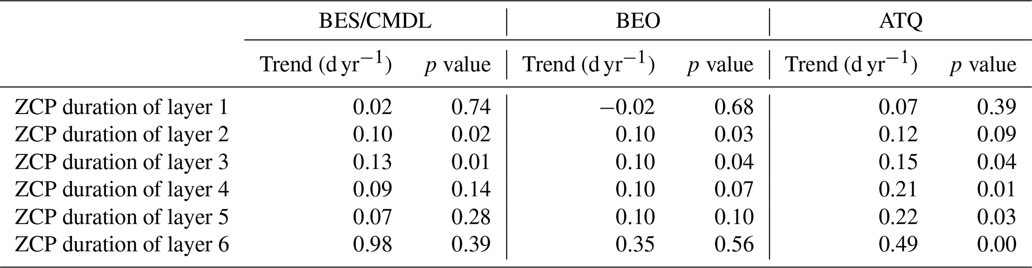
Table 6Historical trend (1950–2017) in site-scale heterotrophic respiration, CH4 emission, and CO2 flux during the ZCP duration at 6 cm (third layer), cold-season months (September–May), and the whole annual cycle (September–August). (Trends with p>0.05 are not statistically significant.)

In this study, we improved ELMv1-ECA simulated subsurface soil temperature, zero-curtain period durations, and cold-season CH4 and CO2 net emissions at Alaskan North Slope tundra sites. We first improved the numerical representation of coupled water and heat transport with freeze–thaw processes via modifying ELMv1-ECA's phase-change scheme. Then, we revised the dependency of soil decomposition rates on soil temperature and moisture. We further refined the cold-season methane processes by mimicking emission pathways through ice cracks and remnants of aerenchyma tissues, reducing the maximum oxidation rate constant, and reducing upper boundary (snow) resistance that allows CH4 to be emitted from frozen soils through snow to the atmosphere. We also used the updated ELMV1-ECA to estimate historical trends of cold-season CH4 and CO2 net emissions at the Alaskan tundra sites from 1950 to 2017. This study is among the first efforts toward improving simulations of zero-curtain periods and cold-season carbon emissions over the Arctic tundra by ESMs. The strategy of improving ELMv1-ECA phase-change scheme, environmental controls on microbial activity, and methane parameterizations can be easily applied to other global land models.
With the revised phase-change scheme, the updated ELMv1-ECA greatly improved site-scale simulations of soil temperature, soil moisture, and zero-curtain period. Specifically, the RMSE of daily subsurface soil temperature was substantially reduced compared to the baseline simulation, showing site-averaged improvements ranging from 58 % to 87 % over the early cold season (September to October) and from 36 % to 46 % over the annual cycle for soil layers within the active layer. The evaluation of simulated liquid water content with the new phase-change scheme, although limited by the availability of observations, showed a relative reduction in RMSE as high as 43 % for the fifth layer at ATQ and site-averaged improvements of 15 % and 21 % for the fourth and fifth layer, respectively. Simulated ZCP durations were also greatly improved, with, e.g., relative reductions in MAEs of 65 %, 65 %, 66 %, and 50 % for the fourth layer (about 12 cm) at BES/CMDL, BEO, ATQ, and IVO, respectively.
Based upon the improved simulations of soil temperature and moisture with the new phase-change scheme, the optimized parameterization for SOC decomposition scheme and the revised methane module, the site-averaged mean annual errors of cold-season emissions were reduced by 72 % and 70 % for CH4 and CO2, respectively. We also found that CH4 and CO2 emissions over the early cold season, i.e., September and October, which usually account for most of the zero-curtain period, contributed more than 50 % of the total emissions throughout the cold season (September to May). Zero-curtain period durations showed increasing trends from 1950 to 2017, with larger trends in deeper soil layers. Also, both CO2 emissions during the 6 cm depth zero-curtain period and the entire cold-season period (September to May) showed increasing trends. Note that the optimized parameterizations would be biased if there is a bias in simulated soil carbon and therefore should not be taken directly to other models without further analysis. Instead, the optimization procedure described in this study provides a roadmap that can be directly adopted to calibrate other models at different sites.
Although showing improvements compared to baseline results, the new simulations generally overestimated the contribution of the early-cold-season (September and October) CO2 emissions at BEO and ATQ. Many reasons could contribute to the overestimations, including poor representation of coupled biogeochemical and hydrological processes in the localized permafrost soil environment, the lack of accurate representation of inundated hydro-ecological dynamics, underestimation of snow accumulation due to micro-topographic effects, and thus the snow insulation to the ground (e.g., Bisht et al., 2018), among others. Strong microtopographic impacts on CO2 and CH4 emissions across seven landscape types in Barrow, Alaska, were recently reported (Wang et al., 2019; Grant et al., 2017a, b). Sensitivity analysis demonstrates large impacts of snow depth on simulated winter soil temperature, summer soil moisture, heterotrophic respiration, and CO2 fluxes (Fig. S9); therefore, the simulation of snow should be the subject of future investigations.
The underestimated emissions during post-ZCP months (October to November) may be caused by the lack of sudden bursts of CO2 and CH4 during the freeze-up period. In addition, the single static multiplicative function used to parameterize the impact of environmental conditions on respiration might not be appropriate because the environmental impact also depends on maximum respiration rate, soil texture, soil carbon content and quality, and microbial biomass (Tang and Riley, 2019). Moreover, due to lacking representations of wetland hydro-ecological dynamics, the model uses simulated upland heterotrophic respiration to estimate CH4 production (Riley et al., 2011), which might cause underestimations of CH4 emissions, especially under wet conditions. Also, inappropriately prescribed land cover at the site scale or inaccurate climate forcing (particularly air temperature and precipitation; Chang et al. 2019) could all impact snow accumulation processes (Tao et al., 2017), which can significantly impact CO2 and CH4 emission simulations. Customizing the complex local ecosystem vegetation community might be feasible at the site scale; however, it is less possible for regional or global land model simulations. This issue calls for the importance of upscaling methods to model (e.g., Pau et al., 2016; Liu et al., 2016) and measure (e.g., Natali et al., 2019; Virkkala et al., 2019) carbon and water cycle dynamics at the regional and global scales.
Given the persistent warming and the continued more severe warming in the cold season (Box et al., 2019), we envision continuing increases in cold-season CO2 and CH4 emissions from the permafrost tundra ecosystem. The increasing rate of cold-season heterotrophic respiration (releasing CO2) may become larger than the trend of warm-season vegetation CO2 uptake under future climate. To accurately characterize cold-season emissions and warm-season net uptake, models have to correctly simulate both components, which, however, few models can do. The updated ELMv1-ECA, with the enhanced capacity to reproduce cold-season CO2 and CH4 emissions proven by this study, can serve as a starting point to better predict permafrost carbon responses to future climate (Tao et al., 2021a). Finally, the complex water–carbon interactions require modeling systems with fully coupled hydrological–thermal–biogeochemical processes to better predict the carbon budget in permafrost regions under future climate.
ELMv1-ECA approximates the subsurface heat transfer process with a one-dimensional heat diffusion equation:
where T is the soil temperature (K), c is the volumetric soil heat capacity (J m−3 K−1), λ is soil thermal conductivity (W m−1 K−1), and z is the soil depth (m) of the ELMv1-ECA soil layers. The ELMv1-ECA soil column consists of 15 layers, with soil thickness increasing exponentially with depth. The bottom of soil column is down to 42 m, and the top 10 layers are hydrologically active with layer node depth as 0.0071, 0.0279, 0.0623, 0.1189, 0.2122, 0.3661, 0.6198, 1.0380, 1.7276, and 2.8646 m, respectively. The soil heat capacity and thermal conductivity is updated at each time step based on the fractions of soil matrix components, i.e., liquid water content, ice content, and soil solids. The impact of organic carbon on soil thermal and hydraulic properties was incorporated as a linear combination of the counterpart properties of mineral soil and organic matter (Lawrence and Slater, 2008). To solve the (Eq. A1), ELMv1-ECA employs the Crank–Nicolson method, resulting in a tridiagonal system equation (Oleson et al., 2013). We assume a zero-flux bottom boundary condition. The top boundary condition is estimated by solving the energy balance equation at the air and ground interface, with additionally an overlying five-layer snow model and a one-layer surface water model in between. When snow and surface water are present, ELMv1-ECA incorporates the snow layers and surface water layer into the tridiagonal system to solve the heat transfer along the entire column.
ELMv1-ECA incorporates freeze–thaw processes of soil water in a decoupled way. Specifically, the model determines the onset of thawing or freezing by soil temperature initially solved at time step n+1 without consideration of the phase-change process, denoted as , i.e.,
where Tf is the freezing temperature of water (0 ∘C in kelvin, i.e., 273.15 K), and are the mass of ice and liquid water (kg m−2) of layer i, and (kg m−2) is the supercooled liquid water that is allowed to coexist with ice given the subfreezing soil temperature . This varies with soil texture and temperature and is calculated by the freezing-point depression equation (Niu and Yang, 2006),
where Δzi is the soil thickness of the ith layer (in mm), θsat, i represents the soil porosity (i.e., the saturated volumetric water content), Lf is the latent heat of fusion (J kg−1), Bi is the Clapp and Hornberger exponent (Clapp and Hornberger, 1978), g is the gravitational acceleration (m s−2), and ψsat, i is the soil-texture-dependent saturated matric potential (mm).
The rate of phase change is initially assessed from the heat excess (or deficit) needed to change the estimated temperature to the freezing point. Specifically, the model first computes the energy (Hi) needed for adjusting current soil temperature () to Tf:
where , h is ground heat flux, and fsno and fh2osfc are the snow and surface water fraction within the grid cell, respectively. The mass change involved is then computed as (i.e., for soils below the top interface layer). That is, the mass of ice increased/decreased by freezing/melting is −Hm, releasing/absorbing energy Hi to bring up/down the current soil temperature to Tf. Accordingly, the ice and liquid mass are adjusted as
The Hi then is adjusted to , calculated as . The then is the ultimately determined latent heat and is used to further readjust soil temperature as in equation (Eq. A6),
in which the temperature adjusted to Tf is further increased by due to soil freezing since or decreased due to melting when .
To improve this scheme, we can incorporate soil water freezing phase change into equation (Eq. A1) and rewrite the heat transfer equation as (Eq. A7) or (Eq. A8),
where Lf is the latent heat of fusion (J kg−1), θliq is soil liquid water content (m3 m−3), and ρliq is the density of liquid water (kg m−3). To solve (Eq. A8), we need to compute the derivative of the soil freezing characteristic curve (θliq(T)) with respect to temperature (). As discussed above, we approximate the θliq(T) curve by combining the freezing-point temperature-depression equation (Fuchs et al., 1978) and the soil water retention curve (Clapp and Hornberger, 1978). This leads to the supercooled water formulation (Eq. A3) (Niu and Yang, 2006). Computing requires the soil freezing curves θliq(T) to be continuous and differentiable for a range of temperatures during the freezing process (Kurylyk and Watanabe, 2013; Hansson et al., 2004). Here, we follow the existing ELM framework discussed above to solve Eq. (A8). The original numerical representation for readjusting soil temperature (Eq. A6) obtained by the uncoupled two-step implementation (Eqs. A2 to A5) significantly overestimates soil water freezing rates. There are two reasons for the overestimation. First, the freezing point (Tf=0 ∘C) is used to determine the occurrence of soil water phase change under all conditions. To further freeze supercooled soil liquid water, however, the soil temperature has to be colder than a virtual soil temperature (as we described below). Second, due to the steep slope of (especially close to Tf=0 ∘C), the estimated ice mass increase (i.e., or ; see, Eq. A5) most often exceeds the required mass change, i.e., , and thus soil liquid water freezes quickly in a large chunk. Soon, the liquid water available to be frozen becomes too small to release sufficient latent heat to compensate for the required energy deficit ().
Thus, we revised the phase-change scheme mainly through incorporating a phase-change efficiency (ε) and replacing the constant freezing point Tf with the temperature of the freezing-point depression in Eq. (A2). The phase-change efficiency, introduced by Le Moigne et al. (2012) and adopted by Masson et al. (2013) and Yang et al. (2018a), is calculated as
where and is the soil liquid and ice volumetric water content of layer i at previous time step n, respectively, and θsat, i represents the soil porosity (i.e., the saturated volumetric water content). The temperature of the freezing-point depression, as a virtual temperature (Tv) reversely derived from the freezing-point temperature-depression equation, i.e., (Fuchs et al., 1978; Cary and Mayland, 1972), is calculated as
where Lf is the latent heat of fusion (J kg−1) and g is the gravitational acceleration (m s−2). is the soil water potential (mm), calculated as the soil water retention curve of Clapp and Hornberger (1978), i.e., , where as in Eq. (A3), Bi is the Clapp and Hornberger exponent, and ψsat, i is the soil-texture-dependent saturated matric potential (mm).
Then, through multiplying the initially estimated mass change (Hm) by the phase-change efficiency (ε), we replace the freezing point with an efficiency-weighted average of the initially solved soil temperature ( and the freezing point. Then, the updated soil temperature is expressed as
Here, is calculated by (Eq. A5) as well, but with updated Hm (i.e., ). The two changes can effectively improve the soil water freezing process simulations and prevent soil becoming irreversibly too cold quickly as simulated by the baseline phase-change scheme.
ELMv1-ECA explicitly simulates carbon cycle dynamics (both plant and soil) and accounts for the limitation of nutrient (i.e., nitrogen and phosphorus) availability for plant growth and the nutrient competition between plants and microbes (Burrows et al., 2020; Zhu et al., 2019; Golaz et al., 2019; Zhu et al., 2020). The ELMv1-ECA uses a century-like soil carbon decomposition cascade model with vertically resolved soil biogeochemistry (Koven et al., 2013b) and explicitly accounts for the influence of substrate and nutrient availability on soil respiration (both root and microbes) (Zhu et al., 2019).
Within the ELMv1-ECA century decomposition cascade model, the respiration fractions are parameterized as the fraction of the decomposition carbon flux out of each carbon pool, including litter and soil organic matter. The base decomposition rate is modified by a function representing environmental controls on soil decomposition, which accounts for the impacts of individual factors including temperature (fT) and moisture (fW), an oxygen scalar (fO), and a depth scalar (fD), in a multiplicative way, i.e., ftotal=fTfWfOfD.
We use a Q10-based standard exponential function to account for the temperature effect on decomposition,
where Q10=1.5 by default, which is consistent with ecosystem-level observations (Mahecha et al., 2010), and Tref is the reference temperature (25 ∘C). During cold seasons when soil temperature becomes subfreezing, respiration continues but with more controls from liquid water stress. The original moisture scalar (fW) within ELMV1-ECA is given in the formulation, calculated as
where is the soil water potential, and Bi is the Clapp and Hornberger exponent (Clapp and Hornberger, 1978). In frozen soil, the soil water potential is related to soil temperature through the freezing-point depression equation, i.e., (Fuchs et al., 1978; Cary and Mayland, 1972) in the supercooled water formulation (Niu and Yang, 2006). Thus, the liquid water stress on decomposition is translated into dependency on temperature when soil temperature is below the freezing point. By default, ψmin is −10 MPa, which predicts zero fW under frozen conditions since ψi under a subfreezing soil temperature easily gets smaller than −10 MPa (Fig. S1a). We thus reduced the ψmin to −103 and −106 MPa to alleviate the zero respiration problem in the frozen soils (see Fig. S1a). We also tested scalars documented by Sierra et al. (2015) and Yan et al. (2018) and included the full list in Table S2. ELMv1-ECA approximates oxygen stress (fO) as the ratio of available oxygen to that demanded by decomposers and has a minimum value of 0.2 (Oleson et al., 2013).
The depth scalar represents other unresolved depth-dependent processes (i.e., soil microbial dynamics, priming effects, etc.) (Koven et al., 2013b; Lawrence et al., 2015; Koven et al., 2015). Applying the depth scalar to decomposition rates would exponentially decrease the respiration fluxes along with the vertical soil layers. The Zτ is the e-folding depth for decomposition, and by default Zτ is 0.5 m (Oleson et al., 2013).
The ELMv1-ECA methane model includes the representations of CH4 production, oxidation, and three pathways of transport (i.e., aerenchyma tissues, ebullition, and aqueous and gaseous diffusion) and solves the transient reaction diffusion equation for CH4. ELMv1-ECA estimates CH4 production (P; mol m−3 s−1) in the anaerobic portion of the soil column based on the upland heterotrophic respiration (HR; mol C m−2 s−1) from soil and litter, further adjusted by factors representing influence from soil temperature (fT), pH (fpH), redox potential (fpE), and seasonal inundation condition (S) (Riley et al., 2011), expressed as
The is a fraction of anaerobically mineralized carbon atoms becoming CH4 and is 0.2 by default. Detailed explanation on these factors can be found in Riley et al. (2011). The methane production P is directly related to the estimated HR and impacted by soil temperature, and thus the changes in the carbon decomposition model (Appendix B) and water and heat transfer model (Appendix A) directly influence methane production simulations. Besides, ELMv1-ECA considers the availability of carbon substrate as an important driver of methanogenesis activity and methane production (Riley et al., 2011; Xu et al., 2016).
The ultimately estimated CH4 emissions are controlled by oxidation, transport mechanisms (i.e., aerenchyma transport, ebullition, and diffusion), and the upper boundary resistance. Detailed descriptions on CH4 oxidation and transport mechanisms are provided in Riley et al. (2011). Here we modified CH4 transport mechanisms for facilitating reasonable cold-season CH4 emissions.
Vascular plant aerenchyma tissues serve as diffusive pathways to transport CH4 from the soil to the atmosphere. The CH4 transport via aerenchyma from soil layer z (A(z), mol m−2 s−1) is calculated as
where C(z) and Ca are the gaseous CH4 concentrations (mol m−3) in soil depth z and in the atmosphere, respectively; ra is the aerodynamic resistance (s m−1); D is the gas diffusion coefficient (m2 s−1); p is aerenchyma porosity (–); rL is the ratio of root length to vertical depth (i.e., root obliquity); and ρr(z) is the root fraction in soil depth z (–). Taere is the specific aerenchyma area (m2 m−2) and is expressed as
where R represents the aerenchyma radius ( m); Na is the annual net primary production (NPP), and fN is the belowground fraction of current NPP; and the factor 0.22 represents average observed tiller biomass (gC per tiller) (Wania et al., 2010; Schimel, 1995). Here, tillers mean segmented stems of plants in the order of Poales, including grasses (Poaceae) and sedges (Cyperaceae) (Wania et al., 2010).
In ELMv1-ECA, methane emissions through aerenchyma were turned off when the soil temperature is below 0 ∘C. We first removed this temperature limitation; then, we integrated the emissions from ice cracks and remnants of aerenchyma tissues with Eq. (C3) by applying a small εaere during winter time. That is, when soil temperature is below the freezing point, where εaere represents possible ice crack fractions and remnants of aerenchyma tissues, and it is 0.01 by default. We also tested a larger value for this parameter together with and the maximum CH4 oxidation rate constant Ro, max (Table S3).
The Ro, max is a key variable controlling CH4 oxidation rate (Roxic), calculated as
where and are CH4 and O2 concentrations, respectively; and are the half-saturation coefficients (mol m−3) for and , respectively. Details about the CH4 oxidation are provided in Riley et al. (2011). The maximum oxidation rate Ro,max (mol m−3 s−1) by default is and for saturated and unsaturated conditions, respectively. We tested the Ro, max with the smaller value () for saturated condition as well (Table S3).
Another key variable that is highly uncertain is snow resistance to gas emissions. When snow is present, the upper boundary layer resistance to gas emissions is added by a snow resistance accounting for diffusion through the snow based on the Millington–Quirk expression (Riley et al. 2011). Specifically, the gaseous and aqueous diffusivity in snow is calculated by (Eq. C5)
where Dgas and Dliq are gaseous and aqueous diffusion coefficients (m2 s−1) for CH4, respectively (see Table 2 in Riley et al. 2011), εdiff is a scale factor (1 by default) for the diffusion coefficients, θwater is water-filled fraction of snow volume (–), and θair is air fraction in snow (–). The Dsnow is calculated for each snow layer; then, the total snow resistance is estimated as , where dz(i) is the thickness of ith snow layer. The top boundary layer conductance for CH4 then is calculated as , where Rpond is ponding resistance and Cg is ground conductance (details can be found in Oleson et al., 2013). We found the computed snow resistance generally was too large. We thus decreased snow resistance by introducing a new scale factor, i.e., εsnowdiff (102 by default), and replaced εdiff in Eq. (C5) with εsnowdiff to increase the conductance at the upper boundary when snow is present.
The observations used in this study are available at https://doi.org/10.3334/ornldaac/1300 (Zona et al., 2015) and https://doi.org/10.3334/ornldaac/1562 (Oechel and Kalhori, 2018). The UAF observations are available at http://permafrost.gi.alaska.edu (Permafrost Laboratory, 2021). This paper resulted in two updated versions of ELMv1-ECA, i.e., one optimized version from the discussion version (ELMv1a) and another version from the finalized paper (ELMv1b), which are all available at Zenodo (https://doi.org/10.5281/zenodo.5725525, Tao et al., 2021b).
The supplement related to this article is available online at: https://doi.org/10.5194/tc-15-5281-2021-supplement.
JT assembled observations, developed the methodology, conducted model simulations, analyzed results, and wrote and revised the paper. QZ and WJR contributed to the experiment design and to editing the original and revised manuscript. RBN edited the original and revised manuscript and provided valuable discussion and guidance.
The authors declare that they have no conflict of interest.
Publisher's note: Copernicus Publications remains neutral with regard to jurisdictional claims in published maps and institutional affiliations.
We are grateful for valuable discussions with Jinyun Tang, Roisin Commane, Xiyan Xu, Kai Yang, and Chenghai Wang. We thank the anonymous reviewers for their helpful comments.
This research has been supported by the U.S. Department of Energy, Office of Science, Office of Biological and Environmental Research (grant no. DE-SC0019063).
This paper was edited by Christian Beer and reviewed by two anonymous referees.
Anthony, K. M. W., Anthony, P., Grosse, G., and Chanton, J.: Geologic methane seeps along boundaries of Arctic permafrost thaw and melting glaciers, Nat. Geosci., 5, 419–426, 2012.
Arndt, K. A., Oechel, W. C., Goodrich, J. P., Bailey, B. A., Kalhori, A., Hashemi, J., Sweeney, C., and Zona, D.: Sensitivity of Methane Emissions to Later Soil Freezing in Arctic Tundra Ecosystems, J. Geophys. Res.-Biogeo., 124, 2595–2609, https://doi.org/10.1029/2019JG005242, 2019.
Belshe, E. F., Schuur, E. A. G., and Bolker, B. M.: Tundra ecosystems observed to be CO2 sources due to differential amplification of the carbon cycle, Ecol. Lett., 16, 1307–1315, https://doi.org/10.1111/ele.12164, 2013.
Bhanja, S. N. and Wang, J. Y.: Estimating influences of environmental drivers on soil heterotrophic respiration in the Athabasca River Basin, Canada, Environ. Pollut., 257, https://doi.org/10.1016/j.envpol.2019.113630, 2020.
Bisht, G., Riley, W. J., Wainwright, H. M., Dafflon, B., Yuan, F., and Romanovsky, V. E.: Impacts of microtopographic snow redistribution and lateral subsurface processes on hydrologic and thermal states in an Arctic polygonal ground ecosystem: a case study using ELM-3D v1.0, Geosci. Model Dev., 11, 61–76, https://doi.org/10.5194/gmd-11-61-2018, 2018.
Box, J. E., Colgan, W. T., Christensen, T. R., Schmidt, N. M., Lund, M., Parmentier, F. J. W., Brown, R., Bhatt, U. S., Euskirchen, E. S., Romanovsky, V. E., Walsh, J. E., Overland, J. E., Wang, M. Y., Corell, R. W., Meier, W. N., Wouters, B., Mernild, S., Mard, J., Pawlak, J., and Olsen, M. S.: Key indicators of Arctic climate change: 1971–2017, Environ. Res. Lett., 14, 045010, https://doi.org/10.1088/1748-9326/aafc1b, 2019.
Burrows, S. M., Maltrud, M., Yang, X., Zhu, Q., Jeffery, N., Shi, X., Ricciuto, D., Wang, S., Bisht, G., Tang, J., Wolfe, J., Harrop, B. E., Singh, B., Brent, L., Baldwin, S., Zhou, T., Cameron-Smith, P., Keen, N., Collier, N., Xu, M., Hunke, E. C., Elliott, S. M., Turner, A. K., Li, H., Wang, H., Golaz, J. C., Bond-Lamberty, B., Hoffman, F. M., Riley, W. J., Thornton, P. E., Calvin, K., and Leung, L. R.: The DOE E3SM v1.1 Biogeochemistry Configuration: Description and Simulated Ecosystem-Climate Responses to Historical Changes in Forcing, J. Adv. Model. Earth. Sy., 12, e2019MS001766, https://doi.org/10.1029/2019MS001766, 2020.
Cary, J. W. and Mayland, H. F.: Salt and Water Movement in Unsaturated Frozen Soil, Soil. Sci. Soc. Am. Pro., 36, 549–555, 1972.
Chadburn, S. E., Aalto, T., Aurela, M., Baldocchi, D., Biasi, C., Boike, J., Burke, E. J., Comyn-Platt, E., Dolman, A. J., Duran-Rojas, C., Fan, Y. C., Friborg, T., Gao, Y., Gedney, N., Gockede, M., Hayman, G. D., Holl, D., Hugelius, G., Kutzbach, L., Lee, H., Lohila, A., Parmentier, F. J. W., Sachs, T., Shurpali, N. J., and Westermann, S.: Modeled Microbial Dynamics Explain the Apparent Temperature Sensitivity of Wetland Methane Emissions, Global Biogeochem. Cy., 34, e2020GB006678, https://doi.org/10.1029/2020GB006678, 2020.
Chang, K.-Y., Riley, W. J., Crill, P. M., Grant, R. F., Rich, V. I., and Saleska, S. R.: Large carbon cycle sensitivities to climate across a permafrost thaw gradient in subarctic Sweden, The Cryosphere, 13, 647–663, https://doi.org/10.5194/tc-13-647-2019, 2019.
Chang, K.-Y., Riley, W. J., Crill, P. M., Grant, R. F., and Saleska, S. R.: Hysteretic temperature sensitivity of wetland CH4 fluxes explained by substrate availability and microbial activity, Biogeosciences, 17, 5849–5860, https://doi.org/10.5194/bg-17-5849-2020, 2020.
Chang, K. Y., Riley, W. J., Knox, S. H., et al.: Substantial hysteresis in emergent temperature sensitivity of global wetland CH4 emissions, Nat. Commun., 12, 2266, https://doi.org/10.1038/s41467-021-22452-1, 2021.
Clapp, R. B. and Hornberger, G. M.: Empirical equations for some soil hydraulic properties, Water Resour. Res., 14, 601–604, 1978.
Commane, R., Lindaas, J., Benmergui, J., Luus, K. A., Chang, R. Y. W., Daube, B. C., Euskirchen, E. S., Henderson, J. M., Karion, A., Miller, J. B., Miller, S. M., Parazoo, N. C., Randerson, J. T., Sweeney, C., Tans, P., Thoning, K., Veraverbeke, S., Miller, C. E., and Wofsy, S. C.: Carbon dioxide sources from Alaska driven by increasing early winter respiration from Arctic tundra, P. Natl. Acad. Sci. USA, 114, 5361–5366, 2017.
Dankers, R., Burke, E. J., and Price, J.: Simulation of permafrost and seasonal thaw depth in the JULES land surface scheme, The Cryosphere, 5, 773–790, https://doi.org/10.5194/tc-5-773-2011, 2011.
Davidson, E. A. and Janssens, I. A.: Temperature sensitivity of soil carbon decomposition and feedbacks to climate change, Nature, 440, 165–173, 2006.
Davidson, S. J. and Zona, D.: Arctic Vegetation Plots in Flux Tower Footprints, North Slope, Alaska, 2014, ORNL DAAC, Oak Ridge, Tennessee, USA, https://doi.org/10.3334/ORNLDAAC/1546, 2018.
Delwiche, K. B., Knox, S. H., Malhotra, A., Fluet-Chouinard, E., McNicol, G., Feron, S., Ouyang, Z., Papale, D., Trotta, C., Canfora, E., Cheah, Y.-W., Christianson, D., Alberto, Ma. C. R., Alekseychik, P., Aurela, M., Baldocchi, D., Bansal, S., Billesbach, D. P., Bohrer, G., Bracho, R., Buchmann, N., Campbell, D. I., Celis, G., Chen, J., Chen, W., Chu, H., Dalmagro, H. J., Dengel, S., Desai, A. R., Detto, M., Dolman, H., Eichelmann, E., Euskirchen, E., Famulari, D., Fuchs, K., Goeckede, M., Gogo, S., Gondwe, M. J., Goodrich, J. P., Gottschalk, P., Graham, S. L., Heimann, M., Helbig, M., Helfter, C., Hemes, K. S., Hirano, T., Hollinger, D., Hörtnagl, L., Iwata, H., Jacotot, A., Jurasinski, G., Kang, M., Kasak, K., King, J., Klatt, J., Koebsch, F., Krauss, K. W., Lai, D. Y. F., Lohila, A., Mammarella, I., Belelli Marchesini, L., Manca, G., Matthes, J. H., Maximov, T., Merbold, L., Mitra, B., Morin, T. H., Nemitz, E., Nilsson, M. B., Niu, S., Oechel, W. C., Oikawa, P. Y., Ono, K., Peichl, M., Peltola, O., Reba, M. L., Richardson, A. D., Riley, W., Runkle, B. R. K., Ryu, Y., Sachs, T., Sakabe, A., Sanchez, C. R., Schuur, E. A., Schäfer, K. V. R., Sonnentag, O., Sparks, J. P., Stuart-Haëntjens, E., Sturtevant, C., Sullivan, R. C., Szutu, D. J., Thom, J. E., Torn, M. S., Tuittila, E.-S., Turner, J., Ueyama, M., Valach, A. C., Vargas, R., Varlagin, A., Vazquez-Lule, A., Verfaillie, J. G., Vesala, T., Vourlitis, G. L., Ward, E. J., Wille, C., Wohlfahrt, G., Wong, G. X., Zhang, Z., Zona, D., Windham-Myers, L., Poulter, B., and Jackson, R. B.: FLUXNET-CH4: a global, multi-ecosystem dataset and analysis of methane seasonality from freshwater wetlands, Earth Syst. Sci. Data, 13, 3607–3689, https://doi.org/10.5194/essd-13-3607-2021, 2021.
Etiope, G. and Klusman, R. W.: Microseepage in drylands: Flux and implications in the global atmospheric source/sink budget of methane, Global Planet. Change, 72, 265–274, 2010.
Fahnestock, J. T., Jones, M. H., Brooks, P. D., Walker, D. A., and Welker, J. M.: Winter and early spring CO2 efflux from tundra communities of northern Alaska, J. Geophys. Res.-Atmos., 103, 29023–29027, https://doi.org/10.1029/98jd00805, 1998.
Fuchs, M., Campbell, G., and Papendick, R.: An analysis of sensible and latent heat flow in a partially frozen unsaturated soil, Soil Sci. Soc. Am. J., 42, 379–385, 1978.
Golaz, J. C., Caldwell, P. M., Van Roekel, L. P., Petersen, M. R., Tang, Q., Wolfe, J. D., Abeshu, G., Anantharaj, V., Asay-Davis, X. S., Bader, D. C., Baldwin, S. A., Bisht, G., Bogenschutz, P. A., Branstetter, M., Brunke, M. A., Brus, S. R., Burrows, S. M., Cameron-Smith, P. J., Donahue, A. S., Deakin, M., Easter, R. C., Evans, K. J., Feng, Y., Flanner, M., Foucar, J. G., Fyke, J. G., Griffin, B. M., Hannay, C., Harrop, B. E., Hoffman, M. J., Hunke, E. C., Jacob, R. L., Jacobsen, D. W., Jeffery, N., Jones, P. W., Keen, N. D., Klein, S. A., Larson, V. E., Leung, L. R., Li, H. Y., Lin, W. Y., Lipscomb, W. H., Ma, P. L., Mahajan, S., Maltrud, M. E., Mametjanov, A., McClean, J. L., McCoy, R. B., Neale, R. B., Price, S. F., Qian, Y., Rasch, P. J., Eyre, J. E. J. R., Riley, W. J., Ringler, T. D., Roberts, A. F., Roesler, E. L., Salinger, A. G., Shaheen, Z., Shi, X. Y., Singh, B., Tang, J. Y., Taylor, M. A., Thornton, P. E., Turner, A. K., Veneziani, M., Wan, H., Wang, H. L., Wang, S. L., Williams, D. N., Wolfram, P. J., Worley, P. H., Xie, S. C., Yang, Y., Yoon, J. H., Zelinka, M. D., Zender, C. S., Zeng, X. B., Zhang, C. Z., Zhang, K., Zhang, Y., Zheng, X., Zhou, T., and Zhu, Q.: The DOE E3SM Coupled Model Version 1: Overview and Evaluation at Standard Resolution, J. Adv. Model. Earth Sy., 11, 2089–2129, 2019.
Graf, A., Weihermuller, L., Huisman, J. A., Herbst, M., and Vereecken, H.: Comment on “Global Convergence in the Temperature Sensitivity of Respiration at Ecosystem Level”, Science, 331, 1265, https://doi.org/10.1126/science.1196948, 2011.
Grant, R. F., Mekonnen, Z. A., Riley, W. J., Arora, B., and Torn, M. S.: Mathematical Modelling of Arctic Polygonal Tundra with Ecosys: 2. Microtopography Determines How CO2 and CH4 Exchange Responds to Changes in Temperature and Precipitation, J. Geophys. Res.-Biogeo., 122, 3174–3187, 2017a.
Grant, R. F., Mekonnen, Z. A., Riley, W. J., Wainwright, H. M., Graham, D., and Torn, M. S.: Mathematical Modelling of Arctic Polygonal Tundra with Ecosys: 1. Microtopography Determines How Active Layer Depths Respond to Changes in Temperature and Precipitation, J. Geophys. Res.-Biogeo., 122, 3161–3173, 2017b.
Hansson, K., Simunek, J., Mizoguchi, M., Lundin, L. C., and van Genuchten, M. T.: Water flow and heat transport in frozen soil: Numerical solution and freeze-thaw applications, Vadose Zone J., 3, 693–704, 2004.
Harmon, M. and Domingo, J.: A users guide to STANDCARB version 2.0: a model to simulate the carbon stores in forest stands, Dep. of For. Sci., Oreg. State Univ., Corvallis, OR, USA, 2001.
Harris, I.: CRU JRA v1. 1: A forcings dataset of gridded land surface blend of Climatic Research Unit (CRU) and Japanese reanalysis (JRA) data; January 1901–December 2017, University of East Anglia Climatic Research Unit, Centre for Environmental Data Analysis, 2905, Norwich NR4 7TJ, United Kingdom, https://doi.org/10.5285/13f3635174794bb98cf8ac4b0ee8f4ed, 2019.
Jones, M. H., Fahnestock, J. T., and Welker, J. M.: Early and late winter CO2 efflux from arctic tundra in the Kuparuk River watershed, Alaska, USA, Arct. Antarct. Alp. Res., 31, 187–190, https://doi.org/10.2307/1552607, 1999.
Kelly, R., Parton, W., Hartman, M., Stretch, L., Ojima, D., and Schimel, D.: Intra-annual and interannual variability of ecosystem processes in shortgrass steppe, J. Geophys. Res.-Atmos., 105, 20093–20100, 2000.
Kim, D., Lee, M. I., and Seo, E.: Improvement of Soil Respiration Parameterization in a Dynamic Global Vegetation Model and Its Impact on the Simulation of Terrestrial Carbon Fluxes, J. Climate, 32, 127–143, 2019.
Kim, Y., Ueyama, M., Nakagawa, F., Tsunogai, U., Harazono, Y., and Tanaka, N.: Assessment of winter fluxes of CO2 and CH4 in boreal forest soils of central Alaska estimated by the profile method and the chamber method: a diagnosis of methane emission and implications for the regional carbon budget, Tellus B, 59, 223–233, 2007.
Kittler, F., Heimann, M., Kolle, O., Zimov, N., Zimov, S., and Gockede, M.: Long-Term Drainage Reduces CO2 Uptake and CH4 Emissions in a Siberian Permafrost Ecosystem, Global Biogeochem. Cy., 31, 1704–1717, 2017.
Knox, S. H., Jackson, R. B., Poulter, B., McNicol, G., Fluet-Chouinard, E., Zhang, Z., Hugelius, G., Bousquet, P., Canadell, J. G., Saunois, M., Papale, D., Chu, H., Keenan, T. F., Baldocchi, D., Torn, M. S., Mammarella, I., Trotta, C., Aurela, M., Bohrer, G., Campbell, D. I., Cescatti, A., Chamberlain, S., Chen, J., Chen, W., Dengel, S., Desai, A. R., Euskirchen, E., Friborg, T., Gasbarra, D., Goded, I., Goeckede, M., Heimann, M., Helbig, M., Hirano, T., Hollinger, D. Y., Iwata, H., Kang, M., Klatt, J., Krauss, K. W., Kutzbach, L., Lohila, A., Mitra, B., Morin, T. H., Nilsson, M. B., Niu, S., Noormets, A., Oechel, W. C., Peichl, M., Peltola, O., Reba, M. L., Richardson, A. D., Runkle, B. R. K., Ryu, Y., Sachs, T., Schafer, K. V. R., Schmid, H. P., Shurpali, N., Sonnentag, O., Tang, A. C. I., Ueyama, M., Vargas, R., Vesala, T., Ward, E. J., Windham-Myers, L., Wohlfahrt, G., and Zona, D.: FLUXNET-CH4 Synthesis Activity: Objectives, Observations, and Future Directions, B. Am. Meteorol. Soc., 100, 2607–2632, https://doi.org/10.1175/Bams-D-18-0268.1, 2019.
Koven, C. D., Ringeval, B., Friedlingstein, P., Ciais, P., Cadule, P., Khvorostyanov, D., Krinner, G., and Tarnocai, C.: Permafrost carbon-climate feedbacks accelerate global warming, P. Natl. Acad. Sci. USA, 108, 14769–14774, 2011.
Koven, C. D., Riley, W. J., and Stern, A.: Analysis of Permafrost Thermal Dynamics and Response to Climate Change in the CMIP5 Earth System Models, J. Climate, 26, 1877–1900, https://doi.org/10.1175/Jcli-D-12-00228.1, 2013a.
Koven, C. D., Riley, W. J., Subin, Z. M., Tang, J. Y., Torn, M. S., Collins, W. D., Bonan, G. B., Lawrence, D. M., and Swenson, S. C.: The effect of vertically resolved soil biogeochemistry and alternate soil C and N models on C dynamics of CLM4, Biogeosciences, 10, 7109–7131, https://doi.org/10.5194/bg-10-7109-2013, 2013b.
Koven, C. D., Lawrence, D. M., and Riley, W. J.: Permafrost carbon-climate feedback is sensitive to deep soil carbon decomposability but not deep soil nitrogen dynamics, P. Natl. Acad. Sci. USA, 112, 3752–3757, https://doi.org/10.1073/pnas.1415123112, 2015.
Koven, C. D., Hugelius, G., Lawrence, D. M., and Wieder, W. R.: Higher climatological temperature sensitivity of soil carbon in cold than warm climates, Nat. Clim. Change, 7, 817–822, https://doi.org/10.1038/Nclimate3421, 2017.
Kuhn, M. A., Varner, R. K., Bastviken, D., Crill, P., MacIntyre, S., Turetsky, M., Walter Anthony, K., McGuire, A. D., and Olefeldt, D.: BAWLD-CH4: a comprehensive dataset of methane fluxes from boreal and arctic ecosystems, Earth Syst. Sci. Data, 13, 5151–5189, https://doi.org/10.5194/essd-13-5151-2021, 2021.
Kurylyk, B. L. and Watanabe, K.: The mathematical representation of freezing and thawing processes in variably-saturated, non-deformable soils, Adv. Water Resour., 60, 160–177, https://doi.org/10.1016/j.advwatres.2013.07.016, 2013.
Kurylyk, B. L. and Hayashi, M.: Improved Stefan Equation Correction Factors to Accommodate Sensible Heat Storage during Soil Freezing or Thawing, Permafrost Periglac., 27, 189–203, 2016.
Lawrence, D. M., Thornton, P. E., Oleson, K. W., and Bonan, G. B.: The partitioning of evapotranspiration into transpiration, soil evaporation, and canopy evaporation in a GCM: Impacts on land-atmosphere interaction, J. Hydrometeorol., 8, 862–880, 2007.
Lawrence, D. M. and Slater, A. G.: Incorporating organic soil into a global climate model, Clim. Dynam., 30, 145–160, https://doi.org/10.1007/s00382-007-0278-1, 2008.
Lawrence, D. M. and Slater, A. G.: The contribution of snow condition trends to future ground climate, Clim. Dynam., 34, 969–981, 2010.
Lawrence, D. M., Koven, C. D., Swenson, S. C., Riley, W. J., and Slater, A. G.: Permafrost thaw and resulting soil moisture changes regulate projected high-latitude CO2 and CH4 emissions, Environ. Res. Lett., 10, 094011, https://doi.org/10.1088/1748-9326/10/9/094011, 2015.
Le Moigne, P., Boone, A., Belamari, S., Brun, E., Calvet, J., Decharme, B., Faroux, S., Gibelin, A., Giordani, H., Lafont, S., Lebeaupin, C., Le Moigne, P., Mahfouf, J., Martin, E., Masson, V., Mironov, D., Morin, S., Noilhan, J., Tulet, P., Van den Hurk, B., and Vionnet, V.: SURFEX Scientific Documentation, Note de centre (CNRM/GMME), Météo-France, Toulouse, France, 2012.
Liu, Y. N., Bisht, G., Subin, Z. M., Riley, W. J., and Pau, G. S. H.: A Hybrid Reduced-Order Model of Fine-Resolution Hydrologic Simulations at a Polygonal Tundra Site, Vadose Zone. J., 15, vzj2015.05.0068, https://doi.org/10.2136/vzj2015.05.0068, 2016.
Lyman, S. N., Tran, H. N., Mansfield, M. L., Bowers, R., and Smith, A.: Strong temporal variability in methane fluxes from natural gas well pad soils, Atmo. Poll. Res., 11, 1386–1395, https://doi.org/10.1016/j.apr.2020.05.011, 2020.
Mahecha, M. D., Reichstein, M., Carvalhais, N., Lasslop, G., Lange, H., Seneviratne, S. I., Vargas, R., Ammann, C., Arain, M. A., Cescatti, A., Janssens, I. A., Migliavacca, M., Montagnani, L., and Richardson, A. D.: Global Convergence in the Temperature Sensitivity of Respiration at Ecosystem Level, Science, 329, 838–840, 2010.
Masson, V., Le Moigne, P., Martin, E., Faroux, S., Alias, A., Alkama, R., Belamari, S., Barbu, A., Boone, A., Bouyssel, F., Brousseau, P., Brun, E., Calvet, J.-C., Carrer, D., Decharme, B., Delire, C., Donier, S., Essaouini, K., Gibelin, A.-L., Giordani, H., Habets, F., Jidane, M., Kerdraon, G., Kourzeneva, E., Lafaysse, M., Lafont, S., Lebeaupin Brossier, C., Lemonsu, A., Mahfouf, J.-F., Marguinaud, P., Mokhtari, M., Morin, S., Pigeon, G., Salgado, R., Seity, Y., Taillefer, F., Tanguy, G., Tulet, P., Vincendon, B., Vionnet, V., and Voldoire, A.: The SURFEXv7.2 land and ocean surface platform for coupled or offline simulation of earth surface variables and fluxes, Geosci. Model Dev., 6, 929–960, https://doi.org/10.5194/gmd-6-929-2013, 2013.
Mekonnen, Z. A., Riley, W. J., Grant, R. F., and Romanovsky, V.: Changes in precipitation and air temperature contribute comparably to permafrost degradation in a warmer climate, Environ. Res. Lett., 16, 024008, https://doi.org/10.1088/1748-9326/abc444, 2020.
Meyer, N., Welp, G., and Amelung, W.: The Temperature Sensitivity (Q10) of Soil Respiration: Controlling Factors and Spatial Prediction at Regional Scale Based on Environmental Soil Classes, Global Biogeochem. Cy., 32, 306–323, 2018.
Moriasi, D. N., Arnold, J. G., Van Liew, M. W., Bingner, R. L., Harmel, R. D., and Veith, T. L.: Model evaluation guidelines for systematic quantification of accuracy in watershed simulations, T. Asabe, 50, 885–900, 2007.
Moyano, F. E., Manzoni, S., and Chenu, C.: Responses of soil heterotrophic respiration to moisture availability: An exploration of processes and models, Soil Biol. Biochem., 59, 72–85, 2013.
Nash, J. E. and Sutcliffe, J. V.: River flow forecasting through conceptual models part I – A discussion of principles, J. Hydrol., 10, 282–290, https://doi.org/10.1016/0022-1694(70)90255-6, 1970.
Natali, S. M., Watts, J. D., Rogers, B. M., Potter, S., Ludwig, S. M., Selbmann, A.-K., Sullivan, P. F., Abbott, B. W., Arndt, K. A., Birch, L., Björkman, M. P., Bloom, A. A., Celis, G., Christensen, T. R., Christiansen, C. T., Commane, R., Cooper, E. J., Crill, P., Czimczik, C., Davydov, S., Du, J., Egan, J. E., Elberling, B., Euskirchen, E. S., Friborg, T., Genet, H., Göckede, M., Goodrich, J. P., Grogan, P., Helbig, M., Jafarov, E. E., Jastrow, J. D., Kalhori, A. A. M., Kim, Y., Kimball, J. S., Kutzbach, L., Lara, M. J., Larsen, K. S., Lee, B.-Y., Liu, Z., Loranty, M. M., Lund, M., Lupascu, M., Madani, N., Malhotra, A., Matamala, R., McFarland, J., McGuire, A. D., Michelsen, A., Minions, C., Oechel, W. C., Olefeldt, D., Parmentier, F.-J. W., Pirk, N., Poulter, B., Quinton, W., Rezanezhad, F., Risk, D., Sachs, T., Schaefer, K., Schmidt, N. M., Schuur, E. A. G., Semenchuk, P. R., Shaver, G., Sonnentag, O., Starr, G., Treat, C. C., Waldrop, M. P., Wang, Y., Welker, J., Wille, C., Xu, X., Zhang, Z., Zhuang, Q., and Zona, D.: Large loss of CO2 in winter observed across the northern permafrost region, Nat. Clim. Change, 9, 852–857, https://doi.org/10.1038/s41558-019-0592-8, 2019.
Neumann, R. B., Moorberg, C. J., Lundquist, J. D., Turner, J. C., Waldrop, M. P., McFarland, J. W., Euskirchen, E. S., Edgar, C. W., and Turetsky, M. R.: Warming effects of spring rainfall increase methane emissions from thawing permafrost, Geophys. Res. Lett., 46, 1393–1401, https://doi.org/10.1029/2018GL081274, 2019.
Nicolsky, D. J., Romanovsky, V. E., Alexeev, V. A., and Lawrence, D. M.: Improved modeling of permafrost dynamics in a GCM land-surface scheme, Geophys. Res. Lett., 34, L08501, https://doi.org/10.1029/2007GL029525, 2007.
Niu, G. Y., and Yang, Z. L.: Effects of frozen soil on snowmelt runoff and soil water storage at a continental scale, J. Hydrometeorol., 7, 937–952, 2006.
Oechel, W. C., Vourlitis, G. L., Hastings, S. J., Zulueta, R. C., Hinzman, L., and Kane, D.: Acclimation of ecosystem CO2 exchange in the Alaskan Arctic in response to decadal climate warming, Nature, 406, 978–981, 2000.
Oechel, W. C., Laskowski, C. A., Burba, G., Gioli, B., and Kalhori, A. A. M.: Annual patterns and budget of CO2 flux in an Arctic tussock tundra ecosystem, J. Geophys. Res.-Biogeo., 119, 323–339, 2014.
Oechel, W. C. and Kalhori, A.: ABoVE: CO2 and CH4 Fluxes and Meteorology at Flux Tower Sites, Alaska, 2015–2017, ORNL DAAC, Oak Ridge, Tennessee, USA, https://doi.org/10.3334/ornldaac/1562, 2018.
Oleson, K. W., Lawrence, D., Bonan, G., Drewniak, B., Huang, M., Koven, C., Levis, S., Li, F., Riley, W., and Subin, Z.: Technical Description of version 4.5 of the Community Land Model (CLM)(NCAR Technical Note No. NCAR/TN-503+ STR), Citeseer, National Center for Atmospheric Research, PO Box, 3000, Boulder, Colorado, USA, 2013.
Outcalt, S. I., Nelson, F. E., and Hinkel, K. M.: The Zero-Curtain Effect – Heat and Mass-Transfer across an Isothermal Region in Freezing Soil, Water Resour. Res., 26, 1509–1516, 1990.
Permafrost Laboratory: The UAF observations, available at: http://permafrost.gi.alaska.edu, last access: 19 November 2021.
Pau, G. S. H., Shen, C. P., Riley, W. J., and Liu, Y. N.: Accurate and efficient prediction of fine-resolution hydrologic and carbon dynamic simulations from coarse-resolution models, Water Resour. Res., 52, 791–812, 2016.
Peltola, O., Vesala, T., Gao, Y., Räty, O., Alekseychik, P., Aurela, M., Chojnicki, B., Desai, A. R., Dolman, A. J., Euskirchen, E. S., Friborg, T., Göckede, M., Helbig, M., Humphreys, E., Jackson, R. B., Jocher, G., Joos, F., Klatt, J., Knox, S. H., Kowalska, N., Kutzbach, L., Lienert, S., Lohila, A., Mammarella, I., Nadeau, D. F., Nilsson, M. B., Oechel, W. C., Peichl, M., Pypker, T., Quinton, W., Rinne, J., Sachs, T., Samson, M., Schmid, H. P., Sonnentag, O., Wille, C., Zona, D., and Aalto, T.: Monthly gridded data product of northern wetland methane emissions based on upscaling eddy covariance observations, Earth Syst. Sci. Data, 11, 1263–1289, https://doi.org/10.5194/essd-11-1263-2019, 2019.
Piao, S. L., Ciais, P., Friedlingstein, P., Peylin, P., Reichstein, M., Luyssaert, S., Margolis, H., Fang, J. Y., Barr, A., Chen, A. P., Grelle, A., Hollinger, D. Y., Laurila, T., Lindroth, A., Richardson, A. D., and Vesala, T.: Net carbon dioxide losses of northern ecosystems in response to autumn warming, Nature, 451, 49–52, 2008.
Rafique, R., Xia, J., Hararuk, O., Asrar, G. R., Leng, G., Wang, Y., and Luo, Y.: Divergent predictions of carbon storage between two global land models: attribution of the causes through traceability analysis, Earth Syst. Dynam., 7, 649–658, https://doi.org/10.5194/esd-7-649-2016, 2016.
Riley, W. J., Subin, Z. M., Lawrence, D. M., Swenson, S. C., Torn, M. S., Meng, L., Mahowald, N. M., and Hess, P.: Barriers to predicting changes in global terrestrial methane fluxes: analyses using CLM4Me, a methane biogeochemistry model integrated in CESM, Biogeosciences, 8, 1925–1953, https://doi.org/10.5194/bg-8-1925-2011, 2011.
Romanovsky, V. E., Kholodov, A. L., Cable, W. L., Cohen, L., Panda, S., Marchenko, S., Muskett, R. R., and Nicolsky, D.: Network of Permafrost Observatories in North America and Russia, NSF Arctic Data Center, https://doi.org/10.18739/A2SH27, 2009.
Russell, S. J., Bohrer, G., Johnson, D. R., Villa, J. A., Heltzel, R., Rey-Sanchez, C., and Matthes, J. H.: Quantifying CH4 concentration spikes above baseline and attributing CH4 sources to hydraulic fracturing activities by continuous monitoring at an off-site tower, Atmos. Environ., 228, 117452, https://doi.org/10.1016/j.atmosenv.2020.117452, 2020.
Sapriza-Azuri, G., Gamazo, P., Razavi, S., and Wheater, H. S.: On the appropriate definition of soil profile configuration and initial conditions for land surface–hydrology models in cold regions, Hydrol. Earth Syst. Sci., 22, 3295–3309, https://doi.org/10.5194/hess-22-3295-2018, 2018.
Schimel, J. P.: Plant-Transport and Methane Production as Controls on Methane Flux from Arctic Wet Meadow Tundra, Biogeochemistry, 28, 183–200, 1995.
Sierra, C. A., Trumbore, S. E., Davidson, E. A., Vicca, S., and Janssens, I.: Sensitivity of decomposition rates of soil organic matter with respect to simultaneous changes in temperature and moisture, J. Adv. Model Earth Sy, 7, 335–356, 2015.
Sierra, C. A., Malghani, S., and Loescher, H. W.: Interactions among temperature, moisture, and oxygen concentrations in controlling decomposition rates in a boreal forest soil, Biogeosciences, 14, 703–710, https://doi.org/10.5194/bg-14-703-2017, 2017.
Skopp, J., Jawson, M., and Doran, J.: Steady-state aerobic microbial activity as a function of soil water content, Soil Sci. Soc. Am. J., 54, 1619–1625, 1990.
Slater, A. G., Lawrence, D. M., and Koven, C. D.: Process-level model evaluation: a snow and heat transfer metric, The Cryosphere, 11, 989–996, https://doi.org/10.5194/tc-11-989-2017, 2017.
Tang, J. Y. and Riley, W. J.: Weaker soil carbon-climate feedbacks resulting from microbial and abiotic interactions, Nat. Clim. Change, 5, 56–60, https://doi.org/10.1038/Nclimate2438, 2015.
Tang, J. Y. and Riley, W. J.: A Theory of Effective Microbial Substrate Affinity Parameters in Variably Saturated Soils and an Example Application to Aerobic Soil Heterotrophic Respiration, J. Geophys. Res.-Biogeo., 124, 918–940, 2019.
Tao, J., Reichle, R. H., Koster, R. D., Forman, B. A., and Xue, Y.: Evaluation and Enhancement of Permafrost Modeling With the NASA Catchment Land Surface Model, J. Adv. Model. Earth. Sy., 9, 2771–2795, 2017.
Tao, J., Koster, R. D., Reichle, R. H., Forman, B. A., Xue, Y., Chen, R. H., and Moghaddam, M.: Permafrost variability over the Northern Hemisphere based on the MERRA-2 reanalysis, The Cryosphere, 13, 2087–2110, https://doi.org/10.5194/tc-13-2087-2019, 2019.
Tao, J., Zhu, Q., Riley, W. J., and Neumann, R. B.: Warm-season net CO2 uptake outweighs cold-season emissions over Alaskan North Slope tundra under current and RCP8.5 climate, Environ. Res. Lett., 16, 055012, https://doi.org/10.1088/1748-9326/abf6f5, 2021a.
Tao, J., Zhu, Q., Riley, W., and Neuman, R.: Updated ELMv1-ECA for improved simulations of soil zero-curtain periods and cold-season carbon emissions at tundra sites (ELMv1av1b), Zenodo [code], https://doi.org/10.5281/zenodo.5725525, 2021b.
Taylor, M. A., Celis, G., Ledman, J. D., Bracho, R., and Schuur, E. A. G.: Methane Efflux Measured by Eddy Covariance in Alaskan Upland Tundra Undergoing Permafrost Degradation, J. Geophys. Res.-Biogeo., 123, 2695–2710, 2018.
Virkkala, A.-M., Aalto, J. A., Tagesson, T., Treat, C. C., Lehtonen, A., Rogers, B. M., Natali, S., and Luoto, M.: High-latitude terrestrial regions remain a CO2 sink over 1990–2015, AGUFM, 2019, B43E-01, 2019.
Virkkala, A. M., Aalto, J., Rogers, B. M., Tagesson, T., Treat, C. C., Natali, S. M., Watts, J. D., Potter, S., Lehtonen, A., and Mauritz, M.: Statistical upscaling of ecosystem CO2 fluxes across the terrestrial tundra and boreal domain: regional patterns and uncertainties, Glob. Change Biol., 2021.
Wang, Y. H., Yuan, F. M., Yuan, F. H., Gu, B. H., Hahn, M. S., Torn, M. S., Ricciuto, D. M., Kumar, J., He, L. Y., Zona, D., Lipson, D. A., Wagner, R., Oechel, W. C., Wullschleger, S. D., Thornton, P. E., and Xu, X. F.: Mechanistic Modeling of Microtopographic Impacts on CO2 and CH4 Fluxes in an Alaskan Tundra Ecosystem Using the CLM-Microbe Model, J. Adv. Model. Earth Sy., 11, 4288–4304, 2019.
Wania, R., Ross, I., and Prentice, I. C.: Implementation and evaluation of a new methane model within a dynamic global vegetation model: LPJ-WHyMe v1.3.1, Geosci. Model Dev., 3, 565–584, https://doi.org/10.5194/gmd-3-565-2010, 2010.
Wilkman, E., Zona, D., Tang, Y. F., Gioli, B., Lipson, D. A., and Oechel, W.: Temperature Response of Respiration Across the Heterogeneous Landscape of the Alaskan Arctic Tundra, J. Geophys. Res.-Biogeo., 123, 2287–2302, 2018.
Xu, X., Riley, W. J., Koven, C. D., Billesbach, D. P., Chang, R. Y.-W., Commane, R., Euskirchen, E. S., Hartery, S., Harazono, Y., Iwata, H., McDonald, K. C., Miller, C. E., Oechel, W. C., Poulter, B., Raz-Yaseef, N., Sweeney, C., Torn, M., Wofsy, S. C., Zhang, Z., and Zona, D.: A multi-scale comparison of modeled and observed seasonal methane emissions in northern wetlands, Biogeosciences, 13, 5043–5056, https://doi.org/10.5194/bg-13-5043-2016, 2016.
Yan, Z. F., Bond-Lamberty, B., Todd-Brown, K. E., Bailey, V. L., Li, S. L., Liu, C. Q., and Liu, C. X.: A moisture function of soil heterotrophic respiration that incorporates microscale processes, Nat. Commun., 9, 2562, https://doi.org/10.1038/s41467-018-04971-6, 2018.
Yang, K., Wang, C. H., and Li, S. Y.: Improved Simulation of Frozen-Thawing Process in Land Surface Model (CLM4.5), J. Geophys. Res.-Atmos., 123, 13238–13258, 2018a.
Yang, Q., Dan, L., Wu, J., Jiang, R., Dan, J., Li, W., Yang, F., Yang, X., and Xia, L.: The Improved Freeze-Thaw Process of a Climate-Vegetation Model: Calibration and Validation Tests in the Source Region of the Yellow River, J. Geophys. Res.-Atmos., 123, 13346–13367, 2018b.
Zeng, J. Y., Matsunaga, T., Tan, Z. H., Saigusa, N., Shirai, T., Tang, Y. H., Peng, S. S., and Fukuda, Y.: Global terrestrial carbon fluxes of 1999–2019 estimated by upscaling eddy covariance data with a random forest, Sci. Data, 7, 313, https://doi.org/10.1038/s41597-020-00653-5, 2020.
Zhou, T., Shi, P. J., Hui, D. F., and Luo, Y. Q.: Global pattern of temperature sensitivity of soil heterotrophic respiration (Q(10)) and its implications for carbon-climate feedback, J. Geophys. Res.-Biogeo., 114, G02016, https://doi.org/10.1029/2008JG000850, 2009.
Zhu, Q., Riley, W. J., Tang, J. Y., Collier, N., Hoffman, F. M., Yang, X. J., and Bisht, G.: Representing Nitrogen, Phosphorus, and Carbon Interactions in the E3SM Land Model: Development and Global Benchmarking, J Adv Model Earth Sy, 11, 2238–2258, 2019.
Zhu, Q., Riley, W. J., Iversen, C. M., and Kattge, J.: Assessing Impacts of Plant Stoichiometric Traits on Terrestrial Ecosystem Carbon Accumulation Using the E3SM Land Model, J. Adv. Model. Earth. Sy., 12, e2019MS001841, https://doi.org/10.1029/2019MS001841, 2020.
Zona, D., Oechel, W., Miller, C. E., Dinardo, S. J., Commane, R., Lindaas, J. O. W., Chang, R. Y.-W., Wofsy, S. C., Sweeney, C., and Karion, A.: CARVE-ARCSS: Methane Loss From Arctic- Fluxes From the Alaskan North Slope, 2012–2014, ORNL DAAC, Oak Ridge, Tennessee, USA, https://doi.org/10.3334/ORNLDAAC/1300, 2015.
Zona, D., Gioli, B., Commane, R., Lindaas, J., Wofsy, S. C., Miller, C. E., Dinardo, S. J., Dengel, S., Sweeney, C., and Karion, A.: Cold season emissions dominate the Arctic tundra methane budget, P. Natl. Acad. Sci. USA, 113, 40–45, 2016.
- Abstract
- Introduction
- Study sites and data
- Methodology
- Results and discussion
- Summary and discussion
- Appendix A: Description of ELMv1 subsurface heat transfer and modifications
- Appendix B: Description of ELMv1 decomposition cascade model and modifications
- Appendix C: Description of ELMv1 methane model and modifications
- Code and data availability
- Author contributions
- Competing interests
- Disclaimer
- Acknowledgements
- Financial support
- Review statement
- References
- Supplement