TanDEM-X PolarDEM 90 m of Antarctica: generation and error characterization

We present the generation and validation of an updated version of the TanDEM-X digital elevation model (DEM) of Antarctica: the TanDEM-X PolarDEM 90 m of Antarctica. Improvements compared to the global TanDEM-X DEM version comprise filling gaps with newer bistatic synthetic aperture radar (SAR) acquisitions of the TerraSAR-X and TanDEM-X satellites, interpolation of smaller voids, smoothing of noisy areas, and replacement of frozen or open sea areas with geoid undulations. For the latter, a new semi-automatic editing approach allowed for the delineation of the coastline from DEM and amplitude data. Finally, the DEM was transformed into the cartographic Antarctic Polar Stereographic projection with a homogeneous metric spacing in northing and easting of 90 m. As X-band SAR penetrates the snow and ice pack by several meters, a new concept for absolute height adjustment was set up that relies on areas with stable penetration conditions and on ICESat (Ice, Cloud, and land Elevation Satellite) elevations. After DEM generation and editing, a sophisticated height error characterization of the whole Antarctic continent with ICESat data was carried out, and a validation over blue ice achieved a mean vertical height error of just −0.3 m ± 2.5 m standard deviation. The filled and edited Antarctic TanDEM-X PolarDEM 90 m is outstanding due to its accuracy, homogeneity, and coverage completeness. It is freely available for scientific purposes and provides a high-resolution data set as basis for polar research, such as ice velocity, mass balance estimation, or orthorectification.

1 Introduction

The Antarctic continent is almost entirely covered by a vast ice sheet of approximately 27 million km⁻³. This ice sheet plays an important role in terms of climate change and rising temperatures worldwide not least because it holds water that would raise the global sea level by 58 m (Fretwell et al., 2013; Shepherd et al., 2018). Digital elevation models (DEMs) provide crucial information about the ice sheet topography for monitoring and modeling ice sheet dynamics, glacier velocities, and mass balance analyses in order to understand these processes and their potential contribution to global sea level rise (Sutterley et al., 2014; Forsberg et al., 2017; Mengel et al., 2018). Recently, the long-term standard reference BEDMAP2 DEM (Fretwell et al., 2013) has been replaced by several up-to-date DEM products for Antarctica based on various remote sensing data, composed of radar altimetry, optical data, or laser altimetry. One example is the very high-resolution (8 m) Reference Elevation Model of Antarctica (REMA) (Howat et al., 2019) which was created from stereophotogrammetry using DigitalGlobe satellite imagery (mostly from the 2015 and 2016 austral summer seasons). Another source is CryoSat-2 DEMs based on data collected since 2010 with a spatial resolution of 1 km (Helm et al., 2014; Slater et al., 2018).

The German TanDEM-X (TerraSAR-X add-on for Digital Elevation Measurements) mission was the first spaceborne interferometric Synthetic Aperture Radar (InSAR) mission in bistatic mode (Krieger et al., 2007), which mapped the entire Antarctic ice sheet and its complex marginal areas between 2013 and 2014 (Borla Tridon et al., 2013). TanDEM-X is comprised of two almost identical satellites, TerraSAR-X and TanDEM-X, performing X-band InSAR acquisitions in bistatic configuration, in which one satellite transmits and both simultaneously receive the backscattered signal. This enables the generation of highly accurate interferograms which do not suffer from temporal and atmospheric decorrelation. In 2016, full global TanDEM-X DEM coverage at 12 m spatial resolution (0.4 arcsec) was completed. For the cryosphere, it provides an up-to-date high-resolution elevation of glaciers and ice sheets in high latitudes. It allows, for example, the comprehensive and contemporary high-resolution delineation of glaciers and ice sheets. The SAR signal can penetrate up to a few meters (Rott et al., 2021; Fischer et al., 2020; Dehecq et al., 2016; Wessel et al., 2016), which varies on a larger scale depending on the ice and firn characteristics. The measured InSAR height represents an elevation corresponding to the average penetration into the firn or ice surface. The different backscattered returns stem from varying depth and are aggregated to a mean “scattering phase center”. Over pure dry firn (no melting or physical effects present) the radar waves at X-band penetrate inside the snow pack and are gradually absorbed with increasing depth, while only a fraction is backscattered toward the SAR instrument. Densified layers influence the backscattering as they often act like a strong backscatter layer for X-band SAR, where a large part of the scattering takes place.

The penetration bias complicates the calibration, as well as the validation and comparison with other data. Further, the TanDEM-X DEM is an unedited elevation model with erroneous data such as invalid data in water areas, noise, or even voids, all of which hinder further usage. In this paper, we detail the special adaptations made for generating the TanDEM-X DEM for Antarctica: a new block adjustment strategy for InSAR DEMs over larger ice sheets and a meticulous mosaicking of individual DEM scenes. Furthermore, we filled gaps in the TanDEM-X DEM (which uses data from 2013–2014) with newer acquisitions taken between July 2016 and September 2017 and re-edited the coastlines. To identify water areas and assign homogeneous height values, we developed a semi-automatic approach for coastline delineation. This updated and resampled version is called TanDEM-X PolarDEM for Antarctica and is now available in 90 m Polar Stereographic projection for scientific use (https://geoservice.dlr.de/web/maps/tdm:polardem90:antarctica, last access: 27 September 2021). The absolute vertical accuracy is characterized in this paper by an evaluation against ICESat (Ice, Cloud, and land Elevation Satellite) and IceBridge data depending on ice classes. The continent-wide availability of ICESat is best suited for an error assessment, especially for the characterization of the penetration bias. The time-difference of up to 8 years plays a minor role since major parts of Antarctica are stable in height. Notably, for validation, blue ice areas (BIAs) are used to validate the absolute accuracy of this new InSAR DEM of Antarctica. BIAs are a phenomenon unique to Antarctica, describing very dense and snow-free ice areas (Bintanja, 1999). The high ice density of BIAs prevents the X-band SAR signal from penetrating into the ice (Rott et al., 2017), which is of significance for this study since BIAs consequently should have near-identical elevations in both X-band InSAR and laser altimetric measurements.

2 Data

2.1 TanDEM-X data

Input to the TanDEM-X DEM product (Wessel, 2018) of Antarctica was two complete coverages acquired with bistatic interferometric SAR and with different baselines. The latter corresponds to the height sensitivity or the so-called height of ambiguity (HoA). All acquisitions were taken in austral winter to avoid the melting season along the coast to guarantee good coherence conditions (Rizzoli et al., 2017). The first coverage was taken between April and November 2013 and the second between April and October 2014. In addition, for the mountainous areas, a third and a fourth coverage from the opposite viewing geometry were performed in mid-2014 (Borla Tridon et al., 2013). For the inner part of Antarctica, left-looking mode had to be applied since the inclination of the TerraSAR-X and TanDEM-X satellite orbits inhibits the visibility of the South Pole from the nominal right-looking direction. For this, over a radius of 1300 km from the South Pole, left-looking observations with shallower incidence angles (above 50^∘) were used (see Fig. 1). A combination of two HoAs was considered in the acquisition planning to yield a better height error (Borla Tridon et al., 2013). At first a HoA between 50 m in the outer region and 90 m in the central region of Antarctica was chosen. The second acquisition was planned with a 10 to 20 m smaller HoA. In total, with a time span of 1.5 years, a very compact temporal acquisition base could be accomplished with 4151 data takes, resulting in approx. 41 000 DEM scenes having a spatial resolution of approximately 10–12 m. After the finalization of the TanDEM-X DEM in 2016 still some smaller DEM gaps remained, i.e., void data which result from the absence of acquired data or input DEMs with satisfactory quality. For these residual smaller gaps ranging from 2 to 2600 km² a so-called DEM gap-filling acquisition phase for Antarctica took place from July 2016 to September 2017.

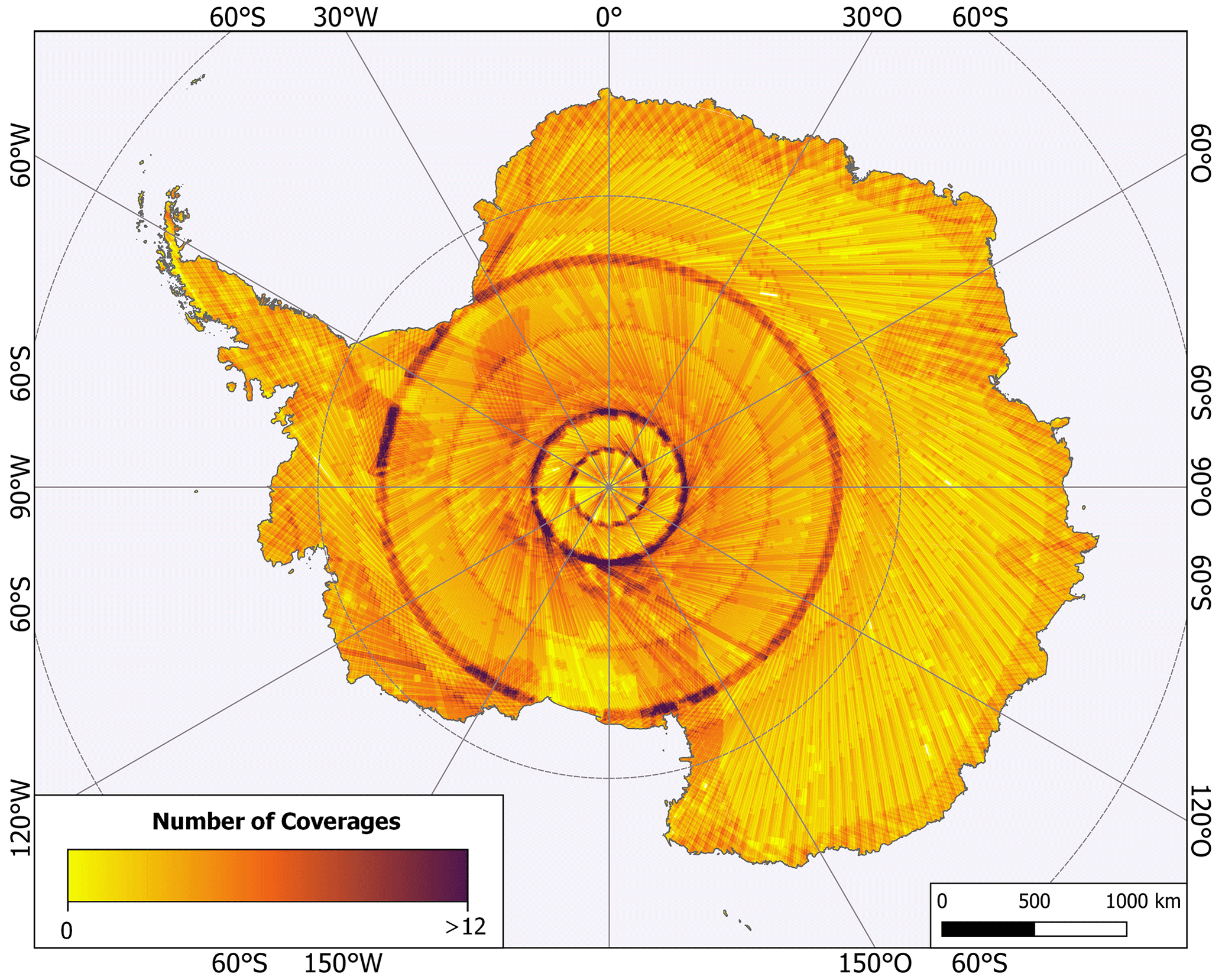
Figure 1 Number of coverages of TanDEM-X DEM data takes.

2.2 ICESat

In 2003 the National Aeronautics and Space Administration (NASA) launched ICESat with the Geoscience Laser Altimeter System (GLAS) on board. GLAS is a laser altimeter designed to measure ice sheet topography with a footprint of about 70 m in diameter spaced at about 172 m along track while not penetrating into the snowpack (Brenner et al., 2007). It observed the ice sheets from 2003 to 2009. The specific data set used for supporting the TanDEM-X mission is the GLAS/ICESat L2 Global Land Surface Altimetry Data, Version 31, GLA14 (Zwally et al., 2012).

To ensure a good height accuracy and to reduce slope-induced elevation errors of ICESat points, we used the classification information provided for each measurement point (Schutz et al., 2005) to select the most reliable points (Hueso Gonzalez et al., 2010). According to a previous accuracy study, the standard deviation for these selected ground control points (GCPs) should be below 2 m under optimal conditions (ICESat points on flat bare land) (Huber et al., 2009), and another study for flat ice areas reports a standard deviation even below 1 m (Brenner et al., 2007). A gross error detection was necessary, because of reflections on clouds, to exclude points with unrealistic heights of more than 100 m difference to TanDEM-X DEM. The estimated Gaussian elevations of ICESat were used as heights and for comparison, and all elevation values of the TanDEM-X DEM within a single ICESat footprint were averaged according to a laser-specific weighting function (Harding and Carabajal, 2005). The quality of the ICESat points is estimated by the number of ICESat peaks and the ICESat signal width (Gruber et al., 2012) in order to obtain ground control points on mainly bare and flat terrain and to avoid points on slopes, local relief, or over noisy areas. For block adjustment, in general only the best 10 ICESat points per 50 km long DEM scenes were used, and a much higher number was used as validation ground control points for the final DEM heights. For reliable validation points, the standard deviation of the TanDEM-X DEM within the footprint must additionally be below 1 m.

For the absolute height accuracy evaluation, a good distribution of points over the whole continent is important. This was realized via a fixed number of points per geocell. The TanDEM-X product is partitioned into geocells whose size is latitude dependent ($\mathrm{1}{}^{\circ }\times \mathrm{2}{}^{\circ }$ between 60 and 80^∘ S and $\mathrm{1}{}^{\circ }\times \mathrm{4}{}^{\circ }$ between 80 and 90^∘ S). In total 2349 geocells were evaluated between latitudes of 60 and 87^∘ S. Note that the geocell rows S88, S89, and S90 do not contain any ICESat points because the polar cap could not be covered due to the ICESat orbit geometry. For each geocell only the 1000 most reliable points in terms of the lowest TanDEM-X height standard deviations within the ICESat footprint were selected for validation. This reduces the original 56 463 474 ICESat points over Antarctica to 2 314 167 and then to 2 150 776 after final selection with the 3σ rule and masking out the frozen ocean for consistent validation of the land mass topography. The height differences were clipped and assigned by means of the land cover map of Hui et al. (2017a).

2.3 Blue ice maps

Blue ice areas (BIAs) are unique to Antarctica and consist of old and compressed ice, extending mainly downwind from protruding rocks (e.g., Orheim and Lucchitta, 1990; Bintanja, 1999). They are distributed across the continent, mostly lateral of inland mountain ranges and nunataks, and in coastal regions with a strong katabatic wind influence. Estimates of BIAs are around 1 % of the Antarctic land surface (e.g., Giovinetto, 1964; Winther et al., 2001; Hui et al., 2017a). Due to the reduced presence of air bubbles compared to glacier ice, blue ice absorbs radiation in the red spectrum and reflects the deeper-penetrating blue, causing the ice to appear bluish. Significant features include a flat and hard surface which is smooth but often rippled because of wind sublimation. The highly densified ice of BIAs cannot be penetrated by the X-band SAR wavelength (Rott et al., 2017; Zhao and Floricioiu, 2017). Blue ice areas therefore are not penetrated by InSAR or laser measurements and are well suited to validate the absolute height accuracy of the TanDEM-X DEM in Antarctica.

An Antarctic land cover database (AntarcticaLC2000) using Landsat-7 Enhanced Thematic Mapper Plus (ETM+) imagery from 1999–2003 and MODIS (Moderate Resolution Imaging Spectrometer) data from 2003–2004 has been produced by Hui et al. (2017a). This data set consists of three classes: snow/firn (97.8 % of the area), ice-free rocks (0.537 %), and blue ice (1.656 %), classified with an overall accuracy of 92.3 % (available at: https://zenodo.org/record/826032#.Wo1zSk2pWUk, last access: 13 June 2020).

For an evaluation of the AntarcticaLC2000 data, a more detailed blue ice classification from the Australian Antarctic Data Centre (AADC) was used (Bender and Smith, 2013). In this data set, which is limited to the Prince Charles Mountains in the Lambert Basin (southern Amery Ice Shelf), areas of blue ice regarded as potential aircraft landing sites were digitized from the Landsat Image Mosaic of Antarctica (LIMA) (USGS, 2008).

In addition, for a test area within this region we performed our own object-based classification based on the Landsat-8 Operational Land Imager (OLI) with a similar acquisition time as the TanDEM-X data (December 2013). In the classification process, we made use of the spectral information, including snow and glacier indices (Normalized Difference Glacier Index, NDGI; Normalized Difference Snow Index, NDSI), as well as texture information (gray-level co-occurrence matrix, GLCM).

2.4 IceBridge measurements

Operation IceBridge is an airborne scanning laser altimeter which bridged the data gap between the ICESat and ICESat-2 missions (Koenig et al., 2010). Since 2009, IceBridge has annually surveyed both the Greenland and Antarctic ice sheets, as well as sea ice and Arctic glaciers. Typically flown at altitudes of 500 m, the ATM illuminates a swath width of approximately 140 m, with a footprint size of 1 to 3 m and along-track separation of 2 m by measuring surface elevation with an accuracy of 10 cm or better (Krabill et al., 2002). In this study we used IceBridge ATM L2 elevation data (Studinger, 2014) to characterize the edited TanDEM-X DEM, although TanDEM-X SAR measurements and the airborne laser altimeter measurements of IceBridge differ over the snow pack in the reflection on the surface and subsurface. Furthermore, the IceBridge program's focus is active glacier areas (Koenig et al., 2010) which lead to temporal changes. Therefore, regarding our validation purpose, we carefully examined the IceBridge data set and selected IceBridge data from the same period and from the most stable regions like the South Pole and the Recovery Glacier, both acquired in October 2014.

2.5 Reference DEMs

For further model-to-model comparisons we used two actual DEM data sets both covering similar time frames as TanDEM-X: the CryoSat-2's radar altimeter DEM from Slater et al. (2018) and REMA (Howat et al., 2019). The CryoSat-2 DEM is composed of measurements between 2010 and 2016 and is posted at a resolution of 1 km. For our comparison, the TanDEM-X DEM was resampled to 1 km Antarctic Polar Stereographic grid spacing. The REMA mosaic is constructed from stereoscopic satellite imagery collected by DigitalGlobe's WorldView satellite constellation acquired mostly between 2015 and 2016 and is distributed in Antarctic Polar Stereographic projection in 8 m. For our purposes, we used the resampled version with 1 km spacing. The vertical reference for all used DEMs is the WGS 84 ellipsoid.

3 DEM generation method

Two processors were involved in the generation of the TanDEM-X DEM product (Wessel, 2018). At first, the Integrated TanDEM-X Processor (ITP) (Fritz et al., 2011; Rossi et al., 2012; Lachaise et al., 2018) interferometrically processed raw data to pre-calibrated, geocoded single-scene DEMs, the so-called RawDEMs. The Mosaicking and Calibration Processor (MCP) performed the final height calibration by a block adjustment (Gruber et al., 2012) and a mosaicking of the corrected single RawDEMs to the final TanDEM-X DEM product (Gruber et al., 2016). The generation of the DEM for Antarctica necessitated a special calibration procedure that we present for the first time in detail in the following sections.

3.1 Antarctica DEM block adjustment

The TanDEM-X block adjustment, also called DEM calibration, is conducted by a weighted least-squares adjustment employing ICESat points, as well as image tie points (TPs). Thanks to the excellent calibration of the TanDEM-X system, only small offsets and tilts for a single data take remain. They are in the range of a few meters, typically $<\pm \mathrm{2}$ m, and are subject to the block adjustment. ICESat points are used as ground control points (GCPs) to adjust the TanDEM-X DEM to the absolute height reference. Tie points are located within a 3 km range overlap between two adjacent acquisitions and are used to derive height differences. For a tie point the height of an area of approximately 1 km × 1 km is evaluated, and the median height is chosen for comparison (Huber et al., 2010).

However, SAR signals penetrate into the ice sheet. The penetration depth depends on the wavelength of the radar and the snow and ice properties (Fischer et al., 2020). Consequently, the SAR measurements are biased relative to the laser-altimeter-derived ICESat elevations, in general lower by several meters (see Fig. 2). Therefore, ICESat points have to be applied in a different way to avoid an artificial rise or even deformation of the resulting DEM upwards to the ground control points. For Greenland, the calibration of the RawDEMs was performed solely with ICESat points measured in the outer coastal rock regions (Wessel et al., 2016), and in the inner ice sheet tie points link the data takes to each other. In contrast, Antarctica's coast is mostly covered by ice, and therefore, the ICESat elevations do not represent the same elevation because of the radar data's penetration bias. For Antarctica, we developed a new innovative approach relying on areas with homogeneous backscattering characteristics and thus a primarily homogeneous penetration bias (HPB; see Fig. 2). Figure 3 describes the workflow for this new DEM adjustment of InSAR data takes over glaciated terrain.

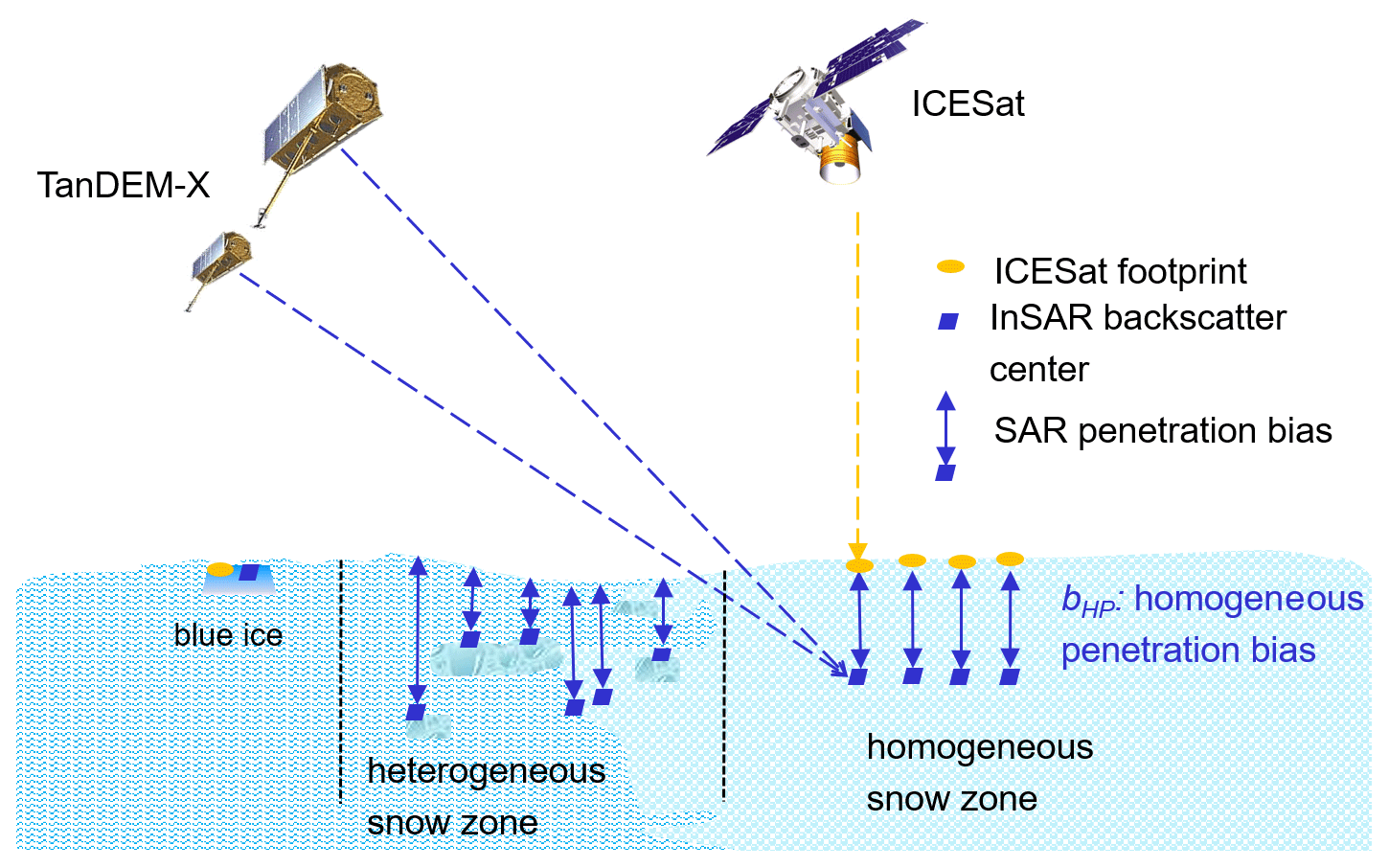
Figure 2 Schematic characterization of the snow-zone-dependent surface penetration of X-band SAR into the ice sheet. b_HP denotes a homogeneous penetration bias for homogeneous snow zones.

Figure 3 Workflow for DEM adjustment of TanDEM-X DEM data takes in Antarctica.

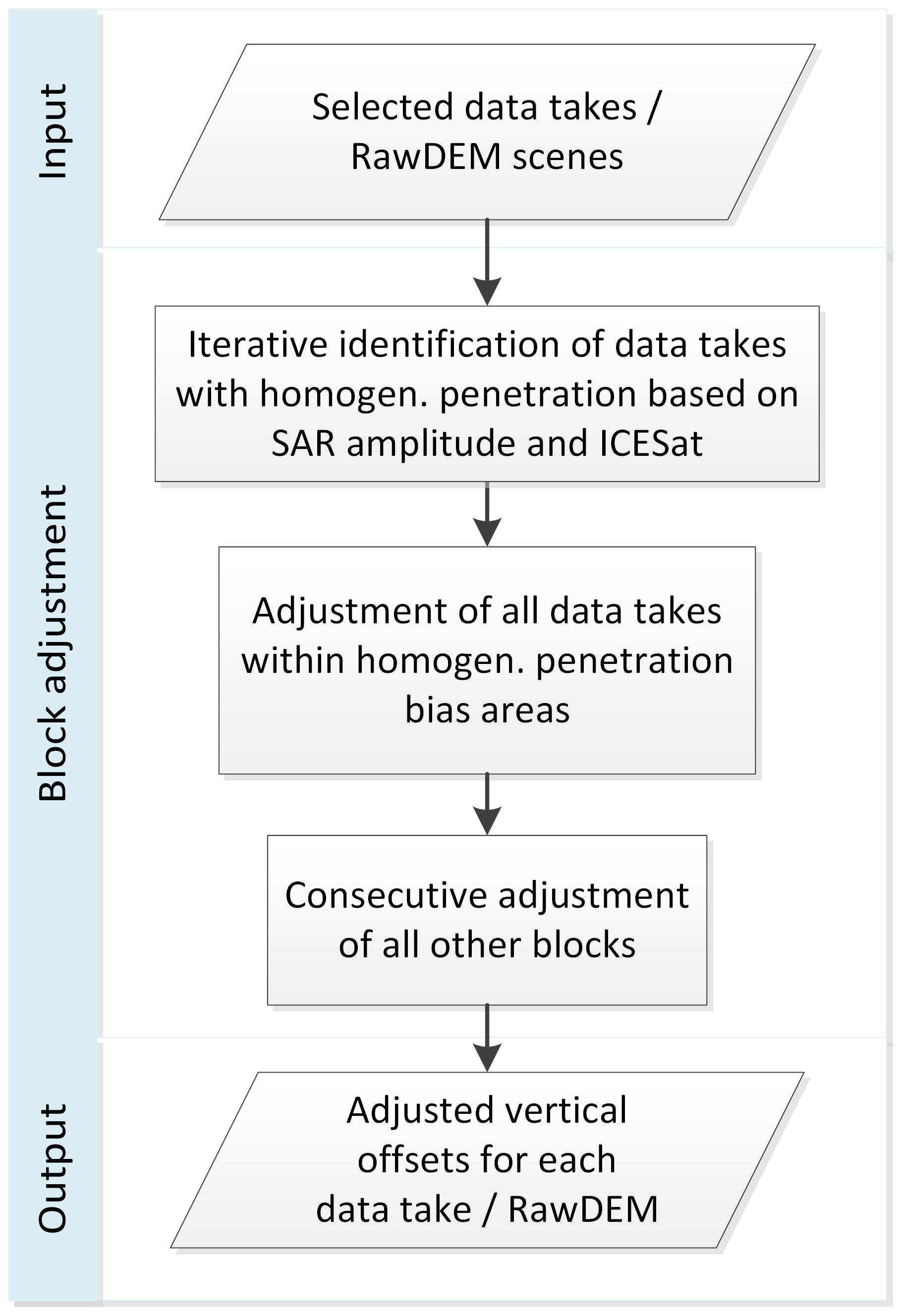
In a first step, the HPB areas must be identified in the inner Antarctic continent with the help of the RADARSAT-1 amplitude mosaic (Jezek, 2002). TanDEM-X data takes over a homogeneous amplitude area located in the dry snow zone were grouped into a so-called adjustment block, i.e., into a consolidation of several data takes over one region. Then, the data takes of this potential homogeneous penetration block L were adjusted by a nominal least-squares adjustment towards the GCPs with the standard observation equation for TanDEM-X heights at GCPs (Gruber et al., 2012) which is aiming at zero height differences given by the equation

$$\begin{array}{}\text{(1)}& \left[H_{i,J}+\widehat{x_J}\right]-H_{i,\mathrm{GCP}}+{\widehat{v}}_i=\mathrm{0},\end{array}$$

where H_i,J is the observed height H_i of data take J, $\widehat{x_J}$ is the adjusted unknown correction parameter for data take J, and ${\widehat{v}}_i$ are the summarized residuals. For Antarctica only offsets a were determined ($\widehat{x}=\widehat{a}$). After this, the mean height difference between TanDEM-X and ICESat elevations was calculated for all data takes of the whole potential homogeneous penetration block. The standard deviation of the height differences (SD_dH) is low for these blocks. This can serve as a measure for a homogeneous InSAR penetration. The extent of the input scenes was iteratively modified yielding standard deviations below 1 m. Finally, we identified 11 homogeneous penetration bias blocks (Fig. 4 in red). For the HPB the mean penetration bias and standard deviations vary from −1.68 to −5.66 m and 0.92 to 1.20 m, respectively. They are located in the interior of Antarctica and are well distributed over the continent to serve as ground control for the adjacent blocks.

In a nominal least-squares adjustment the estimated offsets would be applied, and the DEM data takes would be lifted towards the ICESat GCPs. In order to avoid uplifting effects, for each HPB block L the mean penetration bias b_HP,L based on the difference between TanDEM-X and ICESat elevations,

$$\begin{array}{}\text{(2)}& b_{\mathrm{HP},L}=\mathrm{1}/n\sum _{i=\mathrm{0}}^n{H}_{i,J}-H_i^{\mathrm{GCP}},\end{array}$$

is calculated as a constant bias for the entire block. The application of b_HP,L to the individual data takes sets the height level of the adjusted heights back to a mean InSAR height below the surface:

$$\begin{array}{}\text{(3)}& {\widehat{H}}_{i,J}^{b_{\mathrm{HP},L}}=\left[H_{i,J}+\widehat{x}\right]+b_{\mathrm{HP},L}.\end{array}$$

Note that b_HP,L is negative.

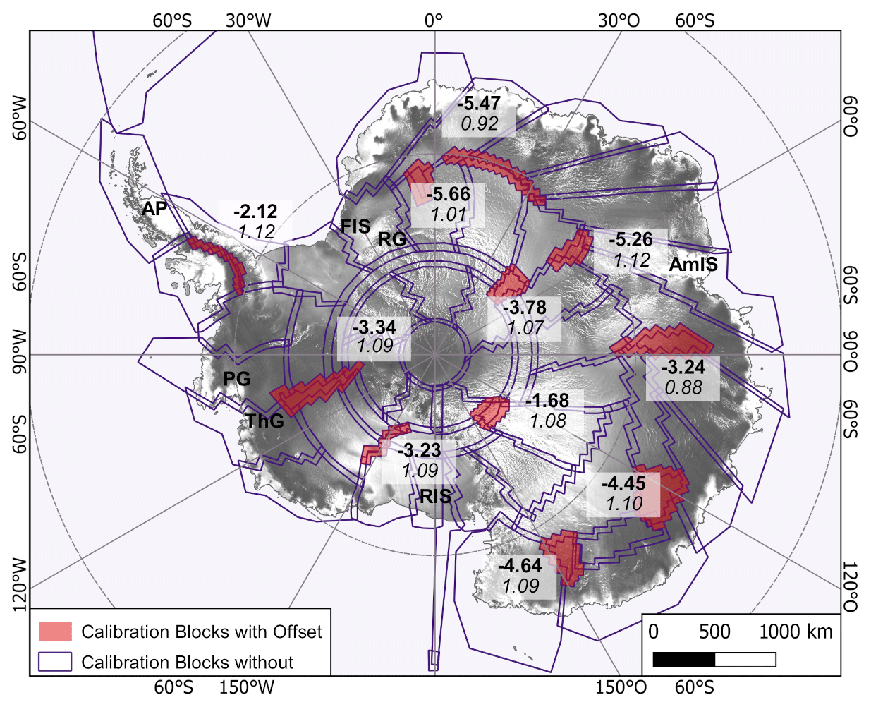
Figure 4 DEM Calibration blocks for Antarctica. The 11 red blocks were calibrated first towards ICESat, and then the mean SAR penetration bias was subtracted. Bold numbers: mean penetration bias per homogeneous penetration block. Italics: standard deviation of TanDEM-X to ICESat elevations. The red blocks were used as ground control areas for the remaining blocks. In black are locations of interest: AP: Antarctic Peninsula; AmIS: Amery Ice Shelf; FIS: Filchner Ice Shelf; PG: Pine Island Glacier; RG: Recovery Glacier; RIS: Ross Ice Shelf; ThG: Thwaites Glacier.

Starting from these ground control blocks, all other DEM acquisitions were adjusted relying solely on tie points and on already adjusted heights from neighboring blocks that were used as ground control point heights using Eq. (1). Further on, the observation equation for tie points also sets the height difference of two heights $H_J^{\mathrm{TP}}$ of data take J and $H_K^{\mathrm{TP}}$ of data take K to zero:

$$\begin{array}{}\text{(4)}& \left[H_{i,J}^{\mathrm{TP}}+{\widehat{x}}_J\right]-\left[H_{i,K}^{\mathrm{TP}}+{\widehat{x}}_K\right]+{\widehat{v}}_i=\mathrm{0}.\end{array}$$

The DEM calibration process of the 50 blocks without external GCPs (Fig. 4 in blue) started in East Antarctica and proceeded in two directions, clock-wise and counter-clockwise, re-unified in West Antarctica. In summary, the DEM calibration strategy for Antarctica can be subdivided into two parts:

• First, all homogeneous penetration bias blocks are adjusted by maintaining the mean penetration with respect to ICESat.

• Second, all other DEM acquisitions are adjusted relying solely on tie points and on already adjusted heights from other blocks.

3.2 DEM mosaicking concept

The aim of DEM mosaicking is the fusion of individual DEM scenes into a complete and homogeneous elevation model. Basically, all acquired data were considered in the TanDEM-X DEM product generation process to reduce the random height error (HE). The individual pixels were mosaicked according to an HE-weighted average:

$$\begin{array}{}\text{(5)}& h_i={\displaystyle \frac{\sum _{k=\mathrm{1}}^K\frac{\mathrm{1}}{{\mathit{\sigma }}_{\mathrm{HE},k}^{\mathrm{2}}}{h}_k}{\sum _{k=\mathrm{1}}^K\frac{\mathrm{1}}{{\mathit{\sigma }}_{\mathrm{HE},k}^{\mathrm{2}}}}}.\end{array}$$

For each input elevation h_k, the corresponding weight is derived from its height error, a standard deviation estimate σ_HE,k obtained from the interferometric coherence. The estimated calibration correction parameters for each acquisition were applied in advance to each single input DEM scene. In the case of larger height discrepancies induced, for example, by phase unwrapping errors, the TanDEM-X mosaicking approach performs a grouping of all input height measurements into several height intervals (Gruber et al., 2016). This allows for the identification of the most reliable height interval based on InSAR-specific parameters.

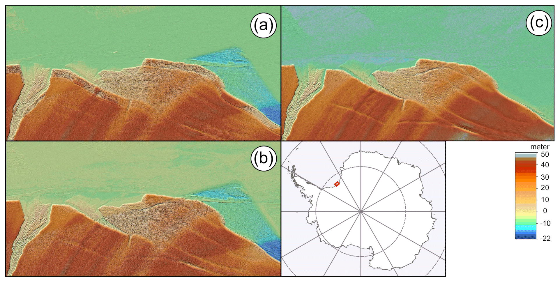
Figure 5 DEM mosaicking iterations at Filchner ice shelf. (a) First mosaicking with all acquisitions from mid-2013 and mid-2014, (b) second mosaicking with 2014 acquisitions only, and (c) third mosaicking with 2014 ascending acquisitions only.

Nevertheless, some continuous changes near the coast could be observed even though the acquisition time span was relatively short. Surface melting, tidal effects on floating ice, and glacier or ice shelf advances that caused height disparities between the input data were some of the main challenges for the mosaicking. Thus, the quality assessment of the mosaicking results had to be conducted with regard to these conflicting measurements, with the consequence that contradictory measurements were taken out. In a first step of this iterative quality control process, all acquisitions were mosaicked in the same way as for the standard TanDEM-X DEM generation. In a follow-on step, conflicting DEM scenes were identified and removed for a second mosaicking run. This identification and mosaicking step had to be repeated one to three times. Figure 5 illustrates such a first all-in mosaicking result at the Filchner ice shelf and its iterative improvement by omitting some contradicting scenes. The initial mosaicking resulted in multiple mappings of the ice shelf front and the crevasses caused by the ice drift at different acquisition times (Fig. 5a). In the first improvement step the acquisitions of mid-2013 were omitted to reduce the effects of ice drifts between 2013 and 2014 (Fig. 5b). In a second iteration, all scenes from the crossing orbits (in this case with a descending orbit look direction from mid-2014) were additionally taken out, eliminating edge effects and providing a smoother DEM (Fig. 5c).

4 DEM editing

The global TanDEM-X DEM is an unedited DEM created from SAR interferometry. This implies, among other effects, that open water surfaces show noisy relief due to low coherence and backscatter. In order to enhance the usability for further applications such as orthorectification, ice velocity, or mass balance estimation, a filling and editing of the TanDEM-X DEM was conducted with special focus on the coasts. These improvements are made under the TanDEM-X PolarDEM framework for the provision of derivatives of the global TanDEM-X DEM for polar regions. The derivatives currently include a filled and edited version of the TanDEM-X DEM for Antarctica as described in this section. It will be supplemented in the future by the TanDEM-X PolarDEM for the Arctic, especially over Greenland, with single year coverages and penetration-bias-corrected DEMs.

4.1 DEM gap filling

Although the acquisition strategy planned at least two complete acquisitions, several factors contributed towards insufficient RawDEM quality or missing acquisitions (e.g., inappropriate height of ambiguity for dual-baseline phase unwrapping and loss of data during downlink; a more detailed list is given in Rizzoli et al., 2017). For Antarctica, this in turn yielded 16 small data gaps within the TanDEM-X DEM with a total size of 13 200 km² affecting 52 geocells as displayed in Fig. 6. Additional acquisitions were subsequently scheduled for these gaps as DEM geocells containing gaps were identified during the quality assurance process within the ground segment. For Antarctica these acquisitions were performed from mid-2016 to mid-2017.

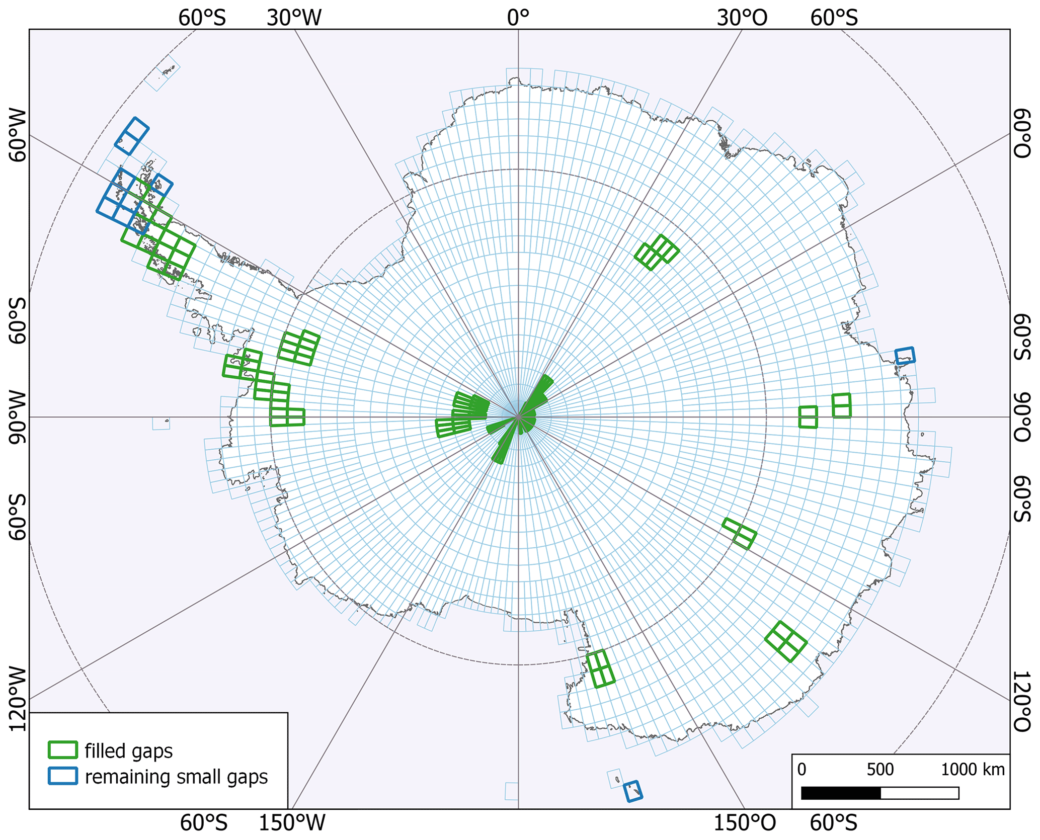
Figure 6 TanDEM-X DEM geocells after DEM gap filling with new acquisitions: geocells with gaps that could be filled are in green. Geocells with remaining smaller gaps after DEM gap filling are in blue.

A major improvement in coverage could be achieved by incorporating 20 new acquisitions for Antarctica (see geocells with improved coverage in Fig. 6). All new DEM scenes were calibrated onto the existing DEM scenes, and all related geocells were re-mosaicked including all previous and new DEM scenes. The resulting filled TanDEM-X DEM built the basis for later editing. Finally, a coverage completeness of 99.991 % of the total Antarctic land mass could be achieved. Note that remaining smaller gaps with a total size of 1200 km² are located over islands and the Antarctic Peninsula, while the rest of mainland Antarctica is completely covered by TanDEM-X elevation data.

4.2 Semi-automatic coastline delineation

In order to demarcate the Southern Ocean, an outline of Antarctica was derived based on the 0.4 arcsec (approximately 12 m) TanDEM-X elevation (DEM) and amplitude (AMP) layers. This outline represents the separating line between open sea and ice shelf or land areas rather than the actual divide between land and water. For the sake of convenience the term “land” comprises the ice shelf and land areas in the following. The TanDEM-X-derived outline therefore distinguishes between open sea and land and is called “TanDEM-X coastline”. During the DEM editing, homogeneous geoid undulations were assigned to the open sea areas, while identified land areas were further edited as described in Sect. 4.3.

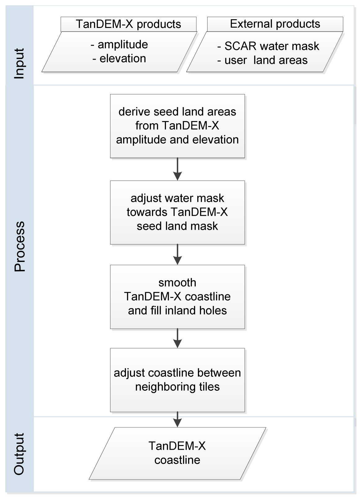
Figure 7 illustrates the workflow for the tile-based coastline delineation. The input data includes the 0.4 arcsec TanDEM-X elevation (DEM) and amplitude (AMP) layers of the TanDEM-X DEM product (Wessel, 2018). Additionally, the coastline from the Scientific Committee on Antarctic Research (SCAR) provided via the Antarctic Digital Database (ADD) is utilized as a proxy for the coastline (Scientific Committee on Antarctic Research, 2019). For integration into the workflow the SCAR coastline was rasterized in 0.4 arcsec. In the following, this rasterized proxy is referred to as SCAR water mask. It is adapted where necessary by adding user-defined sea and ice shelf or land areas, respectively. Note that shelf ice or land areas will only survive where corresponding seeds exist within the water mask. Moreover, a set of variable configuration parameters can be set for each tile, e.g., AMP and DEM thresholds. Therefore, the approach is referred to as semi-automatic since tile-specific conditions may require individual adjustments.

Figure 7 Workflow for (semi-)automatic TanDEM-X coastline delineation.

In a first processing step, a seed land mask is derived from the AMP (Fig. 8a) and DEM (Fig. 8b) layer using default or user-specific thresholds. For the amplitude layer land areas are assumed to have values above a default threshold of, for example, 100 in digital numbers. The threshold for the elevation layer is based on the mean geoid height plus a default threshold of, for example, 10 m; i.e., land areas are assumed to be higher than the mean sea level plus a defined margin. For the seed land mask both thresholds (AMP and DEM) have to be fulfilled (Fig. 8c). In the second processing step, the rasterized SCAR coastline is taken as the starting line and is gradually adjusted to the extent of the TanDEM-X seed land mask using dilation and erosion operations (Fig. 8c). In other words, the SCAR coastline is extended towards the open sea where TanDEM-X indicates land and extended towards land where TanDEM-X indicates water. This approach also eliminates false positive errors in the TanDEM-X seed land mask (e.g., presumed islands which are actually icebergs), as well as false negative errors (e.g., presumed water areas within land which are indicated due to low amplitude values on land ice). Afterwards, filter operations were applied to smooth the resulting coastline and fill remaining inland holes in the land mask. Neighboring tiles may show misalignment in their coastlines due to varying configuration parameters and tile-based processing. Therefore, an automatic correction is applied to match detected coastlines of adjacent tiles. The resulting outline (Fig. 8d) is utilized during the following editing process in order to replace open water areas by geoid undulations. The length of the derived TanDEM-X coastline of Antarctica is 62 971 km. It should be noted that the generated outline reflects the conditions as observed by the TanDEM-X mission mainly in the years 2013 and 2014.

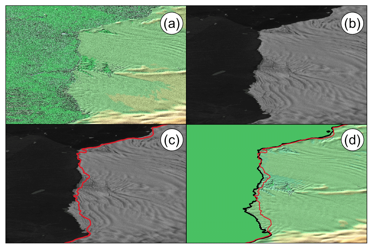
Figure 8 TanDEM-X semi-automatic coastline delineation – example of Mackenzie Bay, Amery Ice Shelf. (a, b) Input: DEM and amplitude of TanDEM-X DEM, (c) SCAR coastline superimposed in red, and (d) TanDEM-X coastline derived from DEM and amplitude in black and SCAR in red, superimposed on tailored and geoid-filled DEM.

4.3 Semi-automatic DEM editing

All 0.4 arcsec TanDEM-X DEM tiles of Antarctica run through the general editing workflow developed for TanDEM-X DEMs which is described in Huber et al. (2021). Focus is on edge-preserving smoothing, as well as the void and outlier interpolation, especially for areas with strong relief located mainly in outer Antarctica.

• Edge-preserving smoothing. An edge-preserving smoothing was applied to the whole dataset. On the one hand, this provides a smoother dataset by reducing local noise. On the other hand, linear structures like ridges and peaks are preserved as the smoothing does not weight pixels on different sides of these linear DEM features.

• Outlier and void interpolation. Due to the processing characteristics of radar data, single outlier pixels may be present in the elevation data. Although multiple radar acquisitions are fused during the TanDEM-X DEM generation (Gruber et al., 2016), an outlier detection and local interpolation is implemented. The outlier pixels are defined based on local statistics and interpolated with the same approach as for the smoothing. However, the center pixel, which is supposed to be unreliable, receives zero weight and is therefore neglected.

  Also, void pixels caused by low coherence may be present. They are interpolated from surrounding elevations by a variance-weighted averaging by considering the variance values provided within the height error map, as well as a variogram model describing the degree of spatial dependence of the neighboring pixels.

• Integration of geoid undulations for the ocean mask. To provide heights for the ocean, the geoid undulation N is chosen. The geoid undulation represents the deviation of the geoidal height h_MSL from the ellipsoidal height h_ell:

  $$\begin{array}{}\text{(6)}& N=h_{\mathrm{ell}}-h_{\mathrm{MSL}}.\end{array}$$

  This ensures that when ellipsoid heights are converted to mean sea level, the ocean height values in geoid heights correspond to zero mean sea level. The geoid undulations are extracted from the commonly used Earth Gravitational Model 2008 (EGM2008 Development Team, 2012). In order to support a smooth transition between geoid and TanDEM-X heights, a buffer zone of approximately 200 m is defined starting from the coastline towards the open sea. Within this buffer zone the geoid undulations and TanDEM-X heights are combined by distance-weighted averaging.

• Reduction and resampling to 90 m. The TanDEM-X PolarDEM of Antarctica was first reduced to 1 arcsec pixel spacing by an unweighted mean of the underlying 0.4 arcsec pixels. For more convenient data handling the DEM in geographic coordinates subdivided into 2621 tiles south of 60^∘ S was transformed into the more suitable Cartesian coordinates in the Antarctic Polar Stereographic projection (EPSG:3031) with a pixel spacing of 90 m (Fig. 9).

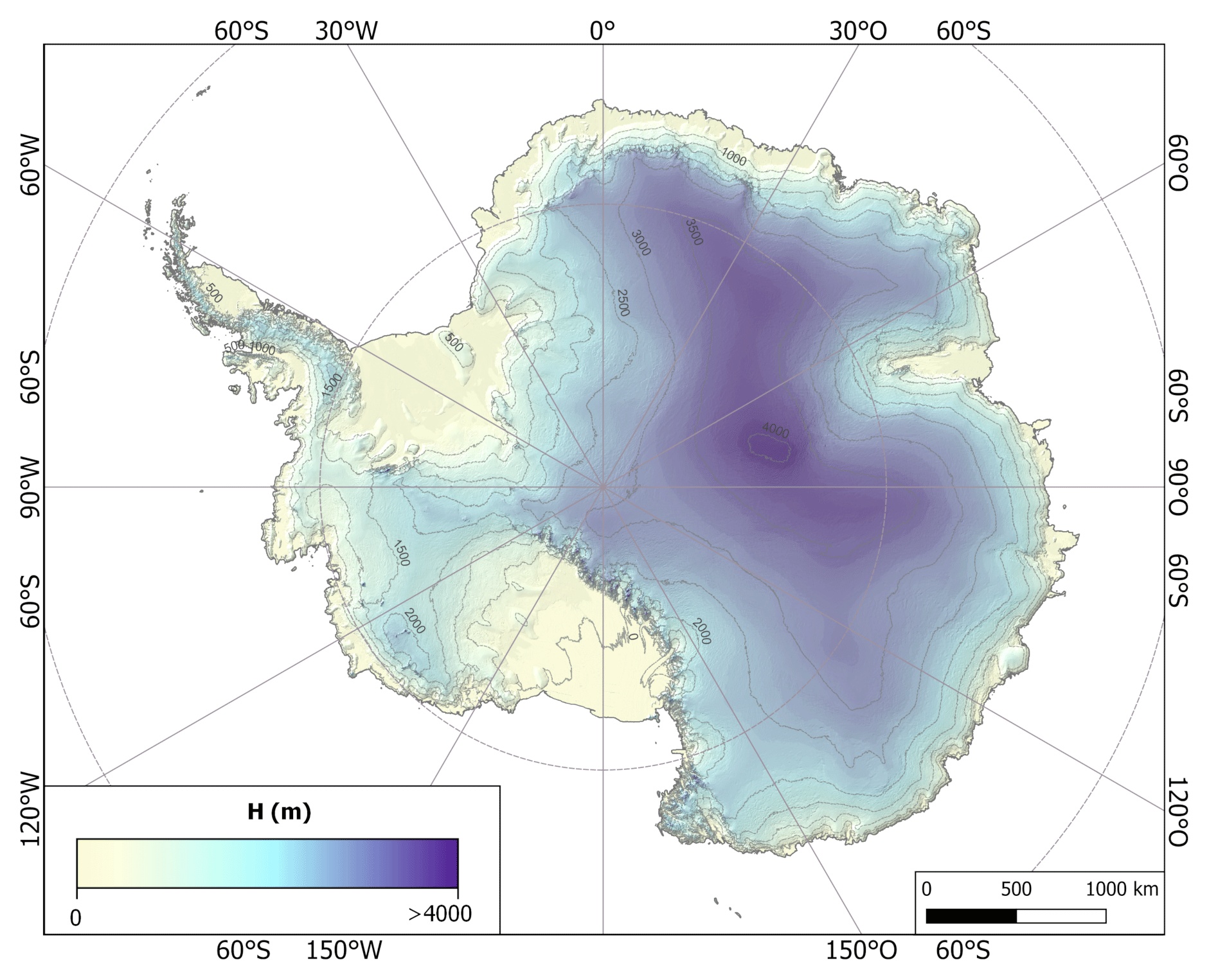
Figure 9 Gap-filled and edited TanDEM-X PolarDEM 90 m of Antarctica in color-coded elevations.

5 Results and discussion

The evaluation and error characterization of the vertical accuracy of the TanDEM-X PolarDEM of Antarctica is based on the comparison with ICESat, IceBridge, and other DEM data. The results are detailed in the following.

5.1 Quality characterization with ICESat

The resulting accuracy numbers in comparison with ICESat are given in Table 1. As the height differences are defined as TanDEM-X height minus ICESat height, negative height differences, like the mean of −3.22 m, mean that the InSAR heights are below the laser-based ICESat heights. This can mainly be explained by the SAR signal penetration into ice in the order of a few meters. The deepest penetration bias into the glaciated surface can be found at the highest elevations in the central East Antarctic ice sheet (AIS) (Fig. 10). Here, the temperatures are coldest (Macelloni et al., 2019; Scambos et al., 2018), and the SAR signal penetrates the most in dry, cold firn (Ulaby et al., 1986), whereas the coastal areas show lower penetration which clearly corresponds to the brighter reflecting percolation areas in the amplitude mosaic (Fig. 11). This variation in the SAR penetration over the whole AIS raises the absolute linear error (LE90) to 6.25 m, which is calculated by sorting the absolute differences thresholded by 90 % of the values. A LE90 of 6.25 m is still below the mission requirement of 10 m LE90 for TanDEM-X DEM, though the absolute height accuracy of all geocells worldwide without Antarctica yields an LE90 value of just 3 m (Rizzoli et al., 2017).

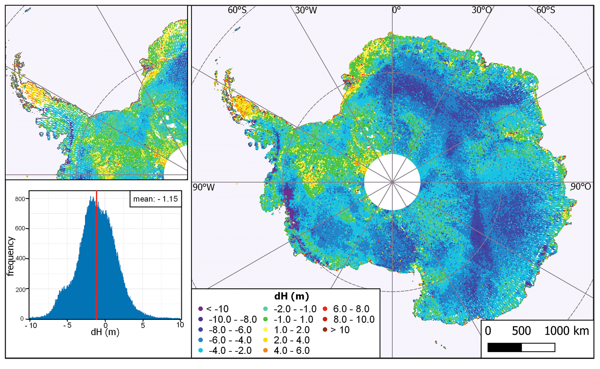
Figure 10 Height differences of TanDEM-X DEM minus ICESat GLA14 elevations over all of Antarctica. Panel on the left: a detailed view on the quadrant of the Antarctic Peninsula with its corresponding histogram of height differences.

Table 1 Accuracy numbers for height differences of TanDEM-X minus ICESat for the whole of Antarctica and individual classes of blue ice areas, snow/firn, and ice-free rocks according to AntarcticaLC2000.

To analyze these variations in the absolute height statistic, the TanDEM-X DEM is subdivided into three different land-cover classes: blue ice areas, snow/firn, and ice-free rocks (Table 1). Looking at the histograms of the height differences (Fig. 12) the most symmetric distribution around zero is given for the blue ice class. Here, we have the lowest absolute median with −0.25 m. In contrast, the class snow and ice shows a slightly uneven distribution with a negative median of −3.38 m due to different penetration biases on different snow facies. Looking at the class ice-free rocks there seems to exist two maxima, one around −1.5 m and one around 2.5 m. However, the differences of the class ice-free rocks should rather be distributed around zero. The points contributing to this class lie mainly in the Transantarctic Mountains and on the Antarctic Peninsula. The ICESat differences in Fig. 10 show positive height differences, especially the northern part of the peninsula, so these points contribute to the peak around 2.5 m in Fig. 12c.

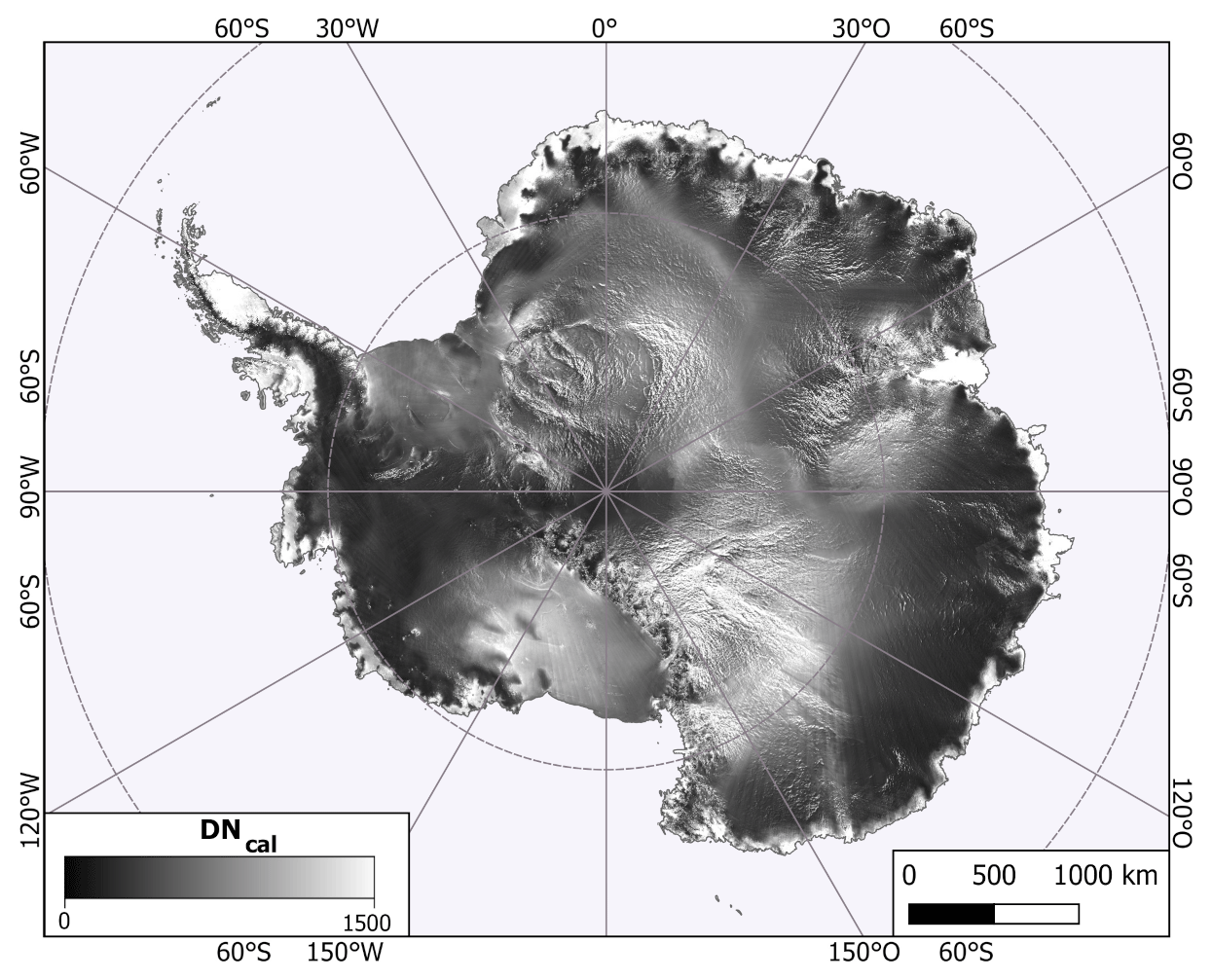
Figure 11 TanDEM-X PolarDEM 90 m amplitude mosaic of Antarctica.

Also in the western AIS, another effect is prominent in a closer analysis of the height differences to ICESat in Fig. 10: in the area around 90^∘ W the height differences increase from negative values to 0 m. Also the differences of the BIA (Fig. 13) increase around 90^∘ W and 80^∘ S in a way that the TanDEM-X elevations are even some meters above ICESat elevations, which is quite unrealistic for a larger area. These differences indicate that the DEM calibration in western Antarctica is erroneous and an increase in the DEM by a few meters has occurred.

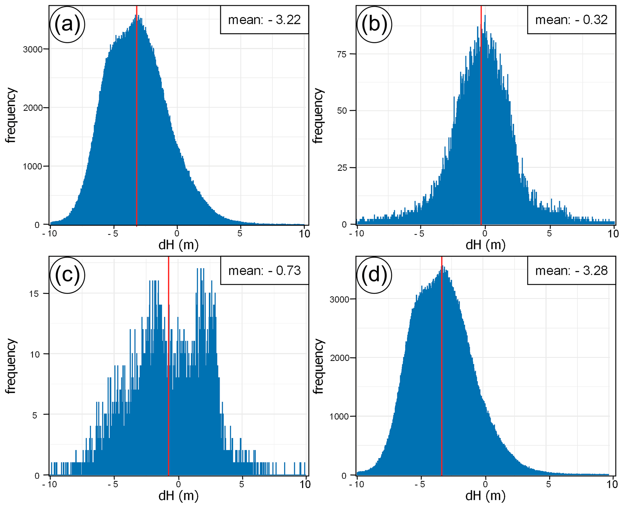
Figure 12 Histograms of height differences of TanDEM-X DEM minus (a) all ICESat elevations, (b) ICESat elevations on blue ice areas, (c) ICESat elevations on ice-free rocks, and (d) ICESat on snow/firn. Assigned according to the land cover map of Hui et al. (2017a).

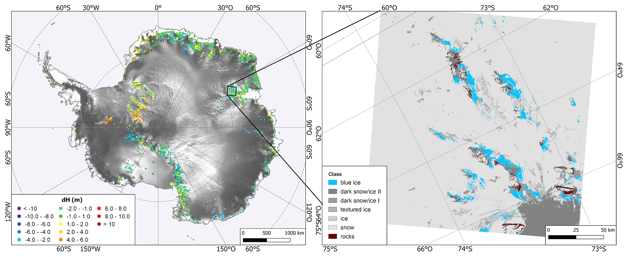
Figure 13 Left panel: distribution of TanDEM-X minus ICESat differences on AntarcticaLC2000 BIAs. Right panel: study area for BIA classification, southern Prince Charles Mountains, Amery Ice Shelf.

Another interesting feature in the differences to ICESat (Fig. 10) can be found in central Antarctica. Here, deeper and shallower InSAR penetrations alternate in a ray structure centered at the pole. It should be noted that the latitudes from −88 to −90^∘ over Antarctica have no ICESat points as the ICESat system did not cover this region. The larger penetration biases are related to darker areas in the amplitude mosaic and lower penetration biases to brighter amplitude areas (Fig. 11). Wind dynamics possibly form together with the underlying ice topography with special characteristics, such as megadunes, snow-glaze areas, and local accumulation highs (Scambos et al., 2012). Glazed surfaces cover the leeward faces where the grain size is increasing, which leads to an increasing backscatter.

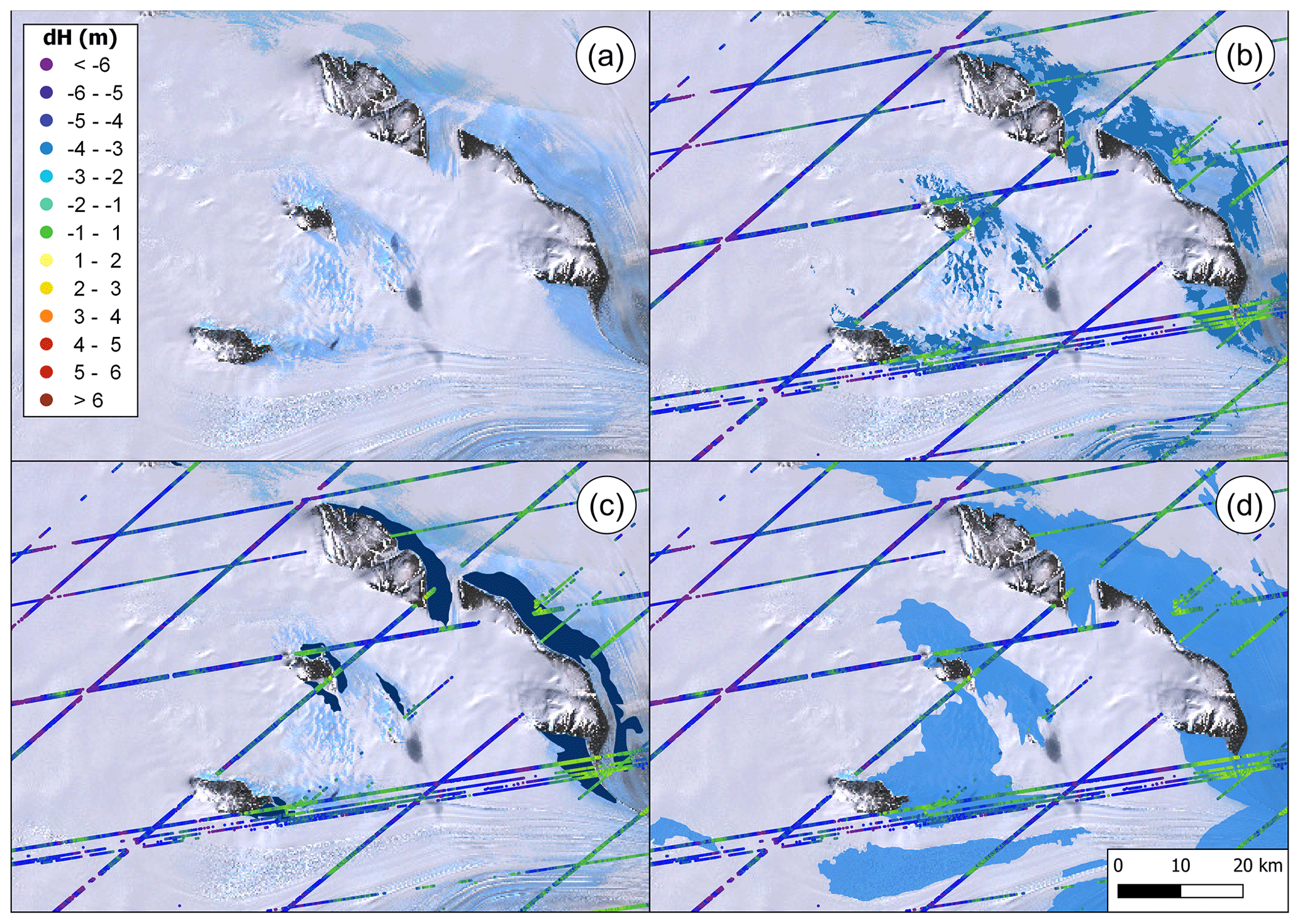
Figure 14 (a) Subset of Landsat image used for classification, (b) proposed BIA classification, (c) AADC BIAs, and (d) AntarcticaLC2000 BIAs. Panels (b–d) are overlaid with the height differences of TanDEM-X minus ICESat.

Generally, these height differences between ICESat and TanDEM-X confirm that the chosen DEM calibration strategy was justified to maintain the different penetration effects and not to raise the DEM towards ICESat elevations to prevent a deforming of the DEM. The assumption could be confirmed that these differences are stable over large areas with homogeneous backscatter (compare to Figs. 10 and 11). Note that the time difference between ICESat and TanDEM-X PolarDEM is the reason for some regional height differences in dynamic areas; e.g., the known decreases at Thwaites and Pine Island glaciers, as well as on the peninsula, are clearly visible in the height differences (Fig. 10).

5.2 Validation with ICESat on blue ice areas (BIAs)

As shown in Sect. 5.1, BIAs are ice areas that the X-band SAR signals do not penetrate. Therefore, a validation of the absolute vertical accuracy of the final TanDEM-X PolarDEM can be achieved through an evaluation with ICESat over BIAs. The results obtained in the previous section rely on a BIA mask from the AntarcticLC2000. For a deeper understanding, we conducted an analysis over a smaller region of the Amery Ice Shelf with a more accurate reference BIA map from the Australian Antarctic Data Centre (AADC) and our own supervised classification optimized for this region. In Fig. 14 all classification results for blue ice for this subset are displayed and are overlaid with TanDEM-X minus ICESat height differences. Over the BIAs, the differences are around zero (green ICESat points) compared to a SAR signal penetration of several meters outside the BIAs. A visual inspection of the blue ice classifications in the southern Prince Charles Mountains test area near Amery Ice Shelf show that the AntarcticaLC2000 classification (Fig. 14d) identified much larger BIAs, whereas the AADC map (Fig. 14c) seems to underestimate these. The purpose of our classification (Fig. 14b) is a more precise delimitation of visible BIAs based on Landsat-8 imagery. It includes additional classes such as highly textured ice or dark snow/ice for a further differentiation.

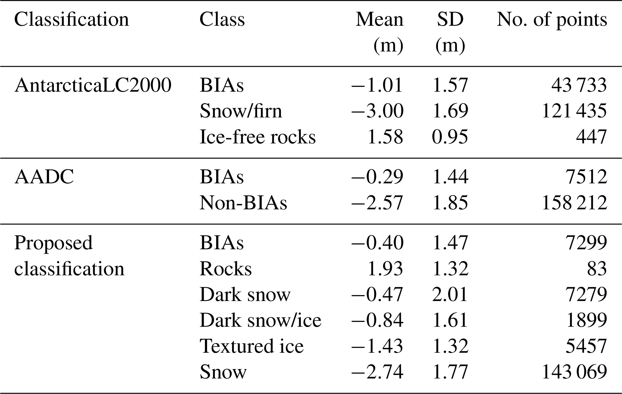
For all three BIA classifications in the test area, we calculated height accuracy measures (Table 2). It could be shown that for all three classifications within this small subset the BIA classes show the lowest mean values. The height accuracy measures in Table 2 confirm the deepest mean penetration for BIAs for AntarcticaLC2000, which is in line with the visual inspection of the data.

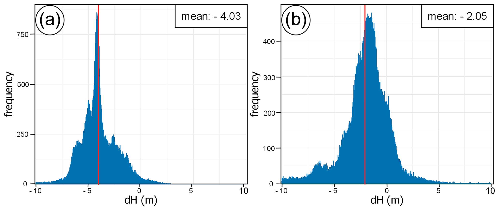
Figure 15 Histograms of TanDEM-X DEM minus IceBridge ATM differences for October 2014 campaigns at the (a) South Pole and (b) Recovery Glacier.

For our proposed classification, the mean difference between TanDEM-X and ICESat is only −0.4 m on BIAs compared to −2.74 m on snow. On dark snowy/icy and textured areas, the mean difference is still more than twice that of BIAs (−0.84 m), with highly textured ice showing the greatest difference within this group (−1.43 m). Areas with a high reflectivity in the short-wave spectrum are generally adjacent to BIAs and show just a small difference between TanDEM-X and ICESat (−0.47 m). The result for the AntarcticaLC2000 data set for all of Antarctica (Table 1) shows that despite the presumed overestimation of BIAs, the height difference between TanDEM-X and ICESat is significantly smaller (−0.32 m) than for snow/firn (−3.28 m) or ice-free rocks (−0.73 m). Though the AntarcticaLC2000 data set performed worse in the local Amery study test site (with a mean of −1.01 m compared to more fine-tuned classifications with mean values of −0.29 and −0.40 m), it is the only one with a complete coverage, and the results for all of Antarctica show a mean of just −0.32 m offset and a mean standard deviation of 2.46 m (Table 1). These findings are in line with first results from the literature (Zhao and Floricioiu, 2017) that find no significant X-band penetration into BIAs. From these results, it can be concluded that BIA is very well suited for the absolute height calibration and validation of InSAR DEMs.

Table 2 Accuracy numbers for height differences of TanDEM-X minus ICESat for different classifications of the southern Prince Charles Mountains (Fig. 13).

5.3 Comparison to IceBridge

Figure 15 shows the distribution of height differences between TanDEM-X DEM and the IceBridge elevation measurements acquired in October 2014 for two test sites which are located around the South Pole (Fig. 15a) and at the Recovery Glacier in the northwest of the AIS (Fig. 15b).

Table 3 Accuracy numbers for height differences of TanDEM-X minus IceBridge for October 2014 campaign.

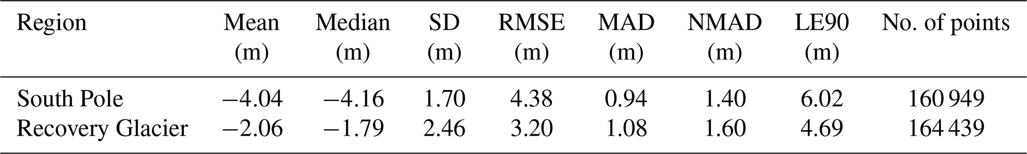
The corresponding statistical metrics are given in Table 3, and in addition, Fig. 16 shows the spatial distribution of the height differences for the two test sites. The differences between TanDEM-X DEM and IceBridge elevation measurements at the South Pole shown in Fig. 15a are distributed around a mean value of −4.04 m with a standard deviation of 1.70 m. The NMAD (normalized median absolute deviation), which represents a robust estimate for the standard deviation for non-normally distributed height differences (Höhle and Höhle, 2009), is quite small with a value of 1.40 m, while the LE90 is 6.02 m (Table 3). In contrast, Fig. 15b shows the height difference histogram at Recovery Glacier with a lower mean value of -2.06 m between TanDEM-X DEM and IceBridge elevation measurements and a higher standard deviation (2.46 m) but with a similar NMAD of 1.60 m. The larger deviation between TanDEM-X and IceBridge elevations at the South Pole is caused by deeper penetration of the SAR signals, which is related to lower backscatter intensity as shown in Fig. 16 (upper left). The higher variance in height differences at Recovery Glacier indicates a higher variability in signal penetration, which is also reflected in the higher variability in backscatter intensity (Fig. 16, upper left) but could also be attributed to subglacial lake drainage (Fricker et al., 2014; Floricioiu et al., 2016). The large number of height differences around zero at Recovery Glacier is due to areas with negligible signal penetration caused by surface scattering, which in turn leads to higher backscatter intensity, as can be seen in Fig. 16.

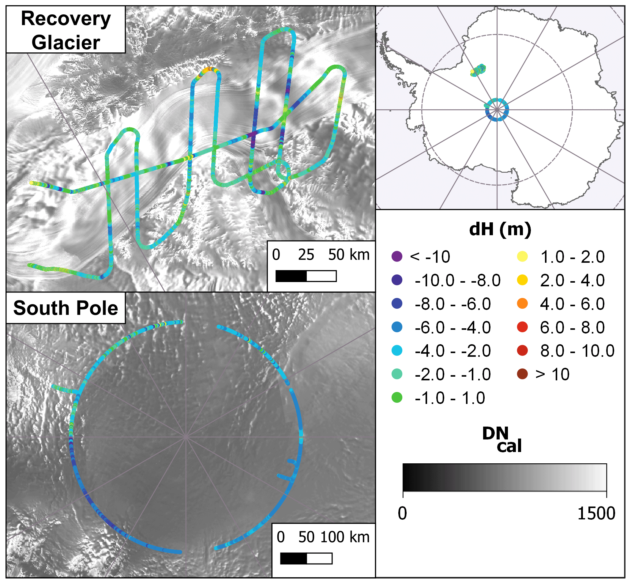
Figure 16 Height differences of TanDEM-X DEM minus IceBridge from October 2014 campaigns over the South Pole and the Recovery Glacier displayed over the amplitude mosaic.

In general, the best agreement between TanDEM-X DEM and IceBridge elevation measurements can be observed over regions with high backscatter intensity associated with low signal penetration. In contrast, the TanDEM-X DEM can deviate from the IceBridge elevation measurements by up to 10 m and more in areas with deep signal penetration, which can be identified by low backscatter intensity.

5.4 Comparison to CryoSat-2 DEM and REMA

The height differences of the TanDEM-X PolarDEM 90 m to the CryoSat-2 DEM of Slater et al. (2018) and the REMA DEM (Howat et al., 2019) were calculated, and the accuracy measures are given in Table 4. For TanDEM-X minus CryoSat-2 we observe a high negative mean value of −11.59 m with high standard deviation (70.58 m) and RMSE (71.53 m) values. These values are in strong contrast to the more robust median (−4.52 m) and NMAD (3.49 m) and suggest a large amount of outliers. These are particularly located in mountainous areas where CryoSat-2 systematically underestimates the elevation. Therefore, strict outlier detection was performed by clipping the height differences above mean ±2 times standard deviation. This improves the measures and results in a mean value of −5.26 m with a standard deviation of 15.21 m.

Figure 17 shows the color-coded height differences, with clipped outlier values marked in white. These areas can be found particularly in mountains where TanDEM-X InSAR and CryoSat-2 altimeter measurements diverge by up to several hundred meters. In contrast, the differences on the ice sheet show a high agreement, apart from the higher SAR signal penetration of TanDEM-X usually between −4 and −10 m in the interior of Antarctica. These penetration patterns correspond to the ones observed by ICESat (Fig. 10), in which the highest penetration-related differences are also in central Antarctica and between 0 and 30^∘ E. A sector in West Antarctica (between 90 and 150^∘ W) also shows higher differences between TanDEM-X and CryoSat-2 of up to −10 m. However, the shape of this higher difference zone seems to be related to the processing windows of CryoSat-2. The interior of the CryoSat-2 DEM was processed by radar altimetry by the low-resolution mode (LRM), a pulse-limited altimetry with a 2.25 km² footprint. The ice sheet margins were processed by the higher-resolution SARIn (SAR Interferometric) mode, in which CryoSat-2 operates as a SAR altimeter. These areas near the coasts generally coincidence well with the TanDEM-X heights. On the one hand, the TanDEM-X DEM elevations in this area are less affected by a penetration bias. On the other hand, it seems that CryoSat-2 has a penetration dependency on the processing method (Slater et al., 2019) because the mode mask boundary between CryoSat-2 LRM and SARIn processing modes is obviously visible (Fig. 17).

Table 4 Accuracy numbers for height differences of TanDEM-X minus CryoSat-2 (CS2) DEM (Slater et al., 2018) and REMA (Howat et al., 2019).

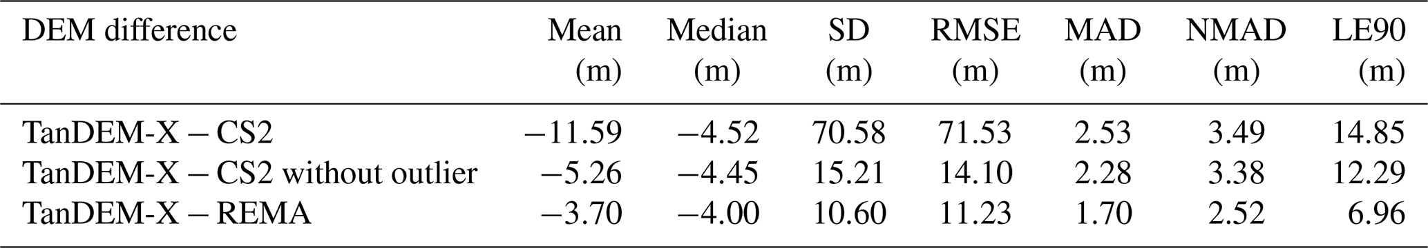
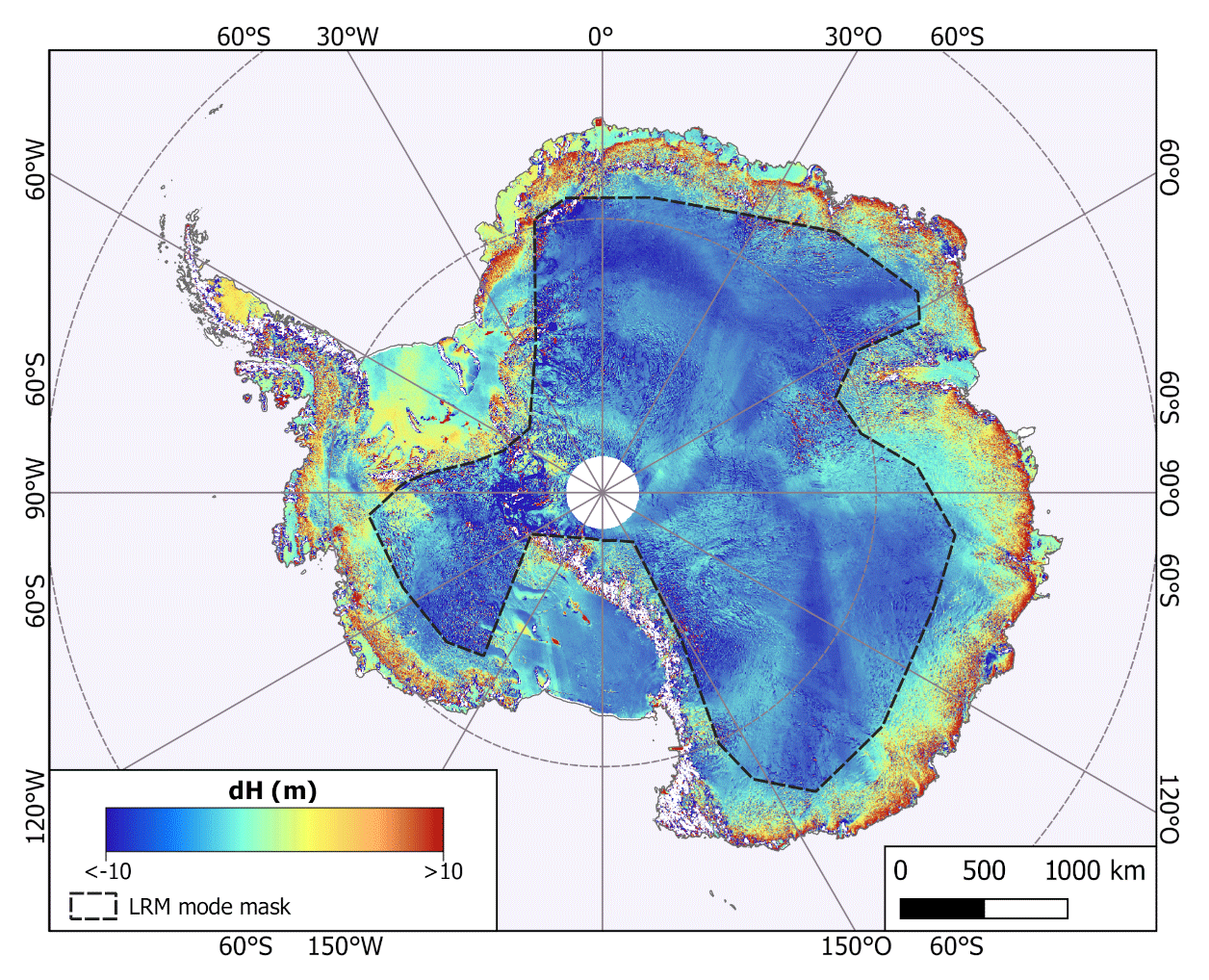
Figure 17 Height difference of TanDEM-X DEM minus CryoSat-2 DEM (rocks: mean $\pm \mathrm{2}\cdot \mathrm{SD}$ is masked out in white).

The accuracy measures of TanDEM-X minus REMA correspond more consistently (Table 4) and are not that outlier prone with similar mean (−3.70 m) and median (−4.00 m) values, as well as a lower standard deviation (10.60 m) and NMAD (2.52 m). The color-coded height differences in Fig. 18 show an overall good agreement, especially near the coast, as the InSAR scattering center in percolated areas lies near the surface. The InSAR signal penetration of TanDEM-X into the ice sheet in the inner Antarctic part is clearly visible. The same elevated area in West Antarctica could be observed similarly to ICESat where presumably a DEM calibration error for TanDEM-X occurred as we observed disparities between two DEM calibration blocks of up to 4 m in this area. Note that this comparison refers to 1 km versions of TanDEM-X DEM and REMA. Regarding the coverage, there are slight differences since REMA does not cover the pole and the islands north of Ross Ice Shelf. The most prominent feature in terms of the coverage is that REMA has some local gaps and missing stripes which are most clearly visible near the pole. These areas are marked in white in Fig. 18. In contrast to REMA, the TanDEM-X PolarDEM 90 m has an almost complete coverage.

However, some erroneous TanDEM-X DEM scenes can be detected. These are rectangular areas with the size of a DEM scene (approx. 30 km × 55 km) that show a constant height offset in the order of a multiple of half the height of ambiguity (such as the red spot in the western AIS; see inset of Fig. 18). These so-called PI-jump errors (Rizzoli et al., 2017; Dong et al., 2021) could not be detected fully like for almost the rest of the globe due to the lack of adequate reference data. On the other hand, especially in East Antarctica, some rectangular offset area divergences are visible, e.g., blue quadratic areas near the pole, which might suggest a processing error in REMA as TanDEM-X was processed in geographic coordinates.

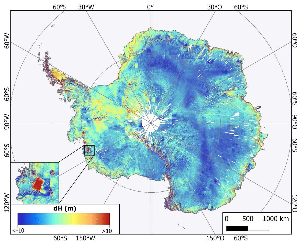
Figure 18 Height difference of TanDEM-X DEM minus REMA.

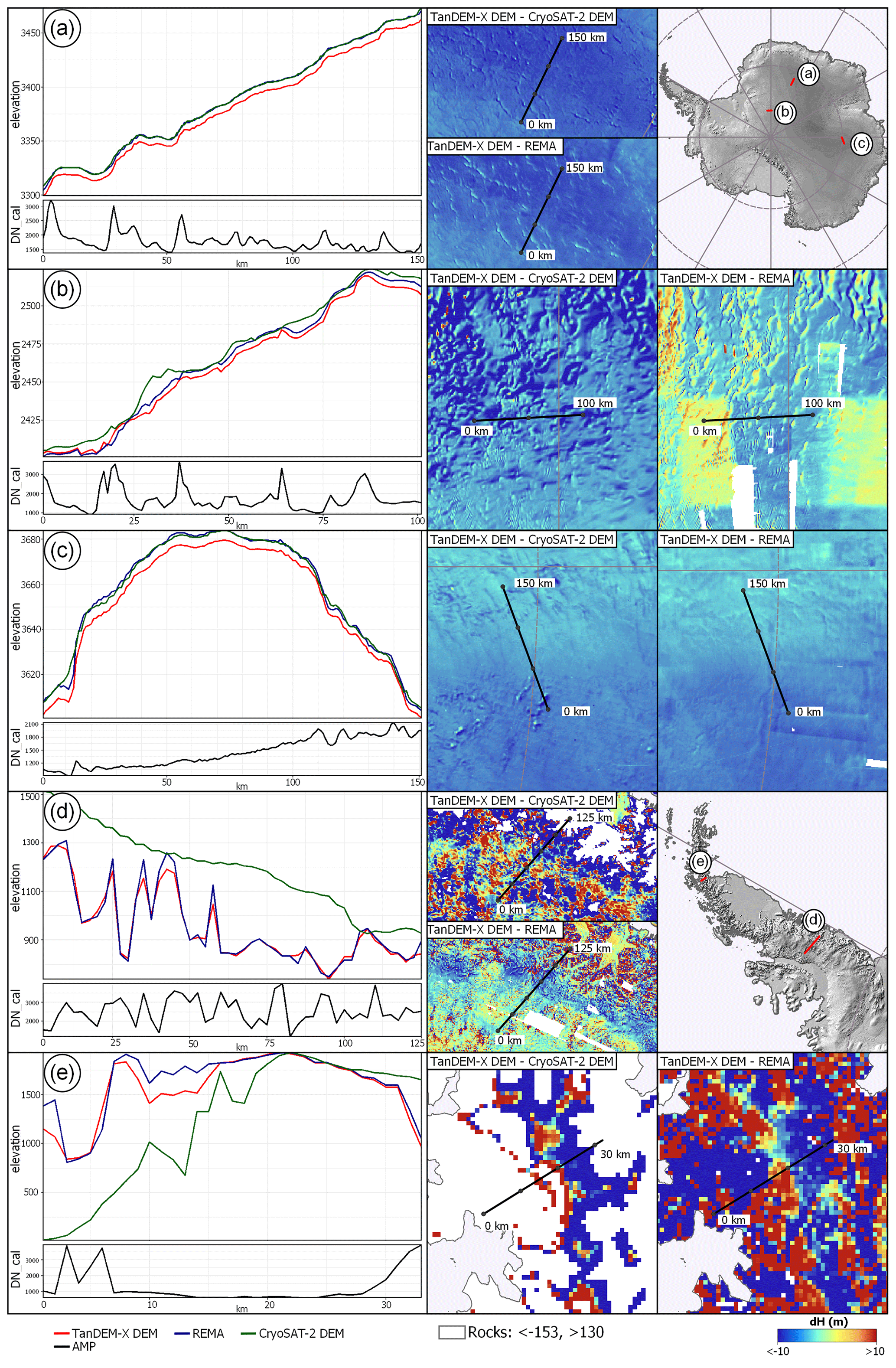
Figure 19 Left panels: profiles of TanDEM-X minus REMA, as well as minus CryoSat-2. Right panels: profile line plotted over the DEM differences.

Some consistent areas clearly stand out, like the Pine and Thwaites glaciers, where we have a quite good correspondence in height for this dynamic area. On the one hand, this is due to the close timing of the two dates, and on the other hand, the floating part of the ice shelf matches well where there is no penetration.

For a more detailed comparison of the different DEMs, we plotted elevation profiles of TanDEM-X, REMA, and CryoSat-2 for some key areas (Fig. 19). In the first profile (Fig. 19a), there is a relatively homogeneous penetration bias between TanDEM-X and REMA or CryoSat-2 except for some crevasses. The profiles in Fig. 19b, d, and e illustrate the capability of the DEMs to capture fine-scale topography and their limitations especially in the case of the 1 km data set of CryoSat-2. In the difference images of TanDEM-X minus REMA in Fig 19b and c, some rectangular features from the REMA DEM can be observed where REMA is close to or even below TanDEM-X DEM.

In summary, due to the high vertical resolution and coverage, so far undetected errors in TanDEM-X PolarDEM could be revealed by REMA. CryoSat-2 DEM and REMA are both highly accurate and therefore allow for an error characterization of the data set.

6 Conclusions and outlook

The TanDEM-X PolarDEM of Antarctica is a new interferometric DEM data set freely available to scientific users in 90 m horizontal spacing. It is void-free, and only the elevations of a few islands are missing on the Antarctic Peninsula. A new DEM calibration approach, additional acquisitions, and new editing techniques were utilized to shape the global TanDEM-X DEM into the new TanDEM-X PolarDEM 90 m product. In particular, the interferometric DEM was validated with blue ice areas that seem to be free of penetration effects. The corresponding accuracy measures are close to the absolute accuracy measures found by validation with highly accurate GPS tracks on other continents (Wessel et al., 2018). The quality of the data in terms of absolute vertical accuracy, evaluated by comparing the TanDEM-X DEM to ICESat heights, delivered a very good performance with a median value of −0.32 m and an absolute height accuracy at 90 % confidence level of 3.74 m on blue ice regions. Including the whole of Antarctica, also rock and snow/firn areas which are characterized mainly by radar wave penetration phenomena, the overall mean is −3.22 m with a standard deviation of ±2.56 m. The conducted DEM calibration was designed to preserve the SAR signal penetration into the ice sheet. Aside from the subsurface, the InSAR DEM captures local and regional relief quite well, as evidenced by the well-matching local heights with REMA DEM.

In cryosphere applications, different SAR sensors are well established and widely used. They all have in common that the SAR signal penetrates and the derived information is not related purely to the upper surface. Therefore, the TanDEM-X DEM could serve as an ideal basis DEM, e.g., for applications like the interferometric SAR velocity estimation and also the orthorectification of SAR data. They benefit from a similar penetration bias, as well as from a complete, gap-free coverage, which is a prerequisite for these applications. For DEM to DEM comparison, the penetration bias should be handled adequately. For example, Huber et al. (2020) used the TanDEM-X DEM of Greenland in a comparison with aerial photogrammetric DEMs over a 28-years period and therefore decided to neglect the penetration. In contrast, Malz et al. (2018) used the TanDEM-X DEM for a comparison with Shuttle Radar Topography Mission (SRTM) and roughly estimated the different penetration biases in advance. In both cases, the (residual) unknown penetration bias was regarded and modeled as an additional uncertainty for the heights as it comprises just a few meters. For X-band DEM to X-band DEM comparisons the penetration bias could be regarded as an uncertainty assuming similar biases (Floricioiu et al., 2016). A further refinement of this data set might be possible by correcting the penetration bias, as shown, for example, by Abdullahi et al. (2019) on the basis of coherence and amplitude or by Rott et al. (2021) on the basis of the interferometric volume correlation coefficient, which would improve the comparability with other data. An adequate handling of individual height offset scenes like in Dong et al. (2021) and a re-calibration near the Antarctic Peninsula down to Getz glacier could lead to a further improvement of this data set. Also, the amplitude mosaic itself could be further exploited in a more detailed analysis and in comparison with other backscatter data, e.g., RADARSAT or ERS-$\mathrm{1}/\mathrm{2}$ at C-band or PALSAR-2 at L-band. All in all, TanDEM-X PolarDEM is a framework for the provision of derivatives of the global digital elevation model of the TanDEM-X mission which resolved some limitations, including edited DEM products. Single year coverages and penetration-bias-corrected DEMs of polar regions will be supplemented in the future, especially over Greenland. Besides its good absolute accuracy this edited TanDEM-X PolarDEM 90 m product for Antarctica provides a high level of detail. It serves as a new topographic reference from which the monitoring of the dynamic topographic changes in Antarctica will benefit.

Appendix A: Product description

The global DEM delivered by TanDEM-X has been defined in the TanDEM-X DEM product specification document (Wessel, 2018). In contrast to this, the gap-filled and edited TanDEM-X PolarDEM 90 m of Antarctica introduced in this paper is described by the following parameters (Huber, 2020):

• projection: WGS 84/Antarctic Polar Stereographic;

• EPSG: 3031;

• vertical datum: WGS-84G1150 (ITRF2008 and ITRF2010);

• height reference: ellipsoidal heights;

• elevation unit: meters;

• grid spacing: 90 m;

• coverage: all land masses below 60^∘ S in four tiles;

• acquisition dates: mainly April 2013 to October 2014 (for gap filling July 2016 to September 2017);

• data format: 32 bit signed float;

• no data value: −32767.0;

• license: TanDEM-X PolarDEM 90 m for Antarctica is licensed for scientific use.