Assimilating near-real-time mass balance stake readings into a model ensemble using a particle filter

Short-term glacier variations can be important for water supplies or hydropower production, and glaciers are important indicators of climate change. This is why the interest in near-real-time mass balance nowcasting is considerable. Here, we address this interest and provide an evaluation of continuous observations of point mass balance based on online cameras transmitting images every 20 min. The cameras were installed on three Swiss glaciers during summer 2019, provided 352 near-real-time point mass balances in total, and revealed melt rates of up to 0.12 m water equivalent per day ($\mathrm{m}\mathrm{w}.\mathrm{e}.{\mathrm{d}}^{-\mathrm{1}}$) and of more than 5 $\mathrm{m}\mathrm{w}.\mathrm{e}.$ in 81 d. By means of a particle filter, these observations are assimilated into an ensemble of three TI (temperature index) and one simplified energy-balance mass balance models. State augmentation with model parameters is used to assign temporally varying weights to individual models. We analyze model performance over the observation period and find that the probability for a given model to be preferred by our procedure is 39 % for an enhanced TI model, 24 % for a simple TI model, 23 %, for a simplified energy balance model, and 14 % for a model employing both air temperature and potential solar irradiation. When compared to reference forecasts produced with both mean model parameters and parameters tuned on single mass balance observations, the particle filter performs about equally well on the daily scale but outperforms predictions of cumulative mass balance by 95 %–96 %. A leave-one-out cross-validation on the individual glaciers shows that the particle filter is also able to reproduce point observations at locations not used for model calibration. Indeed, the predicted mass balances is always within 9 % of the observations. A comparison with glacier-wide annual mass balances involving additional measurements distributed over the entire glacier mostly shows very good agreement, with deviations of 0.02, 0.07, and 0.24 $\mathrm{m}\mathrm{w}.\mathrm{e}.$

1 Introduction

Glaciers around the world are shrinking. For example, Switzerland has lost already more than a third of its glacier volume since the 1970s (Fischer et al., 2015), glaciers are currently melting at about −0.6 $\mathrm{m}\mathrm{w}.\mathrm{e}.{\mathrm{a}}^{-\mathrm{1}}$ (water equivalent per year) on average (Sommer et al., 2020), and it is expected that glaciers will continue to lose mass (Jouvet et al., 2011; Salzmann et al., 2012; Beniston et al., 2018; Zekollari et al., 2019). Since glaciers are important for the supply of drinking water or for irrigation and electricity production, there is high interest in near-real-time glacier mass balance information. Such information has also become important in the context of public outreach, e.g., for demonstrating the consequences of climate change (e.g., Euronews, 2019; Science Magazine, 2019).

A glacier mass balance nowcasting framework assimilating relevant observations could deliver these near-real-time mass balances whenever required. While nowcasting frameworks exist, for example, for the mass balance of the Greenland Ice Sheet (Fettweis et al., 2013; NSIDC, 2020a), for snow (NSIDC, 2020b; SLF, 2020) or for hydrological purposes (Zappa et al., 2008; Pappenberger et al., 2016; Zappa et al., 2018; WSL, 2020; Hydrique, 2020; Wu et al., 2020), there is no specific framework providing such analyses for mountain glaciers yet. In general, data assimilation is widespread in oceanography, meteorology, hydrology, and snow sciences, “but its introduction in glaciology is fairly recent” (Bonan et al., 2014). Especially regarding glacier mass balance studies, data assimilation and Bayesian approaches have appeared only slowly in published work (Dumont et al., 2012; Leclercq et al., 2017; Rounce et al., 2020; Werder et al., 2020).

In many cases, mass balance analyses are available twice a year and are based on seasonal in situ observations (Cogley et al., 2011). This relatively low frequency is related to the fact that in situ observations are expensive in terms of both time and manpower. Only recently have low-cost and high-frequency monitoring approaches emerged (Hulth, 2010; Fausto et al., 2012; Keeler and Brugger, 2012; Biron and Rabatel, 2019; Carturan et al., 2019; Gugerli et al., 2019; Netto and Arigony-Neto, 2019). However, even with these observations, it is not straightforward to provide analyses at higher frequencies. This is because near-real-time estimates are often based on ensemble modeling in order to enable a correct quantification of uncertainties. Ensemble modeling is used in glaciology in the context of model intercomparison projects (Hock et al., 2019), future projections for ice sheets and mountain glaciers (e.g., Ritz et al., 2015; Shannon et al., 2019; Golledge, 2020; Marzeion et al., 2020; Seroussi et al., 2020), and also determining the initial conditions for modeling (Eis et al., 2019). However, ensembles are currently not prominent in the calculation of seasonal or daily glacier mass balances. Another reason why calculating higher-frequency glacier mass balance analyses is not straightforward is the lack of knowledge about the short-term variability in the parameters of the necessary models. Temperature index (TI) models, for example, are parametrizations of the full energy balance equation, and they offset some of the changes occurring in the driving processes through parameter fluctuations (Ohmura, 2001; Lang and Braun, 1990; Hock, 2003; Hock et al., 2005). In a comparison of four TI models and a full energy balance model, Gabbi et al. (2014) showed that all models perform very similarly on a multi-year scale.

In this study, we address the issue of low-frequency observations, ensemble modeling, and the lack of knowledge about short-term parameter variability as part of the project CRAMPON (Cryospheric Monitoring and Prediction Online). The latter aims at delivering near-real-time glacier mass balance estimates for mountain glaciers using data assimilation. To obtain high-frequency data at a relatively low cost, we equipped three Swiss glaciers – Glacier de la Plaine Morte, Findelgletscher, and Rhonegletscher – with seven cameras in total. The cameras were operated in summer 2019 and took images of a mass balance stake marked every 2 cm at 20 min intervals, thus providing estimates of surface point mass balance aggregated to the daily scale. By using a particle filter (e.g., Arulampalam et al., 2002; Beven, 2009; Magnusson et al., 2017), we assimilate these observations into an ensemble of three TI models and one simplified energy balance model.

Ensemble stability and suitability for operational use is ensured by designing the particle filter such that, at any instance, each model has a minimum contribution to the mass balance model ensemble. In particular, models with temporarily bad performance are not excluded from the ensemble and can thus regain weight later. To address parameter uncertainty, we drive the mass balance model ensemble with both Monte Carlo samples of uncertain meteorological input and prior parameter distributions obtained from calibration to past, longer-term seasonal mass balance series. By using an augmented state formulation of the particle filter, we constrain model parameters as well (e.g., Ruiz et al., 2013). We are not aware of glacier mass balance studies that have applied a multi-model ensemble based on a particle filter with the resampling methods we propose, although multi-model particle filters have been used for other applications (e.g., Kreucher et al., 2004; Ristic et al., 2004; Saucan et al., 2013; Wang et al., 2016).

As a result, we demonstrate (1) how a workflow including daily melt observations, ensemble modeling, and data assimilation works in practice, (2) to what extent the assimilated mass balances are able to reproduce cumulative observations, and (3) how the ensemble performs with respect to both reference forecasts and seasonal analyses from in situ measurements.

2 Study sites, data, and field instrumentation

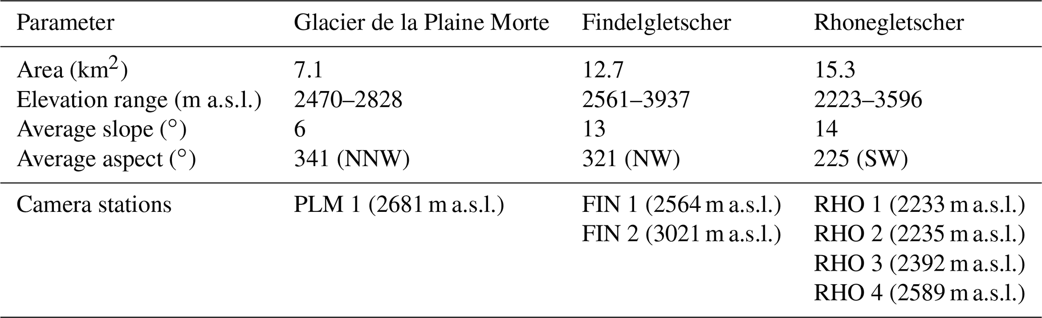
We use Glacier de la Plaine Morte, Rhonegletscher, and Findelgletscher in summer 2019 as test sites (Fig. 1). The basic morphological characteristics and instrumentations of these glaciers are given in Table 1.

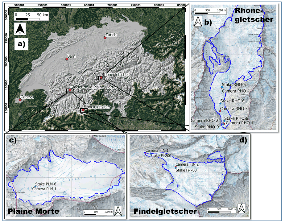
Figure 1 (a) Locations of the glaciers equipped with cameras within Switzerland and (b–d) detailed topographic maps of the glaciers with dots for cameras (red) and reference mass balance stakes (blue). Coordinates are given as Swiss coordinates (EPSG:21781). The blue glacier outlines stem from GLAMOS (Glacier Monitoring Switzerland), and background web mapping service tiles are provided by © swisstopo and © Google Maps.

Table 1 Main characteristics and installed cameras for the investigated glaciers. Glacier area and elevation range refer to the year 2019 (GLAMOS, 2020), and slope and aspect have been calculated using a recent DEM (digital elevation model) (swisstopo, 2020).

2.1 Continuous in situ mass balance observations

2.1.1 Technical camera station setup

For acquiring daily point mass balances in the field, we use off-the-shelf cameras and logger boxes from the company Holfuy Ltd. We mount the cameras to a construction of aluminum stakes that we designed for glacier applications. Figure 2 provides an overview of the camera installation.

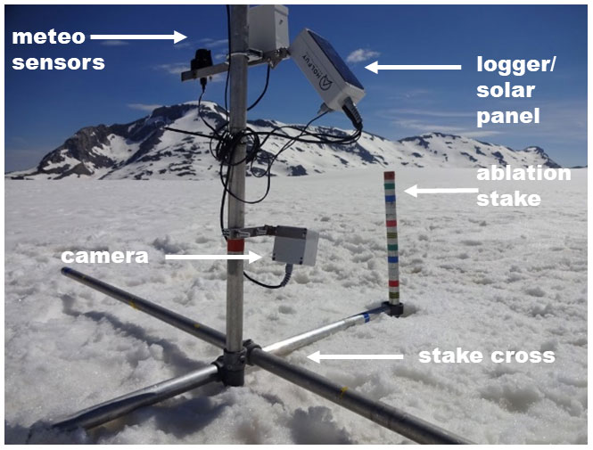
Figure 2 The camera setup used to obtain daily estimates of glacier point mass balance. Here, the camera has just been mounted on the snow-covered surface of Glacier de la Plaine Morte (19 June 2019).

The camera observes an ablation stake, which is marked with colored tape at 2 cm intervals. When the surface melts, the aluminum construction holding the camera slides along the mass balance stake. Pictures are taken every 20 min and are sent in real-time to our servers via the Swiss mobile phone network. Differences between subsequent pictures are used to infer daily glacier surface height changes relative to the stake top, which are the basis for ablation measurements (Cogley et al., 2011). All pieces of the construction are lightweight (4 kg for the station plus 4 kg for 8 m of mass balance stakes) and can be mounted by one person.

2.1.2 Camera acquisitions in summer 2019

Figure 3 shows an overview of camera acquisitions and data gaps over the summer 2019.

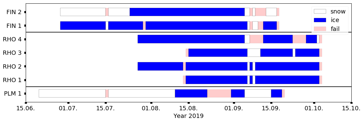
Figure 3 Overview of camera station availability during summer 2019. Cameras have been mounted and torn down at different times due to weather and staff restrictions. Station names are defined in Table 1. The category “snow” means that the glacier surface is snow covered, “ice” indicates that bare ice is exposed, and “fail” indicates either a failure in image transmission, station maintenance, or the inability to read the mass balance.

In total, we obtained 352 daily point mass balance observations between 20 June 2019 and 3 October 2019. The camera longest in the field was on Glacier de la Plaine Morte (91 d between 20 June 2019 and 18 September 2019), while those shortest in the field were two cameras at the tongue of Rhonegletscher (52 d between 13 August 2019 and 2 October 2019). Very few data gaps occurred due to failure of the mobile network over which the data were transmitted.

Once camera images are on our servers, they are read manually to obtain daily cumulative surface height change h(t,z) since camera setup. We assume that the observational error ϵ_t of a reading is Gaussian distributed and uncorrelated in time and space. To estimate the standard deviation of the Gaussian error distribution, we performed a round-robin experiment with seven participants. In this kind of experiment all participants were given the task to read h(t,z) from the same camera images independently, and statistics were made about the degree of agreement between the readings. We found a standard deviation of 1.5 cm, with a range from 0.2 to 1.7 cm. The estimate accounts for reading errors, errors in stake marker positions, and unknown thickness of the melt crust on the ice surface, but it does not account for systematic errors.

The relationship between observations of surface height change since an initial point in time (in our case the time at which a camera is set up) and the cumulative glacier mass balance is given through the simple linear observation operator ℋ:

$$\begin{array}{}\text{(1)}& h(t,z)=\mathcal{H}\left(b_{\mathrm{sfc}}\right(t,z\left)\right)+{\mathit{ϵ}}_{t,z}={\displaystyle \frac{b_{\mathrm{sfc}}(t,z)\cdot {\mathit{\rho }}_{\mathrm{w}}}{{\mathit{\rho }}_{\mathrm{bulk}}}}+{\mathit{ϵ}}_{t,z},\end{array}$$

where b_sfc(t,z) ($\mathrm{m}\mathrm{w}.\mathrm{e}.$) is the accumulated surface mass change at elevation z and time t since the day of the first camera observation, ρ_w=1000 kg m⁻³ is the water density, and ρ_bulk is the temporally weighted bulk density of snow and ice at the camera location (kg m⁻³). We expect the observation errors to be uncorrelated in time, since every reading is independent from the previous one. To avoid systematic errors in the readings, we exclude the initial, snow-covered phase after camera setup at stations FIN 2 and PLM 1. This is because the camera construction can sink into the snow cover, potentially biasing the snowmelt signal. This “sinking bias” is virtually impossible to distinguish from the actual melt signal. Moreover, the temporally varying density of the melting snow is unknown. Short snow events during the melt season are assigned a density of 150 kg m⁻³. The calculated snow water equivalent is assigned an uncertainty of 2–3 cm w.e. If a stake reading was impossible, we have resumed with a zero balance after the snowfall melted again. For days without snow, there are three cases that require special attention when reading mass balances: (1) maintenance operations like setup, redrilling, and unmounting of a station, (2) melt that happens during night and that is thus only visible on the next day, and (3) data gaps. Regarding maintenance operations (point “(1)”), we do not consider the observations from days when maintenance has taken place. This is either because those days are not fully covered or because the mass balance stake and the entire station might melt into the ice after redrilling. For nighttime melting (i.e., “(2)”), we equally distribute the overnight melt between the 2 d concerned. This is a trade-off between warmer temperatures before midnight and colder temperatures but longer time span after midnight. For data gaps (point “(3)”), we experienced only short image transmission outages which were mainly due to a 6 d failure in the mobile network connection on Plaine Morte during September 2019. We excluded the daily readings on these days but were able to reconstruct estimates of cumulative mass balance over the time gaps when acquisitions resumed.

2.2 Meteorological input data

To model glacier mass balance, we employ verified products of daily mean and maximum 2 m temperature T and T_max, precipitation sum P, and mean incoming shortwave radiation G from MeteoSwiss as model input (MeteoSwiss, 2018, 2021a, b). These are delivered on grids with approx. 0.2^∘ spatial resolution, which for Switzerland corresponds to a horizontal resolution of about 2 km.

Temperature uncertainty, given as a root-mean-square error, varies per season from 0.94 K (May to March) to 1.67 K (December to February) in the Alpine region (Frei, 2014; Christoph Frei, personal communication, 2020). We assume a Gaussian-distributed additive error perfectly correlated in space for a single glacier but independent on different days. The assumption of a perfect error correlation can be justified by the fact that the station network from which the gridded temperature values are interpolated is much sparser than the scale of individual glaciers. The air temperature lapse rate is derived from the 25 closest cells to a glacier outline centroid using a Bayesian estimation based on a linear regression model:

$$\begin{array}{}\text{(2)}& T_{t,i}=e_t+q_t{h}_i+{\mathit{\nu }}_{t,i},\end{array}$$

where T_t,i is the temperature of the ith grid cell out of the 25 considered cells at time t, e_t is the regression line intercept, q_t is the regression slope (i.e., $\frac{\partial T}{\partial z}$), h_i is the height of the ith grid cell, and ${\mathit{\nu }}_{t,i}\sim \mathcal{N}(\mathrm{0},{\mathit{\sigma }}_{\mathit{\nu },t}^{\mathrm{2}})$ are the residuals independent in space and time. Using a g-prior of Zellner (Zellner, 1986), being non-informative in the intercept e_t and model noise variance ${\mathit{\sigma }}_{\mathit{\nu },t}^{\mathrm{2}}$ of the regression, we draw samples of the lapse rate q_t from the following posterior distribution:

$$\begin{array}{}\text{(3)}& p(q_t\mid T_t)\propto {\left(\mathrm{1}+{\displaystyle \frac{{\left(q_t-\frac{g}{\mathrm{1}+g}\widehat{q_t}-\frac{\mathrm{1}}{\mathrm{1}+g}{q}_{\mathrm{0}}\right)}^{\mathrm{2}}}{\mathrm{24}{c}^{\mathrm{2}}}}\right)}^{-\mathrm{25}/\mathrm{2}}\end{array}$$

with

$$\begin{array}{}\text{(4)}& \begin{array}{rl}{c}^{\mathrm{2}}& ={\displaystyle \frac{g}{\mathrm{24}(\mathrm{1}+g)\sum (h_i-\overline{h}{)}^{\mathrm{2}}}}\\ & \cdot \left(s_t^{\mathrm{2}}+{\displaystyle \frac{\mathrm{1}}{\mathrm{1}+g}}\sum _i(h_i-\overline{h}{)}^{\mathrm{2}}(\widehat{q_t}-q_{\mathrm{0}}{)}^{\mathrm{2}}\right).\end{array}\end{array}$$

Above, p(⋅) means “probability of”, g determines a weighting factor composing the posterior mean (we set g=1), $\widehat{q_t}$ is the least squares estimator of the slope, q₀ is the prior mean, which we choose to be an annually varying climatological mean gradient at the respective grid location, $\overline{h}$ is the average height of the 25 grid cells, and $s_t^{\mathrm{2}}$ is the residual sum of squares. This is, up to a constant, the probability density of a t-distributed random variable with 24 degrees of freedom, shifted by $\frac{(g\widehat{q_t}+q_{\mathrm{0}})}{(\mathrm{1}+g)}$ and multiplied by c. The samples drawn from this distribution are then propagated into the particle filter.

For operational reasons, the precipitation grids contain the 06:00–06:00 local time precipitation sums and thus do not conform with the 00:00–00:00 temperature values (Isotta et al., 2019; MeteoSwiss, 2021b). This might introduce an error, which we cannot quantify. As for temperature, we thus focus again on random errors and pretend for simplicity that the precipitation sum was also from 00:00–00:00. Precipitation uncertainty is generally harder to assess than temperature uncertainty since it involves undercatch errors and skew error distributions. Here, we follow the error assessment by quantiles of precipitation intensity proposed by Isotta et al. (2014) and Christoph Frei, personal communication (2020), who calculated that, for the Alpine region, the standard error at moderate precipitation intensities roughly corresponds to an over- or underestimation by a factor of 1.25. The error increases (decreases) towards low (high) precipitation intensities, and it is generally slightly higher in the summertime. We draw samples from a multiplicative Gaussian error distribution and for the same reason as for temperature, we assume perfect precipitation error correlation at the glacier scale. We also derive Bayesian precipitation lapse rates from the surrounding 25 grid cells in the same fashion as we do for the temperature lapse rate. However, to circumvent high errors in the slope calculation due to the boundedness of precipitation towards zero, we (1) calculate the slope on the square root of the precipitation and (2) assign a probability that the reference has actually received precipitation when the reference cell value is zero but other cells have non-zero precipitation.

Shortwave radiation is derived using data from the geostationary satellite series Meteosat. As an uncertainty, Stöckli (2013) gives a mean absolute bias between 9 and 29 W m⁻². We assume the errors to be Gaussian and assign a standard deviation of 15 W m⁻², perfectly correlated on the glacier scale and independent in time. Shortwave radiation is downscaled from the grid to the glacier with potential radiation (see Sect. 3.1).

2.3 Glacier outlines and measured mass balances

Glacier outlines for the year 2019 are obtained from GLAMOS (Glacier Monitoring Switzerland), and mass balances are calculated over a fixed glacier surface area (Elsberg et al., 2001; Huss et al., 2012).

For calibration and verification, we use mass balance data acquired in the frame of GLAMOS (Glacier Monitoring Switzerland, 2018). First, intermediate stake readings independent from our near-real-time stations but close to our installations have been made explicitly for this study. Stake locations are depicted in Fig. 1. The reading error for these measurements is usually estimated to be around 5 cm (e.g., Müller and Kappenberger, 1991). Second, we use seasonal, glacier-wide mass balances based on in situ observations. These observations are acquired during two field campaigns in April and September, respectively. Glacier-wide mass balances are obtained by extrapolating the in situ observations and making the extrapolated values consistent with long-term mass changes. The latter procedure is sometimes referred to as “homogenization” (e.g., Bauder et al., 2007; Huss et al., 2015). For recent years, this homogenization has not been performed since no geodetic mass balances are available yet. The extrapolation method used to infer glacier-wide mass balance from point measurements involves an adjustment of the model parameters of an accumulation and TI melt model (Hock, 1999) at locations where observations are available, while mass balances at grid cells without observations are produced using the calibrated model (Huss et al., 2009, 2015). Uncertainties of the glacier-wide annual mass balance for the measurement period have been estimated to be 0.09–0.2 $\mathrm{m}\mathrm{w}.\mathrm{e}.$ in six experiments in which GLAMOS (1) model parameters (temperature lapse rate, ratio between melt coefficients, summer precipitation correction) and (2) snow extrapolation parameters have been varied within prescribed ranges and for which (3) mass balance stake reading uncertainty, (4) DEM (digital elevation model) and outline uncertainty, (5) climate forcing uncertainty, and (6) point data availability have been accounted.

3 Methods

3.1 Mass balance modeling

Glacier surface mass balance consists of two components: accumulation and ablation. We model accumulation and ablation on elevation bins whose vertical extent is determined by a ≈20 m horizontal spacing of nodes along the central flow line of the glacier (Maussion et al., 2019). To obtain glacier-wide mass balance, node mass balances are weighted with the area per elevation bin. To compute accumulation at different elevations, we employ a simple but widely used accumulation model (e.g., Huss et al., 2008):

$$\begin{array}{}\text{(5)}& c_{\mathrm{sfc}}(t,z)={\text{prcp}}_{\mathrm{scale}}\left(t\right)\cdot P_{\text{s}}\left(t\right)\cdot \left[\mathrm{1}+(z-z_{\mathrm{ref}})\cdot {\displaystyle \frac{\partial P_{\text{s}}}{\partial z}}\right],\end{array}$$

where c_sfc(t,z) ($\mathrm{m}\mathrm{w}.\mathrm{e}.$) is the snow accumulation at time step t and elevation z, prcp_scale(t) is the unitless multiplicative precipitation correction factor, P_s(t) is the sum of solid precipitation at the elevation of the precipitation reference cell z_ref and time step t, and $\frac{\partial P_{\text{s}}}{\partial z}$ is the solid precipitation lapse rate. Following Sevruk (1985), we choose prcp_scale to vary sinusoidally by ±8 % around its mean during 1 year, being highest in winter and lowest in summer. This is to account for systematic variations in gauge undercatch depending on the precipitation phase. The water phase change in the temperature range around 0 ^∘C is modeled using a linear function between 0 and 2 ^∘C; i.e., at 1 ^∘C there is 50 % snow and 50 % rain (e.g., Maussion et al., 2019).

Since all three glaciers we investigate are in the GLAMOS measurement program and winter mass balance observations are available, the effect of spatial variations in snow accumulation differing from a linear gradient can be incorporated. This is done by choosing a factor D(z) such that the model mass balance in the elevation bins matches the measured and interpolated distribution of the winter mass balance (Farinotti et al., 2010):

$$\begin{array}{}\text{(6)}& C_{\mathrm{sfc},\mathrm{glamos}}^{\mathrm{w}}\left(z\right)=D\left(z\right)\cdot C_{\mathrm{sfc}}^{\mathrm{w}}\left(z\right).\end{array}$$

Here, $C_{\mathrm{sfc}}^{\mathrm{w}}\left(z\right)$ ($\mathrm{m}\mathrm{w}.\mathrm{e}.$) is the modeled winter surface accumulation, i.e., the sum of individual c_sfc(t,z) over the winter period, and $C_{\mathrm{sfc},\mathrm{glamos}}^{\mathrm{w}}\left(z\right)$ ($\mathrm{m}\mathrm{w}.\mathrm{e}.$) is the interpolated winter surface accumulation at elevation z.

To model surface ablation, we set up an ensemble of three TI melt models and one simplified energy-balance melt model. We choose this ensemble since the individual models differ in the degree of complexity by which they describe the surface energy balance (Hock, 2003). The models range from using only temperature as input for determining melt via employing additionally the potential irradiation to using temperature and the actual shortwave radiation. The ensemble contains the following:

1. The “BraithwaiteModel” uses only air temperature as input to calculate melt (Braithwaite and Olesen, 1989; Braithwaite, 1995):

   $$\begin{array}{}\text{(7)}& a_{\mathrm{sfc}}(t,z)={\text{DDF}}_{\mathrm{snow}/\mathrm{ice}}\cdot max\left(T\right(t,z)-T_{\mathrm{melt}},\mathrm{0}),\end{array}$$

   where a_sfc(t,z) ($\mathrm{m}\mathrm{w}.\mathrm{e}.{\mathrm{d}}^{-\mathrm{1}}$) and T(t,z) (^∘C) are surface ablation and air temperature at time step t and elevation z, respectively, ${\text{DDF}}_{\mathrm{snow}/\mathrm{ice}}$ ($\mathrm{m}\mathrm{w}.\mathrm{e}.{\mathrm{K}}^{-\mathrm{1}}{\mathrm{d}}^{-\mathrm{1}}$) are the temperature sensitivities (“degree-day factors”) of the surface types (snow and ice), max() is the maximum operator, and T_melt (^∘C) is the threshold temperature for melt. For this application, we set T_melt to 0 ^∘C and keep the ratio of ${\text{DDF}}_{\mathrm{snow}}/{\text{DDF}}_{\mathrm{ice}}$ constant at 0.5 (Hock, 2003).

2. The “HockModel” uses potential incoming solar radiation as an additional predictor for melt (Hock, 1999):

   $$\begin{array}{}\text{(8)}& \begin{array}{rl}{a}_{\mathrm{sfc}}(t,z)& =(\text{MF}+a_{\mathrm{snow}/\mathrm{ice}}\cdot I_{\mathrm{pot}}(t,z\left)\right)\\ & \cdot max\left(T\right(t,z)-T_{\mathrm{melt}},\mathrm{0}),\end{array}\end{array}$$

   where MF ($\mathrm{m}\mathrm{w}.\mathrm{e}.{\mathrm{K}}^{-\mathrm{1}}{\mathrm{d}}^{-\mathrm{1}}$) is the temperature melt factor, $a_{\mathrm{snow}/\mathrm{ice}}$ ($\mathrm{m}\mathrm{w}.\mathrm{e}.{\mathrm{m}}^{\mathrm{2}}{\mathrm{d}}^{-\mathrm{1}}{\mathrm{W}}^{-\mathrm{1}}{\mathrm{K}}^{-\mathrm{1}}$) are the radiation coefficients for snow and ice, respectively, I_pot(t,z) (W m⁻²) is the potential clear-sky direct solar radiation at time t and elevation z, T_melt is set again to 0 ^∘C, and the ratio of $a_{\mathrm{snow}}/a_{\mathrm{ice}}$ is 0.8 (Hock, 1999; Farinotti et al., 2012). I_pot(t,z) is computed at 10 min intervals following the methods described in Iqbal (1983), Hock (1999), and Corripio (2003) and by using swissALTI3D (swisstopo, 2020) as a background elevation model. Daily values are then obtained by averaging these values, and values for the different glacier elevations are aggregated. We assume equal uncertainties for both actual and potential incoming shortwave radiation G and I_pot.

3. The “PellicciottiModel” employs surface albedo and actual incoming shortwave solar radiation (Pellicciotti et al., 2005):

   $$\begin{array}{}\text{(9)}& a_{\mathrm{sfc}}(t,z)=\left\{\begin{array}{l}\text{TF}\cdot T(t,z)+\text{SRF}\cdot (\mathrm{1}-\mathit{\alpha }(t,z\left)\right)\\ \cdot G(I_{\mathrm{pot}},t,z),\text{for }T(t,z)>T_{\mathrm{melt}}\\ \mathrm{0},\text{for }T(t,z)\le T_{\mathrm{melt}}\end{array}\right.,\end{array}$$

   where TF ($\mathrm{m}\mathrm{w}.\mathrm{e}.{\mathrm{K}}^{-\mathrm{1}}{\mathrm{d}}^{-\mathrm{1}}$) is the temperature factor, SRF (${\mathrm{m}}^{\mathrm{3}}{\mathrm{d}}^{-\mathrm{1}}{\mathrm{W}}^{-\mathrm{1}}$) is the shortwave radiation factor, and α(t,z) and $G(I_{\mathrm{pot}},t,z)$ (W m⁻²) are the albedo and incoming shortwave radiation at time t and elevation z, respectively. Note that in this case, T_melt=1 ^∘C (Pellicciotti et al., 2005).

   Albedo is approximated according to the combined decay equation for deep and shallow snow in Brock et al. (2000):

   $$\begin{array}{}\text{(10)}& \begin{array}{rl}\mathit{\alpha }(t,z)& =(\mathrm{1}-e^{(-\text{swe}(t,z)/{\text{swe}}^{*})})\\ & \cdot (p_{\mathrm{1}}-p_{\mathrm{2}}\cdot {\log }_{\mathrm{10}}(T_{\mathrm{acc}}(t,z)\left)\right)\\ & +e^{(-\text{swe}(t,z)/{\text{swe}}^{*})}\cdot \left({\mathit{\alpha }}_u\right(t,z)\\ & +p_{\mathrm{3}}\cdot e^{-p_{\mathrm{4}}\cdot T_{\mathrm{acc}}(t,z)}),\end{array}\end{array}$$

   where swe(t,z) is the snow water equivalent at time t and elevation z, ${\text{swe}}^{*}=\mathrm{0.024}\mathrm{m}\mathrm{w}.\mathrm{e}.$ is a scaling length for swe, p₁=0.713, p₂=0.155, p₃=0.442, and p₄=0.058 are empirical coefficients as given in Brock et al. (2000), α_u is the albedo of the underlying firn/ice below the snow, and T_acc(t,z) is the accumulated daily maximum temperature >0 ^∘C since a snowfall event at elevation z. To avoid infeasible albedo values, α(t,z) is clipped as suggested in Brock et al. (2000).

4. The “OerlemansModel” calculates melt energy as the residual term of a simplified surface energy balance equation (Oerlemans, 2001):

   $$\begin{array}{}\text{(11)}& a_{\mathrm{sfc}}(t,z)={\displaystyle \frac{Q_{\text{m}}(t,z)\mathit{\delta }t}{L_f{\mathit{\rho }}_{\mathrm{w}}}},\end{array}$$

   where

   $$\begin{array}{}\text{(12)}& \begin{array}{rl}{Q}_{\text{m}}(t,z)& =(\mathrm{1}-\mathit{\alpha }(t,z\left)\right)\cdot G(I_{\mathrm{pot}},t,z)\\ & +c_{\mathrm{0}}+c_{\mathrm{1}}\cdot T(t,z).\end{array}\end{array}$$

   Here, Q_m(t,z) (W m⁻²) is the melt energy at time t and elevation z, δt=1 d is a time step, $L_f=\mathrm{3.34}\times {\mathrm{10}}^{\mathrm{5}}$ (J kg⁻¹) is the latent heat of fusion, and c₀ (W m⁻²) and c₁ ($\mathrm{W}{\mathrm{m}}^{-\mathrm{2}}{\mathrm{K}}^{-\mathrm{1}}$) are empirical factors. The albedo α is calculated as well according to Eq. (10).

3.2 Mass balance model calibration

For the data assimilation procedure described in Sect. 3.3, we need a prior estimate for the model parameter values of Eqs. (5), (7), (8), (9), and (12). To obtain this, we calibrate the three investigated glaciers against the GLAMOS glacier-wide mass balances (Sect. 2.3) and use an iterative procedure similar to Huss et al. (2009), illustrated in Fig. 4. Additionally, we calibrate the snow redistribution factor D(z) annually.

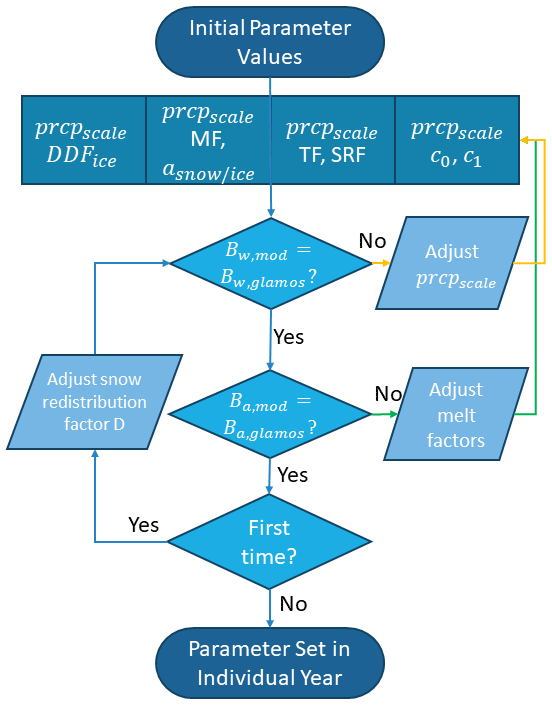
Figure 4 Calibration workflow used to obtain a prior estimate for the parameters of the model ensemble . B_x,mod and B_x,glamos are the modeled and GLAMOS glacier-wide mass balances, respectively, with x referring either to winter (w) or annual (a) values. The yellow arrows highlight the first iteration step, while the green arrows highlight the second iteration step. Figure altered from Huss et al. (2009).

Following Huss et al. (2009), all model parameters are initially set to values reported in the literature (Hock, 1999; Oerlemans, 2001; Pellicciotti et al., 2005; Farinotti et al., 2012; Gabbi et al., 2014), and a two-step calibration procedure is then applied: first, the precipitation correction factor is tuned so that the winter mass balance of a given year is reproduced. In this step, the melt factors are held constant at their initial values. In a second step, the calibrated precipitation factor is kept constant, and the melt factors are optimized to reproduce the annual mass balance. The two steps are repeated alternately, and both precipitation correction and melt factors converge with every iteration. We terminate the iteration after the absolute difference to the winter and annual mass balance drops below 1 $\mathrm{mm}\mathrm{w}.\mathrm{e}.$

Once the model parameters have been optimized, we determine the value of D(z) that matches the interpolated winter mass balance. Since this may result in changes in the required model parameters, the iterative procedure is applied one more time as a final step.

3.3 Particle filtering

To ensure that all mass balance model predictions stay within the observational uncertainty, we perform data assimilation. In particular, we employ a particle filter since it does not restrict the class of state transition models and error distributions. Especially when temperatures are around the melting point, the system becomes nonlinear since melt occurs above but not below this point. As a consequence, the distributions we deal with are not necessarily Gaussian. The facts that (a) the temperature chosen to parametrize the melting point is not the same for all four models, (b) the individual model prior distributions are combined to obtain the ensemble prediction, and (c) there can also be accumulation contributing to the overall mass balance add further complexity. We do not use other data assimilation approaches, such as variational methods or ensemble Kalman filtering, because variational methods encounter difficulties when dealing with non-Gaussian priors (van Leeuwen et al., 2019), whilst the ensemble Kalman filter in its original form is not designed for multi-model applications as we use in our case. Overall, particle filtering is a very flexible, generalizable, and readily implementable data assimilation method.

Some extensions of the common particle filter framework allow model parameters and model performance to be estimated over time. With this, we aim at providing optimal, daily mass balance estimates at the glacier scale.

3.3.1 General framework

The general framework for data assimilation consists of a system whose state x_t evolves according to a model, but only partial and uncertain observations y_t of the state are available.

$$\begin{array}{}\text{(13)}& \left\{\begin{array}{ll}{\mathit{x}}_t=g({\mathit{x}}_{t-\mathrm{1}},{\mathit{\beta }}_t),& \text{state transition equation}\\ {\mathit{y}}_t=\mathcal{H}\left({\mathit{x}}_t\right)+{\mathit{ϵ}}_t,& \text{observation equation}\end{array}\right.\end{array}$$

Here, x_t−1 is the state at the previous time step t−1, g(⋅) is the state transition function, ℋ is the observation operator as introduced in Eq. (1), ϵ_t is the observation error vector at time t, and β_t is a random variable that describes model uncertainties. The term for β_t does not need to be strictly additive, and it should include uncertainties stemming from the model input variables. The goal of data assimilation is to compute conditional distributions of the system state x_t based on observations ${\mathit{y}}_{\mathrm{1}:t}=({\mathit{y}}_{\mathrm{1}},{\mathit{y}}_{\mathrm{2}},\mathrm{\dots },{\mathit{y}}_t)$ sequentially for $t=t_{\mathrm{0}},t_{\mathrm{0}}+\mathrm{1},\mathrm{\dots }{t}_{\mathrm{end}}$, where t₀ and t_end are the time steps with the first and last observations, respectively. In our case, these conditional distributions describe the cumulative mass balance of a glacier, given all available camera observations.

To put this general framework into practice, we use the particle filter, which is a sequential Monte Carlo data assimilation method. Instead of handling conditional distributions of x_t analytically, the particle filter approximates the conditional distribution of a state x_t at time t given the observations y_1:t by a weighted sample of size N_tot (e.g., van Leeuwen et al., 2019).

$$\begin{array}{}\text{(14)}& p({\mathit{x}}_t\mid {\mathit{y}}_{\mathrm{1}:t})\approx \sum _{k=\mathrm{1}}^{N_{\mathrm{tot}}}{w}_{t,k}\mathit{\delta }({\mathit{x}}_t-{\mathit{x}}_{t,k}),\sum _{k=\mathrm{1}}^{N_{\mathrm{tot}}}{w}_{t,k}=\mathrm{1}\end{array}$$

Here δ(⋅) is the Dirac delta function, the elements x_t,k of the sample are called “particles”, and the weights w_t,k associated with the particles x_t,k sum to unity.

Usually, particle filtering comprises three repeated steps: the predict step, the update step, and the resampling step. In our case, these steps mean the following: during the predict step, particles holding possible mass balance states are propagated forward in time using the state transition in Eq. (13), where g(⋅) represents the ensemble prediction of mass balance Eqs. (5)–(10). This acts as a prior estimate of the mass balance distribution. In the update step, the weights of the propagated particles are recalculated based on Bayes' theorem. This accounts for the information of the next camera observation. In the last step, particles are resampled according to the updated weights. This step is necessary to restore particle diversity that is reduced during the update step. Resampling avoids so-called particle degeneracy, in which all weights collapse on only a few particles. Beyond the common three-step scheme, we additionally estimate model parameters with the particle filter by augmenting the state vector with model parameter values. In this way, we add an additional fourth step to the particle filter scheme, in which we evolve model parameters temporally according to a defined memory parameter. This prevents a collapse of the ensemble due to overconfidence, meaning that model parameter variability would become too low over time.

3.3.2 Application of the framework

The flowchart in Fig. 5 visualizes how the particle filter is implemented in our modeling framework. Figure 6 sheds light on how we perform the individual particle filter steps.

Figure 5 Particle filter workflow during 1 mass budget year (“MB year”). We use uncertain model estimates to predict mass balance with 10 000 particles and reset the cumulative mass balance when a camera is set up. The model mass balance estimate is updated at time steps for which observations are available. To avoid overconfidence of the particle filter, we apply a partial resampling technique. The individual particle filter steps are sketched in Fig. 6.

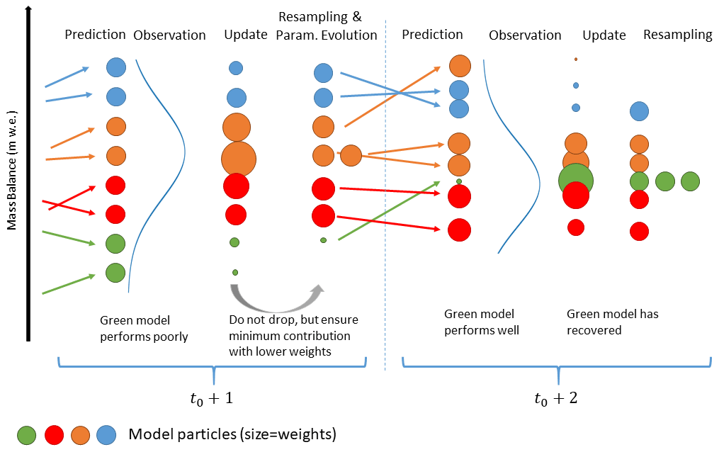
Figure 6 Illustration of the individual particle filter steps. The example refers to a case in which four models (blue, orange, red, and green) start with two particles each. The blue curve represents the observation distribution. At time step t₀+1, the green model performs poorly and receives entirely low weights during the update step (weights are shown by the size of the circles). In the resampling step, we modify the weights of the other particles again. This is for not omitting the green model entirely due to temporarily poor performance. As the green model stays in the ensemble, it can recover later, i.e., when making a good prediction (here: t₀+2).

The temporal dynamics of the glacier mass balance state can be described by the accumulation model in Eq. (5) combined with the four different melt models in Eqs. (7), (8), (9), and (11). A priori, it is not known which model performs best, and each model has a set of unknown parameters. To take these two uncertainties into account, we augment the state vector by the model index $m_t\in \mathit{\{}\mathrm{1},\mathrm{2},\mathrm{3},\mathrm{4}\mathit{\}}$ and the model parameters θ_t. In this way, a model weight and the model parameter values are also estimated based on the observations. Although the unknown parameters are different for each model, we do not use an additional model index for θ_t. Instead, we ensure that for all particles, θ_t,k is always the parameter vector associated with model m_t,k. This means that, when following a given particle backwards in time, its entire dynamics is governed by one single model only. In the forward direction, a particle can “die off” and be replaced by another particle with different model index. In this case, both the model index m_t,k and the entire past trajectory are changed to the new model.

As the state has to provide all information that is needed to predict the next observation, we also include the surface albedo and the snow water equivalent on the ice in our state vector. Hence, the state vector is defined as

$$\begin{array}{}\text{(15)}& {\mathit{x}}_t=(m_t,{\mathit{\theta }}_t,{\mathit{\xi }}_t),{\mathit{\xi }}_t=\left(b_{\mathrm{sfc}}\right(t,z),\mathit{\alpha }(t,z),\text{swe}(t,z\left)\right).\end{array}$$

Here, ξ_t is called the physical state.

3.3.3 Predict step

During the predict step, the explicit temporal evolution of the physical state ξ_t involves the randomized error accounting for uncertainties in the meteorological input (Sect. 2.2). Here, we call these errors η_t and set an additional scalar subscript to indicate that the errors are different for each meteorological variable. We first predict c_sfc(t,z), T_acc(t,z), and swe(t,z).

$$\begin{array}{}\text{(16)}& {\displaystyle }{c}_{\mathrm{sfc}}(t,z)=c_{\mathrm{sfc}}\left(P_{\text{s}}\right(t,z),{\mathit{\eta }}_{t,\mathrm{2}},{\mathit{\theta }}_t)\text{(17)}& {\displaystyle }{T}_{\mathrm{acc}}(t,z)=\left\{\begin{array}{l}{T}_{\mathrm{acc}}\left(\mathit{\alpha }\right(t-\mathrm{1},z\left)\right)+T_{\max }(t,z)+{\mathit{\eta }}_{t,\mathrm{1}},\\ \text{if }{T}_{\max }(t,z)>\mathrm{0}\text{ and }\\ c_{\mathrm{sfc}}(t,z)<\mathrm{0.001}\mathrm{m}\mathrm{w}.\mathrm{e}.{\mathrm{d}}^{-\mathrm{1}}\\ \mathrm{0},\text{otherwise.}\end{array}\right.\text{(18)}& {\displaystyle }\begin{array}{rl}\text{swe}(t,z)& =max\left(\text{swe}\right(t-\mathrm{1},z)-a_{\text{sfc}}(t-\mathrm{1},z),\mathrm{0})\\ & +c_{\mathrm{sfc}}(t,z)\end{array}\end{array}$$

Based on Eqs. (7), (8), (9), and (11), the predicted mass balance is then

$$\begin{array}{}\text{(19)}& \begin{array}{rl}{b}_{\mathrm{sfc}}(t,z)=& b_{\mathrm{sfc}}(t-\mathrm{1},z)\\ & +c_{\mathrm{sfc}}(t,z)\\ & -a_{\mathrm{sfc}}\left(T\right(t,z)+{\mathit{\eta }}_{t,\mathrm{3}},G(I_{\mathrm{pot}},t,z)\\ & +{\mathit{\eta }}_{t,\mathrm{4}},\mathit{\alpha }\left(T_{\mathrm{acc}}\right(t,z\left)\right),\text{swe}(t,z),m_t,{\mathit{\theta }}_t)\\ & +{\mathit{\beta }}_t,\end{array}\end{array}$$

where the errors η_t are independent in time but partly perfectly correlated in space for reasons described in Sect. 2.2. By introducing both the meteorological uncertainty η and the parameter uncertainties, we shift the majority of the uncertainty contained in β_t to these variables. Since the remaining uncertainty for β_t is small and hard to quantify, we set β_t=0 for simplicity. With this assumption, we neglect some additional uncertainty contained in β_t, being aware that this might lead to “jumps” in the temporal evolution of the model performance. Finally, the observations y_t depend only on the cumulative mass balance at the elevation z of the camera as specified in Eq. (1).

We use a total of N_tot=10 000 particles and set the weights at time t₀ (i.e., the time when the first camera observation is available) to $\mathrm{1}/N_{\mathrm{tot}}$. Since at t₀ all models have equal probabilities, $N_{\mathrm{tot}}/\mathrm{4}$ particles are assigned to each of the four models. The initial value of b_sfc(t₀,z) is set to zero for all particles, whereas α(t₀,z) is determined by the maximum air temperature since the last snowfall before t₀, and swe(t₀,z) depends on the cumulative mass balance before t₀. Finally, the initial calibration parameter values ${\mathit{\theta }}_{t_{\mathrm{0}},k}$ of the particles with model index j are obtained by drawing Monte Carlo samples from a normal distribution fitted to the logarithmized parameters of model j, as they were calibrated in the past (see Sect. 3.2). Table 2 shows the means and standard deviations for the input parameters of the three glaciers.

Table 2 Sample mean and standard deviations for the prior parameter distributions used on Glacier de la Plaine Morte, Findelgletscher, and Rhonegletscher. For a definition of the listed parameters, refer to Eqs. (7), (8), (9), and (12).

3.3.4 Update step

In the update step, all particles are then reweighted by multiplying the density of the observations y_t given the state of individual particles x_t,k with their respective weights at t−1 and normalizing the weights to sum to unity (van Leeuwen et al., 2019).

$$\begin{array}{}\text{(20)}& w_{t,k}=w_{t-\mathrm{1},k}{\displaystyle \frac{p({\mathit{y}}_t\mid {\mathit{x}}_{t,k})}{{\sum }_l{w}_{t-\mathrm{1},l}p({\mathit{y}}_t\mid {\mathit{x}}_{t,l})}}\end{array}$$

In our case, ${\mathit{y}}_t=h(t,z)$, and $p({\mathit{y}}_t\mid {\mathit{x}}_{t,k})$ is the normal density with mean $b_{sfc}(t,z{)}_k/{\mathit{\rho }}_{\mathrm{bulk}}$ and standard deviation σ_ϵ, evaluated at h(t,z). After updating the model predictions with the observations, we are interested in (a) the posterior model probabilities π_t,j, (b) the posterior distribution of model parameters θ, and of course (c) the posterior distribution of the physical state given all observations y_1:t. These quantities can be decomposed from the approximation with weighted particles in Eq. (14). The posterior model probability is given by

$$\begin{array}{}\text{(21)}& p(m_t=j\mid {\mathit{y}}_{\mathrm{1}:t})\approx {\mathit{\pi }}_{t,j}=\sum _{k=\mathrm{1}}^{N_{\mathrm{tot}}}{w}_{t,k}\mathit{\delta }(m_{t,k}-j),\end{array}$$

where π_t,j is the approximation of the posterior model probability at time t and model j. The posterior distribution of the parameters of model j is approximated by

$$\begin{array}{}\text{(22)}& p({\mathit{\theta }}_t\mid {\mathit{y}}_{\mathrm{1}:t},m_t=j)\approx \sum _{k=\mathrm{1}}^{N_{\mathrm{tot}}}{\displaystyle \frac{w_{t,k}}{{\mathit{\pi }}_{t,j}}}\mathit{\delta }(m_{t,k}-j)\mathit{\delta }({\mathit{\theta }}_{t,k}-{\mathit{\theta }}_t).\end{array}$$

The posterior distribution of the physical state takes the model uncertainty into account. It combines the posterior distributions under the different models j according to the law of total probability, in which we can insert Eqs. (21) and (22):

$$\begin{array}{}\text{(23)}& \begin{array}{rl}p({\mathit{\xi }}_t\mid {\mathit{y}}_{\mathrm{1}:t})& =\sum _{j=\mathrm{1}}^{\mathrm{4}}p(m_t=j\mid {\mathit{y}}_{\mathrm{1}:t})p({\mathit{\xi }}_t\mid {\mathit{y}}_{\mathrm{1}:t},m_t=j)\\ & \approx \sum _{j=\mathrm{1}}^{\mathrm{4}}{\mathit{\pi }}_{t,j}\sum _{k=\mathrm{1}}^{N_{\mathrm{tot}}}{\displaystyle \frac{w_{t,k}}{{\mathit{\pi }}_{t,j}}}\mathit{\delta }(m_{t,k}-j)\mathit{\delta }({\mathit{\xi }}_{t,k}-{\mathit{\xi }}_t)\\ & =\sum _{k=\mathrm{1}}^{N_{tot}}{w}_{t,k}\mathit{\delta }({\mathit{\xi }}_{t,k}-{\mathit{\xi }}_t).\end{array}\end{array}$$

As the observations only measure the mass change since the installation of a camera, a difficulty occurs if several cameras are installed on different days at different elevations of the same glacier. We elaborate on the technical details for these cases in Appendix A.

3.3.5 Resampling

During the resampling step, the updated weights are used to choose a new set of N_tot particles with equal weights. To achieve equal weights, particles with low weights are removed, whereas those with high weights are duplicated. Because there is no stochasticity in the evolution of m_t though, when the particle index k is fixed, for some models only a few particles with the according model index survive after a couple of iterations. If this occurs, the respective model has little chance to become better represented at later time steps, which is unfavorable, since the model might give better predictions on average.

To overcome this problem, we assign a minimum contribution to each model of the ensemble, regardless of the model's performance at a certain time step. To compensate for the potentially too high resampling rate of a poor prediction, we lower the weights of all particles of a model whose contribution has been deliberately increased to match the chosen minimum contribution. In turn, we increase the weights of all other particles to compensate for their underrepresentation. This means that on average, the original weights per model remain unchanged. For technical details of the resampling procedure, see Appendix B.

3.3.6 Parameter evolution

The dynamics of the augmented state is defined such that the model index does not change over time. However, parameters are evolved temporally such that after a long period without observations, θ is distributed according to the prior parameter distribution.

$$\begin{array}{}\text{(24)}& {\mathit{\theta }}_{t+\mathrm{1}}=\mathit{\rho }{\mathit{\theta }}_t+(\mathrm{1}-\mathit{\rho }){\mathit{\mu }}_{\mathrm{0}}+{\mathit{\zeta }}_t,{\mathit{\zeta }}_t\sim \mathcal{N}(\mathrm{0},(\mathrm{1}-{\mathit{\rho }}^{\mathrm{2}}\left){\mathbf{\Sigma }}_{\mathrm{0}}\right)\end{array}$$

Here, μ₀ and Σ₀ are the prior mean and the prior covariance of θ at the starting time t₀, which we determine from the calibration procedure in Sect. 3.2, and $\mathit{\rho }\in [\mathrm{0};\mathrm{1}]$ is a memory parameter that we choose to be 0.9. This step accounts for the fact that parameters are not necessarily constant in time, and it also ensures the reintroduction of parameter diversity which is lost during the resampling step.

3.4 Validation scores

To validate the daily mass balance predictions made with the particle filter, we use the CRPS (continuous ranked probability score). The CRPS is designed to estimate the deviation of a probabilistic forecast from an observation. It takes into account both the deviation of the median forecast from the actual observation (forecast reliability) and the spread of the forecast distribution (forecast resolution). This means that a forecast close to the observation median can still receive a poor CRPS if the forecast distribution spread is high, and the other way around. Lower values of the CRPS correspond to better forecasts. The minimum value is zero, corresponding to a perfect, deterministic forecast of the observation.

The CRPS is defined as (Hersbach, 2000)

$$\begin{array}{}\text{(25)}& \begin{array}{rl}\text{CRPS}& =\underset{-\mathrm{\infty }}{\overset{\mathrm{\infty }}{\int }}\left[P_{\mathrm{f}}\right(b_{\mathrm{sfc}}/{\mathit{\rho }}_{\mathrm{bulk}}\cdot {\mathit{\rho }}_{\mathrm{w}})\\ & -H(b_{\mathrm{sfc}}/{\mathit{\rho }}_{\mathrm{bulk}}\cdot {\mathit{\rho }}_{\mathrm{w}}-h(t,z\left)\right){]}^{\mathrm{2}}\mathrm{d}{b}_{\mathrm{sfc}},\end{array}\end{array}$$

where P_f(⋅) is the forecast mass balance cumulative probability distribution, and H(⋅) is the Heaviside function. The usual choice for P_f is the weighted ensemble distribution of the particles from the predict step, i.e., a discrete step function with jumps of height $w_{t-\mathrm{1},k}$ at the positions ℋ(b_sfc(t,z)_k), where b_sfc(t,z)_k are the prediction particles. Note that this setting does not account for the observation error of h(t,z), implying that the score is not “proper”; i.e., it does not always return the best value when the prediction distribution is the true distribution (Ferro, 2017; Brehmer and Gneiting, 2019). To obtain a proper score, one can use the forecast of the camera reading h(t,z), which is the Gaussian mixture with weights $w_{t-\mathrm{1},k}$, mean values ℋ(b_sfc(t,z)_k), and common variance ${\mathit{\sigma }}_{\mathit{ϵ}}^{\mathrm{2}}$. Despite being proper, it still has some theoretical shortcomings (Ferro, 2017). Since for our data the values of the two scores do not differ much, we use only the proper score in all result figures but give also the value of the common CRPS in square brackets in the text.

4 Results and discussion

4.1 Mass balance observations

Figure 7 shows the observed cumulative mass balance at the individual cameras, an example of meteorological conditions at station FIN 1 (providing the longest time series), daily mass balance rates at FIN 1, and four example camera images.

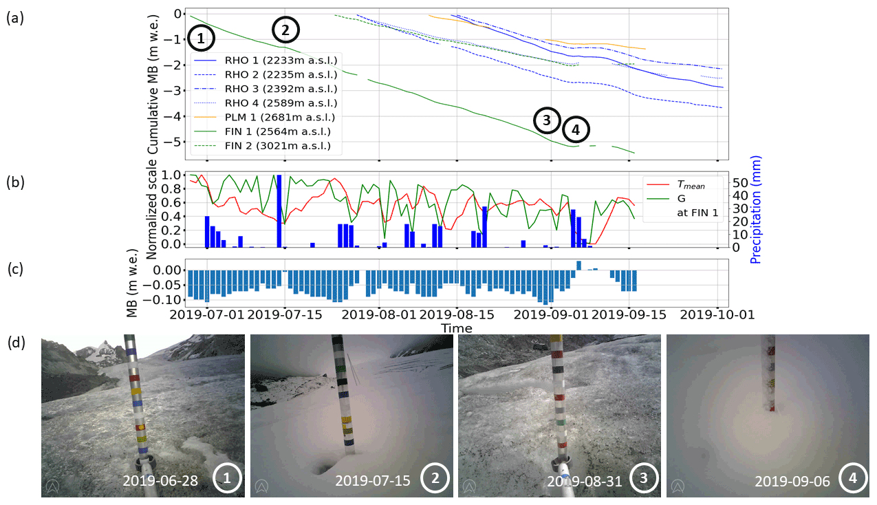
Figure 7 (a) Cumulative mass balance at individual camera stations during summer 2019. The circled numbers refer to the pictures shown in panel (d). (b) Normalized mean temperature T_mean and shortwave radiation G (left axis) normalized to their respective ranges, as well as precipitation (right axis) for station FIN 1. (c) Daily mass balance rate observed at FIN 1. (d) Sample images as captured by the camera at FIN 1: (1) camera right after setup, (2) glacier after light snowfall, (3) picture from the day with the highest melt (0.12 $\mathrm{m}\mathrm{w}.\mathrm{e}.$), and (4) snowfall event hampering the stake readout.

Considering all stations, we have observed ice melt rates of up to 0.12 $\mathrm{m}\mathrm{w}.\mathrm{e}.{\mathrm{d}}^{-\mathrm{1}}$ and a cumulative mass balance of about −5.5 $\mathrm{m}\mathrm{w}.\mathrm{e}.$ in 81 d close to the terminus of Findelgletscher (FIN 1). Different camera stations reveal different melt rates and total ablation, which generally depend on the station's elevation. However, stations at different elevations can have similar melt rates as well. For example, station RHO 4 at 2589 $\mathrm{m}\mathrm{a}.\mathrm{s}.\mathrm{l}.$ experienced an average melt rate of −0.047 $\mathrm{m}\mathrm{w}.\mathrm{e}.{\mathrm{d}}^{-\mathrm{1}}$, while the average melt rate at FIN 2 (3015 $\mathrm{m}\mathrm{a}.\mathrm{s}.\mathrm{l}.$) was −0.043 $\mathrm{m}\mathrm{w}.\mathrm{e}.{\mathrm{d}}^{-\mathrm{1}}$ during the same period (we count only days with net ablation). Further, station PLM 1 had the lowest average melt rate despite not being at the highest elevation. This might be due to the meteorological conditions, such as the formation of local cold air pools, and the so-called “Massenerhebung effect” (Barry, 1992). The latter describes the tendency of higher temperatures to occur at the same elevation in the inner Alps as on their outer margins. For all stations, average melt rates during July and August are similar (0.073 ± 0.012 $\mathrm{m}\mathrm{w}.\mathrm{e}.{\mathrm{d}}^{-\mathrm{1}}$ in July vs. 0.062 ± 0.011 $\mathrm{m}\mathrm{w}.\mathrm{e}.{\mathrm{d}}^{-\mathrm{1}}$ in August) and 0.02–0.03 $\mathrm{m}\mathrm{w}.\mathrm{e}.{\mathrm{d}}^{-\mathrm{1}}$ lower (i.e., 0.044 ± 0.014 $\mathrm{m}\mathrm{w}.\mathrm{e}.{\mathrm{d}}^{-\mathrm{1}}$) in September. On Glacier de la Plaine Morte, the difference is most pronounced with a drop of 0.06 $\mathrm{m}\mathrm{w}.\mathrm{e}.{\mathrm{d}}^{-\mathrm{1}}$ between August and September. Again, this is probably caused by local effects. On average, the difference between minimum and maximum melt measured at different stations on a particular day was 0.035 $\mathrm{m}\mathrm{w}.\mathrm{e}.{\mathrm{d}}^{-\mathrm{1}}$. Over the observational period, this difference ranged from 0.005 to 0.081 $\mathrm{m}\mathrm{w}.\mathrm{e}.{\mathrm{d}}^{-\mathrm{1}}$. The highest difference (0.081 $\mathrm{m}\mathrm{w}.\mathrm{e}.{\mathrm{d}}^{-\mathrm{1}}$) occurred on 1 September 2019 in connection with the passage of a convergence line and cold front (German Meteorological Service, 2019): while Glacier de la Plaine Morte was already under the influence of cooler weather, Findelgletscher and Rhonegletscher experienced another melt-intensive day. The variability at individual stations, measured as standard deviation of a 14 d running mean, was generally low during July and August (0.016 $\mathrm{m}\mathrm{w}.\mathrm{e}.{\mathrm{d}}^{-\mathrm{1}}$) and increased at the beginning of September (0.026 $\mathrm{m}\mathrm{w}.\mathrm{e}.{\mathrm{d}}^{-\mathrm{1}}$). We attribute this increase to the onset of intermittent snowfalls at individual sites.

As shown by the pictures from station FIN 1 (Fig. 7d), summer 2019 is characterized by a variety of events, ranging from very hot, melt-intensive days to snowfalls at high elevations. The time series of normalized mean daily temperature and shortwave radiation at station FIN 1 (Fig. 7b) illustrate that two heat waves occurred at the end of June and end of July 2019. The total amount of water released by snowmelt and ice melt on Swiss glaciers during these heat waves was 0.8 km³ (Swiss Academy of Sciences, 2019), which approximately equals the annual amount of drinking water consumed in the country. These extreme phases are also mirrored in the melt observed at our stations (Fig. 7): for FIN 1, daily melt rates peaked between 0.09 and 0.12 $\mathrm{m}\mathrm{w}.\mathrm{e}.{\mathrm{d}}^{-\mathrm{1}}$. For days with a range-normalized temperature exceeding 0.8 (9 d in total, Fig. 7b), the average melt rate is 0.1 $\mathrm{m}\mathrm{w}.\mathrm{e}.{\mathrm{d}}^{-\mathrm{1}}$ at that station. During these nine days, modeled, glacier-wide melt indicates the release of 6×10⁶ m³ of water. Another phase with very high melt occurred at the end of August 2019. Here, normalized temperature and radiation are average (mean values of 0.6 and 0.5, respectively). The exact causes for this strong melt event are unclear, and we speculate that it might be related (at least in part) to rain events that were not captured by the meteorological input despite being visible in our camera images between 28 and 31 August 2019. Summer melt phases were also interrupted by two snowfalls of different strengths: small amounts from 15 July 2019 (image 2 of Fig. 7d) and larger amounts, summing up to 0.25 m snow height in total, in early September (image 4 of Fig. 7).

4.2 Particle filter mass balance validation

Besides the direct observations presented above (Sect. 4.1), our framework enables predictions of daily mass balance. In this section, these predictions are (i) validated against reference forecasts (Sect. 4.2.1), (ii) cross-validated against test subsets of observations (Sect. 4.2.2), and (iii) compared against glacier-wide mass balances reported by GLAMOS (Sect. 4.2.3).

4.2.1 Validation against reference forecasts

We consider two types of reference forecasts: first, a forecast with (i) mean glacier-wide melt parameters as obtained from past calibration (Sect. 3.2) and (ii) the precipitation correction factor prcp_scale constrained by the 2019 GLAMOS winter mass balance; and second, a forecast with a partially informed model including the same constraint for prcp_scale but also a tuning of the melt parameters to reproduce one further intermediate point measurement. The latter measurement is the cumulative mass balance between September 2018 and 2019 at the mass balance stake closest to each camera (locations in Fig. 1). Since there are up to four stake readings per glacier, we calculate single parameter sets tuned to reproduce all possible combinations of stake readings per glacier. This results in 19 CRPS values in total, for which we calculate the median. We also distinguish between the case in which the uncertainties in the meteorological inputs are taken into account and the case in which they are not.

Finally, we calculate the CRPS for the two reference forecasts by inserting two different values into the CRPS equation: (a) the mass balance of each day separately and (b) the cumulative mass balance. Note that for the particle filter, there is no need to make this distinction. Indeed, the daily deviation from a mass balance observation also equals the deviation from the cumulative observation. Figure 8 shows the results of the validation.

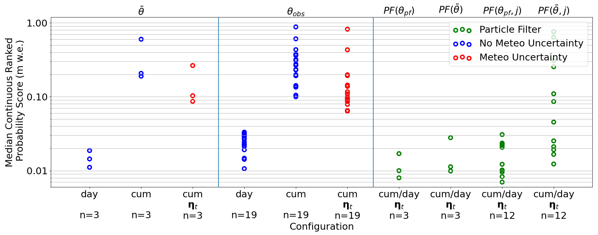
Figure 8 Median CRPS values over “n” validation cases for different forecasts. The following symbols are used: $\overline{\mathit{\theta }}$ = mean parameters from past calibration; θ_obs = parameters calibrated on different combinations of mass balance stake observations close to the cameras; θ_pf = parameters found with the particle filter. Cases accounting for (red dots and analyses with “η_t”) and neglecting (blue dots) the uncertainty in the meteorological variables are distinguished, and “cum” and “day” indicate the errors in the cumulative and daily mass balance predictions, respectively. For the particle filter (highlighted in green), the label “cum/day” indicates that the two errors coincide, and “j” indicates cases where the particle filter was run with only one model.

For the particle filter, daily and cumulative melt observations are generally reproduced well, with an average CRPS of 0.012 [0.012] m (proper CRPS outside and standard CRPS inside the square brackets). At the end of the assimilation period, Rhonegletscher has an average CRPS of 0.017 m, which is almost double the CRPS for Findelgletscher (CRPS = 0.01 m) and Glacier de la Plaine Morte (CRPS = 0.008 m). The high value of Rhonegletscher is related to the switch-on of cameras RHO 1 and RHO 3. Indeed, the glacier also has CRPS ≈ 0.01 m before that. Poor predictive performances also occur after snowfalls, probably related to the uncertainties by which the mass balance stake can be read during these times. We run experiments in which the particle filter is limited to using mean parameters and/or single models instead of parameter distributions and the model ensemble. In the experiments, the resulting average CRPS values are higher than the average CRPS obtained with the ensemble and time-variant parameters. The lowest single values occur for specific combinations when running the particle filter with the BraithwaiteModel and OerlemansModel and flexible parameters on Glacier de la Plaine Morte. Note that if no probabilistic temperature and precipitation lapse rate is used, the resulting CRPS values from the experiments with mean parameters and/or only one model are even higher than the highest CRPS obtained using the ensemble and time-variant parameters. The experiments thus show that it is beneficial to include all four models and parameter uncertainty into the particle filter.

Comparing the CRPS of the particle filter with the reference forecasts, the performance closest to the particle filter is delivered by the forecast produced with mean melt parameters and no uncertainty in the meteorological input (mean CRPS = 0.013 [0.015] m). When the CRPS is calculated from the cumulative mass balance produced with mean melt parameters, the CRPS increases to 0.333 [0.243] m on average. This is because the mean parameters do not adapt to the meteorological conditions over time, and in this case, the cumulative mass balance can temporarily be under- or overestimated or even diverge completely over time. Somewhat counterintuitively but for the same reason, the CRPS is similar when parameters have been tuned to match nearby stake readings. For the cumulative deviation, we find CRPS = 0.25 [0.251] $\mathrm{m}\mathrm{w}.\mathrm{e}.$ when considering meteorological uncertainty, and CRPS = 0.294 [0.28] $\mathrm{m}\mathrm{w}.\mathrm{e}.$ when not doing so. Compared to both the particle filter prediction and the prediction with mean melt parameters, the CRPS of daily mass balances produced without considering meteorological uncertainty is slightly higher (median CRPS: 0.023 [0.025] $\mathrm{m}\mathrm{w}.\mathrm{e}.$).

In general and for the individual glaciers, the particle filter improves the CRPS of the reference forecasts by 95 % to 96 %. For the daily forecasts, the performance of the particle filter is only partly better, with improvements in CRPS between 8 % and 48 %. Along with the performance, a further important advantage of the particle filter is that it provides daily estimates for the results' uncertainties without need for further calculations. Indeed, this information can be essential, especially for the operational application of our framework.

4.2.2 Cross-validation

A different approach for validating the particle filter is to only use subsets of the available camera observations as input and to evaluate the predicted mass balances at the remaining locations (cross-validation). We do so by splitting the available observations into training and test subsets of cameras, i.e., by keeping the time series of a given station together (as opposed to splitting individual time series). Our test sets always contains one time series; i.e., we perform a leave-one-out cross-validation. Figure 9 shows the temporal evolution of the CRPS at the test locations, i.e., at the stations not used by the particle filter.

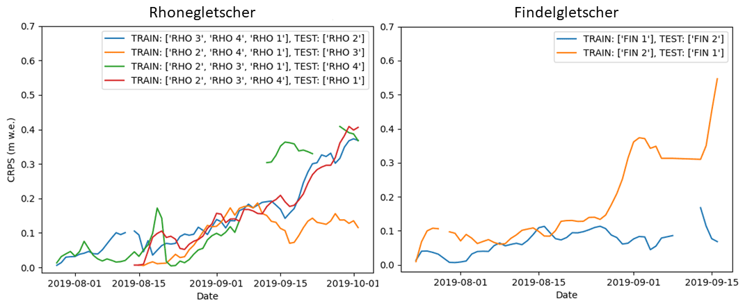
Figure 9 Temporal evolution of the CRPS as determined in a leave-one-out cross-validation procedure on Rhonegletscher and Findelgletscher. “TRAIN” and “TEST” stand for the stations assimilated by the particle filter and the station used for the validation, respectively.

We find that, in general, the cumulative mass balance at the test locations follows the cumulative observation curve well but not as closely as when the test location's data are assimilated with the particle filter. This shows the benefit of having several cameras per glacier mounted at different elevations. For Findelgletscher, we find 8.8 % average deviation (median CRPS of 0.071 and 0.108 $\mathrm{m}\mathrm{w}.\mathrm{e}.$ for the two stations) when comparing the cumulative mass balance curve with the particle filter prediction. For Rhonegletscher, the average deviation at the test locations is 9.0 % average deviation (median CRPS 0.14, 0.148, 0.067, and 0.178 $\mathrm{m}\mathrm{w}.\mathrm{e}.$ depending on the station). The highest CRPS values for Rhone stem from the period after the middle of August when two additional cameras were set up, but the values still outperform the reference forecasts of Sect. 4.2.1.

The temporal pattern evident in Fig. 9 includes an increasing CRPS through time but at different rates depending on the cross-validation subset. The individual pattern originates from (1) a stations' representativity for the given elevation band it is located in, (2) the combination of stations in the cross-validation subsets, and (3) cumulative error characteristics, since we observe cumulative mass balance over time. Station RHO 3, for example, can generally be modeled with lower errors compared to other stations. We speculate this being related to its location, which is in a relatively flat area with little crevasses. The other stations are instead either in the vicinity of crevasses (RHO 4) or influenced by shadows from the surrounding terrain, dark glacier surface, or steep ice (RHO 1 and RHO 2). RHO 1 and RHO 2 also show that even neighboring stations can exhibit different melt. This affects the results of the cross-validation whenever one of these two stations is excluded from the training dataset.

The above results show the ability of the particle filter to also predict melt at locations without observations, albeit with a lower performance when compared to the situation in which all observations are assimilated. The results also show that even with an augmented particle filter, it is demanding to find a unique, glacier-wide parameter set that correctly reproduces the mass balance at all locations.

4.2.3 Comparison to GLAMOS glacier-wide mass balances

We compare our assimilated model ensemble predictions to the glacier-wide annual mass balance reported by GLAMOS at the autumn field date of the mass budget year 2019. We do so by running the model from the field campaign date in autumn 2018. Figure 10 illustrates the different model and parameter settings used during the simulation.

Figure 10 Schematic model and parameter settings on Rhonegletscher during the mass budget year 2019. After an initial phase with parameters from past calibration, the precipitation correction factor prcp_scale is tuned to match the winter mass balance. When the first camera is set up, we sample the existing model runs 10 000 times to be able to couple the free model runs with the 10 000 particles during the particle filter period (not all are drawn for readability).

During the period preceding the installation of our cameras, we calculate mass balance with the parameters calibrated in Sect. 3.2. This results in about 45 distinct model runs, which we call “free model runs”. We use this first period to provide initial conditions for the particle filter period, which lasts from the first camera setup on a respective glacier either until cameras are retrieved or until the autumn field date is reached (whatever comes first). To achieve a connection between the free model run and the period during which the particle filter is used, we sample 10 000 times from the initial conditions at the first camera setup date. We refer to this procedure as “particle filtering without pre-selection (of initial conditions)”. Not all free model runs have to be used, though: they can also be pre-selected based on the cumulative mass balance observed at the stakes closest to the camera stations. For this case, we select model runs that reproduce these observations within an estimated reading uncertainty of ± 0.05 $\mathrm{m}\mathrm{w}.\mathrm{e}.$ (“particle filtering with pre-selection”). The cumulative mass balances calculated with these two procedures are compared to the GLAMOS analyses in Table 3.

Table 3 Mass balances calculated with the particle filter between the autumn field dates of 2018 and 2019 against the values reported by GLAMOS. See text for the difference of particle filtering with and without pre-selection. Uncertainty values are given as standard deviations.

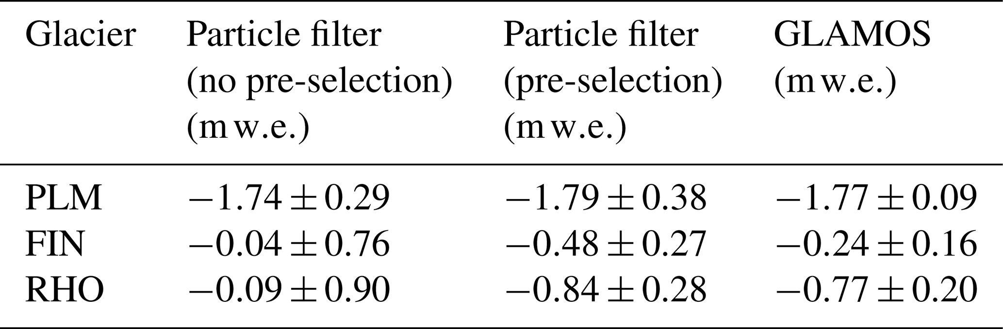
For particle filtering without pre-selection of initial conditions, the difference from the GLAMOS analyses is 0.67 $\mathrm{m}\mathrm{w}.\mathrm{e}.$ for Rhonegletscher, 0.2 $\mathrm{m}\mathrm{w}.\mathrm{e}.$ for Findelgletscher, and 0.05 $\mathrm{m}\mathrm{w}.\mathrm{e}.$ for Plaine Morte. With pre-selection, in contrast, the absolute difference changes by −0.07, −0.24, and +0.02 $\mathrm{m}\mathrm{w}.\mathrm{e}.$, respectively. Consequently, including the stake mass balance readings improves the match to the GLAMOS analyses for Rhonegletscher and Plaine Morte, while it has only little effect for Findelgletscher. A reason for this can be either that the mass balance stakes are not at the observation locations or that the mass balance gradients of the pre-selected runs are unfavorable. Overall, the differences from the GLAMOS analyses can be explained by (1) the difference in the approaches used to calculate glacier-wide mass balances from point observations, (2) the use of only 1–4 point observations located in the ablation zone and covering <30 % of the glacier elevation range, compared to the complete network of 5–14 stakes over the entire elevation range used in the GLAMOS analyses, (3) the lack of representativeness of the camera observations for the accumulation zone of the glaciers, i.e., biased vertical mass balance gradients, (4) the lack of representation of individual winter accumulation measurements in our glacier model, or (5) a problem with representing the mass balance of the glacier with only one parameter set. Also note that 91 %–99 % of the total uncertainty for the model runs with data assimilation stem from the period before the particle filter can be initialized, i.e., before the installation of the first camera station. Figure C1 in the Appendix shows the evolution of the mass balance state over the assimilation period by the example of Findelgletscher.

4.3 Individual model performance

We analyze model performance by considering the temporal evolution of the model probabilities π_t,j and model particle numbers N_t,j for the four melt models over time at individual glaciers. High model performance is indicated by high probabilities and large particle numbers over long time periods.

Figure 11 shows the model performance of all four melt models and at all three glaciers.

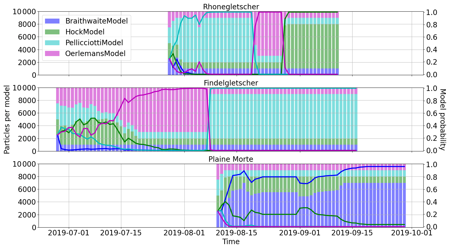
Figure 11 Temporal evolution of model probabilities (solid lines) and model particles (stacked bars) for the three modeled glaciers. The fast switch in model probabilities occurring for Findelgletscher between 07 and 8 August 2019 is further depicted in Fig. 12.

In general, we find that the model probabilities are sensitive to the ensemble input, such as the parameter priors, and the prescribed meteorological uncertainty. This is an indication of the ensemble choosing the model combination that best reproduces the observations at any time. Note that none of the models is removed from the ensemble in the resampling step even when the model performs poorly. During the assimilation period, indeed, models can recover and can show good performances at a later stage (see, for example, the HockModel for Rhonegletscher or the PellicciottiModel for Findelgletscher). This shows the utility of the resampling procedure introduced in Sect. 3.3.5.

During the assimilation period of an individual glacier, often one model dominates the ensemble for a given amount of time (“model dominance” being the case in which the model probability is >0.5). Model dominance, and especially fast switches between dominant models, can be indicative of a mode collapse, resulting from either an overconfident likelihood or prior, or both, operating in an M-open framework (Bernardo and Smith, 2009), i.e., the case in which the “true” model is not a choice amongst the available models. In our case, we believe that the ensemble prior might be overconfident on average since we have chosen the observational error conservatively; i.e., we have chosen the largest errors emerging in the round-robin experiment (Sect. 2.1.2). This would lead to a model preferably obtaining high weights, which had already dominated on the previous days. However, when the likelihood is overconfident or there is strong evidence that a previously well-performing model now performs worse, the filter might switch back and forth between individual models that best describe the observations. We accept this model dominance and the fast switching as a sign that the overall ensemble performance is improved. Averaged over all glacier and time steps, the PellicciottiModel has the highest model probability (0.39), while the BraithwaiteModel has an average model probability of 0.24, the OerlemansModel of 0.23, and the HockModel of 0.14. The relatively high probabilities assigned to the PellicciottiModel can have various reasons, and we suspect that two are of particular importance in our case: first, the calibration might have led to a broad prior parameter distribution, allowing for the model to adapt to various combinations of meteorological input and observed melt. Second, using the actual solar radiation G instead of the potential irradiation I_pot might provide a further advantage since this accounts for partly cloudy conditions and diffuse radiation, which the potential irradiation is not able to cover. The fact that the second highest probability is assigned to the OerlemansModel (which uses G as well), supports this possible explanation.

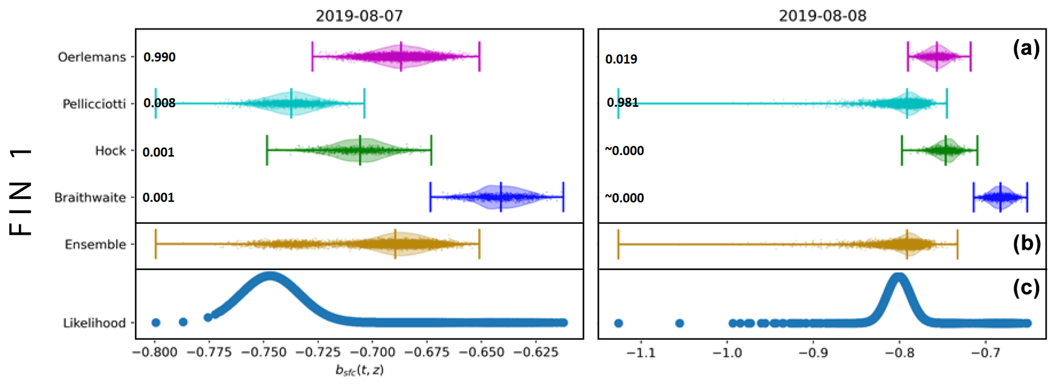
Figure 12 Violin plots with scattered particles as an example for a fast switch in assigned model probability (cf. Fig. 11). The example refers to Findelgletscher (station FIN 1). Shown are (a) predictions of the individual models, (b) the ensemble prediction, and (c) the particle likelihood for 2 subsequent days. The individual model probabilities are given to the right of the model names. Note that the ensemble is dominated by the OerlemansModel for the first day (left) and by the PellicciottiModel for the second day (right).

In terms of the temporal evolution, the model dominance for Rhonegletscher and Glacier de la Plaine Morte is determined already within the first few days and changes only a little after that. Changes in model dominance can be observed for Rhonegletscher and Findelgletscher, instead. In the case of Rhonegletscher, for example, the model dominance switches from the PellicciottiModel to the OerlemansModel and later to the HockModel. For Findelgletscher, however, there is a transition from the OerlemansModel to the PellicciottiModel. This transition is particularly noticeable between 7 and 8 August 2019 (Fig. 12). The causes for it are not entirely clear, and we speculate that it might be related to the precipitation event starting on 6 August. Perhaps surprisingly, the model dominance seems to be little influenced by snowfall events (e.g., from 9 to 17 September on Findelgletscher or from 5 September to 11 September on Rhonegletscher), even if surface albedo is taken into account very differently by the individual models.

Figure 13 shows the evolution of the distribution of individual model parameters during the assimilation period. The example refers to Findelgletscher.

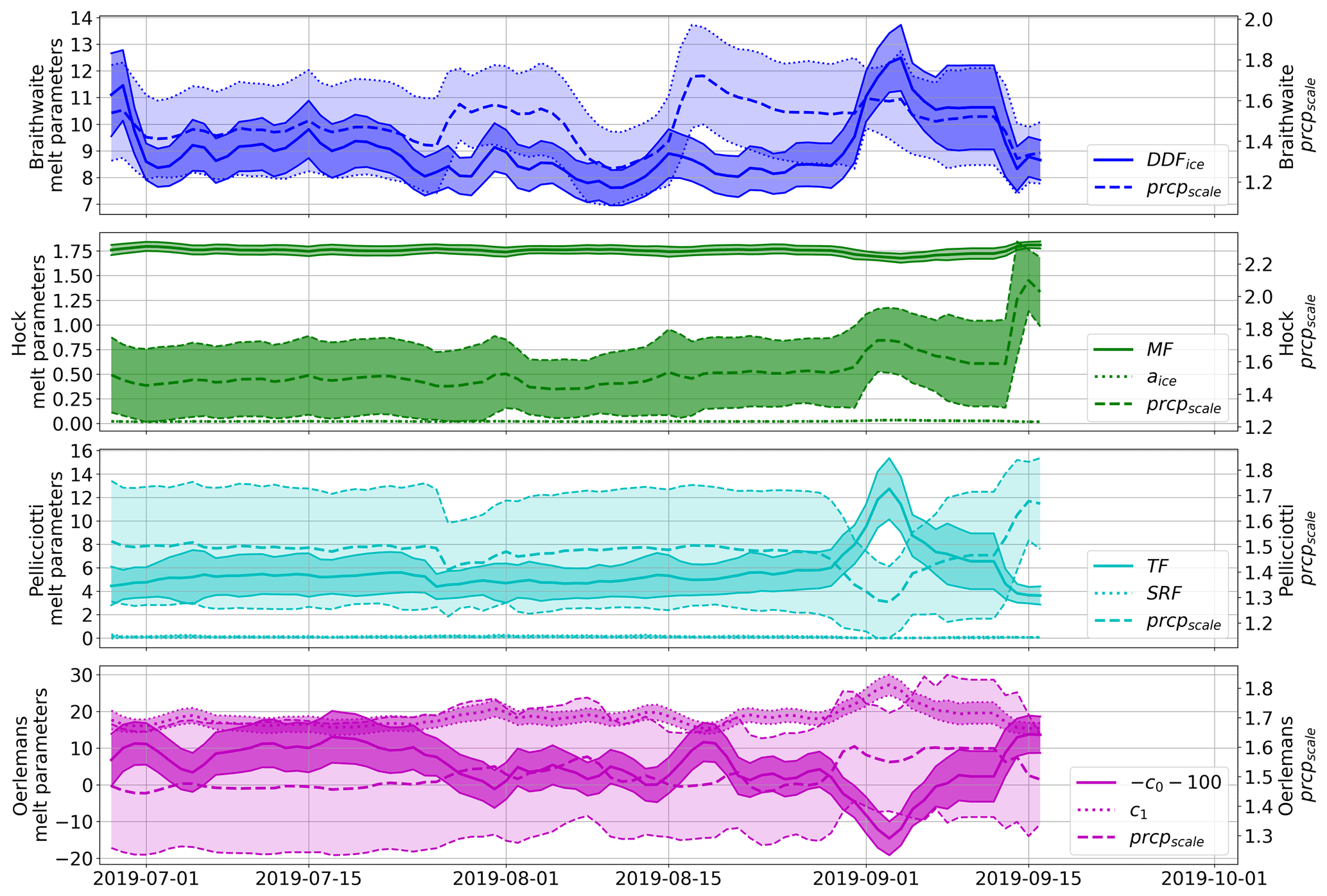
Figure 13 Temporal evolution of the various model parameters for Findelgletscher. Shown are the sample means (lines) and the standard deviations (bands). Note that for the OerlemansModel, parameter c₀ is adjusted to fit on the same scale as c₁.

Three phases of quick parameter changes can be observed. First, the parameters change rapidly on the first days of the assimilation period. This means that the prior parameter distributions do not match the exact parameter distributions needed to model the mass balance at the camera locations. This is due to both the calibration time span (seasonal calibration vs. daily application) and the low sample size of the calibrated parameters. A second rapid change can be observed after the second camera has been switched on, i.e., on 24 July 2019. Here, an adjustment in the parameters is needed in order to accommodate the mass balance at both stations equally well. The third rapid change starts when ablation at station FIN 1 is highest but when radiation and temperature are not at their maximum. Here, the change might be due to the model being forced to yield high ablation rates despite only moderate meteorological forcing. This shows the advantage of employing the model ensemble as opposed to, for example, a single model with deterministic parameters: the ensemble also reproduces system states which cannot be explained by the uncertain meteorological input.

5 Conclusions

In this study, we mounted seven cameras on three Swiss glaciers, delivering 352 point mass balance observations throughout summer 2019. At the camera locations, we observed daily melt rates of up to 0.12 $\mathrm{m}\mathrm{w}.\mathrm{e}.{\mathrm{d}}^{-\mathrm{1}}$ and cumulative melt of up to ∼5 $\mathrm{m}\mathrm{w}.\mathrm{e}.$ in 81 d. To calculate near-real-time mass balances, we used an ensemble of three TI models, a simplified energy balance model, and meteorological model input. The camera observations were assimilated into the model ensemble by using a specifically developed particle filtering scheme. The particular focus was put on delivering a stable ensemble capable of reproducing glacier mass balance throughout the summer. Variability in the model parameters, as well as particle filter stability, was considered. For the former, a prior parameter distribution obtained from calibration against past seasonal glaciological mass balances was used as input to an augmented particle filter capable of estimating parameters while assimilating observations. For the latter, the particle filter was designed such that models with temporarily poor performance can recover at a later stage. For the mass budget year 2019, we calculate cumulative mass balances of −1.79 $\mathrm{m}\mathrm{w}.\mathrm{e}.$, −0.48 $\mathrm{m}\mathrm{w}.\mathrm{e}.$, and −0.84 $\mathrm{m}\mathrm{w}.\mathrm{e}.$ for Glacier de la Plaine Morte, Findelgletscher, and Rhonegletscher, respectively.

The mass balances given by the particle filter were closer to the cumulative observations (CRPS = 0.012 $\mathrm{m}\mathrm{w}.\mathrm{e}.$) than two reference forecasts which either assumed no measurements to be available or only used one intermediate set of stake readings. Measured with the CRPS for cumulative mass balances, the particle filter improves the performance of reference forecasts by 95 % to 96 %. As a further advantage, the particle filter delivers direct uncertainty estimates. A leave-one-out cross-validation procedure showed that the cumulative mass balance predicted with the particle filter is within 9 % of the observations at any location. In an analysis of the individual model performance, we found that our technique to prevent models from being removed from the ensemble is useful since models can recover at a later stage. In terms of model ensemble, the TI model by Pellicciotti et al. (2005) obtained the highest average model probability (0.39). None of the four models has an average probability <10 %, and even if individual models can temporarily perform poorly, our technique preventing models from being removed from the ensemble completely allows them to recover at a later stage. Fast temporal switches between model probabilities are attributed to overconfident likelihood or prior distributions, or both. As a future venture, we envision an extension of the particle filter in which glacier mass balances and model parameters are further constrained by remotely sensed observations of albedo and snow lines. These measurements are indirect but have the potential to (1) complement the camera observations extensively and to (2) overcome the limited knowledge about the spatial and temporal extrapolation of glacier mass balances and model parameters.

Appendix A: Handling of multiple cameras

Assume that camera i is installed at elevation z_i on day t_i−1, where $t_{\mathrm{0}}<t_{\mathrm{1}}<t_{\mathrm{2}}\mathrm{\dots }$ (to be coherent with earlier notation that the first camera is installed at time t₀). From time t_i−1 onwards, we include $b_{\mathrm{sfc}}(t_{i-\mathrm{1}},z_i)$ in the state vector as a component which remains constant. Then the observations at time $t>t_{i-\mathrm{1}}$ are functions of the state at time t:

$$\begin{array}{}\text{(A1)}& h(t,z_i)={\displaystyle \frac{b_{\mathrm{sfc}}(t,z_i)-b_{\mathrm{sfc}}(t_{i-\mathrm{1}},z_i)}{{\mathit{\rho }}_{\mathrm{bulk}}}}+\mathit{ϵ}(t,z_i).\end{array}$$

The true value of $b_{\mathrm{sfc}}(t_{i-\mathrm{1}},z_i)$ is unknown, and the uncertainty is represented by the values $b_{\mathrm{sfc},k}(t_{i-\mathrm{1}},z_i)$ of the particles. Thus at time t, the contribution from the observation h(t,z_i) to the weight of particle k is proportional to

$$\begin{array}{}\text{(A2)}& \exp \left(-{\displaystyle \frac{\left(h\right(t,z_i)-(b_{\mathrm{sfc},k}(t,z_i)-b_{\mathrm{sfc},k}(t_{i-\mathrm{1}},z_i))/{\mathit{\rho }}_{\mathrm{bulk}}\cdot {\mathit{\rho }}_{\mathrm{w}}{)}^{\mathrm{2}}}{\mathrm{2}{\mathit{\sigma }}_{\mathit{ϵ}}^{\mathrm{2}}}}\right).\end{array}$$

Although $b_{\mathrm{sfc},k}(t_{i-\mathrm{1}},z_i)$ never changes during the propagation step, it will change in the resampling steps. Thus the uncertainty about $b_{\mathrm{sfc}}(t_{i-\mathrm{1}},z_i)$ will decrease as time proceeds. This is presumably not realistic, but the effect of small errors in the baseline also diminishes as time proceeds.

Appendix B: Resampling procedure

The technical details of the resampling procedure in Sect. 3.3.5 are the following: if, after prediction and update, N_t,j denotes the number of particles with model index j, we prevent models from not being resampled by choosing a minimum model contribution $\mathit{\varphi }<\frac{\mathrm{1}}{\mathrm{4}}$ to the ensemble. This ensures that the resampling step preserves a minimum particle number $N_{t,j}\ge \mathit{\varphi }{N}_{\mathrm{tot}}$ representing model j. For our application, we choose ϕ=0.1. If the posterior probability of model j (Eq. 21) is smaller than the minimum contribution ϕ, an unweighted sample that represents π_t,j correctly must have less than ϕN_tot particles with model index j. To ensure our minimum contribution condition though, we generate a weighted sample $({\stackrel{\mathrm{̃}}{\mathit{x}}}_{t,k},{\stackrel{\mathrm{̃}}{w}}_{t,k})$ such that each model index j appears at least ϕN_tot times, and the weights are as close to uniform as possible. We select the particles ${\stackrel{\mathrm{̃}}{\mathit{x}}}_{t,k}$ in a two-step resampling procedure: first, the number N_t,j of particles with model index j is chosen to be $N_{t,j}=\mathit{\varphi }{N}_{\mathrm{tot}}+L_{t,j}$, where L_t,j are excess frequencies. We obtain these frequencies by sampling a total of N_tot(1−4ϕ) model indices from $\mathit{\{}\mathrm{1},\mathrm{2},\mathrm{3},\mathrm{4}\mathit{\}}$ with weights proportional to how much a model probability exceeds the chosen minimum contribution, i.e., $max(\mathrm{0},{\mathit{\pi }}_{t,j}-\mathit{\varphi })$. In a second step, we draw for each model a resample of size N_t,j with weights $w_{t,k}/{\mathit{\pi }}_{t,j}$ from the particles with model index j. The combined set of the N_tot resampled particles gives the new filter particles ${\stackrel{\mathrm{̃}}{\mathit{x}}}_{t,k}$.

However, introducing a restriction on the minimum number of particles per model can lead to biased estimates as poor models with probability ${\mathit{\pi }}_{t,j}\le \mathit{\varphi }$ are overrepresented in the ensemble. To compensate for poor models occurring too often among the resampled particles (and the other models not often enough), the following weight has to be given to ${\stackrel{\mathrm{̃}}{\mathit{x}}}_{t,k}$:

$$\begin{array}{}\text{(B1)}& {\stackrel{\mathrm{̃}}{w}}_{t,k}={\displaystyle \frac{{\mathit{\pi }}_{t,j}}{N_{t,j}}}\text{ if }{\stackrel{\mathrm{̃}}{m}}_{t,k}=j.\end{array}$$

These weights sum to unity and preserve the original weights w_t,k on average. Since they can become very small though, we work with the logarithm of the weights to avoid numerical underflow. It should be noted that we insert ${\stackrel{\mathrm{̃}}{w}}_{t-\mathrm{1},k}$ for $w_{t-\mathrm{1},k}$ in Eqs. (14) and (20). In order to see that the weights we choose for ${\stackrel{\mathrm{̃}}{\mathit{x}}}_{t,k}$ are correct, we denote the number of times the particle x_t,k is selected in the resampling procedure by ${\stackrel{\mathrm{̃}}{M}}_{t,k}$. This means that the resampling gives x_t,k the random weight $\frac{{\stackrel{\mathrm{̃}}{M}}_{t,k}}{N_{\mathrm{tot}}}$, which is then multiplied by the additional weight ${\stackrel{\mathrm{̃}}{w}}_{t,k}$. Hence, x_t,k receives the total weight

$$\begin{array}{}\text{(B2)}& w_{t,k}^{\prime }={\stackrel{\mathrm{̃}}{w}}_{t,k}{\displaystyle \frac{{\stackrel{\mathrm{̃}}{M}}_{t,k}}{N_{\mathrm{tot}}}}.\end{array}$$

If $m_{t,k}=j$, it holds that

$$\begin{array}{}\text{(B3)}& \begin{array}{rl}E(w_{t,k}^{\prime }\mid N_{t,j})& ={\stackrel{\mathrm{̃}}{w}}_{t,k}E({\stackrel{\mathrm{̃}}{M}}_{t,k}/N_{\mathrm{tot}}\mid N_{t,j})\\ & ={\displaystyle \frac{{\mathit{\pi }}_{t,j}}{N_{t,j}}}{\displaystyle \frac{w_{t,k}{N}_{t,j}}{{\mathit{\pi }}_{t,j}}}=w_{t,k},\end{array}\end{array}$$

i.e., on average the new weights $w_{t,k}^{\prime }$ are equal to the original weights.

Appendix C: Temporal evolution of the mass balance state with the example of Findelgletscher

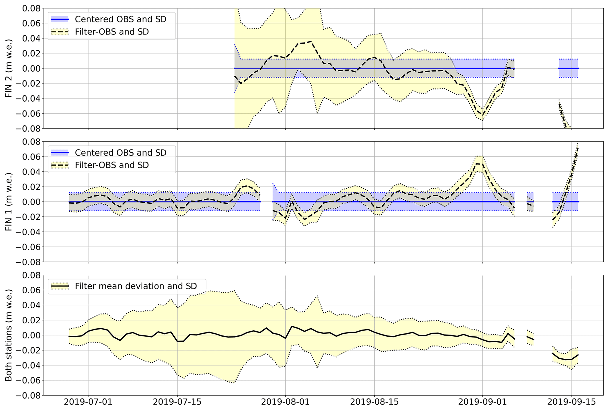
Figure C1 Temporal evolution of the ensemble mass balance state at stations FIN 1 and FIN 2. In the top two panels, the evolution of the mean and standard deviation of the filter (black lines and yellow shaded area) around the centered observations (blue lines and blue shaded area) is shown. In the bottom panel the mean deviation of the filter from the observations at both stations is shown.