the Creative Commons Attribution 4.0 License.
the Creative Commons Attribution 4.0 License.
 | 04 Oct 2021
High-resolution inventory to capture glacier disintegration in the Austrian Silvretta
Andrea Fischer
Gabriele Schwaizer
Bernd Seiser
Kay Helfricht
Martin Stocker-Waldhuber
A new high-resolution glacier inventory captures the rapid decay of the glaciers in the Austrian Silvretta for the years 2017 and 2018. Identifying the glacier outlines offers a wide range of possible interpretations of glaciers that have evolved into small and now totally debris-covered cryogenic structures. In previous inventories, a high proportion of active bare ice allowed a clear delineation of the glacier margins even by optical imagery. In contrast, in the current state of the glacier only the patterns and amounts of volume change allow us to estimate the area of the buried glacier remnants. We mapped the glacier outlines manually based on lidar elevation models and patterns of volume change at 1 to 0.5 m spatial resolution. The vertical accuracy of the digital elevation models (DEMs) generated from six to eight lidar points per square metre is of the order of centimetres. Between 2004/2006 and 2017/2018, the 46 glaciers of the Austrian Silvretta lost −29 ± 4 % of their area and now cover 13.1 ± 0.4 km2. This is only 32 ± 2 % of their Little Ice Age (LIA) extent of 40.9 ± 4.1 km2. The area change rate increased from 0.6 %/yr (1969–2002) to −2.4 %/yr (2004/2006–2017/2018). The Sentinel-2-based glacier inventory of 2018 deviates by just 1 % of the area. The annual geodetic mass balance referring to the area at the beginning of the period showed a loss increasing from −0.2 ± 0.1 m w.e./yr (1969–2002) to −0.8 ± 0.1 m w.e./yr (2004/2006–2017/2018) with an interim peak in 2002–2004/2006 of −1.5 ± 0.7 m w.e./yr. To keep track of the buried ice and its fate and to distinguish increasing debris cover from ice loss, we recommend inventory repeat frequencies of 3 to 5 years and surface elevation data with a spatial resolution of 1 m.
- Article
(38477 KB) - Full-text XML
-
Supplement
(2667 KB) - BibTeX
- EndNote


As a reaction to climate change, mountain glaciers all over the world are changing at an increasing pace (IPCC, 2019) and at unprecedented rates (Zemp et al., 2015) but with significant regional variability (IPCC, 2019). It is widely accepted that in some mountain ranges a significant part of today's glaciers may disappear within this century (e.g. Zemp et al., 2019a; Huss and Fischer, 2016). A loss of almost all mountain glaciers by 2300 seems possible (Marzeion et al., 2012). For assessing climate change using glaciers as essential climate variables (Bojinski et al., 2014), the precise and detailed monitoring of glacier recession is essential (Zemp et al., 2019b). It can also reveal regionally different response times (Zekollari et al., 2020) and various uncertainties (Huss et al., 2014) and serve as a basis for specific scenarios (e.g. Zekollari et al., 2019).
Glacier inventories are amongst the most valuable tools for glacier monitoring on a regional scale (Haeberli et al., 2007; Gärtner-Roer et al., 2019) and for remote and large glaciers. After the pioneering World Glacier Inventory (WGI), compiled by WGMS and NSIDC (1999), several initiatives, such as GLIMS (Kargel et al., 2014; Racoviteanu et al., 2009), have published global glacier inventories like the Randolph glacier inventory (Pfeffer et al., 2014). International consortia like GlobGlacier work out guidelines for mapping glaciers (e.g. Paul et al. 2009). At the same time, smaller regional studies work on new methods (e.g. Paul et al., 2020) and have responded to regional phenomena and demands, for example mapping of debris-covered glaciers (Nagai et al., 2016) or the large and often cloudy and snow-covered Patagonian glaciers (Meier et al., 2018). Regional inventories at high resolution can also serve as validation for large-scale semi-automatic remote-sensing products.
Airborne lidar has been a valuable tool for glacier studies for nearly 20 years (e.g. Geist and Stötter, 2002; Pellikka and Rees, 2009). Acquisition technologies, processing, and analysis have been significantly improved since the early years and now reach a few centimetres nominal vertical accuracy in flat areas. High point densities allow gridded elevation data to be processed with a spatial resolution of 0.5 m or even higher. Early scientific work included investigating the potential of (repeat) lidar data to map geomorphological processes (Höfle and Rutzinger, 2011) and glacier/rock glacier extent (Abermann et al., 2010). From 2004 onwards, federal authorities in Austria initiated the compilation of the first federal digital elevation models (DEMs) based on lidar, which were used to update the photogrammetric Austrian glacier inventories (Fischer et al., 2015a, b). Now a repeat federal lidar DEM is available for several regions in Austria, like the Silvretta range where the DEM Vorarlberg dates from 2017 and the DEM of the Tyrolean Silvretta from 2018 (black polygon in Fig. 1).
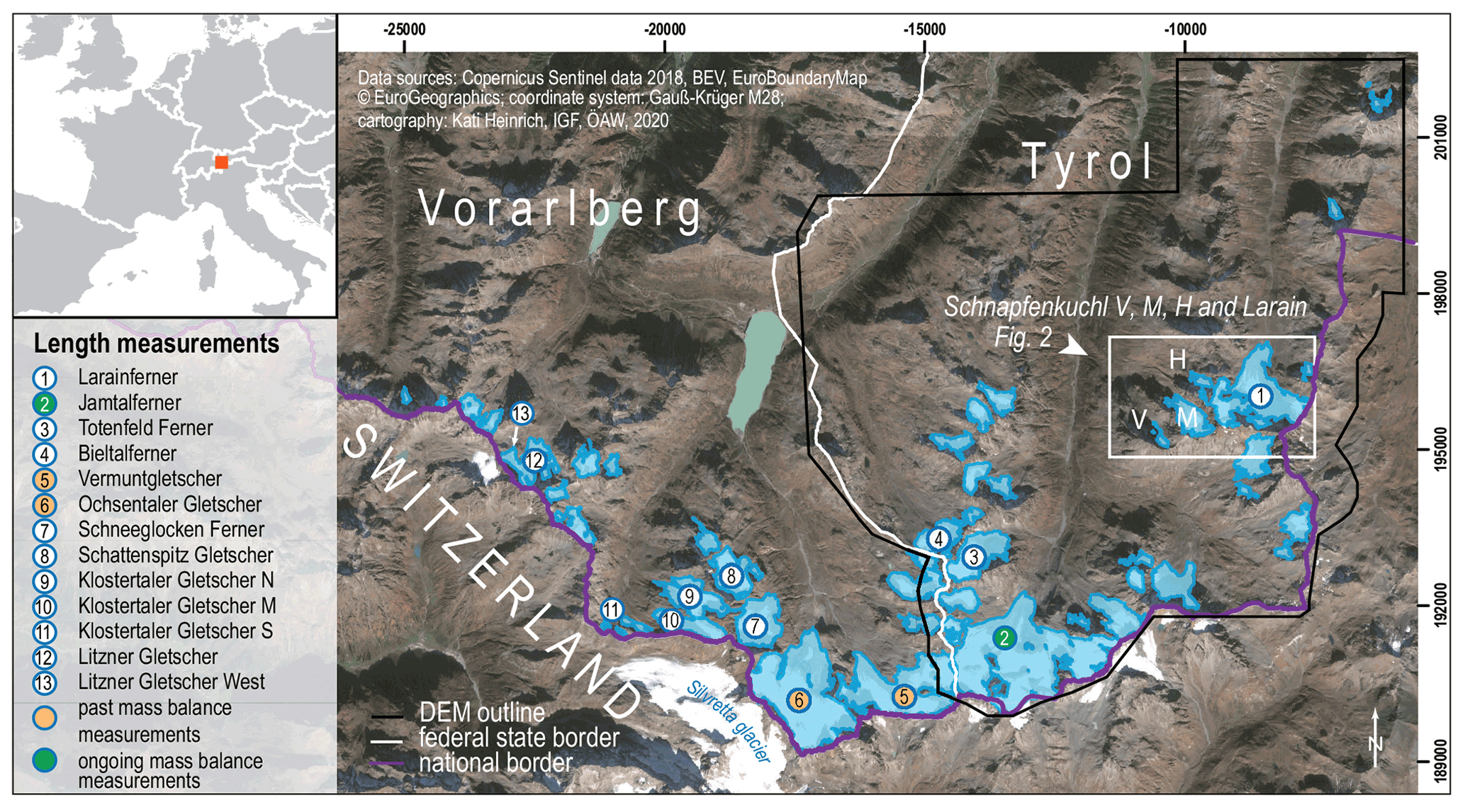
Figure 1Overview of the glaciers and ongoing and past mass balance and fluctuation time series in the Austrian part of the Silvretta range. The DEM of the Tyrolean part dates from 2018 (black outline) and of Vorarlberg from 2017.
In this article, we present a new lidar-based glacier inventory and the respective geodetic mass balance of the Austrian Silvretta (Fig. 1), located in the federal states of Tyrol and Vorarlberg. This inventory presents the glacier area and surface elevation for the years 2017 (Vorarlberg) and 2018 (Tyrol). Here, for the first time, a regional glacier inventory was derived from two high-resolution lidar surveys for a period of the beginning of glacier down waste indicated by the extreme melt during the summer of 2003. Repeated lidar has the potential to map volume loss caused by the melt of debris-covered ice (Abermann et al., 2009). The mass balance monitoring at Jamtalferner glacier indicates extremely negative mass balances since 2003 (Fischer et al., 2016c) in all elevation zones. As a result, the glacier darkens and disintegrates so that the delineation of glacier outlines becomes increasingly uncertain if based on visible imagery only. The evolution of the other glaciers in the region is similar, making it useful to include the derived volume changes in the analysis to delineate the debris-covered glacier margins. The volume change was also used to estimate the geodetic mass balance of the 46 glaciers for the period 2004/2006–2017/2018 with two different reference areas: the area at the beginning of the period and the average area.
Large and continuous mass losses resulted in significant changes in glacier geomorphology and topography in the Austrian Silvretta. For example, in recent years the Schnapfenkuchl V and H glaciers (Figs. 2 and 3 and close-ups in Figs. S1 and 4) cannot at first glance be identified even during a field survey as bare ice is rarely visible. The geomorphological structure of the totally debris-covered surface is not dominated by ice dynamics, with crevasses, steep lateral moraines causing different inclinations of glacier areas and adjacent surfaces, or depressions at the ice margins, as could be expected for larger debris-covered valley glaciers.
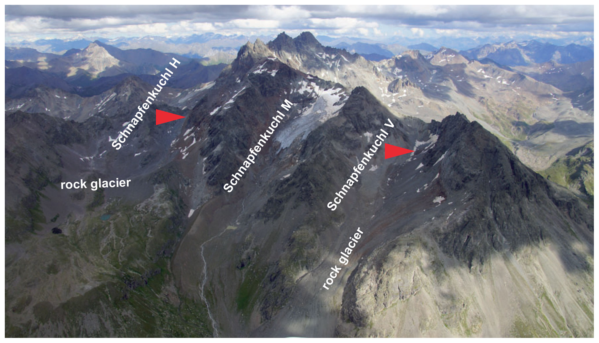
Figure 2Aerial overview of the Schnapfenkuchl glaciers V, M, and H in an aerial photograph of 21 August 2020 (photograph by Andrea Fischer). While Schnapfenkuchl M still is a classic glacier with exposed bare ice, on Schnapfenkuchl H and V bare ice is rarely exposed. See the close-ups of the parts with ice exposed (red arrows) in Fig. S2.
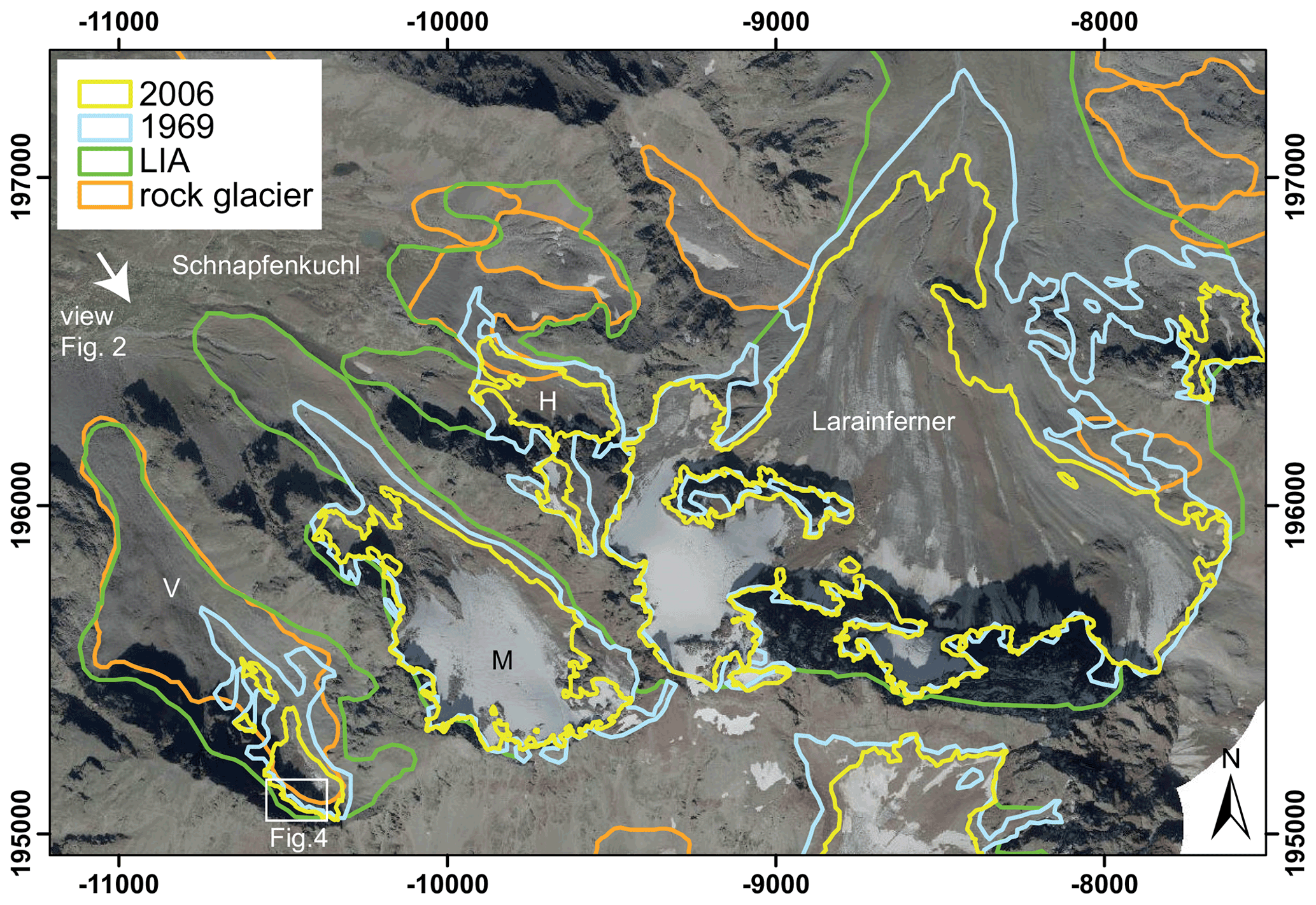
Figure 3Overview of the Schnapfenkuchl glaciers V, M, and H in an orthophoto of 2020 with the information available prior to the new glacier inventory: the glacier margins of the former glacier inventories for LIA, 1969, and 2006 and rock glacier margins (Krainer and Ribis, 2012). While the ice margin of Schnapfenkuchl M and Larainferner is clearly visible, the delineation of Schnapfenkuchl V and H glaciers from the orthophoto can only be guessed at.
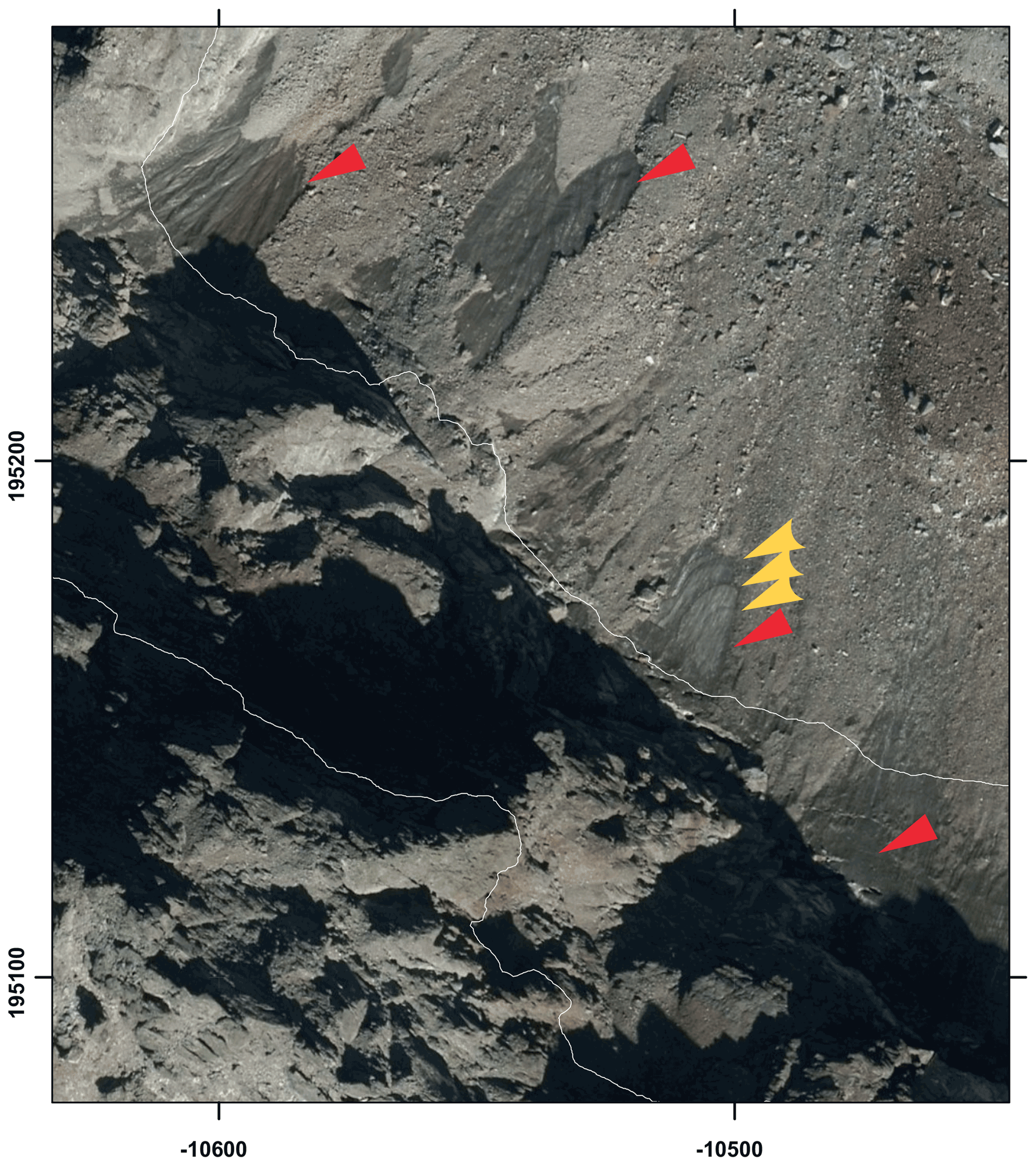
Figure 4Bare ice exposed (red arrows) at Schnapfenkuchl glacier V in an orthophoto from 2015 (red arrows), with stratigraphic layers (yellow arrows) indicating sedimentary ice or firn. Orthophotos: CC 4.0 https://www.data.gv.at/katalog/en/dataset/orthofoto (last access: 23 September 2021).
Schnapfenkuchl V and H glaciers were clearly identified as glaciers in past inventories: they showed exposed bare ice, accumulation areas, and an englacial drainage system, and crevasses as indicators for ice dynamics were present. In recent years, traditional and evident properties of a glacier became hidden by debris (see Fig. 5 for the evolution of Schnapfenkuchl H glacier). In the orthophotos of 1954, 1970, and 2002, Schnapfenkuchl H glacier can be clearly identified as a glacier, while in 2009, 2015, and 2020 we would hardly map Schnapfenkuchl V and H as glaciers when compiling the first glacier inventory of the region due to the debris cover (Fig. S2a–c).
The increasing debris cover is not restricted to the few small glaciers like Schnapfenkuchl H and V. It is a widespread phenomenon in the Austrian Silvretta, also evident from regular field surveys. For example, length change measurements at one of the largest glaciers of Austrian Silvretta, Litzner glacier (Fig. 1), were abandoned because the identification of the glacier margin was hampered by the increasing debris cover at the glacier tongue. Figure S3 illustrates that the glacier tongue was totally covered by debris within only about a decade: in 2006, bare ice at the tongue is clearly evident in the orthophoto but not in 2012 and 2015. Moreover, the higher glaciers, like Verhupf glacier, are affected in a way which potentially impacts on the accuracy of glacier delineation. The small glaciers which remained fairly unchanged in the last inventories (Abermann et al., 2009) were affected in a way which is relevant for compiling glacier inventories: the formerly ice-covered and now exposed steep rock faces release rock and debris onto the glacier surface. Melt rates of more than 1 m w.e./yr recorded at the Jamtalferner even at elevations above 3000 m (Fischer et al., 2016c) were recorded after 2003, removing the firn layers and decreasing albedo. The ice thickness at higher elevations is often smaller than at the glacier tongue for which an annual melt rate of 1 m could correspond to 5 % of the total thickness (e.g. Fischer and Kuhn, 2013), exposing rock outcrops of a rough bed topography. One example of this process is the evolution of Schnapfenkuchl H glacier illustrated by a time series of orthophotos (Fig. 5).
Many glaciers in the Austrian Silvretta were reported to switch from the moderate glacier retreat of the last 150 years to a rapid down waste close to a fade out of the ice (Fischer et al., 2016a, b, c, example in Fig. 5). As these processes are related to the rapid recession of mountain glaciers, which have potentially occurred not only in the Austrian Silvretta during the last decade but sooner or later will in other mountain regions also, we have to validate and elaborate our monitoring strategies to capture this process. This is important on a local and global level as small glaciers not only contribute to sea level rise (Bahr and Radić, 2012) but can also be important for local hydrological and hazard management. The precise monitoring of the transition to a glacier-free landscape is also important for the interpretation and dating of palaeo-glacial landforms, as studied in the Austrian Silvretta by Braumann et al. (2020).
The now very small and rapidly down-wasting glaciers of the Austrian Silvretta are perfect for testing and analysing the potentials and limitations of repeat lidar as a high-resolution airborne remote-sensing method for monitoring glacier fade out in qualitative and quantitative terms.
By definition, the new glacier inventory can be used to estimate the changes in area and volume of all glaciers in a specific region. This raises the following research questions: which of the potentially transient cryogenic structures (e.g. Fig. 5, year 2020) should remain part of a glacier inventory, and what is the possible effect of neglecting ice remnants in the inventory?
To answer the research questions related to the compilation of glacier inventories in a stage of early deglaciation, this study presents
- i
a new glacier inventory based on two high-resolution lidar DEMs to identify and quantify glacier areas in 2017/2018;
- ii.
the rate of area and volume changes since the last glacier inventories of 1850, 1969, 2002, and 2004/2006;
- iii.
a discussion of the potential and limitations of repeat lidar to map glacier changes under current glacier states;
- iv.
a discussion of glacier inventory strategies to monitor transient glacier states under conditions of rapid glacier decay close to complete loss of ice.
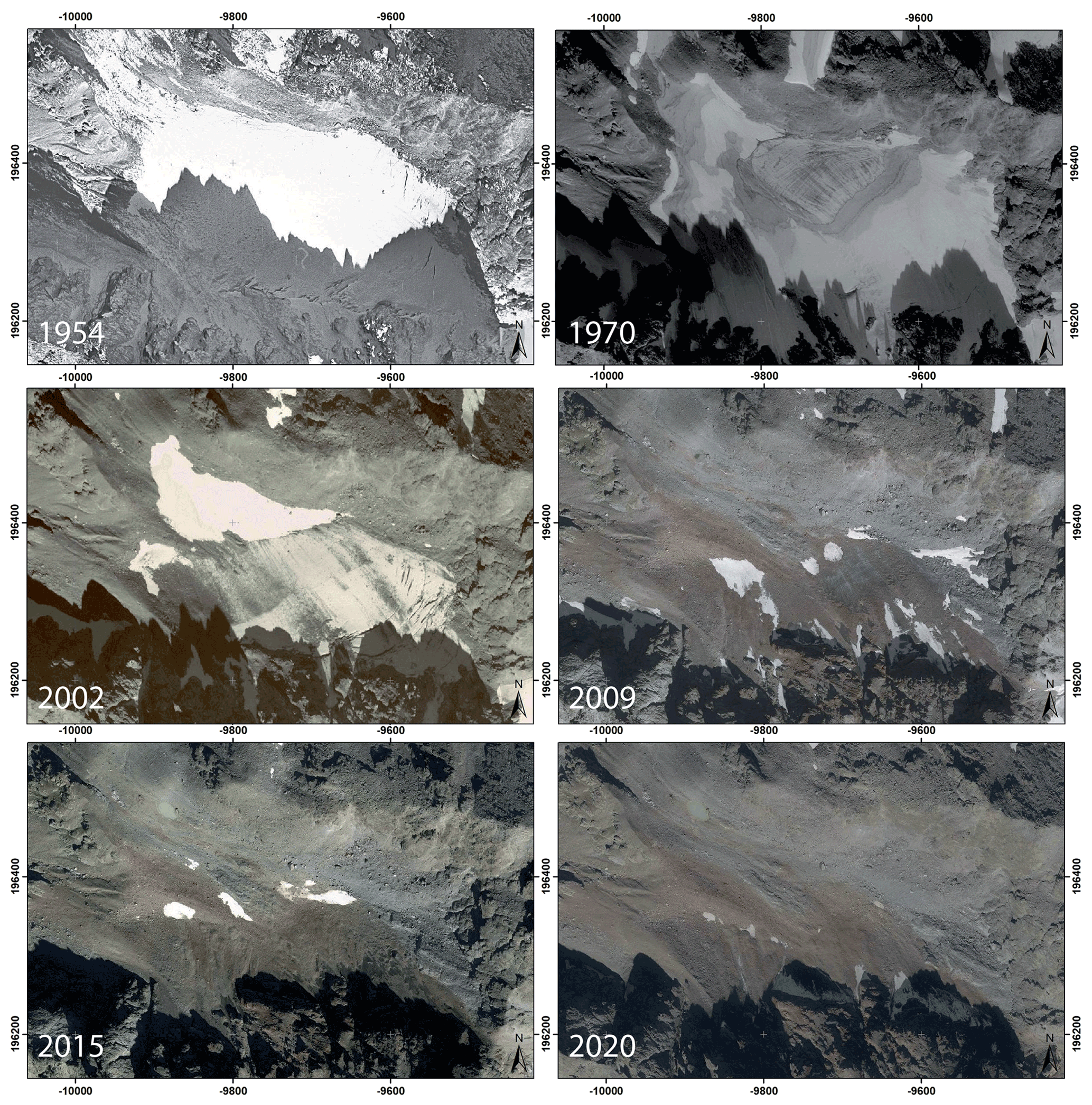
Figure 5The evolution of Schnapfenkuchl glacier V in a time series of orthophotos from 1954 to 2020 illustrates that the evolution from a glacier with crevasses as visible indicators of ice dynamics took just 20 years. In the orthophotos of 2009 and 2015, bare ice is still visible at the surface. Orthophotos: CC 4.0 https://www.data.gv.at/katalog/en/dataset/orthofoto.
2.1 Orthophotos 2015/2018 and surface elevations for 2017/2018
Surface elevation data for 2017/2018 were made available by the federal administrations of the provinces of Tyrol and Vorarlberg (see the locations of the glaciers in Fig. 1). The orthophotos of Tyrol date from summer 2015 for the southern part and from 2018 for the northern part (data.tirol.gv.at, 2021). The orthophotos of Vorarlberg date from 2018 and are available via the WMS Service geoland.at (2021). The spatial resolution of the images is 0.2–0.5 m.
The airborne lidar digital elevation models used for mapping glaciers in this study date from 2017 (Vorarlberg) and 2018 (Tyrol) with horizontal resolutions of 0.5×0.5 m (Vorarlberg) and 1×1 m (Tyrol).
The lidar DEMs of 2017 and 2018 were both coregistered to the national GIS grid with elevation (BEV, 2011) as a national standard procedure. The coregistration of the high-resolution full waveform lidar DEMs to the earlier lidar DEMs with lower spatial resolution is not considered the state of the art of lidar technology (Maria Attwenger, personal communication) as modern processing techniques refer to point clouds and reference areas to ensure the accuracy of the represented surface topography.
For the lidar data of Vorarlberg, the Silvretta was covered by 76 flight stripes during 14 and 29 August 2017. Quality control was carried out with ORIENT-LIDAR, resulting in a σ0 of 0.028 m and an RMS for control area residuals of 0.004/0.004/0.016 m in and 0.056/0.056/0.031 m for all points (Würländer, 2019). In the final report for the Tyrolean part (Rieger, 2019) the uncertainty estimate of the lidar data processed with the OPALS software is estimated by the comparison to control areas. The resulting standard deviation of elevation at the control areas is 0.032 m. The control area located in the subsample we used for the study showed a standard deviation of 0.030 m. All control areas are located on stable ground outside glaciers.
2.2 Areas and surface elevations in previous glacier inventories
For the Austrian part of the Silvretta range, we compiled glacier area (A) changes relative to the Little Ice Age (LIA) maximum from mapping moraines for 1969, 1996, and 2002 from orthophotos and for 2004 (Vorarlberg) and 2006 (Tyrol) from existing glacier inventories (Fischer et al., 2015a, b). For all inventories apart from the LIA inventory, not only glacier areas but also glacier surface elevations are available. The glacier margins were delineated manually with an uncertainty of the resulting area (σA) of ±1.5 % for glaciers larger than 1 km2 and ±5 % for smaller ones (Abermann et al., 2009).
The uncertainty of surface elevations of glaciers as quantified by Abermann et al. (2010) is less ±0.3 m for the DEMs based on the lidar flights in 2004 and 2006. The federal administration of Tyrol quantifies the single point standard deviation as 0.03 m based on the analysis of pass areas (Federal Government of Tyrol, 2020). The federal administration of Vorarlberg evaluated their DEM of 2004 with 58 597 object elevations and 49 483 terrestrially measured points of different types and found a mean elevation difference of −0.04 and −0.05 m respectively. A total of 95 % of the points meet an accuracy of ±0.4 m (Landesvermessungsamt Feldkirch, 2004).
2.3 Comparison of nominal relative uncertainties of all lidar data used in the study
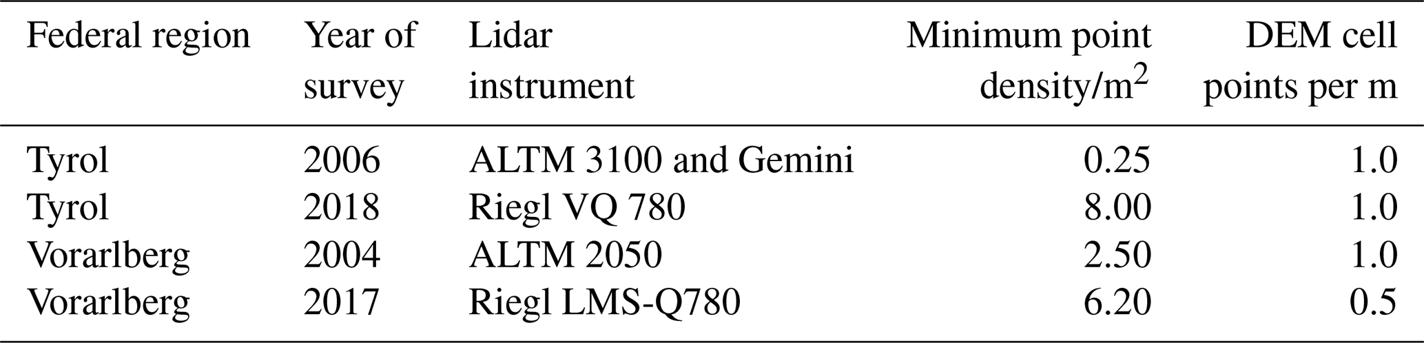
Lidar surveys using different instruments and point densities (Table 1) produce different representations of the actual surface even without real surface changes over time. Based on achieved point densities, the gridding method and resolution may add a misalignment of different DEMs of the same area. For this, lidar data are validated at defined reference areas. There is a tradition in glaciological remote sensing and photogrammetry to cross-check the DEM accuracy for glacier-covered areas in potentially stable areas without surface changes.
Table 1Instrument, minimum point density, and pixel size of the lidar campaigns used in this study for the calculation of volume changes.
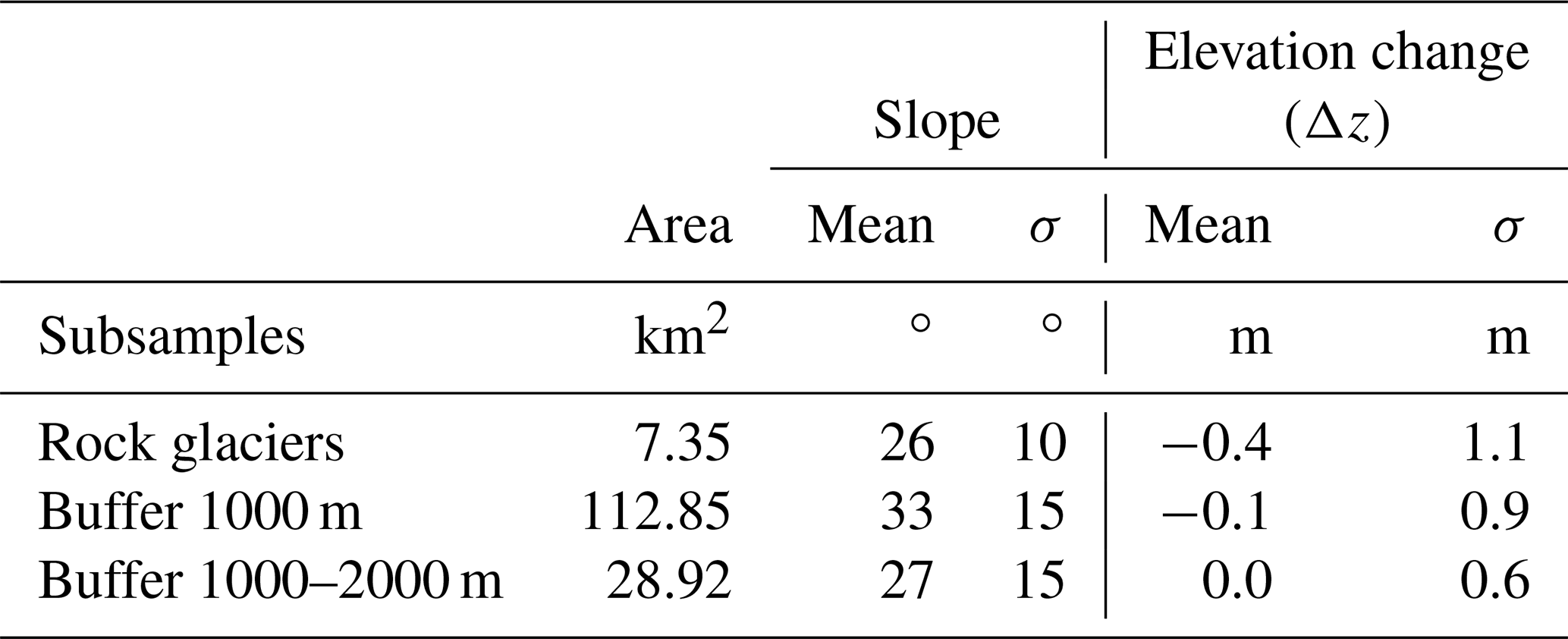
To estimate the final uncertainty with respect to changing point densities and methods applied for generating DEMs (Table 2), we analysed surface elevation changes (Δz) not only at glaciers but also at rock glaciers and for a buffer of 1000 m and between 1000 and 2000 m around all glaciers and rock glaciers. Although these areas are only partly representative of glaciers in terms of slope (Fig. 6) and roughness, we consider these numbers a very conservative estimate for the uncertainty of the Δz at glaciers. For the rough and changing rock glaciers, we found a mean Δz of −0.4 m with a standard deviation of 1.1 m. In the 1000–2000 m buffer, we found a mean elevation difference of 0.0 ± 0.6 m. The standard deviation is twice the uncertainty found by Abermann et al. (2010) for lidar DEMs. We took the standard deviation as error in Δz for further error propagation.
Table 2Comparison of the slope and elevation change (mean, standard deviation) between 2004/2006 and 2017/2018 for three subsamples.
Studies on the derivation of DEMs from lidar point clouds reveal that at slopes steeper than about 40∘, it potentially exhibits larger deviations from the actual surface (Sailer et al., 2014). Although the algorithm applied to convert point clouds to gridded data plays a major role in the representation of a specific surface (elevation and shape), the representation of the smooth glacier surfaces is a bit more resilient to low resolution than very rough geomorphological features. Sailer et al. (2014) claim that the cell size for analysing glacier changes could be even between 5 and 10 m.
Sailer et al. (2014) recommend cell sizes below 1 m for terrain steeper than 40∘, which we rarely find on the glaciers of the Austrian Silvretta, where 90 % of the glacier area has slopes below 40∘ (Fig. 6). In any case, the spatial resolution of the lidar DEMs analysed in this study fulfils the criteria above.
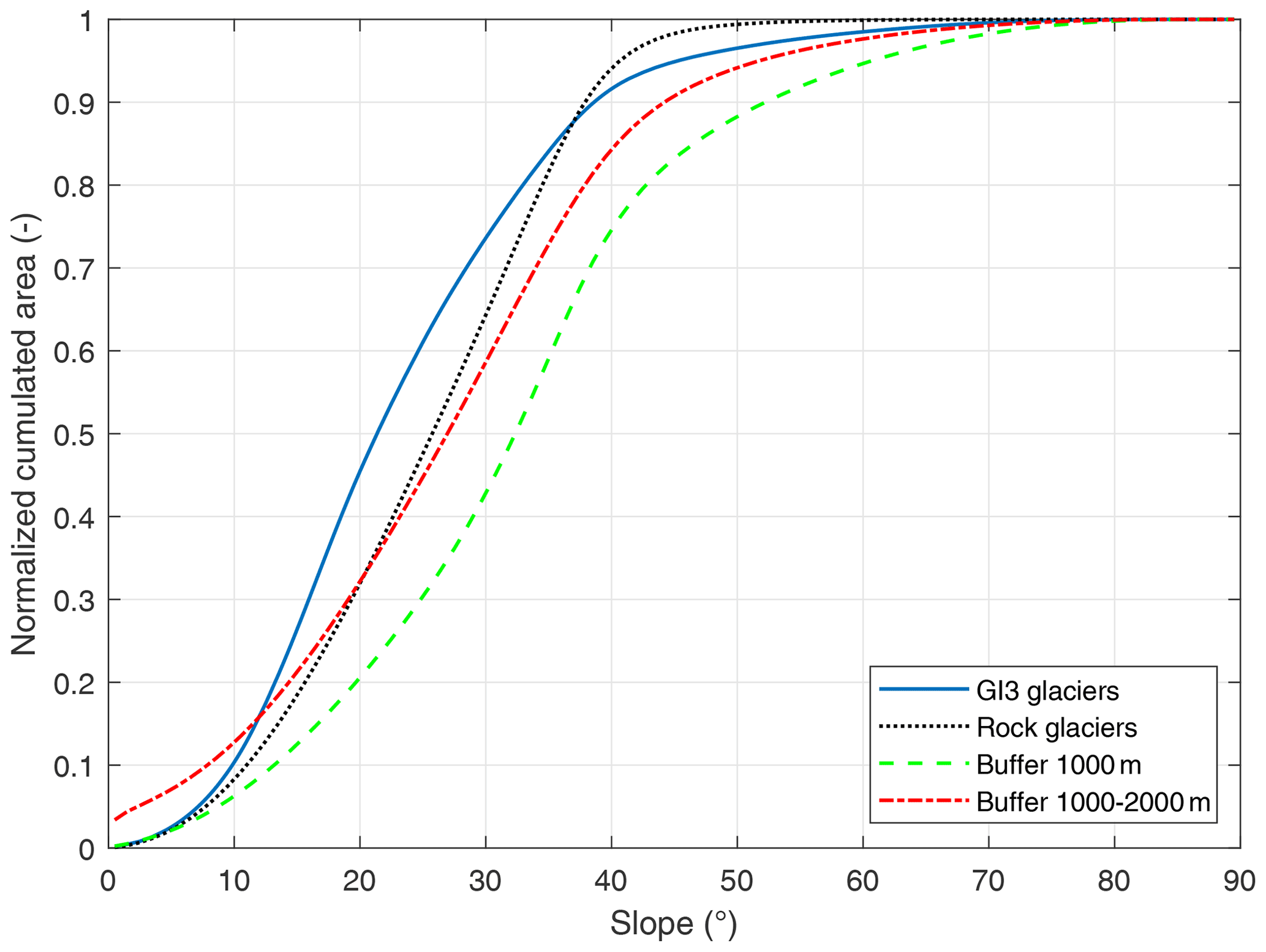
Figure 6Distribution of slopes for glaciers, rock glaciers and the two buffer areas used for validation. The buffer regions are steeper than the glaciers, so that the elevation difference in the stable buffer zones can be considered an upper limit for the uncertainty.
3.1 Compilation of the glacier inventory 2017/2018
We have mapped the glacier outlines manually based on the high-resolution lidar shaded reliefs and volume changes generated from lidar DEMs (Abermann et al., 2009) with 1×1 m pixel size as shown in Fig. 7 for Schnapfenkuchl M terminus. The full work flow is shown in Fig. 8. The shaded reliefs allow for an estimate of the glacier outline by distinguishing the smooth glacier areas from the rougher peri- and paraglacial areas. The characteristic patterns of elevation changes reaching their maximum at the glacier terminus help to include debris-covered glacier areas as well.
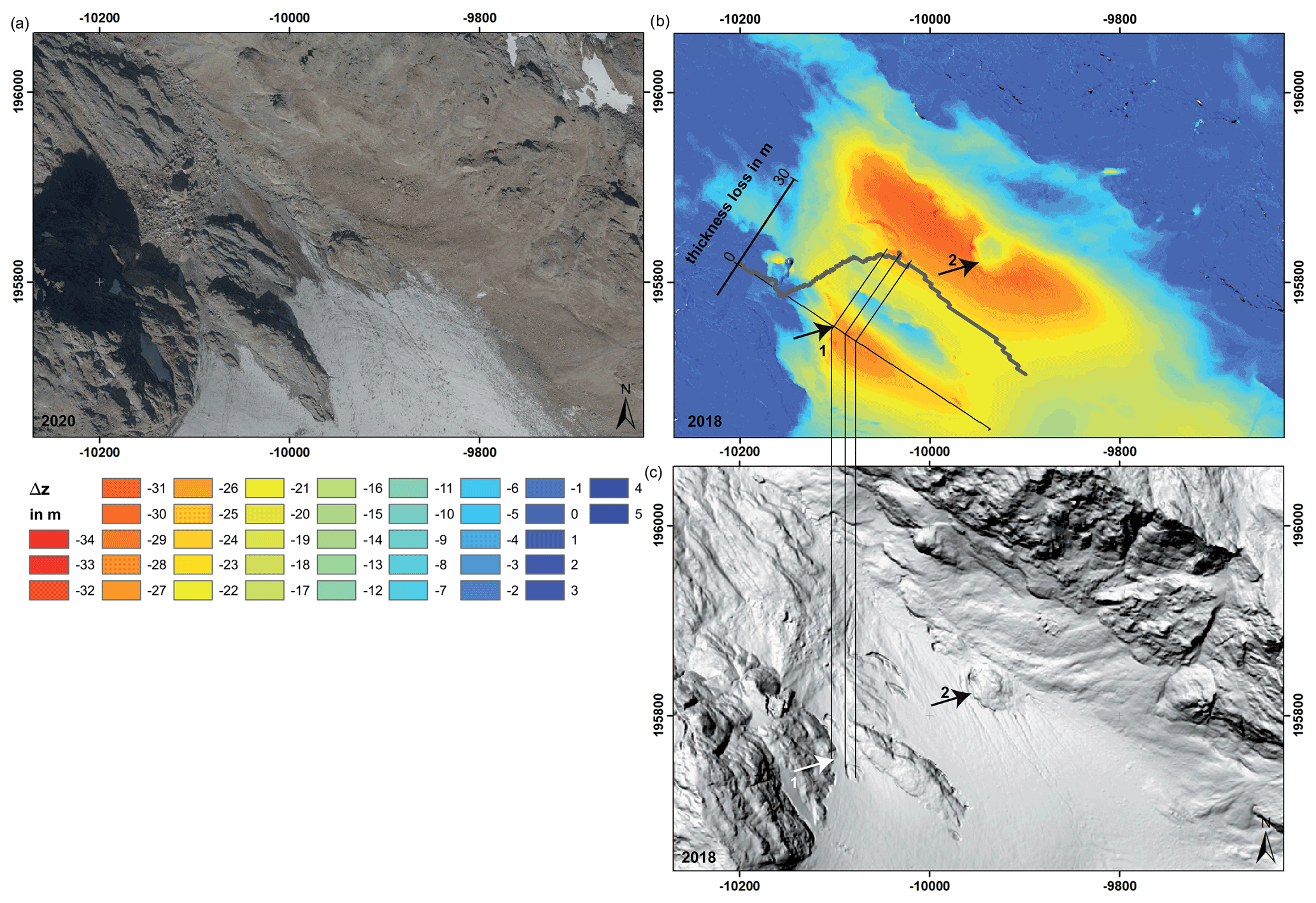
Figure 7The glacier margins of Schnapfenkuchl M terminus illustrated in the 2020 orthophoto (a) was mapped from thickness changes (Δz) between 2004 and 2017 (b). A characteristic pattern of thickness loss indicates the position of the glacier terminus and rock outcrops: the total thickness loss of areas where the ice is gone between t1 and t2 is smaller than that for the ice margin at t2 (position at t2 indicated by the arrows 1 and 2). The hillshade of the 2018 DEM (c) provides an additional source of information as the glacier surface tends to be smoother than the surrounding area. Source orthophoto: CC 4.0 https://www.data.gv.at/katalog/en/dataset/orthofoto.
The identification of areas with subsidence by melt is a clear advantage of this technology and allows glacier areas to be mapped that are hard to identify in orthophotos or visible remote-sensing data. In a validation step, orthophotos (acquired at different dates) were used for a consistency check of the lidar-derived outlines.
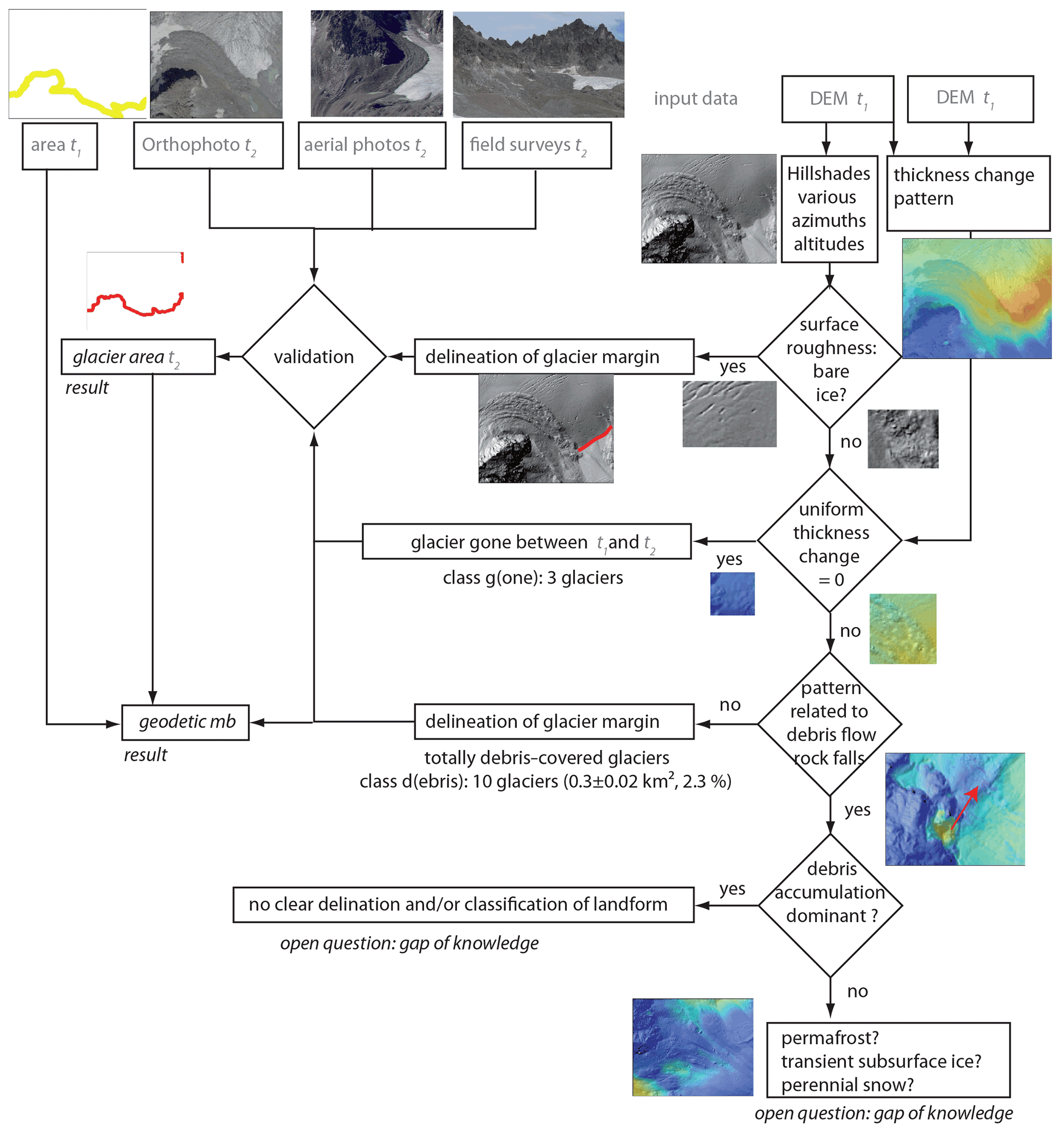
Figure 8Summary of the workflow for high-resolution glacier mapping and mass balance calculation for the period t1 to t2 as applied in this study. The workflow does lead to quantitative results for most of the glaciers but also shows the need of scientific discussion on geomorphological processes other than ice melt contributing significantly to volume changes. See Fig. 7 for the colour table of the volume change maps displayed (photos: Andrea Fischer; geodata: source Land Tirol).
Several past glacier inventories use a minimum size threshold, as compiled by Leigh et al. (2019) based on the spatial resolution of the remote-sensing data used. In this study, as for all previous Austrian glacier inventories, we applied no minimum size to mapping the glaciers. Only 4 of the 46 glaciers mapped were larger than 1 km2 in 2002, and two of the glaciers were smaller than the 0.01 km2 recommended by Paul et al. (2009) as a practical lower limit for mapping mountain glaciers by remote sensing.
3.2 Calculation of the volume change
The volume change for each pixel was calculated by multiplying the Δz with the 1 m2 pixel area A. For the total volume change ΔV of a glacier, the volume changes of all pixels within the glacier margins of the first date (t1) of the period t1 to t2 (Eq. 1) were summed up.
The maximum uncertainty of Δz at one pixel is the sum of the uncertainties in the elevations of both DEMs involved. The uncertainty in area adds to the uncertainties in Δz for the uncertainty of the total volume change.
Presuming that the thickness change Δz and the area change ΔA are independent variables, the uncertainties in glacier-covered area and thickness change propagate to the volume change uncertainty (Eq. 2).
3.3 Calculation of the geodetic mass balance
The geodetic mass balance Bgeo was calculated from volume change, assuming a constant glacier density ρ of 850 kg/m3 (Eq. 3).
Calculating the geodetic mass balance from the volume change requires assumptions on the stability of the glacier bed and on the density of the volume lost or gained. Erosion and deposition of sediments at the glacier bed were neglected for this study as research on the quantification of volumes is still ongoing. Previous studies on Austria's mass balance glaciers used a constant density of 850 kg/m3 and so did Fischer et al. (2015c) for the Swiss glaciers.
In recent years, the firn cover has melted completely. Thus the density at the surface may be higher. At the same time, ice flow velocities have slowed down (Stocker-Waldhuber et al., 2019). This has resulted in the formation of englacial cavities (Stocker-Waldhuber et al., 2017) which reduce the average density at the glacier tongues. The spatial and temporal variability in glacier density σρ is expressed in an uncertainty of ±60 kg/m3. Rocks, debris, and sediments on and within the glacier are treated as being part of the glacier.
The annual area-averaged specific geodetic mass balance bgeo is then calculated in two ways: (i) dividing the geodetic mass balance Bgeo by the area of the glacier at the beginning of period t1 and by the number of years (t2−t1) and (ii) dividing the geodetic mass balance Bgeo by the average of the glacier in the period t1 to t2 and by the number of years (t2−t1).
The uncertainty of the annual area-averaged specific mass balance is then defined as (Eq. 7)
where both potential definitions of the area, as area at the beginning of the period (Eq. 5) and as average area within the period (Eq. 6), were applied.
4.1 Total area and volume changes
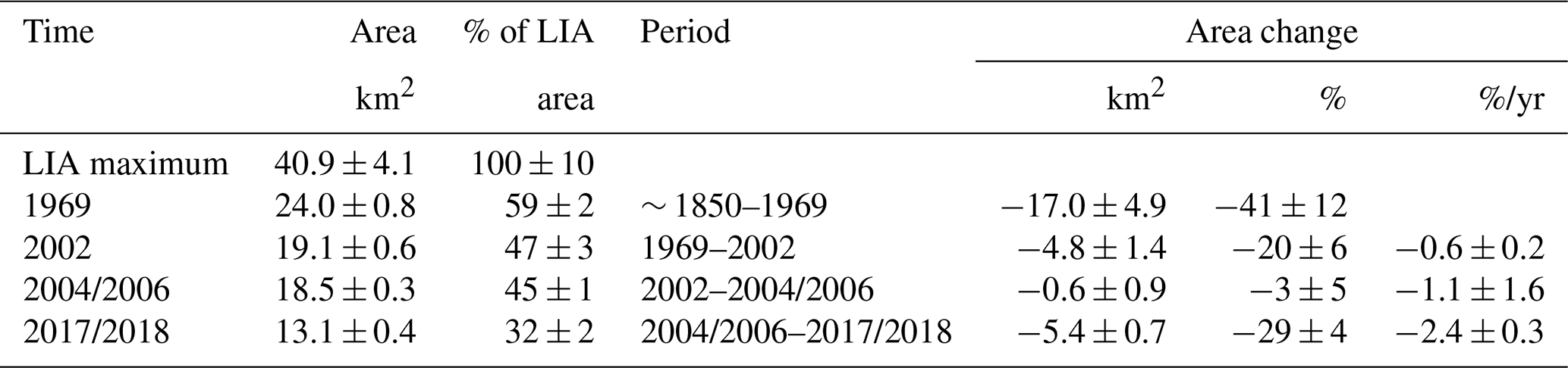
From the LIA maximum ∼1850–2017/2018, the Austrian Silvretta lost 68 % of its glacier area (Table 3, Fig. S4). The mean annual area loss in the latest period was 2.4 %, which is more than twice the loss of the period before. The 10 totally debris-covered glaciers cover an area of 0.303 km2 (Table S3). For three glaciers (ID 13006, Fluchthornferner S, and Litzner Gletscher E), neither bare ice nor signs of motion or a drainage system were visible, and mean thickness changes between 2004/2006 and 2017/2018 were smaller than 2.6 m without a clear thickness change pattern to indicate an ice margin. From that we can conclude that the subsurface ice melted.
Area changes were calculated for all glaciers for the periods of the LIA maximum ∼1855–1969 and 1969–2002 (Table 3). The dates of lidar campaigns differ between the federal states of Vorarlberg (2004 and 2017) and Tyrol (2006 and 2018). Later periods are thus 2002–2004/2006 and 2004/2006–2017/2018.
Table 3Glacier area in the Austrian part of the Silvretta between LIA maximum, 1969, 2002, 2004/2006, and 2017/2018. For Vorarlberg, lidar flights were carried out in 2004 and 2017 and for Tyrol in 2006 and 2018.
The annual specific geodetic mass balance (Table 4) was most negative in the short period with the extreme summer of 2003 (−1.5 ± 0.7 m w.e./yr), and least negative in the period 1969–2002 (−0.2 ± 0.1 m w.e yr). That geodetic mass balance in the latest period is less negative in magnitude than in the short period before can be attributed to the loss of ablation area within the period. The overall volume loss is reduced despite increasing ablation rates at the stakes because the areas with highest ablation rates in the past are ice-free now. The most negative glacier-wide specific mass balance was recorded in 2015 (Fischer et al., 2016c).
Table 4Glacier volume loss, geodetic balance (total, specific, and specific annual) in the Austrian part of the Silvretta between 1969, 2002, 2004/2006, and 2017/2018. For Vorarlberg, lidar flights were carried out in 2004 and 2017 and for Tyrol in 2006 and 2018.

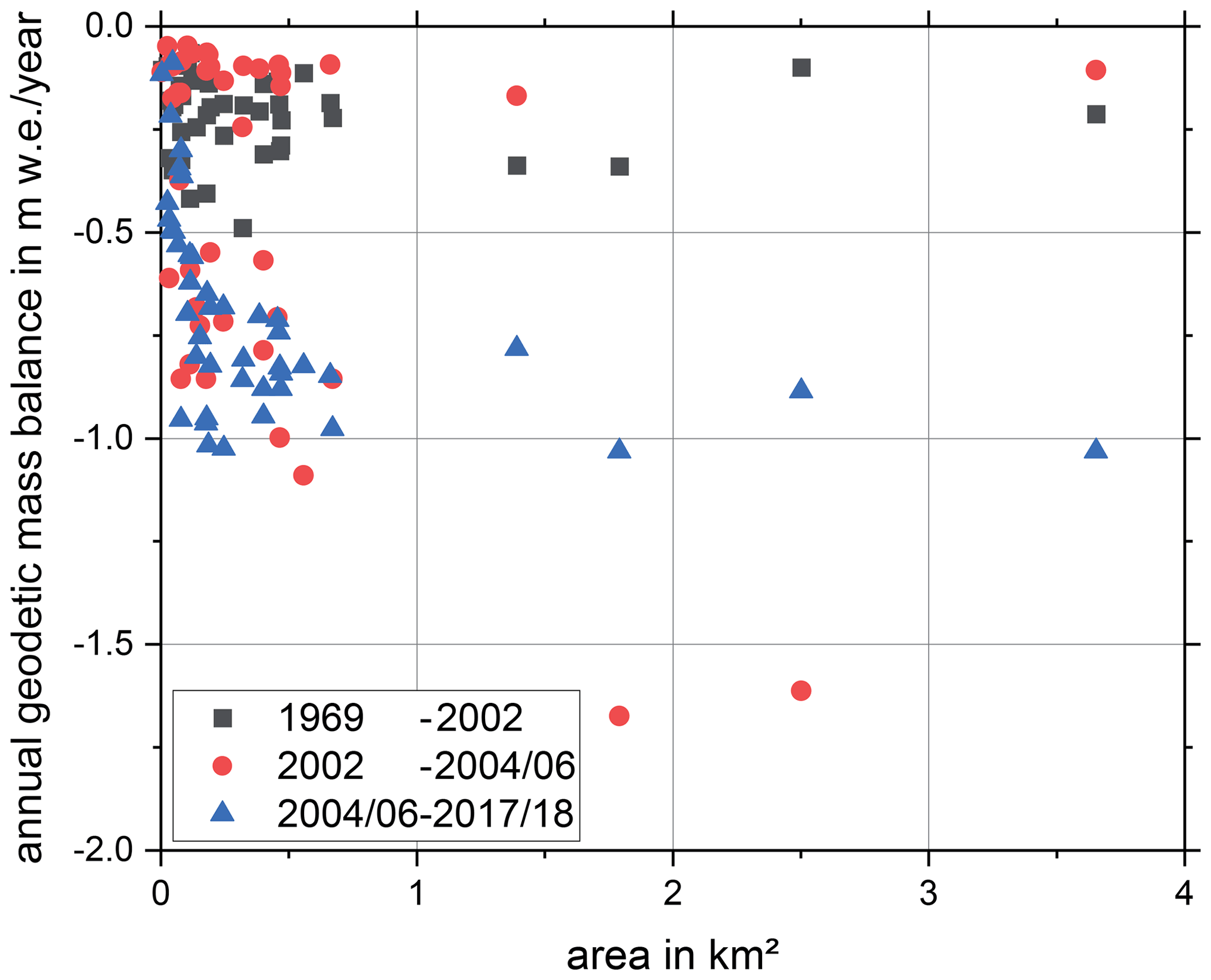
Figure 9Annual geodetic mass balances for the Austrian Silvretta in 1969–2002, 2002–2004/2006, and 2004/2006–2017/2018.
4.2 Volume changes and geodetic balance for individual glaciers
For individual glaciers, the three inventories also show strongest annual losses for the short period with the extreme year 2003 (Fig. 9, Table S1), lowest annual losses for all glacier sizes in the period 1969–2002, and medium losses for the latest period. Glaciers with smaller areas present the highest variability. In contrast to the short and first warm inventory period 2002–2004/2006, when some of the smaller glaciers were still quite stable, the range of geodetic mass balance for small glacier sizes is high, from losses of more than 1 m w.e./yr to a few glaciers with quite stable conditions, which is related to debris cover (or total loss of ablation area).
4.3 Influence of area reference on geodetic balance
The choice of the area, either the area at the beginning of the period or the average area within the period, has an impact on the geodetic mass balance, changing annual balance by up to 0.33 m w.e./yr for individual glaciers (Table S2). The geodetic balance becomes more negative if related to the average area by −0.16 m w.e./yr. This also reveals that it is not only a neglect of debris-covered glacier areas but also the wrong inclusion of debris-covered areas without ice that can affect the uncertainty of geodetic mass balance estimates.
5.1 Challenges for mapping area changes in disintegrating glaciers
With ongoing glacier disintegration, mapping glacier outlines becomes ever more ambiguous even if using high-resolution volume change data. Major points to discuss are as follows:
-
What exactly are the properties that make a cryogenic feature a glacier which should be included in a glacier inventory?
-
Should we introduce inventories of all cryogenic features including glaciers, permafrost, and rock glaciers?
-
Do we need to define a point of glacier disappearance?
All glaciers in this study were mapped first in previous inventories at times when bare ice was largely visible. For the now totally debris-covered glaciers, it is hard to decide using only optical data whether there is any ice left. In the absence of bare ice or surface structures, such as ponds or crevasses, and with soft slopes and low potential velocities, surface velocities do not help to distinguish buried glaciers from rock glaciers and permafrost dynamics. As measurements in bore holes in rock glaciers show, sliding debris and rocks on the ice can account for a major part of the total surface velocity (Krainer et al., 2015). If a subsurface run-off system exists at the terminus, it is necessary to analyse if it is fed by groundwater, melt of seasonal snow, permafrost ice, or glacier ice. This can be done by analysing the seasonality of the amount of run-off (e.g. Brighenti et al., 2019), chemical composition, and ecological properties (e.g. Tolotti et al., 2020), as well as by isotope analysis of the meltwater (e.g. Wagenbach et al., 2012).
Careful analysis is needed to decide whether a formerly well-defined glacier still fulfils the criteria of a glacier. Taking glaciers off inventories prematurely is to be avoided as they may still contribute to glacial run-off in the basin, can force debris slide, or serve as essential climate variables. We lose track of these transient states by dropping these glaciers from the inventories.
5.2 Uncertainties in mapping totally debris-covered glaciers
Mapping glaciers that have become fully covered with debris is uncertain for two reasons. First, mapping areas of possible ice covered with debris by volume changes only allows the presence of melting ice to be tackled during the inventory period, but it does not prove that any ice is left at the end of the period. Second, the presence of melting ice is not restricted to debris-covered glaciers but is also true for permafrost. The Schnapfenkuchl glaciers V and H present glacier ice at locations where debris flows exposed the ice and past inventories showed bare ice.
The Schnapfenkuchl glaciers are embedded in an environment adjacent to a number of rock glaciers (Fig. 10). The delineation of buried glaciers in the presence of permafrost and mass movements upon and from the glacier needs a high temporal frequency of inventory data to arrive at the detection of glacier ice. High spatial resolution is needed to distinguish between ice loss and ice dynamics and to track the geomorphological processes and features related to volume change.
Surface elevation changes result from ice volume changes but also from relocation, accumulation, or erosion of supraglacial, englacial, or subglacial debris. The related geomorphological processes can be tackled by characteristic patterns of volume changes. The higher the temporal resolution of the repeat imagery, the more clearly can individual events be distinguished.
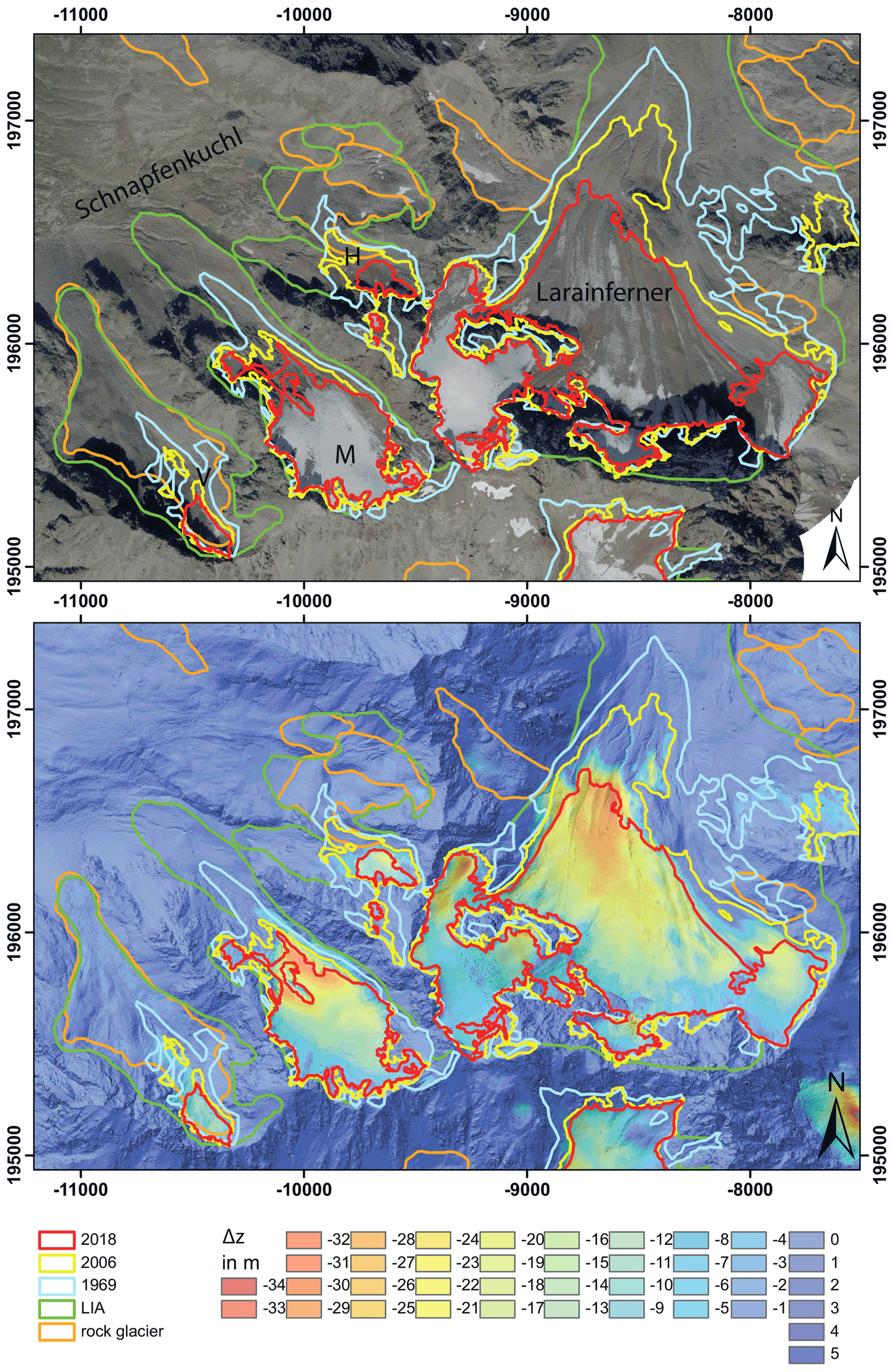
Figure 10Final glacier outline 2018 and thickness changes 2006–2018 for the Schnapfenkuchl glaciers V, M, and H and Larainferner displayed on (a) the orthophoto from 2020 and (b) the elevation changes from 2006–2018 superimposed on the hillshade of 2018. Source orthophoto: CC 4.0 https://www.data.gv.at/katalog/en/dataset/orthofoto.
5.3 Comparison to remote-sensing results
The Sentinel-2-based inventory of the Alps (Paul et al., 2020) is based on data of exactly the same year, 2018, as the Tyrolean lidar inventory; for Vorarlberg acquisition dates differ by 1 year. This is an opportunity to compare the representation of different types of glaciers in the various data sets, as shown for Landsat 8 (9 September 2018, 30 m resolution), Sentinel-2 (9 September 2018, 10 m resolution), and lidar data (2018), as well as orthophotos (2020), for the bare ice snout of Schnapfenkuchl M (Fig. 11) and the totally debris-covered Schnapfenkuchl H (Fig. 12). While clean ice can be easily mapped, the identification of debris-covered glaciers like Schnapfenkuchl H is more challenging in all types of optical imagery, independent of the pixel spacing. Although higher-resolution optical imagery allows for the detection of features potentially related to subsurface deformation, the potential for the quantification of the ice extent is limited. Volume change allows for only the detection of the past presence of ice and not the proof of the actual current presence of ice. The regional comparison of change rates can also give a hint of the total melt within the period as in this case the volume change rate is lower than in similar settings with a permanent presence of ice.
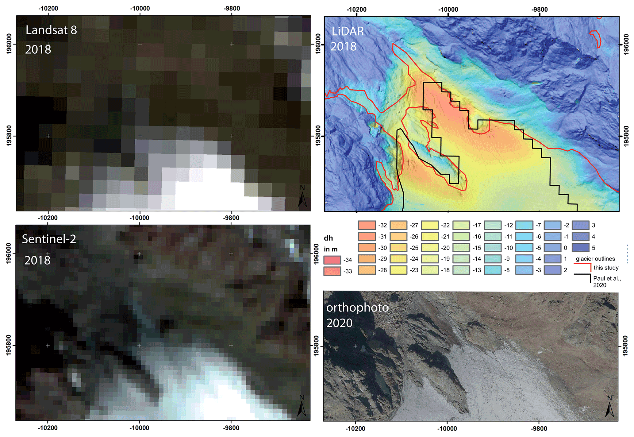
Figure 11The comparison of the Landsat 8, Sentinel-2, and lidar images (hillshade and volume change 2006–2018, colour map like in Fig. 10), all dating from 2018, and the orthophoto (2020) illustrates the different representation of the glacier in the various spatial resolutions for the snout of Schnapfenkuchl M. For glaciers with bare ice, glacier margins are clear at all scales of resolutions.

Figure 12Representation of the debris-covered glacier Schnapfenkuchl H in the Landsat 8, Sentinel-2, and lidar images (hillshade and volume change 2006–2018, colour map like in Fig. 10) and the orthophoto. The manual delineation of glacier outlines (red: based on lidar; black: based on Sentinel-2; Paul et al., 2020) is consistent for both methods.
For the total region, the Sentinel-based glacier area is 13.035 km2, therefore only 0.098 km2 smaller than the lidar-based inventory, both listing 46 glaciers. Part of the consistency of the inventories results from the fact that both are based on the same older glacier inventory and that both observers also focused on consistency with this inventory. Therefore, the compilation of time series of inventories as homogenous as possible could be a major advantage for precision even in the absence of high-resolution data.
5.4 Should we still map small and totally debris-covered glaciers?
Past definitions of glaciers focussed on the mass of ice. From the earliest definitions, e.g. by Walcher (1773) and Tyndall (1860), to more modern ones within glaciology (von Klebelsberg, 1948; Cogley et al., 2011; Raup and Khalsa, 2010) and in neighbouring fields (Dexter, 2013), scientists have obviously been investigating glaciers closer to equilibrium than those in our study (definitions cited in the Supplement). The more modern definitions of Cogley et al. (2011) and Raup and Khalsa (2010) address the need of the glaciological community for mapping glaciers mainly based on remote-sensing data.
Although englacial and supraglacial debris was present on and in glaciers even during the LIA, ice and snow dominated at the time. In our glacier inventory of 2017/2018, 10 of 43 glaciers are predominantly covered by debris, not snow, with only a few remnants of bare ice visible. Mean thickness changes range from −1.5 ± 0.1 to −12.3 ± 0.6 m for 2004/2006–2017/2018. Several of the debris-covered glaciers, for example, the Schnapfenkuchl glaciers (Fig. 10), are located between active rock glaciers captured in the Tyrolean rock glacier inventory (Krainer and Ribis, 2012). This means that two independent groups of researchers, glaciologists and geologists, mapped the same site, for example, the easternmost Schnapfenkuchl glacier/rock glacier, in inventories of different landforms. A continuum from glacier to debris-covered glacier to rock glacier was recently discussed by Anderson et al. (2018). Kellerer-Pirklbauer and Kaufmann (2018) analysed the glacial history of an Austrian site of long-term rock glacier monitoring and found evidence of post-LIA deglaciation to permafrost formation. For the broader scientific investigation of this phenomenon, international cooperation for comparing processes and regimes in other mountain regions is vital since a case study can only be a first step towards deriving more general empirical and theoretical knowledge.
More concise definitions of the term glacier are needed to reflect current conditions on the ground. We suggest the following possibilities:
-
Glaciers are bodies of sedimentary ice, firn, and snow, formed by densification of snow AND englacial and supraglacial sediments of all grain sizes.
-
Glaciers are exposed bodies of sedimentary ice, firn, and snow formed by densification of snow with signs of deformation and an englacial or supraglacial drainage system.
Definition (1) includes all sizes of ice bodies which have been formed as part of glaciers, even dead debris-covered glacier ice and ice-cored moraines. It understands debris as a natural part of the glacier system, also in the calculation of volume changes, and sets down a clear base for mapping glaciers in inventories and calculating geodetic balances. Mapping internal properties as englacial deformation or the existence of drainage systems often is not possible by remote sensing, and the advantage of definition (1) is that there is no need to do so. The drawback is that including debris accepts that glacier volume changes are not necessarily ice volume changes. This accounts for the problem that it is not possible to assess the amount of englacial debris anyway.
Definition (2) excludes dead and buried glacier ice, which might have advantages for mapping, especially in low resolutions, but leaves an undefined gap between glaciers and permafrost ice, thereby introducing a third class, i.e. buried glacier ice.
Janke et al. (2015) propose a gradual transition between debris-covered and buried ice with still ongoing melt and respective volume loss for the ice buried by 3–5 m of debris. As criteria for the classification as rock glacier, they apply a complete debris cover with no ice visible at the surface and a less heterogeneous internal structure with glacier ice, segregated ice, and interstitial ice. The ice content varies between 25 % and 45 %. Predominant surface features are thermokarst depressions and transverse ridges and furrows. This classification is definitely valuable for mapping glaciers and rock glaciers, but the traditional Austrian rock glacier and glacier inventories have been using other types of classifications, e.g. including parts of bare ice in the rock glacier inventory. The coming years or decades will show if the transient features in the Austrian Silvretta can develop ridges or furrows, or if the ice is gone before these structures evolve.
5.5 Comparison of changes in the Austrian Silvretta with other glacier regions
For the Austrian Silvretta, the mean annual geodetic balance is −0.8 ± 0.1 m w.e./yr for the period from 2004/2006 to 2017/2018. This is less negative than the −1.03 m w.e. reported for the Glarus and Leopoldine Alps by Sommer et al. (2020) for the period from 2000 to 2014, but it is a greater loss than the −0.62 m w.e./yr calculated by Fischer, Huss, and Hoelzle (2015c) for the Swiss Alps between 1980 and 2010. They also reported a variability in geodetic balances on the catchment scale, ranging from −0.52 to −1.07 m w.e. Our data confirm the highly variable sensitivity of small glaciers to warming as found by Huss and Fischer (2016).
The annual rate of area losses in the Austrian Silvretta (1969–2017/2018) of −1.13 % is larger than the −0.52 % reported for a slightly shorter period (1986–2014) in the Caucasus (Tielidze et al., 2020) but similar to the −1.1 % reported by Paul et al. (2020) for the Alps between 2003 and 2015/2016 excluding glaciers smaller than 0.01 km2.
Although the respective regions are very different in terms of elevation range, climate, and glacier cover, the glacier mass loss is strikingly similar.
For mapping small glaciers in Norway, Leigh et al. (2019) developed a rating system, classifying glaciers from “certain” to “probable” based on < 1 m resolution visible imagery. The scoring is based on visible features like ogives, crevasses, and moraines. In the absence of volume change data, this might be a helpful approach to keep track of buried glacier ice.
5.6 Additional uncertainties of geodetic mass balance
Geodetic mass balance has been analysed for potential uncertainties, for example, unaccounted seasonal snow interpreted as ice volume change or changing glacier beds, and real mass changes differing from surface mass balance, for example, as a result of refreezing, firn density changes, or crevasse volume (e.g. Zemp et al., 2013). For the very small and debris-covered glaciers we analysed, an additional source of uncertainty is the amount of the accumulated debris on the surface. This volume is not part of the hydrological cycle, so, from a hydrological perspective, we would wish to exclude this volume from the analysis. This would be possible only if we could keep track of the erosion rates in the source areas. This would necessitate a totally different monitoring system to track the steep headwalls. In terms of geomorphology, debris and rocks are part of the glacier, and therefore there is no need to distinguish old from new supra- and englacial debris and rock.
The rougher surface at steep debris-covered glaciers with avalanche activity seems to encourage the formation of perennial snow patches on the debris-covered glacier. This is not relevant for delineating glaciers but raises the question on the effects of these perennial snow volumes on geodetic mass balance. This question could also be answered with a specific monitoring effort tackling the now-stored volumes and water equivalents. In this effort first hints on potential ice formation in such structures could be gathered.
The annual rates of change in area and volume indicate an increasing pace of glacier retreat in the Austrian Silvretta. A growing number of nunataks, the disintegration of larger glaciers into smaller ones, and the accumulation and relocation of debris on the glacier surface all indicate an additional need for compiling glacier inventories – if we want to keep track of buried glacier ice. For most of the 46 glaciers, the procedure of delineating the glacier surface by surface roughness and volume change validated by orthophotos worked out well, even for the 10 glaciers totally covered by debris. However, for some of the analysed glaciers, for example Schnapfenkuchl V, future analysis of areas will be difficult as the surface is now totally covered with debris, and the accumulation and relocation of the debris are still ongoing. Therefore, we cannot expect a distinct pattern of thickness change in the future with a maximum close to the terminus. In the next decade we thus need a scientific discussion on how to proceed with as yet undefined subsurface glacier remnants.
The technical requirements for mapping small vanishing glaciers depend on glacier size, annual rate of thickness changes, and accumulation rates of debris. The small glacier structures that remain in the Austrian Silvretta are typically just a few tens of metres wide. With increasing pixel size, the accuracy of mapping vertical changes decreases, which makes it difficult to distinguish geomorphological processes like accumulation and relocation of rocks and debris from ice volume change. Therefore, we recommend 1 m spatial resolution. The vertical accuracy needed to represent the geomorphological processes of debris relocation depends on the steepness of the area and on the temporal interval chosen. For a period of 10 years and a slope of up to 40∘ for Alpine glaciers, a vertical resolution of of the spatial resolution is sufficient to distinguish volume changes by ice melt from erosion and deposition.
Of the now 43 glaciers of the Austrian Silvretta, only 3 are larger than 1 km2, and 19 are smaller than 0.1 km2 (of these, 13 are smaller than 0.05 km2). Applying minimum sizes for glacier area with thresholds at 0.1 or 0.05 km2 would exclude 0.82 km2/6.2 % and 0.35 km2/2.7 % of the total area. This is higher than in the same magnitude as the nominal uncertainty of 0.4 km2 in the total area. Such thresholds for very small glaciers would make many of them disappear from inventories and hamper any efforts to tackle the hazard potential of deglaciation as even small glacier remnants could be relevant here.
There is probably no hard limit for surveying deglaciation in terms of glacier size as the monitoring strategies for rock glaciers and permafrost can take over. Handing over what is left from glaciers to the scientific networks of the permafrost community could be an emerging and exciting new playground for both fields.
This regional study can only point out the specific challenges and limitations for tackling glacier change in the Austrian Silvretta. These will differ from region to region depending on the climatic regime, lithology, topography, glacier types, and many other factors. We would therefore appreciate an international effort to compare the need for tackling deglaciation in other regions as a common monitoring framework will be essential in an ever warmer future.
The glacier inventory data are available at https://doi.org/10.1594/PANGAEA.844988 (Fischer et al., 2015b) and https://doi.pangaea.de/10.1594/PANGAEA.936109 (Fischer et al., 2021).
The video supplements show the down waste of the Schnapfenkuchl glaciers and Larainferner (https://doi.org/10.5446/53743, Fischer, 2021a) and a close up of the evolution of Schnapfenkuchl H glacier (https://doi.org/10.5446/53742, Fischer, 2021b) and of the retreats of Bieltalferner glacier, Verhupf glacier, Litzner glacier, and Fluchthornferner glacier (https://doi.org/10.5446/43410, https://doi.org/10.5446/53943, https://doi.org/10.5446/53923, https://doi.org/10.5446/53882; Fischer, 2021c, d, e, f).
The supplement related to this article is available online at: https://doi.org/10.5194/tc-15-4637-2021-supplement.
AF designed this study, worked on glaciers in the Silvretta range for over a decade, and wrote the text. KH, BS, and MSW analysed the geodetic data, and GS contributed remote-sensing data and expertise. All authors contributed to the discussion and text.
The authors declare that they have no conflict of interest.
Publisher’s note: Copernicus Publications remains neutral with regard to jurisdictional claims in published maps and institutional affiliations.
The federal administrations of Tyrol and Vorarlberg are acknowledged for providing geodata. Open government geodata were used with CC4 licence (Land Tirol – data.tirol.gv.at) and CC3 licence (Land Vorarlberg – data.vorarlberg.gv.at). We thank the community of Galtür, the Lorenz family at Jamtalhütte, and Oswald Heis for supporting logistics. Kati Heinrich helped with the figures, and Brigitte Scott checked the English – thank you! We thank the three anonymous reviewers and the editor Louise Sandberg Sørensen for their helpful comments and suggestions.
Both lidar DEMs were provided by the TIRIS section of the federal administration of Tyrol and the federal administration of Vorarlberg.
This paper was edited by Louise Sandberg Sørensen and reviewed by three anonymous referees.
Abermann, J., Lambrecht, A., Fischer, A., and Kuhn, M.: Quantifying changes and trends in glacier area and volume in the Austrian Ötztal Alps (1969–1997–2006), The Cryosphere, 3, 205–215, https://doi.org/10.5194/tc-3-205-2009, 2009.
Abermann, J., Fischer, A., Lambrecht, A., and Geist, T.: On the potential of very high-resolution repeat DEMs in glacial and periglacial environments, The Cryosphere, 4, 53–65, https://doi.org/10.5194/tc-4-53-2010, 2010.
Anderson, R. S., Anderson, L. S., Armstrong, W. H., Rossi, M. W., and Crump, S. E.: Glaciation of alpine valleys: The glacier – debris-covered glacier – rock glacier continuum, Geomorphology, 311, 127–142, https://doi.org/10.1016/j.geomorph.2018.03.015, 2018.
Bahr, D. B. and Radić, V.: Significant contribution to total mass from very small glaciers, The Cryosphere, 6, 763–770, https://doi.org/10.5194/tc-6-763-2012, 2012.
BEV: Höhen-Grid plus Geoid, available at: https://www.bev.gv.at/portal/page?_pageid=713,2363167&_dad=portal&_schema=PORTAL (last access: 23 September 2021), 2011.
Bojinski, S., Verstraete, M., Peterson, T., Richter, C., Simmons, A., and Zemp, M.: The Concept of Essential Climate Variables in Support of Climate Research, Applications, and Policy, B. Am. Meteorol. Soc., 95, 1431, https://doi.org/10.1175/BAMS-D-13-00047.1, 2014.
Braumann, S. M., Schaefer, J. M., Neuhuber, S. M., Reitner, J. M., Lüthgens, C., and Fiebig, M.: Holocene glacier change in the Silvretta Massif (Austrian Alps) constrained by a new 10Be chronology, historical records and modern observations, Quaternary Sci. Rev., 245, 106493, https://doi.org/10.1016/j.quascirev.2020.106493, 2020.
Brighenti S., Tolotti M., Bruno M. C., Wharton G., Pusch M. T., and Bertoldi W.: Ecosystem shifts in Alpine streams under glacier retreat and rock glacier thaw: a review, Sci. Total Environ., 675, 542–559, https://doi.org/10.1016/j.scitotenv.2019.04.221, 2019.
Cogley, J. G., Hock, R., Rasmussen, L. A., Arendt, A. A., Bauder, A., Braithwaite, R. J., Jansson, P., Kaser, G., Möller, M., Nicholson, L., and Zemp, M.: Glossary of glacier mass balance and related terms, Paris, UNESCO/IHP, https://doi.org/10.5167/uzh-53475, 2011.
data.tirol.gv.at: Current and historical orthoimagery of Tyrol, Open government data, available at: https://www.data.gv.at/katalog/dataset/land-tirol_orthofototirol, last access: 23 September 2021.
Dexter, L. R. and Birkeland K. W.: Snow, Ice, Avalanches, and Glaciers, in: Mountain Geography: Physical and Human Dimensions, edited by: Price, M. F., Byers, A. C., Friend, D. A., Kohler T., and Price, L. W., 1st ed., University of California Press, JSTOR, 85–126, available at: https://www.jstor.org/stable/10.1525/j.ctt46n4cj.10 (last access: 15 December 2020) 2013.
Federal Government of Tyrol: Landesweite Laserscanbefliegung 2006–2010, available at: https://www.tirol.gv.at/fileadmin/themen/sicherheit/geoinformation/Laserscandaten/ALS_Tirol_Onlinebericht.pdf, last access: 11 December 2020.
Fischer, A.: The evolution of the Schnapfenkuchl and Larain glaciers in the Austrian Silvretta 1954–2020, TIB AV Portal [video supplement], https://doi.org/10.5446/53743, 2021a.
Fischer, A.: The evolution of Schnapfenkuchl H glacier 1954–2020, TIB AV Portal [video supplement], https://doi.org/10.5446/53742, 2021b.
Fischer, A.: Bieltalferner Austrian Silvretta 1950–2020, TIB AV Portal [video supplement], https://doi.org/10.5446/43410, 2021c.
Fischer, A.: Verhupf glacier Austrian Silvretta 1950–2020, TIB AV Portal [video supplement], https://doi.org/10.5446/53943, 2021d.
Fischer, A.: Litzner glacier Austrian Silvretta 1950–2020, TIB AV Portal [video supplement], https://doi.org/10.5446/53923, 2021e.
Fischer, A.: Fluchthornferner Austrian Silvretta 1954–2020, TIB AV Portal [video supplement], https://doi.org/10.5446/53882, 2021f.
Fischer, A. and Kuhn, M.: Ground-penetrating radar measurements of 64 Austrian glaciers between 1995 and 2010, Ann. Glaciol., 54, 179–188, https://doi.org/10.3189/2013AoG64A108, 2013.
Fischer, A., Seiser, B., Stocker Waldhuber, M., Mitterer, C., and Abermann, J.: Tracing glacier changes in Austria from the Little Ice Age to the present using a lidar-based high-resolution glacier inventory in Austria, The Cryosphere, 9, 753–766, https://doi.org/10.5194/tc-9-753-2015, 2015a.
Fischer, A., Seiser, B., Stocker-Waldhuber, M., Mitterer, C., and Abermann, J.: The Austrian Glacier Inventories GI 1 (1969), GI 2 (1998), GI 3 (2006), and GI LIA in ArcGIS (shapefile) format, PANGAEA [data set], https://doi.org/10.1594/PANGAEA.844988 2015b.
Fischer, M., Huss, M., and Hoelzle, M.: Surface elevation and mass changes of all Swiss glaciers 1980–2010, The Cryosphere, 9, 525–540, https://doi.org/10.5194/tc-9-525-2015, 2015c.
Fischer, A., Patzelt, G., and Kinzl, H.: Length changes of Austrian glaciers 1969-2016. Institut für Interdisziplinäre Gebirgsforschung der Österreichischen Akademie der Wissenschaften, Innsbruck, PANGAEA [data set], https://doi.org/10.1594/PANGAEA.821823, 2016a.
Fischer, A., Helfricht, K., Wiesenegger, H., Hartl, L., Seiser, B., and Stocker-Waldhuber, M.: What Future for Mountain Glaciers? Insights and Implications from Long-Term Monitoring in the Austrian Alps, chap. 9, in: Developments in Earth Surface Processes, edited by: Gregory, B., Greenwood, and Shroder, J. F., Elsevier, 21, 325–382, https://doi.org/10.1016/B978-0-444-63787-1.00009-3, 2016b.
Fischer, A., Markl, G., and Kuhn, M.: Glacier mass balances and elevation zones of Jamtalferner, Silvretta, Austria, 1988/1989 to 2016/2017, Institut für Interdisziplinäre Gebirgsforschung der Österreichischen Akademie der Wissenschaften, Innsbruck, PANGAEA [data set], https://doi.org/10.1594/PANGAEA.818772, 2016c.
Fischer, A., Stocker-Waldhuber, M., Seiser, B., Helfricht, K., and Schwaizer, G.: Glacier inventory Austrian Silvretta 2017/2018, PANGAEA [data set], https://doi.pangaea.de/10.1594/PANGAEA.936109, 2021.
Gärtner-Roer, I., Nussbaumer, S. U., Hüsler, F., and Zemp, M.: Worldwide assessment of national glacier monitoring and future perspectives, Mt. Res. Dev., 39, A1–A11, https://doi.org/10.1659/MRD-JOURNAL-D-19-00021.1, 2019.
Geist, T. and Stötter, H.: First results of airborne laser scanning technology as a tool for the quantification of glacier mass balance. Proceedings, EARSeL workshop on observing our cryosphere from space:techniques and methods for monitoring snow and ice with regard to climate change, 11–13 März 2002, Bern, 2002.
geoland.at: The free geodata portal of Austria, available at: http://www.geoland.at, last acess: 23 September 2021.
Haeberli, W., Hoelzle, M., Paul, F., and Zemp, M.: Integrated monitoring of mountain glaciers as key indicators of global climate change: The European Alps, Ann. Glaciol., 46, 150–160, https://doi.org/10.3189/172756407782871512, 2007.
Höfle, B. and Rutzinger, M.: Topographic airborne LiDAR in geomorphology: A technological perspective, Z. Geomorphol., 55, 1–29, https://doi.org/10.1127/0372-8854/2011/0055S2-0043, 2011.
Huss, M. and Fischer, M.: Sensitivity of very small glaciers in the Swiss Alps to future climate change, Front. Earth Sci., 4, 34, https://doi.org/10.3389/feart.2016.00034, 2016.
Huss, M., Zemp, M., Joerg, P. C., and Salzmann, N.: High uncertainty in 21st century runoff projections from glacierized basins, J. Hydrol., 510, 35–48, 2014.
IPCC: IPCC Special Report on the Ocean and Cryosphere in a Changing Climate, edited by: Pörtner, H.-O., Roberts, D. C., Masson-Delmotte, V., Zhai, P., Tignor, M., Poloczanska, E., Mintenbeck, K., Alegría, A., Nicolai, M., Okem, A., Petzold, J., Rama, B., and Weyer, N. M., available at: https://www.ipcc.ch/site/assets/uploads/sites/3/2019/12/SROCC_FullReport_FINAL.pdf (last access: 23 September 2021), 2019.
Janke, J. R., Bellisario, A. C., and Ferrando, F. A.: Classification of debris-covered glaciers and rock glaciers in the Andes of central Chile, Geomorphology, 241, 98–121, https://doi.org/10.1016/j.geomorph.2015.03.034, 2015.
Kargel, J. S., Leonard, G. J., Bishop, M. P., Kaab, A., and Raup, B. (Eds).: Global Land Ice Measurements from Space, Springer, Berlin, Heidelberg, 876 pp., https://doi.org/10.1007/978-3-540-79818-7, 2014.
Kellerer-Pirklbauer, A. and Kaufmann, V.: Deglaciation and its impact on permafrost and rock glacier evolution: New insight from two adjacent cirques in Austria, Sci. Total Environ., 621, 1397–1414, https://doi.org/10.1016/j.scitotenv.2017.10.087, 2018.
Krainer, K. and Ribis, M.: A rock glacier inventory of the Tyrolean Alps (Austria), Austrian J. Earth Sc., 105, 32–47, 2012.
Krainer, K., Bressan, D., Dietre, B., Haas, J. N., Hajdas, I., Lang, K., Mair, V., Nickus, U., Reidl, D., Thies, H., and Tonidandel, D.: A 10,300-year-old permafrost core from the active rock glacier Lazaun, southern Ötztal Alps (South Tyrol, northern Italy), Quaternary Res., 83, 324-335, https://doi.org/10.1016/j.yqres.2014.12.005, 2015.
Landesvermessungsamt Feldkirch: Technischer Bericht zur Evaluierung der Laserscanning-Höhenmodelle Unterland & Vorderwald der Firma Topscan GesmbH (insgesamt 545 km2), Aktenzahl: LVA – 603.02.4.04.09.07, provided by the Federal Government of Vorarlberg, 2004.
Leigh, J., Stokes, C., Carr, R., Evans, I., Andreassen, L., and Evans, D.: Identifying and mapping very small (< 0.5 km2) mountain glaciers on coarse to high-resolution imagery, J. Glaciol., 65, 873–888, https://doi.org/10.1017/jog.2019.50, 2019.
Marzeion, B., Jarosch, A. H., and Hofer, M.: Past and future sea-level change from the surface mass balance of glaciers, The Cryosphere, 6, 1295–1322, https://doi.org/10.5194/tc-6-1295-2012, 2012.
Meier, W. J.-H., Grießinger, J., Hochreuther, P., and Braun, M. H.: An Updated Multi-Temporal Glacier Inventory for the Patagonian Andes With Changes Between the Little Ice Age and 2016, Front. Earth Sci., 6, 62, https://doi.org/10.3389/feart.2018.00062, 2018.
Nagai, H., Fujita, K., Sakai, A., Nuimura, T., and Tadono, T.: Comparison of multiple glacier inventories with a new inventory derived from high-resolution ALOS imagery in the Bhutan Himalaya, The Cryosphere, 10, 65–85, https://doi.org/10.5194/tc-10-65-2016, 2016.
Paul, F., Barry, R. G., Cogley, J. G., Frey, H., Haeberli, W., Ohmura, A., Ommanney, C. S. L., Raup, B., Rivera, A., and Zemp, M.: Recommendations for the compilation of glacier inventory data from digital sources, Ann. Glaciol., 50, 119–126, 2009.
Paul, F., Rastner, P., Azzoni, R. S., Diolaiuti, G., Fugazza, D., Le Bris, R., Nemec, J., Rabatel, A., Ramusovic, M., Schwaizer, G., and Smiraglia, C.: Glacier shrinkage in the Alps continues unabated as revealed by a new glacier inventory from Sentinel-2, Earth Syst. Sci. Data, 12, 1805–1821, https://doi.org/10.5194/essd-12-1805-2020, 2020.
Pellikka, P. (Ed.) and Rees, W. G. (Ed.): Remote Sensing of Glaciers: Techniques for topographic, spatial and thematic mapping of glaciers, Leiden: CRC Press, Taylor & Francis Group, A Balkema Book. 340 pp., 2009.
Pfeffer, W. T., Arendt, A. A., Bliss, A., Bolch, T., Cogley, J. G.,. Gardner, A. S, Hagen, J.-O., Hock, R., Kaser, G., Kienholz, C., Miles, E. S., Moholdt, G., Mölg, N., Paul, F., Radic, V., Rastner, P, Raup, B. H., Rich, J., Sharp, M. J., and the Randolph Consortium: The Randolph Glacier Inventory: a globally complete inventory of glaciers, J. Glaciol., 60, 537–552, 2014.
Racoviteanu, A., Paul, F., Raup, B., Khalsa, S., and Armstrong, R.: Challenges and recommendations in mapping of glacier parameters from space: Results of the 2008 Global Land Ice Measurements from Space (GLIMS) workshop, Boulder, Colorado, USA, Ann. Glaciol., 50, 53–69, https://doi.org/10.3189/172756410790595804, 2009.
Raup, B. and Khalsa, S. J. S.: GLIMS Analysis Tutorial. GLIMS, Global Land Ice Measurements from Space, NSIDC, available at: https://www.glims.org/MapsAndDocs/assets/GLIMS_Analysis_Tutorial_a4.pdf (last access: 23 September 2021), 2010.
Rieger, W.: ALS Tirol 2017–18, Abschlussbericht AZ Vlg-450/10 GZ/AVT: 31757, ARGE AVT-Milan, 48 pp., 2019.
Sailer, R., Rutzinger, M., Rieg, L., and Wichmann, V.: Digital elevation models derived from airborne laser scanning point clouds: appropriate spatial resolutions for multi-temporal characterization and quantification of geomorphological processes, Earth Surf. Proc. Land., 39, 272–284, https://doi.org/10.1002/esp.3490, 2014.
Stocker-Waldhuber, M., Fischer, A., Keller, L., Morche, D., and Kuhn, M.: Funnel-shaped surface depressions – Indicator or accelerant of rapid glacier disintegration? A case study in the Tyrolean Alps, Geomorphology, 287, 58–72, https://doi.org/10.1016/j.geomorph.2016.11.006, 2017.
Stocker-Waldhuber, M., Fischer, A., Helfricht, K., and Kuhn, M.: Long-term records of glacier surface velocities in the Ötztal Alps (Austria), Earth Syst. Sci. Data, 11, 705–715, https://doi.org/10.5194/essd-11-705-2019, 2019.
Sommer, C., Malz, P., Seehaus, T. C., Lippl, S., Zemp, M., and Braun, M.: Rapid glacier retreat and downwasting throughout the European Alps in the early 21st century, Nat. Commun., 11, 3209, https://doi.org/10.1038/s41467-020-16818-0, 2020.
Tielidze, L. G., Bolch, T., Wheate, R. D., Kutuzov, S. S., Lavrentiev, I. I., and Zemp, M.: Supra-glacial debris cover changes in the Greater Caucasus from 1986 to 2014, The Cryosphere, 14, 585–598, https://doi.org/10.5194/tc-14-585-2020, 2020.
Tolotti, M., Cerasino, L., Donati, C., Pindo, M., Rogora, M., Seppi, R., and Albanese, D.: Alpine headwaters emerging from glaciers and rock glaciers host different bacterial communities: Ecological implications for the future, Sci. Total Environ., 717, 137101, https://doi.org/10.1016/j.scitotenv.2020.137101, 2020.
Tyndall, J.: Origin of glaciers, in: The Glaciers of the Alps: Being a Narrative of Excursions and Ascents, an Account of the Origin and Phenomena of Glaciers and an Exposition of the Physical Principles to Which They Are Related, Cambridge Library Collection – Earth Science, 248–249, Cambridge, Cambridge University Press, https://doi.org/10.1017/CBO9781139097048.034, 1860.
von Klebelsberg, R.: Handbuch der Gletscherkunde und Glazialgeologie, 1. Band, Allgemeiner Teil, Springer, Wien, 403 pp., 1948.
Wagenbach, D., Bohleber, P., and Preunkert, S.: Cold, alpine ice bodies revisited: what may we learn from their impurity and isotope content?, Geogr. Ann. A, 94, 245–263, https://doi.org/10.1111/j.1468-0459.2012.00461.x, 2012.
Walcher, J.: Nachrichten von den Eisbergen im Tyrol, Frankfurt und Leipzig, available at: http://mdz-nbn-resolving.de/urn:nbn:de:bvb:12-bsb10011721-1 (last access: 23 September 2021), 1773.
WGMS, and NSIDC (comps.): World Glacier Inventory, Version 1, Boulder, Colorado USA, NSIDC: National Snow and Ice Data Center [data set], https://doi.org/10.7265/N5/NSIDC-WGI-2012-02, 1999 (updated 2012).
Würländer, R: Airborne Laserscanner Daten 2017, Abschlussbericht, Provided by the Federal Government of Vorarlberg, 2019.
Zekollari, H., Huss, M., and Farinotti, D.: Modelling the future evolution of glaciers in the European Alps under the EURO-CORDEX RCM ensemble, The Cryosphere, 13, 1125–1146, https://doi.org/10.5194/tc-13-1125-2019, 2019.
Zekollari, H., Huss, M., and Farinotti, D.: On the imbalance and response time of glaciers in the European Alps, Geophys. Res. Lett., 47, e2019GL085578, https://doi.org/10.1029/2019GL085578, 2020.
Zemp, M., Frey, H., Gärtner-Roer, I., Nussbaumer, S. U., Hoelzle, M., Paul, F., Haeberli, W., Denzinger, F., Ahlstroem, A. P., Anderson, B., Bajracharya, S., Baroni, C., Braun, L. N., Caceres, B. E., Casassa, G., Cobos, G., Davila, L. R., Delgado Granados, H., Demuth, M. N., Espizua, L., Fischer, A., Fujita, K., Gadek, B., Ghazanfar, A., Hagen, J. O., Holmlund, P., Karimi, N., Li, Z., Pelto, M., Pitte, P., Popovnin, V. V., Portocarrero, C. A., Prinz, R., Sangewar, C. V., Severskiy, I., Sigurdsson, O., Soruco, A., Usubaliev, R., and Vincent, C.: Historically unprecedented global glacier decline in the early 21st century, J. Glaciol., 61, 745–762, https://doi.org/10.3189/2015JoG15J017, 2015.
Zemp, M., Huss, M., Thibert, E., Eckert, N., McNabb, R., Huber, J., Barandun, M. , Machguth, H., Nussbaumer, S. U., Gärtner-Roer, I., Thomson, L., Paul, F., Maussion, F., Kutuzov, S., and Cogley, J. G.: Global glacier mass changes and their contributions to sea-level rise from 1961 to 2016, Nature, 568, 382–386, https://doi.org/10.1038/s41586-019-1071-0, 2019a.
Zemp, M., Sajood, A. A., Pitte, P., van Ommen, T., Fischer, A., Soruco, A., Thomson, L., Schaefer, M., Li, Z., Ceballos Lievano, J. L., Cáceres Correa, B. E., Vincent, C., Tielidze, L., Braun, L.N., Ahlstrøm, A. P., Hannesdóttir, H., Dobhal, D. P., Karimi, N., Baroni, C., Fujita, K., Severskiy, I., Prinz, R., Usubaliev, R., Delgado-Granados, H., Demberel, O., Joshi, S. P., Anderson, B., Hagen, J. O., Dávila Roller, L. R., Gadek, B., Popovnin, V. V., Cobos, G., Holmlund, P., Huss, M., Kayumov, A., Lea, J. M., Pelto, M., and Yakovlev, A.: Glacier monitoring to track warming, Nature, 576, p. 39. https://doi.org/10.1038/d41586-019-03700-3, 2019b.
Zemp, M., Thibert, E., Huss, M., Stumm, D., Rolstad Denby, C., Nuth, C., Nussbaumer, S. U., Moholdt, G., Mercer, A., Mayer, C., Joerg, P. C., Jansson, P., Hynek, B., Fischer, A., Escher-Vetter, H., Elvehøy, H., and Andreassen, L. M.: Reanalysing glacier mass balance measurement series, The Cryosphere, 7, 1227–1245, https://doi.org/10.5194/tc-7-1227-2013, 2013.