Development of a diffuse reflectance probe for in situ measurement of inherent optical properties in sea ice

Detailed characterization of the spatially and temporally varying inherent optical properties (IOPs) of sea ice is necessary to better predict energy and mass balances, as well as ice-associated primary production. Here we present the development of an active optical probe to measure IOPs of a small volume of sea ice (dm³) in situ and non-destructively. The probe is derived from the diffuse reflectance method used to measure the IOPs of human tissues. The instrument emits light into the ice by the use of an optical fibre. Backscattered light is measured at multiple distances away from the source using several receiving fibres. Comparison to a Monte Carlo simulated lookup table allows, in theory, retrieval of the absorption coefficient, the reduced scattering coefficient and a phase function similarity parameter γ, introduced by Bevilacqua and Depeursinge (1999). γ depends on the two first moments of the Legendre polynomials, allowing the analysis of the backscattered light not satisfying the diffusion regime. The depth reached into the medium by detected photons was estimated using Monte Carlo simulations: the maximum depth reached by 95 % of the detected photons was between 40±2 and 270±20 mm depending on the source–detector distance and on the ice scattering properties. The magnitude of the instrument validation error on the reduced scattering coefficient ranged from 0.07 % for the most scattering medium to 35 % for the less scattering medium over the 2 orders of magnitude we validated. Fixing the absorption coefficient and γ, which proved difficult to measure, vertical profiles of the reduced scattering coefficient were obtained with decimetre resolution on first-year Arctic interior sea ice on Baffin Island in early spring 2019. We measured values of up to 7.1 m⁻¹ for the uppermost layer of interior ice and down to 0.15±0.05 m⁻¹ for the bottommost layer. These values are in the range of polar interior sea ice measurements published by other authors. The inversion of the reduced scattering coefficient at this scale was strongly dependent on the value of γ, highlighting the need to define the higher moments of the phase function. This newly developed probe provides a fast and reliable means for measurement of scattering in sea ice.

1 Introduction

The optical properties of sea ice govern how incident shortwave radiation is partitioned into reflection, absorption and transmission at the surface of ice-covered polar oceans. Sea ice optical properties consequently have a significant influence on the climate and ecosystem of the polar regions. Anthropogenic global warming is lengthening the melt season (Markus et al., 2009), increasing dominance of first-year over multi-year ice (Comiso, 2012; Haas et al., 2008; Kwok et al., 2009; Maslanik et al., 2007; Nghiem et al., 2007) and reducing the thickness and area of the ocean covered by ice (Serreze et al., 2007; Stroeve et al., 2012). These transformations are enhancing heat deposition by incident shortwave radiation (Arndt and Nicolaus, 2014; Nicolaus et al., 2013; Perovich and Polashenski, 2012; Rösel and Kaleschke, 2012). These ice transformations also increase photosynthetically available radiation, which can result, in given conditions, in higher primary production in and under the ice (Arrigo et al., 2012, 2008; Fernández-Méndez et al., 2015). Over the past, the inherent optical properties (IOPs) of sea ice parameterized in climate models have been inverted from apparent optical properties (AOPs) measured above and below sea ice (Briegleb and Light, 2007; Holland et al., 2012; Katlein et al., 2021). However, measuring at top and bottom boundaries cannot account for the strong depth dependency of the scattering properties inside sea ice. Comprehending this depth dependency is increasingly important to link sea ice morphological changes and light partitioning.

To assess the vertical distribution of IOPs, AOPs measured at the top and bottom boundaries have been coupled to IOP estimations based on physical properties (Grenfell, 1983), diffuse attenuation of sunlight measured through a hole drilled in the ice (Ehn et al., 2008a, b; Light et al., 2008) or by the means of laboratory active optical measurements on core sections (Katlein et al., 2014; Light et al., 2015). These vertical measurements provide approximations to build a layered IOP model representing sea ice, but the IOPs need to be tuned based on assumptions in order to meet measured AOPs, a process which is time consuming and under-constrained. Active in situ measurement proved to be faster and convenient, because they are not coupled with another measurement method and are independent of solar insolation. But the analytical model used in the past to retrieve IOPs actively was based on the diffusion approximation (Maffione et al., 1998). This approximation holds for large optical paths such that it cannot account for vertical heterogeneity of interior sea ice and is ineffective close to boundaries.

Investigation of the in situ IOPs of sea ice measured with an active source at a smaller scale would provide constrained vertically resolved measurements which are time-efficient and convenient. Such a measurement would facilitate the study of in situ IOPs for the different layers, for different ice types, for different periods of the year and for different regions, feeding radiative transfer with more extensive and precise parameters for future climate models.

Estimating the radiative properties of sea ice based on its growth history is not yet possible. To reach this goal, the relation between structural and optical properties of sea ice needs to be better understood. Previous experiments have shown that IOPs of an interior sea ice lab sample can be correctly predicted based on the temperature and bulk salinity (Light et al., 2004). However, lab samples often undergo drastic physical changes when the brine drains out of the core during extraction and when refrozen for conservation, altering the optical properties. Furthermore, the bottommost layer which shelters algae and the important surface scattering layer cannot be preserved in a lab. Relying on in situ small-scale observations of the IOPs rather than laboratory ones would help extend the structural-optical model to meet field data and to encompass every ice layer.

To study the temporal and spatial variations in the IOPs of sea ice in situ, we developed an active optical probe based on the principle of spatially resolved diffuse reflectance. The spatially resolved diffuse reflectance method is currently used in the biomedical field to characterize tissues of a concise and targeted volume during surgery without altering biological functions (e.g. Bargo et al., 2005; Kim et al., 2010; Rodriguez-Diaz et al., 2011; Schwarz et al., 2008; Thueler et al., 2003). In that case, calculated IOPs are linked to the biochemical and structural properties of human tissue (Bigio and Mourant, 1997; Brown et al., 2009). Likewise, our probe measures IOPs for a small volume of ice (on the order of cubic decimetres) at a precise location without altering the ice structure. Measuring small volumes allows us to obtain vertically resolved IOP profiles through the sea ice cover. The recorded vertical profiles of IOPs could serve directly to improve models of radiative transfer calculation or be linked to changes in the ice structure or the presence of biological activity. Spatially resolved diffuse reflectance is a relatively fast measurement method allowing us to obtain IOP readings in the field within minutes, making it easy to use for scientists. Hence, this method could make the study of IOPs of sea ice more accessible and widespread.

The paper is separated as follows: we first present the theoretical background behind the spatially resolved diffuse reflectance method, and we introduce the previous works on the IOPs of sea ice. Then, we present a validation of the method using reference optical media and an estimation of the depth of signal origin. Finally, we present in situ vertically resolved reduced scattering coefficients b in first-year Arctic interior sea ice. The b profiles were obtained close to Qikiqtarjuaq Island by the eastern shore of Baffin Island in Canada between 7 and 10 May 2019.

2 Background

2.1 Spatially resolved diffuse reflectance

Spatially resolved diffuse reflectance R is the detected backscattered optical power at a distance ρ away from an active source at the surface of a given medium normalized by emitted optical power. R depends on the IOPs of the medium, on the source–detector distance ρ and on other geometrical factors G. In our case, G accounts for optical fibre core surface areas A_source and A_det and optical fibre maximum acceptance angles Θ_source and Θ_det (linked to the numerical aperture NA of the fibre). R also depends on the refractive indices of the probed medium and of the overlaying environment n_med and n_env.

2.2 Radiative transfer in sea ice

The fundamental IOPs involved in the radiative transfer equation are the absorption coefficient a, which describes the probability of a photon being absorbed per unit of length, the scattering coefficient b, which describes the probability of a photon being scattered per unit of length, and the phase function p, which describes the angular distribution of redirected scattered photons (Mobley et al., 2010).

For highly scattering media, the phase function p(θ) can be expressed as a sum of Legendre polynomials P_n using a limited number of terms:

$$\begin{array}{}\text{(1)}& p_{\mathrm{Leg}}\left(\mathit{\theta }\right)={\displaystyle \frac{\mathrm{1}}{\mathrm{4}\mathit{\pi }}}{\sum }_{n=\mathrm{0}}^{\mathrm{\infty }}\left(\mathrm{2}n+\mathrm{1}\right)g_n{P}_n\left(\cos \mathit{\theta }\right),\end{array}$$

where g_n is the nth-order moment of the phase function:

$$\begin{array}{}\text{(2)}& g_n=\mathrm{2}\mathit{\pi }\underset{\mathit{\theta }=\mathrm{0}}{\overset{\mathit{\pi }}{\int }}{P}_n\left(\cos \mathit{\theta }\right)p\left(\mathit{\theta }\right)\sin \mathit{\theta }\mathrm{d}\mathit{\theta }\end{array}$$

and θ denotes the angle between incident photon direction and photon direction after scattering. The first three Legendre polynomials that we will use for our purpose are

$$\begin{array}{}\text{(3a)}& {\displaystyle }{P}_{\mathrm{0}}\left(\cos \mathit{\theta }\right)=\mathrm{1},\text{(3b)}& {\displaystyle }{P}_{\mathrm{1}}\left(\cos \mathit{\theta }\right)=\cos \mathit{\theta }\end{array}$$

and

$$\begin{array}{}\text{(3c)}& P_{\mathrm{2}}\left(\cos \mathit{\theta }\right)={\displaystyle \frac{\mathrm{1}}{\mathrm{2}}}\left(\mathrm{3}{\cos }^{\mathrm{2}}\mathit{\theta }-\mathrm{1}\right).\end{array}$$

Fewer moments can be used to describe the phase function in calculations as the number of scattering events increases along the optical path. That is because the numerous and complex phase functions describing single interactions along the optical path are smoothed when represented by one generalized phase function. The regime N denotes the number of free moments g_n needed to describe the phase function.

2.2.1 Diffusion regime

The diffusion regime (N=1) stands if the detected photons have undergone a sufficiently large number of scattering events along their path. This requirement is generally fulfilled if the magnitude of scattering is much greater than the magnitude of absorption and if far from boundaries. This regime is the most commonly used for radiative calculation in sea ice. In the diffusion regime, the detected power is only sensitive to the first-order moment g₁ (or simply g) of p_Leg. Combining Eqs. (2) and (3b) we find

$$\begin{array}{}\text{(4)}& g_{\mathrm{1}}=g=\mathrm{2}\mathit{\pi }\underset{\mathit{\theta }=\mathrm{0}}{\overset{\mathit{\pi }}{\int }}p\left(\mathit{\theta }\right)\cos \mathit{\theta }\sin \mathit{\theta }\mathrm{d}\mathit{\theta }.\end{array}$$

g₁ corresponds to the average cosine of p(θ). Therefore, photons scattered strictly forward or backward result in g=1, −1 respectively. Photons scattered evenly over θ, which is also referred to as isotropic scattering, result in g=0.

The value of g₁ in sea ice depends strongly on the real refractive index of the brine channels, air bubbles and precipitated salt inclusions relative to their surrounding environment (Light et al., 2004). Mobley et al. (1998), based on Mie theory calculation, showed that g₁ of first-year interior sea ice ranges from 0.96 (very bubbly ice) to 0.99 (few bubbles) with a likely value of 0.98. It is often assumed that drained ice has a g₁ closer to 0.86 because of the augmentation of drained channels' relative refractive index (e.g. Ehn et al., 2008a; Hamre et al., 2004; Light et al., 2004). Radiative transfer calculations sometimes assume a g₁ of 0.94 as an average for the whole vertical profile including drained and submerged sea ice (e.g. Light et al., 2008, 2015; Xu et al., 2012).

A specific case of the Legendre polynomials where $g_n=g_{\mathrm{1}}^n$ allows expression of the phase function in a short form. This specific case, called the Henyey–Greenstein phase function p_HG(θ), can be rewritten as

$$\begin{array}{}\text{(5)}& p_{\mathrm{HG}}\left(\mathit{\theta }\right)={\displaystyle \frac{\mathrm{1}}{\mathrm{4}\mathit{\pi }}}{\displaystyle \frac{\mathrm{1}-g_{\mathrm{HG}}^{\mathrm{2}}}{{\left(\mathrm{1}+g_{\mathrm{HG}}^{\mathrm{2}}-\mathrm{2}{g}_{\mathrm{HG}}\cos \mathit{\theta }\right)}^{\mathrm{3}/\mathrm{2}}}},\end{array}$$

where, in that case, g_HG is the same as g₁ or g. The Henyey–Greenstein phase function is the most commonly used in sea ice radiative transfer models when the diffusion approximation is met. We do not quite know whether the single-moment Henyey–Greenstein function is a good representation of the phase function of sea ice for in situ conditions.

The similarity principle states that for a homogeneous domain, far from boundaries and if the diffusion regime is obtained, given the same a, any combination of b and g resulting in the same reduced scattering coefficient b^′ results in the same apparent optical properties (van de Hulst and Christoffel, 1980):

$$\begin{array}{}\text{(6)}& b^{\prime }=b\left(\mathrm{1}-g_{\mathrm{1}}\right).\end{array}$$

2.2.2 Sub-diffusive regime

The effect of p(θ) on the detected light can no longer be described by a single moment g₁ when a small number of collisions occurred between source and detector. We then enter what we call the sub-diffusive regime (N=2). In that case, a second moment need to be included in p(θ) for precise calculation of apparent optical properties, including R.

Bevilacqua and Depeursinge (1999) and Kienle et al. (2001) stress that, in a reflectance geometry, for $\mathrm{0.5}<\mathit{\rho }b<\mathrm{5}$, the second-order moment g₂ needs to be set independently of g₁ in Eq. (1) to correctly calculate R. Sea ice values found in literature for medium- to high-scattering ice (b=10¹ to 10² m⁻¹) mean that the N=2 regime is met for ρ on the order of a few centimetres. Low-scattering ice ($b={\mathrm{10}}^{-\mathrm{1}}$ to 10⁰ m⁻¹) for ρ on the order of a few centimetres results in a criterion below 0.5 and consequently falls into higher-N regimes. In order to limit the number of inverted parameters in our analysis to three, we assumed low-scattering ice to also be in the N=2 regime and dealt with the associated error.

A modified version of the Henyey–Greenstein phase function p_mHG(θ), introduced by Bevilacqua and Depeursinge (1999), allows us to set its first two moments:

$$\begin{array}{}\text{(7)}& \begin{array}{rl}{p}_{\mathrm{mHG}}\left(\mathit{\theta }\right)& =\mathit{\beta }{\displaystyle \frac{\mathrm{1}}{\mathrm{4}\mathit{\pi }}}{\displaystyle \frac{\mathrm{1}-g_{\mathrm{HG}}^{\mathrm{2}}}{{\left(\mathrm{1}+g_{\mathrm{HG}}^{\mathrm{2}}-\mathrm{2}{g}_{\mathrm{HG}}\cos \mathit{\theta }\right)}^{\mathrm{3}/\mathrm{2}}}}\\ & +(\mathrm{1}-\mathit{\beta }){\displaystyle \frac{\mathrm{3}}{\mathrm{4}\mathit{\pi }}}{\cos }^{\mathrm{2}}\mathit{\theta },\end{array}\end{array}$$

where $\mathit{\beta }\in [\mathrm{0},\mathrm{1}]$. The first term is the regular Henyey–Greenstein function fully characterized by its first moment g_HG. The adjustment of β and g_HG allows for independent variation within a certain range of g₁ and g₂, the first two moments of the modified Henyey–Greenstein function:

$$\begin{array}{}\text{(8a)}& {\displaystyle }{g}_{\mathrm{1}}=\mathit{\beta }{g}_{\mathrm{HG}},\text{(8b)}& {\displaystyle }{g}_{\mathrm{2}}=\mathit{\beta }{g}_{\mathrm{HG}}^{\mathrm{2}}+{\displaystyle \frac{\mathrm{2}}{\mathrm{5}}}\left(\mathrm{1}-\mathit{\beta }\right)\end{array}$$

and

$$\begin{array}{}\text{(8c)}& g_n=\mathit{\beta }{g}_{\mathrm{HG}}^n\text{ for }n>\mathrm{2}.\end{array}$$

Trivially, the case β=1 corresponds to the regular Henyey–Greenstein. Controlling g₂ separately from other moments allows control of two types of scattering: the anisotropic scattering by large particles compared to the wavelength (e.g. bubbles, precipitated salts and brine channels), for which typically g₂≤g₁, and the quasi-isotropic Rayleigh scattering by particles smaller than the wavelength, for which g₁=0 and g₂=0.1 (van de Hulst, 1980). Rayleigh scattering is difficult to assess in sea ice but could be caused by nanometric-scale dislocations in the ice matrix, by dissolved NaCl and insoluble dust particles (Price and Bergström, 1997). One must be careful noticing from Eq. (8c) that higher moments g₃₊ are basically controlled by the parameter g_HG. Therefore, their values are codependent on g₁. This becomes an issue in low-scattering ice when the N=2 regime is not met, because it limits any flexibility to model more complex situations.

The addition of a second free moment g₂ to describe p(θ) establishes a new similarity relation (Bevilacqua and Depeursinge, 1999; Wyman et al., 1989; van de Hulst, 1980), which has the main advantage of depending only on the phase function parameters:

$$\begin{array}{}\text{(9)}& \mathit{\gamma }={\displaystyle \frac{\mathrm{1}-g_{\mathrm{2}}}{\mathrm{1}-g_{\mathrm{1}}}}.\end{array}$$

Physically speaking, γ indicates the weight of near-backward scattering in p(θ). Near-backward scattering is increasing as γ is decreasing. For the scattering properties of sea ice and ρ on the order of a few centimetres, we assume that R is dependent on a, b^′ and γ. Then, its analysis provides an estimation of these three parameters reflecting IOPs.

2.3 Previous works on the IOPs of sea ice

The highly scattering and solid nature of sea ice makes IOPs difficult to deduce. Over the past, various techniques have been developed to estimate IOPs of sea ice which shall be summarized in the following.

2.3.1 Structural-optical theory

Grenfell (1983) described a theoretical framework to estimate the IOPs of sea ice from the distribution of size, shape and the refractive indices of gas bubbles, brine channels and precipitated salts included in sea ice. The total absorption coefficient can be formulated as the sum of the respective absorption coefficients a of ice and inclusions weighted by their respective volume fraction. Scattering properties were calculated assuming the inclusions to be collections of spheres. With that assumption, Mie theory was used to retrieve the scattering coefficient b and the phase function p(θ).

2.3.2 Cold laboratory measurements

Using structural-optical theory, Light et al. (2003a, 2004) determined the reduced scattering coefficient b of an ice sample in a cold lab. They observed size and shape distributions of inclusions with a microscope. In parallel, Light et al. (2003b) developed a Monte Carlo code that can be used to estimate IOPs from active optical observations of a cylindrical ice sample. Reduced scattering coefficients estimated from a theoretical framework and from active optical observation were compared for different temperatures and salinities. The comparison was used to adjust the theoretical framework for the contribution of certain processes. The estimation of the volume of gas, the brine channels' drainage during the measurement procedure, the scattering by hydrohalite salts, the brine channels' merging, and air bubbles merging and escaping were adjusted for in the model.

Light et al. (2015) measured the scattering coefficient b of cylindrical natural sea ice core samples cut in sections. The 10 cm diameter and 10 cm long sections were introduced in a cylindrical chamber. A tungsten–halogen lamp followed by a diffuser plate and an aperture emitted multispectral light incidentally on the centre of the samples' upper surface. Transmitted light was measured at the bottom by the means of an optical fibre coupled to a spectrometer. Comparison between measured transmittance and 2D Monte Carlo simulated transmittance allowed the retrieval of b^′. The b value was retrieved assuming a g₁ of 0.94 (see Eq. 6).

A few authors built refrigerated tanks reproducing sea ice growth conditions in order to take optical measurements. To our knowledge, one author retrieved the IOPs of sea ice from it. Marks et al. (2017) retrieved the IOPs by comparing albedo α and diffuse attenuation k measurements to the output of a DISORT simulation (Stamnes et al., 1988). IOP input in the DISORT model was tuned for simulations to fit measurements.

Grenfell and Hedrick (1983) measured p(θ) of laboratory-grown sea ice using a goniometer. Their sample was thinner than the scattering mean free path, which assured them to respect the single-scattering regime.

2.3.3 In situ measurements

In situ estimations were based either on passive AOP observations or active optical measurements. A variety of authors inferred IOPs of sea ice optical layers using transmittance T, α and/or an estimation of k in the ice (e.g. Ehn et al., 2008a; Hamre et al., 2004; Light et al., 2008, 2015; Mobley, 1998; Xu et al., 2012). Measurements were compared to simulated values obtained from a radiative transfer model (e.g. DISORT, 4DOM, Hydrolight, AccuRT) (Grenfell, 1991; Mobley et al., 1993; Stamnes et al., 1988). In the model, first guesses of the optical properties of individual layers were based on structural observations and, then, the IOPs were subsequently adjusted for the model to match observations. Light et al. (2015) also used laboratory measurements to constrain first guesses of interior ice IOPs.

IOPs of interior sea ice were also estimated using an active light source. Maffione et al. (1998) observed the beam spread function with a rotating collimated laser diode emitting sideward and a detector placed 15 to 50 cm apart horizontally. The beam spread function and the diffusion theory helped to retrieve average IOP values for interior sea ice. Trodahl et al. (1987) observed the spatially resolved intensity of monochromatic light backscattered at the surface of the ice and under the ice. Fitting these measurements to Monte Carlo simulations, they retrieved the averaged b for interior sea ice. To our knowledge, vertically resolved active measurements of the IOPs of sea ice in situ have not been attempted yet.

3 Methods

The scientific objective behind the development of the probe is to document in situ inherent optical properties (IOPs) of sea ice. To do so, we developed a probe based on the spatially resolved diffuse reflectance technique. Conceptually, the instrument emits light into the ice by means of an optical fibre. Backscattered light is measured at multiple distances ρ_i away from the source at the medium interface using other fibres. The measured reflectance R_mes(ρ_i) is compared to reflectance derived from Monte Carlo simulations mimicking the configuration of the experimental setup. A precomputed lookup table and an inverse algorithm allow calculation of a, b^′ and γ of a small defined volume on the order of cubic decimetres corresponding to the region probed by the detected light. During field tests, we fixed a and γ values and obtained vertically resolved profiles of the dominant and easier-to-retrieve b^′ in interior sea ice.

3.1 Experimental setup

Figure 1 shows a schematic of the experimental setup. The 2 in. diameter probe head 3D printed in polycarbonate (with 3 extended, Ultimaker™, Utrecht, the Netherlands) was designed to accurately fit an auger hole drilled through the ice. The location of the fibres allowed the measurement of IOPs sideward from the edge of the hole. The wall of the auger hole was smooth enough for all fibres to practically touch the ice surface (∼1 mm interstice). Monte Carlo simulations demonstrated that an interstice of 1 mm results in an underestimation smaller than 5 % on R.

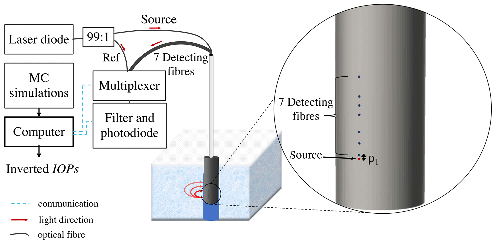
Figure 1 Experimental setup schematic. The 2 in. probe was designed to fit an auger hole drilled through the ice and to measure sideward on the edge of the hole. A laser diode emitted at $\mathit{\lambda }=\mathrm{633}\pm \mathrm{2}$ nm with a full width at half maximum of 1.4 nm and optical power of 300 mW. A 99:1 fibre optic coupler divided optical power between a leg used to guide light up to the probe head where injection into sea ice occurred and the reference leg. Detecting optical fibres at distances ρ₁₋₇ collected backscattered laser light (curved red arrows). An optical multiplexer selected the fibre to be read by a photodiode. A reflective bandpass filter centred at λ=633 nm with a full width at half maximum of 5 nm was placed before the photodiode to reject sunlight. A single-board computer with an easy-to-operate touch screen controlled the multiplexer, obtained Φ readings from the photodiode and did a field inversion on b.

The light source was a laser diode (PSU-III-DEL, Changchun New Industries™, Changchun, China) emitting a spectrum centred at a wavelength $\mathit{\lambda }=\mathrm{633}\pm \mathrm{2}$ nm with 1.4 nm full width at half maximum. The optical power of the laser was up to 300 mW at the tip of the emitting fibre with variations of less than 1 % after a warm-up of 5 min. A 99:1 fibre optic coupler (TM200R1S1A, Thorlabs™, Newton, United States) split optical power between the reference leg (∼1 % of power) and a leg used to guide light up to the probe head where injection into sea ice occurred (∼99 % of power). Seven optical fibres were positioned to collect backscattered laser light at source–detector distances ρ_1…7 of 2, 8, 14, 23, 28, 33 and 43 mm at the ice interface (see Fig. 2a). The printing allowed a precision of ±20 µm on fibre position. Source and detecting silica fibres (FT400UMT, Thorlabs™, Newton, United States) had a diameter of 400 µm and a NA of 0.41 at λ=633 nm (or Θ_det=18.3^∘ in ice). The measured Θ_source for the combination of laser, fibre optic coupler and source fibre was 7.3^∘ in ice. The source reference fibre and the detecting fibres were connected to an optical multiplexer (MPM-2000, Ocean Insight™, formerly Ocean Optics, Dunedin, United States) which selected the fibre to be measured. The output of the multiplexer was connected by the means of the same type of optical fibre to a photodiode (PH100-Si-HA-D0, Gentec-EO™, Quebec City, Canada). All detecting fibres, source reference fibre and a dark measurement were read by the photodiode in less than 30 s. A reflective bandpass filter centred at λ=633 nm with full width at half maximum of 5 nm was placed before the photodiode to reject sunlight at extraneous wavelengths. A single-board computer with a touch screen (Lattepanda DFR0444, DFRobot™, Shanghai, China) controlled the multiplexer and recorded the photodiode radiant flux Φ measurements. The touch screen and touch pencil allowed control of the instrument without taking out gloves, making operations under cold conditions more convenient.

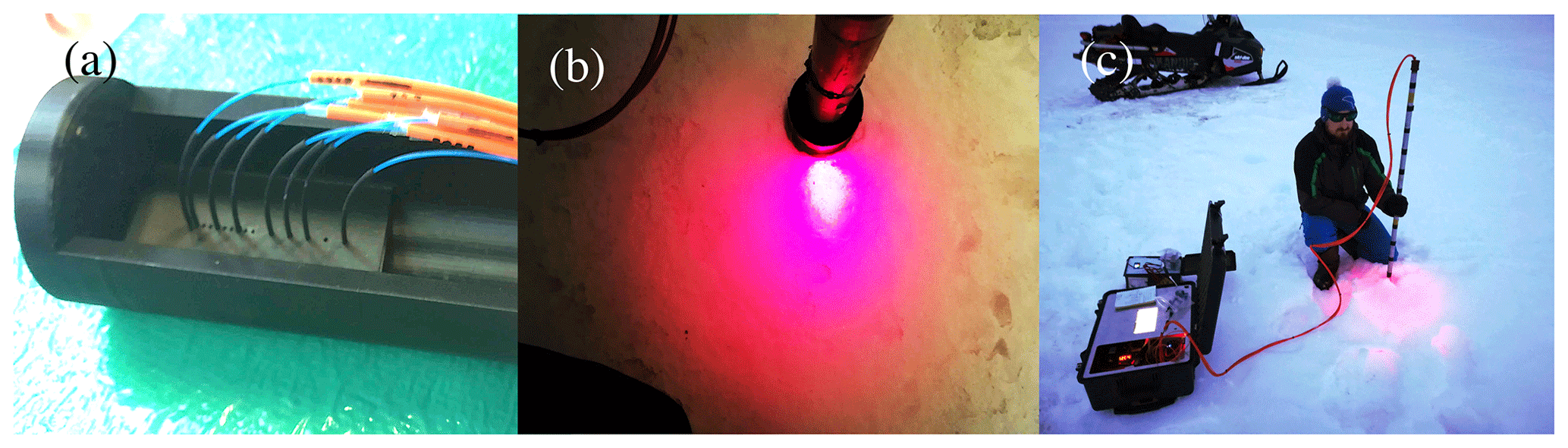
Figure 2 (a) Probe head interior. Source and detecting fibres were held in place with heat shrink tubes and glue. Fibres' bend radii are meant to respect the minimum long-term limit of 40 mm. (b) Probe head inserted in a 2 in. auger hole drilled in sea ice. (c) Probe operated on sea ice close to Qikiqtarjuaq Island on the coast of Baffin Bay.

The measured reflectance R_mes was calculated following

$$\begin{array}{}\text{(10)}& R_{\mathrm{mes},i}=c_i\cdot {\displaystyle \frac{{\mathrm{\Phi }}_i-{\mathrm{\Phi }}_{\mathrm{bg},i}}{\mathit{\eta }\cdot {\mathrm{\Phi }}_{\mathrm{ref}}}},\end{array}$$

where c is the calibration factor that accounts for the optical power losses through the system and the mismatch with Monte Carlo simulations. Φ_i is the backscattered radiant flux detected at the surface of the medium by fibre i, Φ_bg is the sum of the sunlight background radiant flux and dark noise, Φ_ref is the radiant flux detected by the source reference fibre, and η is the coupler split ratio ${\mathrm{\Phi }}_{\mathrm{source}}/{\mathrm{\Phi }}_{\mathrm{ref}}$.

3.2 Monte Carlo simulations for generation of the lookup table

Because we measure in the sub-diffusive regime, we cannot rely on an analytical solution to retrieve IOPs. Instead, we rely on a Monte Carlo numerical approach. We simulated the spatially resolved diffuse reflectance $R_{\mathrm{sim}}(\mathit{\rho },a,b,\mathit{\gamma })$ using the Monte Carlo software SimulO (Leymarie et al., 2010). The software allows creation of 3D environments with complex shapes, sources and detectors. It has been used and validated multiple times for research in ocean optics (e.g. Babin et al., 2012; Leymarie et al., 2010; Massicotte et al., 2018).

Figure 3 illustrates the numerical environment designed to simulate $R_{\mathrm{sim}}(\mathit{\rho },a,b,\mathit{\gamma })$ for our geometry. Light was emitted from the tip of the source fibre toward the probed medium. Photons were emitted in a direction inside Θ_source=7.26^∘ in ice. The emission angular profile of photons followed a Lambertian distribution. The medium representing sea ice was given a refractive index n_med, an absorption coefficient a, a scattering coefficient b and a phase function p(θ). We used the modified Henyey–Greenstein phase function p_mHG(θ) (see Eq. 7). Thus, g₁=βg_HG and $g_{\mathrm{2}}=\mathit{\beta }{g}_{\mathrm{HG}}^{\mathrm{2}}+\frac{\mathrm{2}}{\mathrm{5}}\left(\mathrm{1}-\mathit{\beta }\right)$ are defined accordingly. The environment overlaying the medium had a refractive index n_env. Two variations of the numerical environment were implemented. For measurement inside sea ice, the probed medium had the refractive index of ice (n_med=1.31) and the overlaying environment had the refractive index of water (n_env=1.33). For calibration and validation with solutions of microspheres, n_med=1.33 and n_env=1.

Figure 3 Schematic of the numerical environment used to simulate R_sim(ρab^′γ) with the Monte Carlo method.

Detecting fibres were replaced by a circular detector to collect photons over a larger area and, therefore, to reduce calculation time. It counted photons crossing with an incident half angle $\le {\mathrm{\Theta }}_{\det }=\mathrm{18.25}$^∘ in ice (NA=0.41). Photon counts were azimuthally averaged for 10 circular bins evenly distributed along the radius (ρ=0, 6.7, 13.3, 20.0, 26.7, 33.3, 40.0, 46.7, 53.3 and 60 mm) in order to cover the whole surface. The replacement of detecting fibres by a detector induced an error of less than 0.4 % on reflectance. The error came from Fresnel reflection on the tip of the detecting fibres which was not accounted for (Hecht and Zajac, 1974).

As explained in Sect. 2.2.2, the inverse procedure provides parameters a, $b=b\left(\mathrm{1}-g_{\mathrm{1}}\right)$ and $\mathit{\gamma }=\frac{\mathrm{1}-g_{\mathrm{2}}}{\mathrm{1}-g_{\mathrm{1}}}$. Thus, to facilitate a, b^′ and γ determination, we fixed g₁=0.98, a representative value for interior sea ice in situ (Mobley et al., 1998). We ran the simulations for 20 values of a from 0.01 to 3 m⁻¹, 92 values of b from 0.05 to 300 m⁻¹ and 7 values of γ from 0.8 to 1.98. Absorption and scattering properties were selected to cover sea ice IOPs as known from previous studies (Ehn et al., 2008a; Light et al., 2008, 2015; Mobley et al., 1998; Trodahl et al., 1987). The range of γ was limited by the mathematical condition on p_mHG(θ) where $\mathit{\beta }\in [\mathrm{0},\mathrm{1}]$ (see Eq. 7) (Bevilacqua and Depeursinge, 1999).

$R_{\mathrm{sim}}(\mathit{\rho },a,b,\mathit{\gamma })$ was simulated for every combination of a, b and γ with the numerical environment shown in Fig. 3. For every IOP combination, 10 simulations of 10⁶ photons were computed, and the normalized standard deviation $\mathit{\sigma }\left(R_{\mathrm{sim}}\right)/R_{\mathrm{sim}}$ between those simulations was obtained. $\mathit{\sigma }\left(R_{\mathrm{sim}}\right)/R_{\mathrm{sim}}$ was below 5 % when b≥2 m⁻¹ and was always less than 12 %. The large volume of calculation ($\mathrm{20}\times \mathrm{92}\times \mathrm{7}\times \mathrm{10}$ simulations of 10⁶ photons) required the use of Compute Canada computation resources. Even with high computation power, the 4D output matrix had an insufficient resolution to calculate precise IOPs. To increase resolution, we interpolated $R_{\mathrm{sim}}(\mathit{\rho },a,b,\mathit{\gamma })$ successively on a, b and γ dimensions with linear regression. Also, for the interpolated simulated spatially resolved diffuse reflectance ${\overline{R}}_{\mathrm{sim}}(\mathit{\rho },a,b,\mathit{\gamma })$ to match detecting fibre positions ρ_1…7, the matrix was linearly interpolated on the spatial dimension ρ. The final lookup table ${\overline{R}}_{\mathrm{sim}}({\mathit{\rho }}_{\mathrm{1}\mathrm{\dots }\mathrm{7}},a,b,\mathit{\gamma })$ was a $\mathrm{7}\times \mathrm{250}\times \mathrm{395}\times \mathrm{200}$ matrix. For visualization in the field, a lighter $\mathrm{7}\times \mathrm{1}\times \mathrm{395}\times \mathrm{1}$ matrix was implemented, fixing a to 0.22 m⁻¹ and γ to 1.98.

3.3 Inversion algorithm

Retrieval of a,b and γ was achieved by comparing R_mes(ρ₁₋₇) to every curve of an interpolated Monte Carlo simulated lookup table ${\overline{R}}_{\mathrm{sim}}({\mathit{\rho }}_{\mathrm{1}-\mathrm{7}},a,b,\mathit{\gamma })$. The error χ² for every variation of a,b and γ was calculated following

$$\begin{array}{}\text{(11)}& {\mathit{\chi }}^{\mathrm{2}}(a,b,\mathit{\gamma })=\sum _{i=\mathrm{1}}^{\mathrm{7}}{\displaystyle \frac{{\left(R_{\mathrm{mes}}\left({\mathit{\rho }}_i\right)-{\overline{R}}_{\mathrm{sim}}({\mathit{\rho }}_i,a,b^{\prime },\mathit{\gamma })\right)}^{\mathrm{2}}}{R_{\mathrm{mes}}\left({\mathit{\rho }}_i\right)}}.\end{array}$$

The simulation that fitted the best to the measurement was defined by the smallest element in the error matrix ${\mathit{\chi }}^{\mathrm{2}}(a,b,\mathit{\gamma })$. The coordinates a,b and γ of that element were the calculated IOPs (Fig. 4). Many versions of Eq. (11) were tested for robustness. Noticeably, the algorithm was less sensitive to noise when the subtraction was normalized by R_mes(ρ_i). Or said otherwise, the algorithm was less sensitive when the detecting fibres all had equal weights. The choice of a discrete interpolated matrix rather than a continuous method like Levenberg–Marquardt was motivated by robustness. Comparing measurements to every discrete element of ${\overline{R}}_{\mathrm{sim}}({\mathit{\rho }}_{\mathrm{1}-\mathrm{7}},a,b,\mathit{\gamma })$ insured we avoided incorrect inversion because of local minima in the error matrix. The downsides were heavier calculation time and larger memory needs.

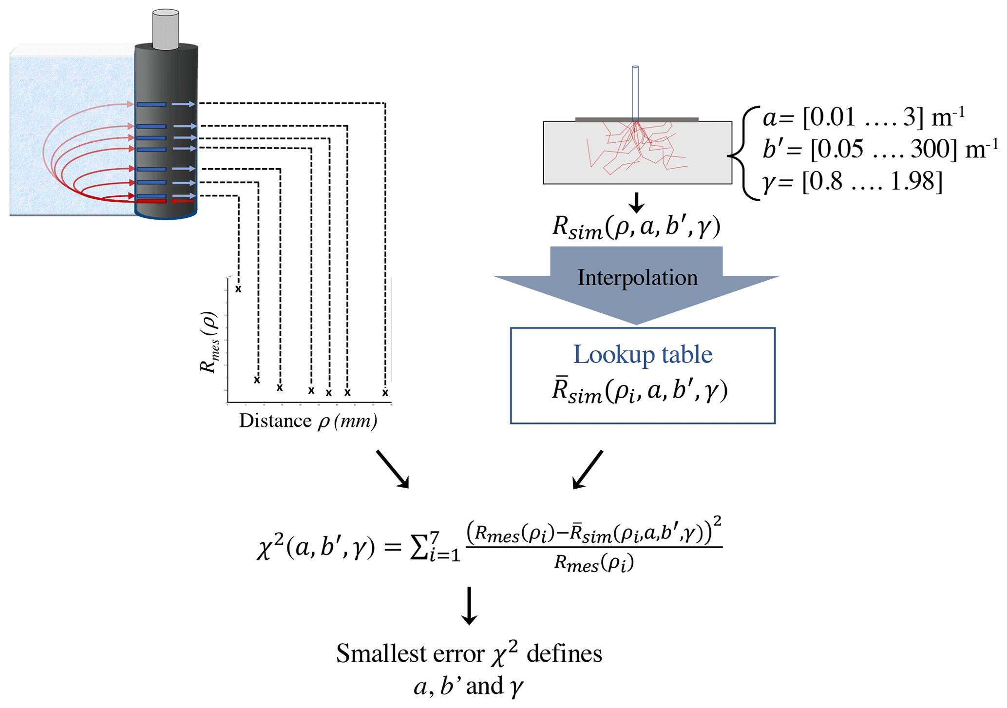
Figure 4 Illustration of the inversion algorithm used to retrieve inherent optical properties of sea ice.

3.4 Estimation of the depth of signal origin

The appropriate probed volume was evaluated based on two conditions. First, the signal of origin should reach deep enough to average the contribution of a large number of inclusions. Inclusions causing scattering in young sea ice (brine channels, air bubbles and precipitated salts) range from less than 1 µm up to rarely more than 10 mm (Light et al., 2003a; Perovich and Gow, 1991). Second, the depth of signal origin should be small enough to resolve the topmost and thinnest optical layer of sea ice, the surface scattering layer, with the probe leaned horizontally (meaning the fibres are looking downward). The surface scattering layer is typically no less than a couple of centimetres (Ehn et al., 2008a; Light et al., 2008, 2015). Based on these two criteria, we established that the ideal volume measured by the probe shall be deeper and wider than roughly 10 mm to encompass a large number of inclusions and, in the best scenario, shallower and narrower than 50 mm to resolve the optical properties of the surface scattering layer with the probe leaned horizontally looking downward.

Bevilacqua (1998) demonstrated that depth of signal origin is roughly proportional to ρ (for human tissues). Therefore, ρ tunes the probed volume. To verify the relation between ρ and the depth of signal origin for sea ice, which scatters and absorbs significantly less than human tissues, we ran Monte Carlo simulations. For this test, the numerical environment we used was similar to the environment shown in Fig. 3, except that a totally absorptive horizontal slab was inserted in the medium. The slab was lowered from the surface downward by increments Δz of 0.5 mm down to a depth z of 30 mm and by increments Δz of 4 mm deeper. The cumulative signal $R\left(z\mathit{\rho }\right)/R_{\max }\left(\mathit{\rho }\right)$ vs. absorptive plate depth z vs. ρ was evaluated for a=0.1 m⁻¹; b=10, 100 and 1000 m⁻¹; and g=0.94. We ran 40 simulations of 10⁶ photons for every z when b=10 and 100 m⁻¹ and 10 simulations of 10⁶ photons for every z when b=1000 m⁻¹. The standard deviation between simulations was used to evaluate the uncertainties. The depth, z₉₅, where $R\left(z\mathit{\rho }\right)/R_{\max }\left(\mathit{\rho }\right)$ is 95 % was linearly interpolated on the ρ dimension to obtain estimation at fibre positions ρ_1…7.

3.5 Calibration and validation using polystyrene microspheres in water

Prior to field tests, the probe was calibrated and IOP measurements were validated using reference media. Our reference media were suspensions of Polyscience™ polystyrene microspheres with a diameter of 1.93±0.01 µm in distilled water. The liquid medium was measured in a black container about 15 cm deep and 20 cm wide. Changing the microsphere volume fraction allowed us to tune a and b^′ of the medium. We obtained four reference points by a series of dilutions. The theoretical value of the absorption coefficient a was calculated by weighting water and polystyrene a values (Kadhim, 2016) by their respective volume fraction. The theoretical values of b^′ and γ were calculated using Mie theory (Bohren and Huffman, 1998). A magnetic stirrer ensured that the microsphere concentrations were homogeneous during measurements. We did not measure higher concentrations, resulting in higher a and b^′, because of the limitation in microsphere quantity.

To calibrate our system, the uncalibrated spatially resolved diffuse reflectance $R_{\mathrm{mes}}^{\ast }\left({\mathit{\rho }}_{\mathrm{1}\mathrm{\dots }\mathrm{7}}\right)$ measured from dilution no. 1 was compared to its closest corresponding simulation in ${\overline{R}}_{\mathrm{sim}}\left({\mathit{\rho }}_{\mathrm{1}\mathrm{\dots }\mathrm{7}}a{b}^{\prime }\mathit{\gamma }\right)$. The calibration factor c shown in Eq. (10) was calculated following

$$\begin{array}{}\text{(12)}& c_{\mathrm{1}\mathrm{\dots }\mathrm{7}}={\displaystyle \frac{{\overline{R}}_{\mathrm{sim}}\left({\mathit{\rho }}_{\mathrm{1}\mathrm{\dots }\mathrm{7}}\right)}{R_{\mathrm{mes}}^{\ast }\left({\mathit{\rho }}_{\mathrm{1}\mathrm{\dots }\mathrm{7}}\right)}}.\end{array}$$

The calibration factor accounted for the optical power losses through the system and the mismatch with simulations. The calibration factor c obtained on dilution no. 1 resulted in the lowest errors in the subsequent validation.

Table 1 Theoretically calculated IOPs for four concentrations of polystyrene microspheres in water used to first calibrate and then validate the instrument measurements.

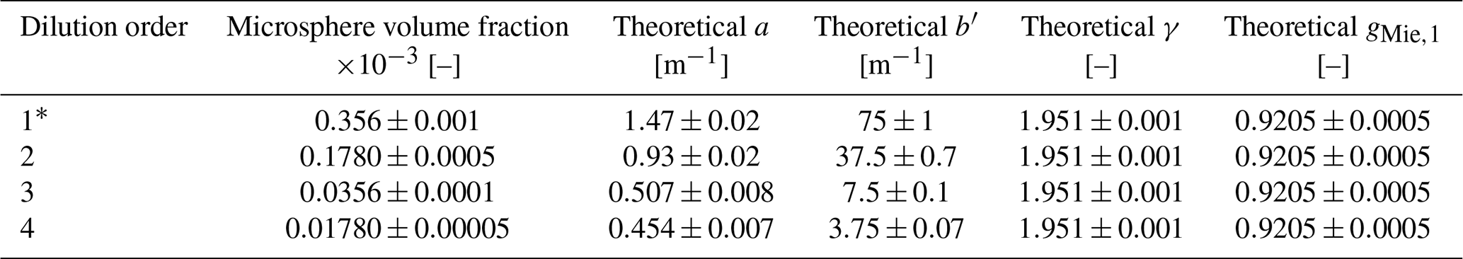
^∗ Used for calibration.

For validation, calibrated R_mes was entered in the inversion algorithm described in Sect. 3.3. Inversion algorithm and a, b^′ and γ were retrieved at all four concentrations. Measurements were taken 10 consecutive times. This way, we retrieved the mean and the standard deviation on a, b^′ and γ. The means were compared to theoretically calculated values. The instrument validation error e between measured IOPs and theoretically calculated IOPs is given by

$$\begin{array}{}\text{(13)}& e=\mathrm{100}\cdot {\displaystyle \frac{\left(\text{measurement}-\text{theoretical value}\right)}{\text{theoretical value}}}.\end{array}$$

3.6 Fieldwork

Using the spatially resolved diffuse reflectance method, we profiled first-year Arctic interior sea ice at two study sites around Qikiqtarjuaq Island next to Baffin Bay in Nunavut, Canada, from 7 to 10 May 2019 (Fig. 5). One site was on snow-covered ice (67.59^∘ N, 64.03^∘ W), and one site was on bare ice (no snow accumulation) (67.49^∘ N, 63.95^∘ W). Air temperature was between −6 and 3 ^∘C, and the sky was sunny with passing clouds for most of the sampling period. Both sites had a slightly positive freeboard. We were at the very beginning of the melt season and snow was starting to be slushy. A thin melt crust was present on snow at the snow-covered site. At the bottommost layer of the ice was a thin and pale algae layer. No other impurities were observed in the ice column.

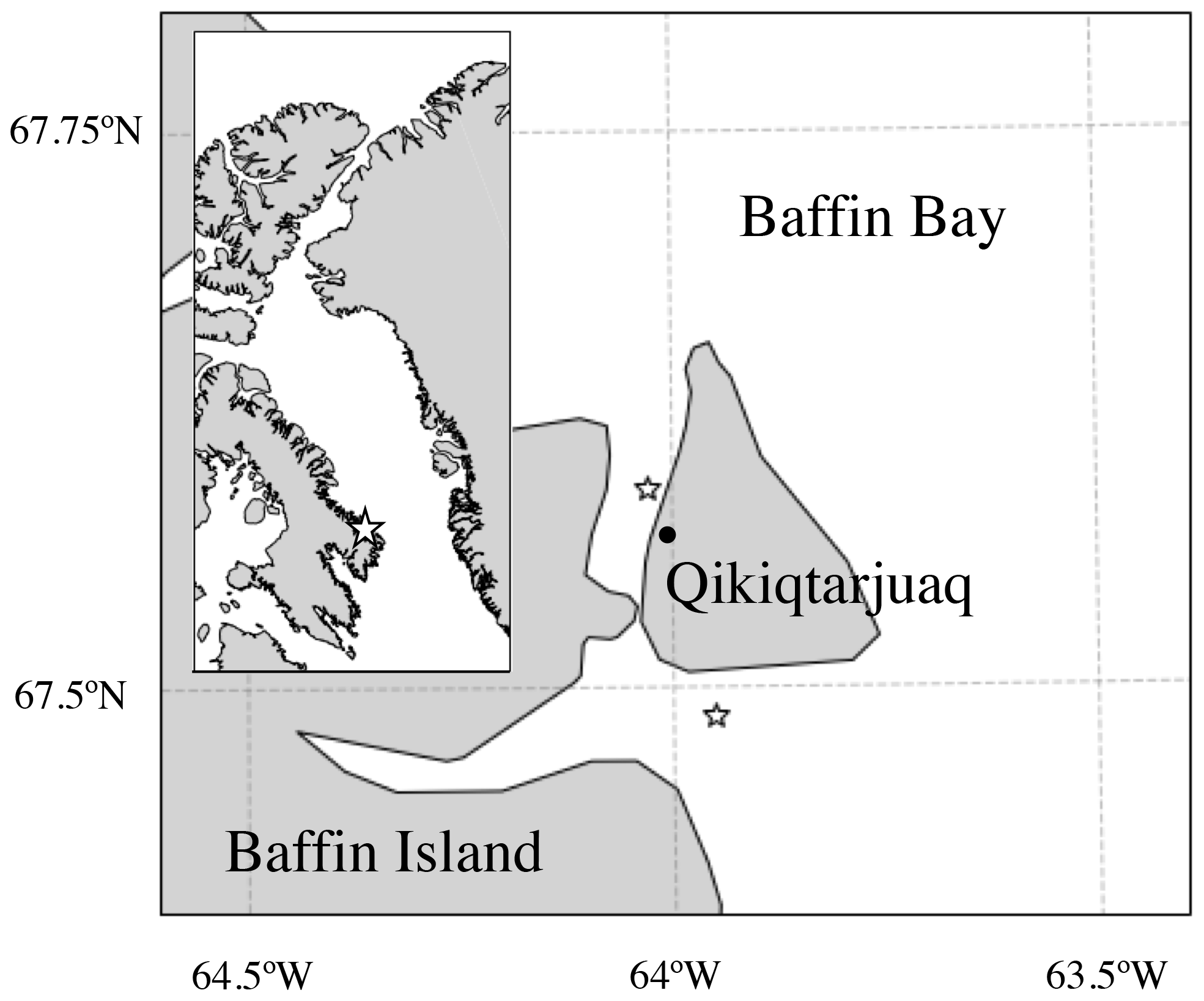
Figure 5 Locations of the snow-covered and bare-ice sampling sites visited on 8 and 9 May 2019 near Qikiqtarjuaq on the shore of Baffin Bay in Nunavut, Canada.

Sea ice thickness, snow thickness and freeboard were measured through the hole with a thickness gauge (Kovacs Entreprises™, Roseburg, United States).

After a warm-up of 5 min, the probe head was inserted inside a 2 in. auger hole (Fig. 2b–c). Emission reference flux Φ_ref and Φ₁₋₇ were measured every 10 cm starting from the top and lowering the probe head until the bottom of the hole. When the bottom was reached, the laser was shut down. Then, sunlight background Φ_bg was measured with the probe at every depth on the way up. Field trials have shown that the sunlight background is significant as it can have the same order of magnitude as the signal in the worst scenario (and is 10⁴ times smaller in the best scenario). For every depth, R_mes(ρ_1…7) was obtained (see Eq. 10), and b was inverted from it with fixed a and γ. The output result is a profile of b vs. depth in the ice. Measurements were repeated in the same hole with a tent, with a tarpaulin covering the ground (at bare-ice site only) and with no cover to shield sunlight. The use of a tent or of a tarpaulin diminishes the sunlight background by roughly 1 and 2 orders of magnitude respectively.

After profiling, an ice core was retrieved next to the sampling site using an ice corer (Mark II 0.09 m diameter 1 m long corer, Kovacs Entreprises™, Roseburg, United States). A picture of the ice core was obtained for qualitative observation of the ice scattering properties. Ice temperature T was measured at the centre of the core at 10 cm intervals using a high-precision thermometer (VWR International™, Radnor, United States – ±0.1 ^∘C). For the measurement of bulk salinity S, the core was cut in 10 cm sections. Ice sections were melted in plastic bags. The S of the melted ice section was measured using a conductometer (738-ISM, Mettler-Toledo InLab™, Columbus, United States).

4 Results

4.1 Depth of signal origin

Figure 6 shows $R\left(zr\right)/R_{\max }\left(\mathit{\rho }\right)$ vs. absorptive plate depth z at different ρ. The depth of signal origin was dependent on the scattering properties of the medium. When scattering was low (b=10 m⁻¹), as for interior ice, z₉₅ was 110±20 mm when detecting at ρ₂=8 mm and was 270±20 mm when detecting at ρ₆=43 mm. When scattering was high (b=1000 m⁻¹), as for surface scattering ice, z₉₅ was 39±2 mm when detecting at ρ₂ and was 78±4 mm when detecting at ρ₆.

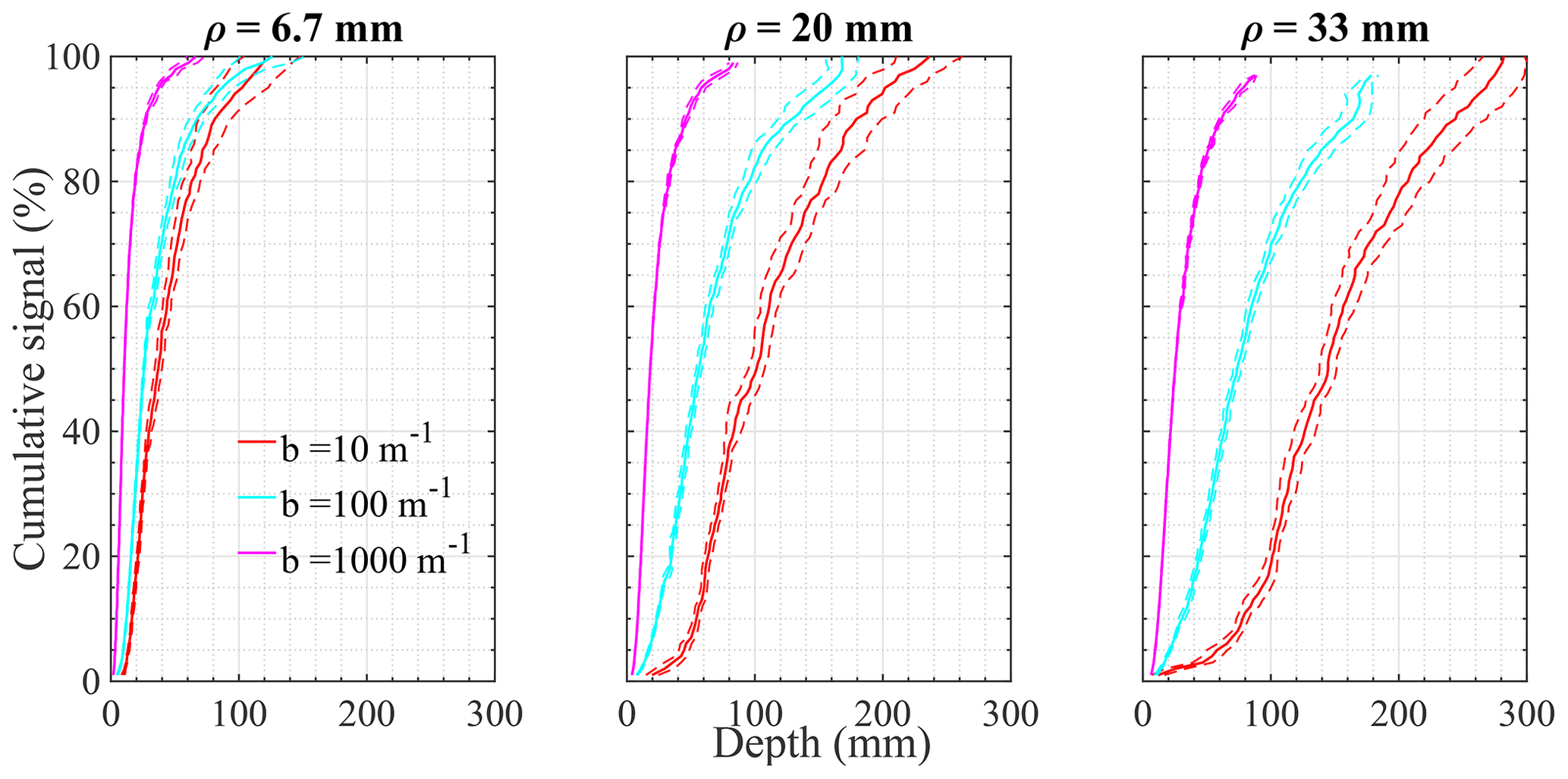
Figure 6 Estimation of the depth of signal origin for our probe geometry simulated by Monte Carlo. The cumulative signal $R\left(zr\right)/R_{z\max }\left(r\right)$ vs. absorptive plate depth z at different lateral distances ρ was evaluated for three b values typical of sea ice, a=0.1 m⁻¹ and g=0.94. We ran 40 simulations of 10⁶ photons for every z when b=10 and 100 m⁻¹ and 10 simulations of 10⁶ photons for every z when b=1000 m⁻¹. The standard deviation on simulations was used to evaluate uncertainties.

No matter ρ_i and b, z₉₅ was always significantly greater than our minimum criterion of 10 mm (see Sect. 3.4), suggesting the signal originates from sufficiently deep to encompass even large scattering inclusions. In highly scattering ice, fibres ρ_4…7 had a z₉₅ greater than our maximum criterion of 50 mm. It implies that scanning the surface scattering layer with the probe leaning horizontally (looking downward) on the surface is not always possible. In that case, detecting fibres ρ_i should be carefully chosen so that their signal of origin is shallower than the scattering layer depth. Since we did not measure surface scattering layer properties in the case of this study, we did not further consider this maximum criterion.

4.2 Validation

Figure 7 compares the mean a, b^′ and γ to the theoretical values for four concentrations of microspheres in distilled water as reference media. a and b theoretical values covered close to 2 orders of magnitude and were typical of sea ice. The Mie phase function was forward peaked as for sea ice. The e on measured IOPs is defined by Eq. (13). Fibres 1 and 7 were taken out of the inversion because fibre at ρ₁=2 mm was very close to the source and never met the criterion where $\mathrm{0.5}\le \mathit{\rho }{b}^{\prime }$ needed to be in the N=2 regime (see Sect. 2.2.2), and fibre at ρ₇=43 mm had a calibration factor c₇ roughly 10 times greater than calibration factors c₁₋₆. Either the simulated reflectance ${\overline{R}}_{\mathrm{sim}}$ was not correctly modelled at this distance or fibre 7 was damaged.

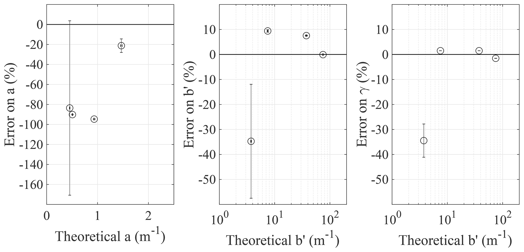
Figure 7 Validation of IOP measurements using reference media. The reference media were four solutions of polystyrene microspheres in distilled water. Microsphere concentrations were chosen for the theoretical a and b^′ ranges to cover sea ice typical values. Detecting fibres 1 and 7 were taken out for optimized results.

Using fibres 2 to 6, we obtained |e| between 21 % and 94 % for a, between 0.06 % and 35 % for b^′, and between 1.5 % and 34 % for γ. These values are comparable to those obtained with classical instruments in marine optics (Leymarie et al., 2010). Standard deviations on e were fairly low except at the lowest concentration where the inverted IOPs were very sensitive to signal variation. There, we obtained standard deviations of 87 % on a, 23 % on b^′ and 7 % on γ. For this specific concentration, the depth z₉₅ is potentially greater than the depth of the container (∼15 cm) for fibres at distances ρ₃₋₆ (see Sect. 4.1). The absorptive effect of the bottom container wall could explain the substantially higher value and uncertainty of e at this concentration. All higher concentrations result in a z₉₅ significantly smaller than the depth of the container no matter ρ, and therefore their value should not be affected by the bottom wall. Uncertainties on theoretically calculated IOPs came from the uncertainty on the microspheres' mean diameter. For the three parameters, the uncertainties were less than 2 %.

4.3 Physical properties of the sampled sea ice

The first site was covered with 24 cm of snow. The ice thickness was 104 cm with a 2 cm freeboard. The second site was uncovered (bare ice), therefore allowing more growth and thicker ice. The ice thickness was 135 cm with a 3 cm freeboard. Ice cores were taken out roughly 5 m away from optical measurement holes. Observations were made at the beginning of the melt season when snow was starting to be slushy. A thin melt crust was present on snow at the snow-covered site.

Figure 8a shows T vertical profiles. At the snow-covered site, the lowest temperature was at the surface and was close to −4 ^∘C. Temperature rose progressively and reached over −2 ^∘C at the bottom. At the bare-ice site, the temperature profile was c-shaped. The temperature at the surface was over −2^∘C, and the minimum was reached at 65 cm and was close to −4 ^∘C. The temperature rose back to over −2^∘C at the bottom. The upper surface was warmer at the bare-ice site because of the direct heat transfer from air.

Figure 8b shows S vertical profiles. At the snow-covered site, the bulk salinity profile was c-shaped. The bulk salinity at the surface was 6.6 ‰. This value was high enough to suggest the uppermost boundary was formed of sea ice only. The minimum was reached at 65 cm and was 3.4 ‰. Bulk salinity rose back to over 7.2 ‰ at the bottom. At the bare-ice site, the uppermost section had a bulk salinity of 2.7 ‰, which suggests brine drainage by gravity and melting. The bulk salinity stayed close to 5 ‰ through the ice core and rose to 7.7 ‰ at the bottom section.

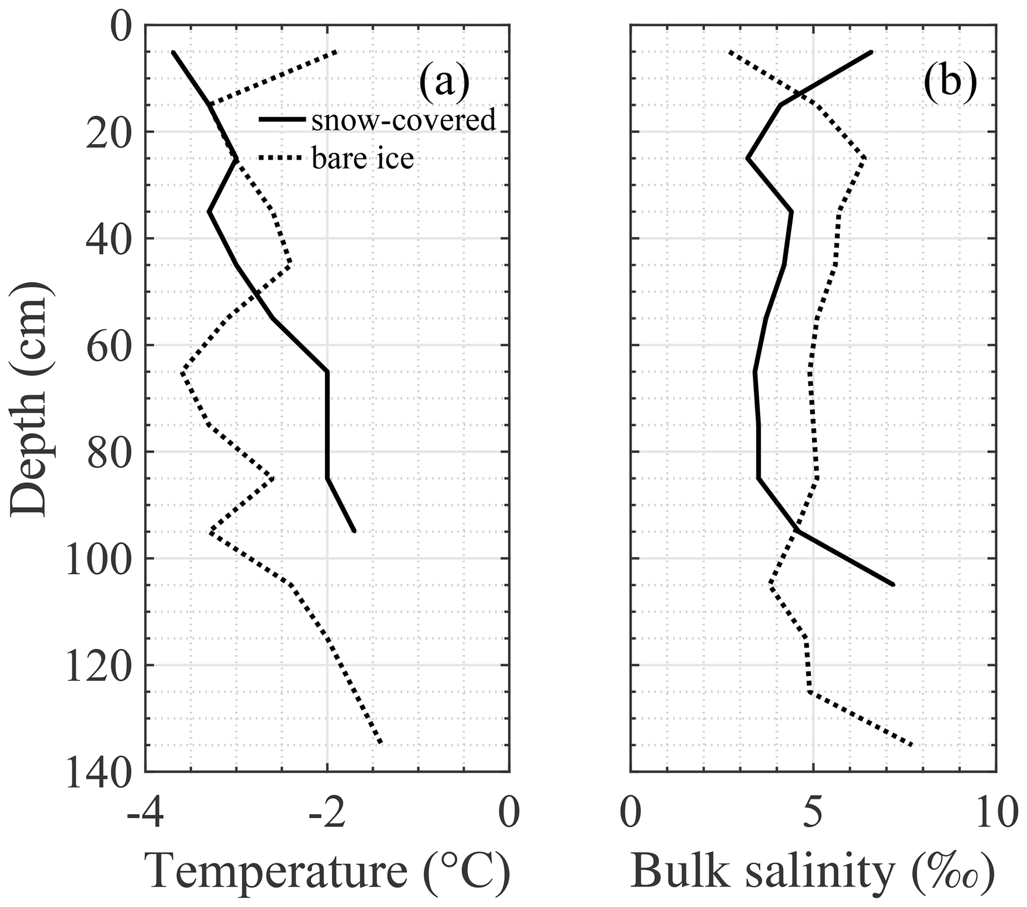
Figure 8 Profiles of (a) T and (b) S measured on ice cores nearby optical measurement holes at both sites.

4.4 Vertical profiles of b with fixed a and γ

At both sites, vertical profiles of b were acquired with the probe in a 2 in. auger hole with a and γ fixed. The motivation to fix a and γ was to reduce their influence on inverted b; we fixed a to 0.22 m⁻¹ because e was close to −100 % on the range corresponding to pure sea ice at λ=633 nm (see Fig. 7). The value we chose corresponds to pure ice at λ=633 nm (Picard et al., 2016). Also, we fixed γ to 1.98 when scanning sea ice and to 1.86 when scanning snow because γ measurements in the ice were highly noisy. These values were obtained assuming g₁ was 0.98 and 0.86 respectively and assuming the phase function followed a Henyey–Greenstein distribution ($g_{\mathrm{2}}=g_{\mathrm{1}}^{\mathrm{2}})$. These values and distribution are commonly used to represent p(θ) of sea ice in larger-scale radiative transfer calculations (Grenfell, 1983). Finally, b^′ measurements were not considered if R_mes and ${\overline{R}}_{\mathrm{sim}}$ were off by more than 40 % for either fibre 2 or 3. This criterion was the best we found to take out false inversion results.

Measurements of b were acquired every 10 cm from the snow or ice surface until we reached the bottom (Fig. 9). Measurements were repeated at the same location with and without a tent covering the measurement hole to limit incident sunlight. At the bare-ice site, a profile with a 3×3 m tarpaulin fixed to the ground as a sunshade was also obtained. The same profiles with and without subtraction of sunlight background Φ_bg from R_mes were compared (see Eq. 10).

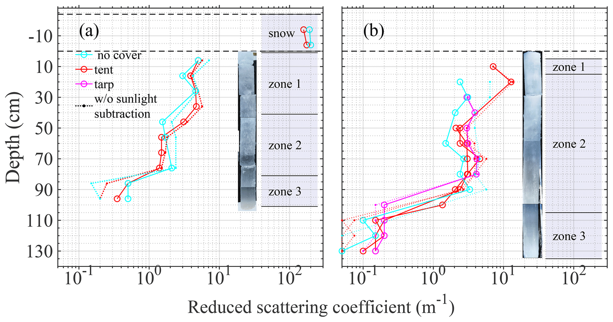
Figure 9 Reduced scattering coefficient b^′ vs. depth measured actively in situ inside first-year Arctic interior sea ice. Measurements were taken (a) at a snow-covered site and (b) at a bare-ice site. Pictures show ice cores extracted a few metres away from the sampling holes. The profiles were separated by zones at depth where we observed significant changes in the value of b^′. We compared measurements using different covers to shade from sunlight. We also compared with and without subtracting the residual sunlight background flux Φ_bg.

For both sampling sites, we observed a decrease in the value of b from the top to the bottom of the ice. We divided the profile into zones at depths where the b values changed significantly. Here, the uncertainties represent the standard deviation for every measurement within the given depth interval. At the snow-covered site, we observed four different zones. The average b for snow was 160±10 m⁻¹, the average b for depths between 6 and 36 cm was 4.4±0.7 m⁻¹, the average b for depths between 46 and 76 cm was 2.1±0.8 m⁻¹, and the average b for depths between 86 and 96 cm was 0.46±0.07 m⁻¹. At the bare-ice site, we observed three different zones. The b value at a depth of 10 cm was 7.1 m⁻¹. The average b for depths between 20 and 100 cm was 2.8±0.8 m⁻¹. For this zone, two measurements at the boundaries were discarded. One of those two was taken at a depth of 20 cm and had a value of 12.8 m⁻¹, which is much greater than the standard deviation. We believe the measurement was taken slightly closer to the surface and would have been more representative of the first zone of ice. The other measurement taken at a depth of 100 cm was 0.2 m⁻¹. We think the measurement was taken slightly deeper and therefore was included in the third zone. The average b for depths between 110 and 130 cm was 0.15±0.05 m⁻¹. It is believed that the variability in the measurements was the consequence of heterogeneity in the ice morphology.

Ice core photographs from both sites showed a change in colour from whitish to translucid, which was consistent with b vertical decay. At the snow-covered site, the transition from zone 1 to zone 2 at a depth of 46 cm was barely apparent on the picture. It corresponded to a drop of the mean b from 4.4±0.7 m⁻¹ to 2.1±0.8 m⁻¹. This was expected since the measurements of the two zones almost overlapped. The transition from zone 2 to zone 3 was easily distinguished in the picture. It corresponded to a drop of the mean b from 2.1±0.8 m⁻¹ to 0.46±0.07 m⁻¹. This was a 5-fold drop. However, the transition occurred 6 to 16 cm shallower in the picture. The ice cores were retrieved approximately 5 m away from the optical measurement sites. Therefore, the spatial variation in the ice structure might explain the imperfect depth consistency between b vertical profiles and the picture.

The three pictures stitched together were taken at different angles, and therefore sunlight reflection gave the false impression of a transition in the ice. This effect was more obvious at the bare-ice site, which made the comparison to the picture too difficult.

5 Discussion

5.1 Sensitivity of b to a and γ

The inverted b values depend on the choice of fixed a and γ values. Thus, we analyzed the sensitivity of b to these two parameters for the profiles presented in Fig. 9. Varying fixed a from 0.01 to 0.5 m⁻¹ induced no significant variation on b profiles except in the very-low-scattering ice of zone 3 where it induced variations of up to 50 %. However, for every zone, varying fixed γ from 0.8 to 1.98 induced very significant variations of up to an order of magnitude on inverted b.

Our choice of fixed γ=1.98 is the value representing Henyey–Greenstein p(θ) with g₁=0.98 (thus g₂=0.98²) (see Eq. 9). This choice is commonly used for larger-scale radiative transfer in interior sea ice (Grenfell, 1983), where only g₁ is relevant. Better insight into the in situ p(θ) of sea ice would be needed to say whether the Henyey–Greenstein distribution realistically represents its moments g₂₊. Indeed, the knowledge of the g₂ range in sea ice could be used to restrain γ to a smaller, more plausible range, reducing the uncertainty on b.

But even then, the sensitivity to g₃₊ in low-scattering ice would still remain a source of uncertainty. Since inverting on three parameters (a, b and γ) is already challenging, it is inconceivable to add higher phase function similarity parameters to account for the dependency on g₃₊ in the inversion. Not to mention that barely more useful structural information would be carried by these higher-similarity parameters. If g₃₊ values are relatively stable in sea ice, one could simply find a p(θ) modelling g₃₊ of sea ice accurately for calculation of the lookup table. If g₃₊ values are variable in sea ice, one could replace γ by a phase function similarity parameter, like the σ parameter introduced by Bodenschatz et al. (2016), which combines the contribution of every phase function moment g_n.

5.2 Comparison to previous measurement methods

Figure 10 compares the vertical average of b obtained for both sampling sites to the vertical averages of b measured in the past on polar interior sea ice using different methods (see Sect. 2.2). Trodahl et al. (1987) and Mobley et al. (1998) reported a single value, while Light et al. (2008, 2015) reported ranges that represent a seasonal evolution. For Ehn et al. (2008a), the range represents different ice types. Average b values for the different zones are also shown to illustrate the variability within interior sea ice. The error bars on our measurements represent the standard deviation for all b measurements in the given depth interval.

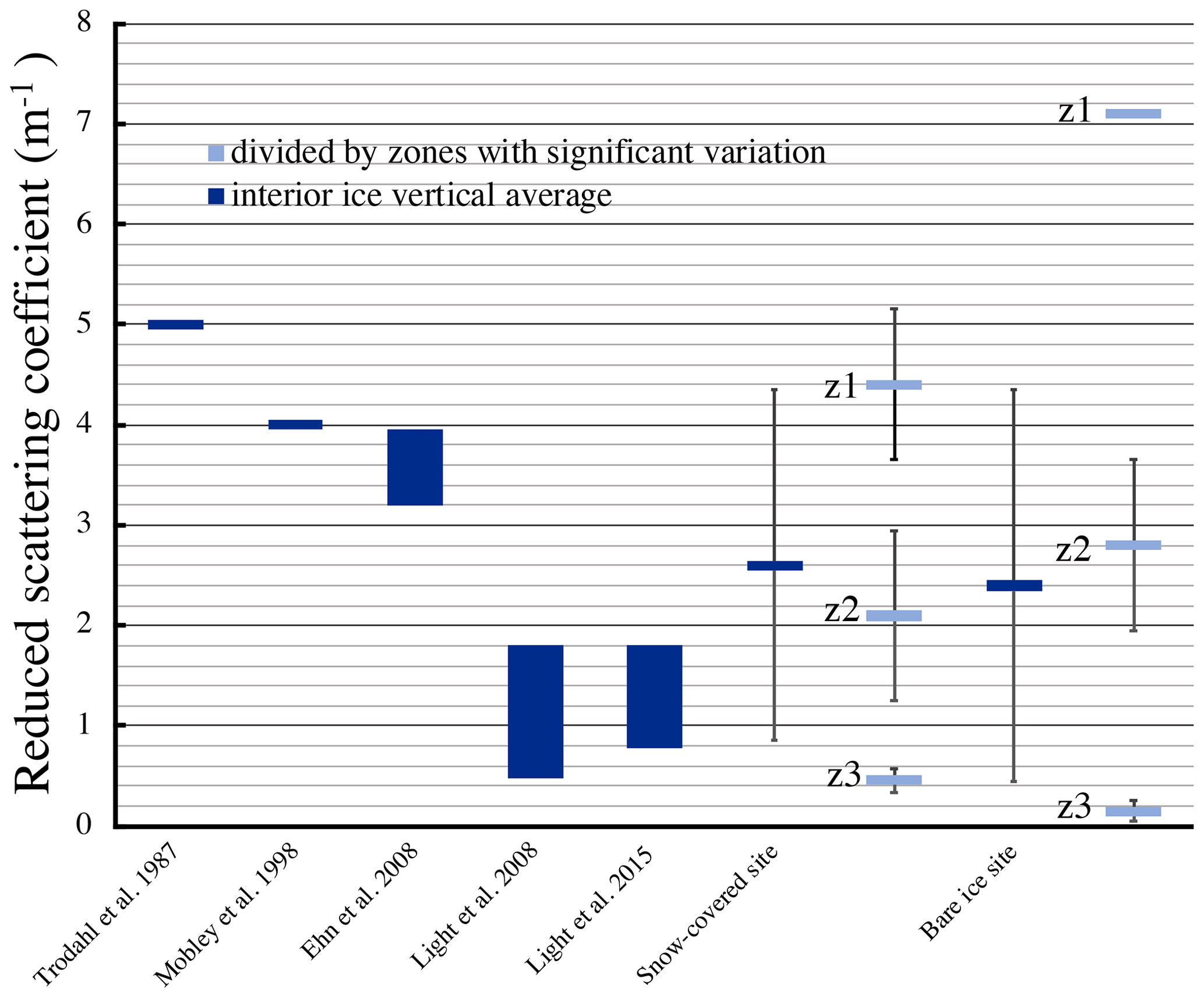
Figure 10 Comparison of the vertical averages of b measured in situ at both sampling sites to vertical averages of b published over the past for polar interior sea ice using various methods. For our measurements, the average reduced scattering coefficient b is also divided by zones. Zones are separated at depths where we observed significant changes in scattering properties. The error bars represent the standard deviation for the given depth interval.

For our fieldwork, the vertical average of b was 2.6±1.7 m⁻¹ for the snow-covered site and was 2.4±1.9 m⁻¹ for the bare-ice site. These values are comparable to vertical averages of b measured by other authors. They are smaller than Trodahl et al. (1987), Mobley et al. (1998) and Ehn et al. (2008a), but greater than Light et al. (2008, 2015).

Our method was sufficiently resolved to observe the transitions in the optical properties of the interior ice in situ, demonstrating a strong vertical variability. Indeed, the standard deviations on the vertical average of b represented 65 % and 80 % of the mean. Furthermore, for both samples, average b of the uppermost zone was an order of magnitude greater than average b of the bottommost zone. This high vertical variability in the properties of interior sea ice highlights the necessity of a vertically resolved in situ technique like spatially resolved diffuse reflectance, allowing the division of the vertical profile into smaller, more homogeneous zones. Vertically divided b could then be more easily associated with a set of physical measurements (e.g. appearance, temperature, salinity, porosity, inclusion size and shape distributions) particular to the given zone.

5.3 Comparison to ice core images

Table 2 shows b measurements together with ice core pictures for the three zones we identified at the snow-covered site. Our pictures focused on the central depth of the zones in order to avoid ambiguities. These were compared to the b measurements and pictures of drained ice and interior ice by Light et al. (2008). No optical measurements were taken the day the core was photographed (17 July). Thus we define the upper and lower limits of b^′ to be the closest measurement dates (9 and 21 July).

Table 2 Average b measurements together with ice core pictures for the three zones we identified at the snow-covered site compared to the b measurements and pictures of drained ice and interior ice adapted from Light et al. (2008).

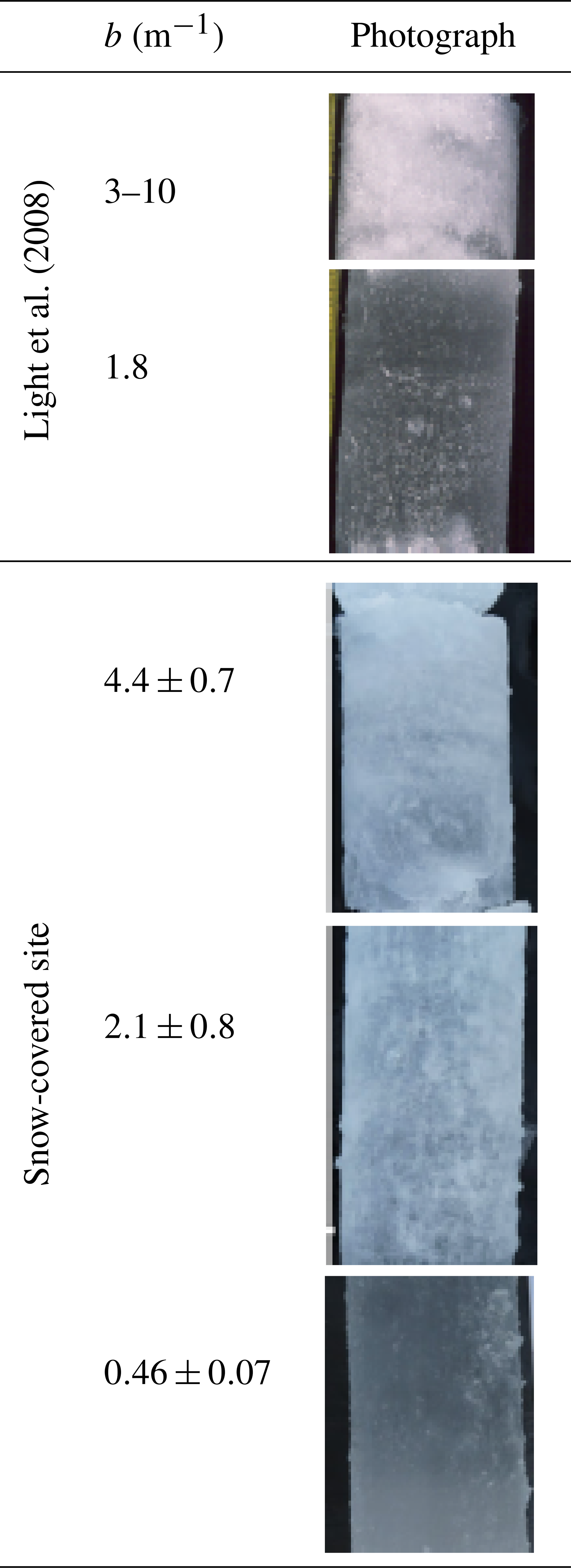
The drained ice sample of Light et al. (2008) was distinctively whiter than the samples of zones 1 and 2 of our ice core. The b range associated with the drained ice sample overlaps the range of zone 1. However, the value of b^′ associated with the drained ice core photograph is probably closer to 10 m⁻¹, being closer in time to the upper limit. The interior ice sample of Light et al. (2008) showed a similar appearance to the ice of zone 3, yet with more white heterogeneities. Again, this goes along with the b measurement being greater than our value. The comparison of b measurements and ice core pictures is consistent with Light et al. (2008), which suggests our measurements to be in the right range.

5.4 Comparison to structural-optical model

Using the Grenfell (1983) framework, Light et al. (2003a, 2004) established a structural-optical model to determine b of an ice sample in a laboratory for T starting from −30 to 0 ^∘C (see Sect. 2.2). This b vs. T relationship was established for a salinity S of 4.7 ‰, which is close to what we measured. We compared our T profiles (see Fig. 8a) to their relationship in order to retrieve b. At both sites, the estimated vertical average of b was 8.8±0.1 m⁻¹. It should be kept in mind that keeping S constant to 4.7 ‰ reduced the variability of estimated b.

These values were roughly 3.5 times greater than what we measured in situ with the reflectance probe. We suppose this is because the laboratory model was corrected for brine channel drainage occurring when extracting the core from the ice. Channel drainage augments the refractive index difference between the channel and the ice, which augments scattering efficiency and affects the phase function. Change of gas volume and merging inclusions might also affect scattering differently in the laboratory.

The extension of the structural-optical model to obtain in situ estimation of the IOPs is a difficult task, in particular because estimation of b requires knowledge of the distributions of sizes and shapes of the scattering inclusions in sea ice. Over the past, these distributions were estimated by means of microscope observations in a cold laboratory (Light et al., 2003a). Combining vertically resolved in situ b measurements to laboratory structure observations could potentially bridge that difficulty. Indeed, the structural-optical framework could be tuned to meet in situ b measurements the same way it is tuned to meet laboratory active b measurements in Light et al. (2004). For example, brine channel drainage, scattering by hydrohalite salts, the brine channel merging, and air bubble merging and escaping could be adjusted to meet in situ conditions. The estimation of in situ b based on the temperature, bulk salinity, and size and shape distributions of the scattering inclusions of sea ice would be an interesting breakthrough. Indeed, it opens the door to the empirical estimation of in situ b based on sea ice growth conditions.

5.5 Error analysis

5.5.1 Estimation of error in sea ice based on validation

To estimate the error made on b when measuring inside sea ice, we compared in situ measurements to the instrument validation measurements made on microsphere solutions. The b validation points closest to our given b measurement inside ice established the boundaries of the corresponding error. Table 3 summarizes the instrument validation error e attributed to the average of b of the different ice zones. For this analysis to make sense, we assumed that e was the lowest at its calibration point ($b^{\prime }=\mathrm{75}\pm \mathrm{1}$ m⁻¹) and that e diverged as we moved away from this point.

Table 3 Summary of mean b for the different ice and snow zones of both sampling sites and the corresponding instrument validation error e. Zones were separated at depth where we observed significant changes in b. The corresponding e was based on the validation with microsphere solutions.

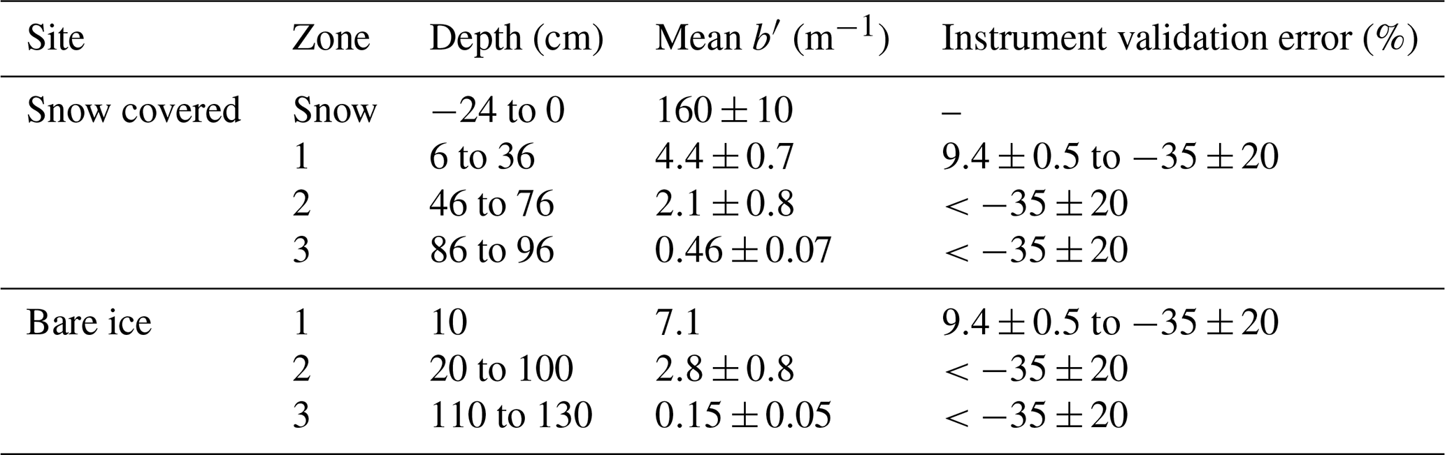
For both sites, zone 1 had a e between −35 % and 9.4 %, and zones 2 and 3 had e below −35 %. Because the b^′ values in zone 2 were close to the validation point at $b^{\prime }=\mathrm{3.75}\pm \mathrm{0.07}$ m⁻¹, we assumed that $e=-\mathrm{35}$ % was a decent estimation. The b^′ values in zone 3 were far from the closest validation point. Therefore, e on these values was probably greater than −35 %. Because scattering for this zone was very low, we assumed that its influence on radiative transfer was also low. We can therefore tolerate higher e for this zone.

The e attributed to the different ice zones might be overestimated, especially because we measured in low-scattering ice. During validation with microsphere solutions, the measurement of b was altered by the depth of the container (15 cm). For low-scattering medium (b=10 m⁻¹), roughly no signal was cut for the first measuring fibres, but up to 20 % of the signal originated from deeper than the container at fibre 4 and 45 % at fibre 6 (see Fig. 6). Because R_mes was cut, inverted b was underestimated compared to the theoretical value, which might explain higher error e.

The e could also be high because IOP measurement in low-scattering media is intrinsically difficult. As mentioned in Sect. 2.2.2, we assumed in our model that a phase function with two moments was sufficient to model reflectance. However, in media with low-scattering ice properties, we do not meet the minimum criterion on the optical distance $\mathit{\rho }{b}^{\prime }>\mathrm{0.5}$ mandatory for this assumption to be true. Not considering the moments of the phase function greater than 2 is therefore likely to lead to the underestimation of b in the validation.

5.5.2 Additional errors induced when measuring inside sea ice

We must keep in mind that this estimation of the measurement error inside sea ice is by no means absolute as there are key differences between measurements inside sea ice and measurements on the microsphere solutions used for validation. While a and γ are free in the validation, they are fixed when measuring inside sea ice. As mentioned in Sect. 5.1, the inversion of γ can have a significant effect on the inversion of b^′.

Also, the sunlight background is not negligible and represents an additional source of error when measuring inside sea ice. Field trials have shown that it can have the same order of magnitude as the signal in the worst scenario and be 10⁴ times smaller in the best scenario. Even though the sunlight background radiant flux Φ_bg is measured on the way up after profiling and subtracted from R_mes, it left a noise on the measurements nevertheless. This is the reason why we obtained different b profiles depending on the sun shading method (see Fig. 9).

6 Conclusion

We developed and validated a method to measure vertically resolved in situ inherent optical properties (IOPs) of sea ice. Conceptually, the spatially resolved diffuse reflectance R_mes(ρ) measured from the ice interface is compared to a Monte Carlo simulated lookup table. The inversion algorithm inverts the absorption coefficient a, the reduced scattering coefficient b and the phase function parameter γ of a constrained volume (∼ dm³). Monte Carlo simulations showed that the depth cumulating 95 % of the signal z₉₅ is between 40±2 and 270±20 mm depending on the source–detector distance ρ and on the ice scattering properties. Validation of the measurements with microsphere solutions showed that the magnitude of the instrument validation error |e| was between 21 % and 94 % for a, between 0.07 % and 35 % for b^′, and between 1.5 % and 34 % for γ. The |e| on b^′ measurements was evaluated over close to 2 orders of magnitude corresponding to values typical of low- and medium-scattering sea ice.

We tested the probe on first-year Arctic interior sea ice at two study sites around Qikiqtarjuaq Island next to Baffin Bay in Nunavut, Canada from 7 to 10 May 2019, at the very beginning of the melt season. In the light of validation results, we fixed a to 0.22 m⁻¹ and γ to 1.98 and focused on the dominant and easier-to-retrieve b. We measured every 10 cm sideward on the edge of an auger hole drilled through the ice. At the snow-covered site, we obtained b of 4.4±0.7 m⁻¹ for the uppermost zone of interior ice and b of 0.46±0.07 m⁻¹ for the bottommost zone. At the bare-ice site, we obtained a single b measurement of 7.1 m⁻¹ for the uppermost zone of interior ice and b of 0.15±0.05 m⁻¹ for the bottommost zone. These b measurements are sensitive to the choice of γ, revealing the need for a better representation of the higher moments of the in situ phase function of sea ice. Our results emphasize the strong vertical variability of the scattering properties even within interior sea ice. These values are in the range of polar interior sea ice mean b measurements previously published with different methods by other authors. We demonstrated that the magnitude of b was consistent with the appearance of the ice core at the snow-covered site.

We believe combining vertically resolved in situ b measurements with laboratory structure observations could help to bridge structural and optical knowledge of sea ice. Indeed, the structural-optical framework of Grenfell (1983) could be tuned to meet in situ b measurements the same way it was tuned to meet laboratory active b measurements in Light et al. (2004). Combining in situ and laboratory observations could open the door to empirical radiative transfer estimations based on sea ice growth conditions. We believe that further developments of the spatially resolved diffuse reflectance method will lead toward more widespread and wide-ranging studies and an improved comprehension of in situ IOPs of sea ice.