the Creative Commons Attribution 4.0 License.
the Creative Commons Attribution 4.0 License.
 | 07 Sep 2021
Southern Ocean polynyas in CMIP6 models
Céline Heuzé
Sebastiaan Swart
Polynyas facilitate air–sea fluxes, impacting climate-relevant properties such as sea ice formation and deep water production. Despite their importance, polynyas have been poorly represented in past generations of climate models. Here we present a method to track the presence, frequency and spatial distribution of polynyas in the Southern Ocean in 27 models participating in the Climate Model Intercomparison Project Phase 6 (CMIP6) and two satellite-based sea ice products. Only half of the 27 models form open-water polynyas (OWPs), and most underestimate their area. As in satellite observations, three models show episodes of high OWP activity separated by decades of no OWP, while other models unrealistically create OWPs nearly every year. In contrast, the coastal polynya area is overestimated in most models, with the least accurate representations occurring in the models with the coarsest horizontal resolution. We show that the presence or absence of OWPs is linked to changes in the regional hydrography, specifically the linkages between polynya activity with deep water convection and/or the shoaling of the upper water column thermocline. Models with an accurate Antarctic Circumpolar Current transport and wind stress curl have too frequent OWPs. Biases in polynya representation continue to exist in climate models, which has an impact on the regional ocean circulation and ventilation that should be addressed. However, emerging iceberg discharge schemes, more adequate vertical grid type or overflow parameterisation are anticipated to improve polynya representations and associated climate prediction in the future.
- Article
(14481 KB) - Full-text XML
- BibTeX
- EndNote


Polynyas are areas of open water surrounded by sea ice. They are common features within the Southern Ocean winter sea ice and are often classified into two different categories: coastal polynyas and open-water polynyas (OWPs). Coastal polynyas are usually latent heat polynyas that are kept open by winds that drive the sea ice away from the coastline or an obstacle, like an iceberg (Morales Maqueda et al., 2004). OWPs are kept open by thermodynamic processes, such as upwelling of sensible heat or diffusive fluxes (Martinson and Iannuzzi, 1998) that transport warm water masses upwards, melting the sea ice and keeping the regional ocean ice-free. The heat source that keeps OWPs from freezing over is the presence of comparatively warm and salty Circumpolar Deep Water (CDW), which is usually located just below the base of the upper mixed layer (Santoso et al., 2006). These warmer waters transport heat from the depth to the surface by free or forced convection, caused by surface cooling, brine rejection, or wind and shear stresses respectively (Williams et al., 2007). While open-ocean deep convection is closely linked to OWPs (Cheon and Gordon, 2019), deep convection is not a sufficient condition for OWPs to occur (Dufour et al., 2017).
Polynyas play a key role in sea ice and deep water formation. In winter, the strong temperature contrast between the open water in the polynyas and the cold Antarctic air causes significant heat loss of several hundred W m−2 from the ocean to the atmosphere (Willmott et al., 2007). In fact, while the area of coastal polynyas is only about 1 % of the sea ice area in the Southern Ocean, 10 % of Antarctic sea ice is produced there owing to this intense cooling (Tamura et al., 2008). The rapid ice production in coastal polynyas also produces a water mass of extremely high density, the Dense Shelf Water. This water is considered to be the main source of Antarctic Bottom Water, which forms the deepest layer of the global oceans (Orsi et al., 1999).
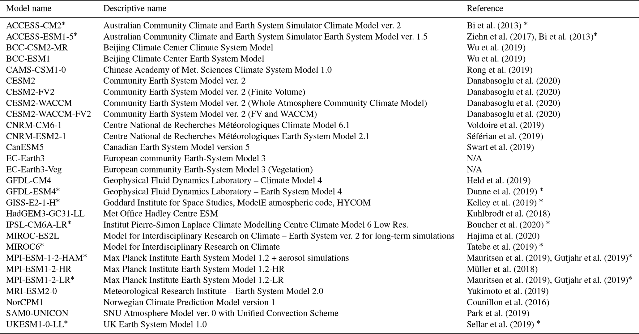
Table 1The 27 CMIP6 models used in this study. Columns show the model names, ocean component, nominal horizontal resolution of the ocean (Ro [km]), atmosphere component, horizontal resolution of the atmosphere (Ra [km]), sea ice component, vertical discretisation scheme including number of vertical levels (z: depth level, ρ: isopycnal, σ: terrain-following, several symbols: hybrid grid), data availability of monthly sea ice concentration (Cm), daily sea ice concentration (Cd), monthly sea ice thickness (Tm) and daily sea ice floe thickness (FTd).

Some coastal polynyas open at the same location every year (e.g. the Ross Sea polynya), while OWPs are observed only once per decade or less. The Weddell Sea polynya has been the largest OWP observed to date and affected the water properties in the Weddell Sea for decades (Zanowski et al., 2015). It was first observed in the winters of 1974–1976, with an average area of up to 300 000 km2 (Carsey, 1980); produced about 5 Sv of Antarctic Bottom Water (Wang et al, 2017); and led to a significant cooling at mid-depth (Cheon and Gordon, 2019). Only minor polynyas have been observed in the region from 1976 to 2016 (Cheon and Gordon, 2019), when the Maud Rise polynya (Swart et al., 2018; Heuzé et al., 2019; Francis et al., 2019) reached an area larger than 50 000 km2, similar to the polynya of October–November 1973 (Cheon and Gordon, 2019). These Weddell Sea and Maud Rise polynyas were preceded by a phase of positive Southern Annular Mode (SAM) anomalies and strong Southern Hemisphere westerlies (Gordon et al., 2007; Campbell et al., 2019; Cheon et al., 2014). Behrens et al. (2016) found that deep convection, as it happens in OWPs, is strengthening the meridional density gradients and increases the Antarctic Circumpolar Current (ACC) transport on multidecadal timescales.
Polynya detection in observational data (e.g. Markus and Burns, 1995; Kern et al., 2007; Ohshima et al., 2016) and ocean reanalysis products (Aguiar et al., 2017) and the role of OWPs in spurious deep water formation in CMIP5 (Heuzé, 2015) have been discussed before. The formation of OWPs in models has been shown to be very sensitive to vertical mixing parameters (e.g. Kjellsson et al., 2015; Heuzé, 2015), initial sea ice conditions (e.g. Kjellsson et al., 2015), stratification (e.g. De Lavergne et al., 2014; Stoessel et al., 2015) and model resolution (e.g. Dufour et al., 2017; Kurtakoti et al., 2018; Lockwood et al., 2021). A weak background stability, especially in the Weddell Sea (Wilson et al., 2019), makes the ocean susceptible to convective overturning due to model inaccuracies such as a lack of dense shelf water overflows (Dufour et al., 2017) or heat buildup due to insufficient vertical mixing (Heuzé et al., 2015). Spurious OWP appearance or deep convection in the Weddell Sea remains a challenge in modern climate models (e.g. Held et al., 2019; Sellar et al., 2019; Mauritsen et al., 2019; and references marked with an asterisk (*) in Table A1). Ocean convection due to static instabilities is an important process in the formation of OWPs, which is not modelled directly due to the relatively coarse resolution of many CMIP6 models (Table 1) but parameterised instead (e.g. Hasumi, 2000; Madec et al., 2017). Despite the crucial role of OWPs for sea ice production and deep water properties, an evaluation and comparison of their representation across current climate models is missing.
Here we determine the characteristics, causes and impacts of Southern Ocean polynyas in 27 models that participated in the Climate Model Intercomparison Project Phase 6 (CMIP6, Eyring et al., 2016). We present a new method to detect polynyas from daily and monthly sea ice concentration or thickness in CMIP6 models and observational data sets in Sect. 3. We use this approach to assess Southern Ocean polynya characteristics (spatial distribution, frequency and seasonality) for the entire CMIP6 historical run, check whether major issues documented in earlier CMIP versions still remain and compare the modelled polynyas with observational satellite data when available in Sect. 4. As observational data from within OWPs are very sparse, we continue with a comparison of the models' hydrography in sea-ice-covered conditions to that occurring during OWP events in order to assess OWPs' impact on the entire water column. Finally, with the obtained polynya statistics from the CMIP6 models, we determine whether the observed correlations between the SAM, Southern Hemisphere westerlies, ACC transport, and the presence or magnitude of OWPs hold true across CMIP6 models (Sect. 5). We first consider the entire Southern Ocean south of 55∘ S and then focus on the Weddell Sea region, between 65∘ W and 30∘ E.
We start with a description of the analysed data and then present the algorithm that we use in Sect. 3 to find polynyas. We used for this study two remote observation-based sea ice products for sea ice concentration and thickness that we introduce in Sects. 2.2 and 2.3, as well as the sea ice output from the historical run of 27 CMIP6 models (Eyring et al., 2016, listed in Table 1).
2.1 Choice of CMIP6 models
We created a subset of all available CMIP6 models by filtering for models that participate in the historical CMIP6 scenario, have at least one sea ice variable downloadable in a monthly or daily format, and provide adequate projection and cell area information. The historical CMIP6 run covers the years from 1 January 1850 to 31 December 2014 and is forced with observed historical greenhouse gas concentrations. As of the latest date of download (October 2020), only one ensemble member was available for the majority of models. Consequently, we chose one representative ensemble member (r1i1p1f2 for CNRM models, r1i1p1f3 for HadGEM and r1i1p1f1 otherwise) for each model. This way, we ensure consistency with other CMIP sea ice area evaluations (Roach et al., 2020; Turner et al., 2013). In the 27 analysed models, the nominal horizontal resolution varies between 0.25 and 1.5∘ for the ocean (including the sea ice) and between 1 and 2.5∘ for the atmosphere (Table 1). All computations were performed on the models' native grid unless specified otherwise. The grid cell area (“areacello”) was used to compute the surface area of sea ice and polynyas. The models were purposely not detrended, as we want to determine the accuracy of their historical run with ongoing climate change incorporated into the analysis. For the assessment of polynya activity in the Southern Ocean, we use the sea ice concentration and sea ice thickness as discussed below.
2.2 Sea ice concentration
Sea ice concentration (CMIP6 parameter: “siconc”) is available at a daily resolution for only 18 of the 27 models, whereas it is available at a monthly resolution for all 27 models (Table 1). Furthermore, the daily sea ice concentration is not available for the full historical period for the models MRI-ESM2-0 (1 January 1920–31 December 2015) and SAM0-UNICON (1 January 1950–31 December 2015). Routine satellite-based sea ice concentration observations are available from January 1979 onwards, so there are 35 years of overlap with the historical CMIP6 model run on which we can perform our comparisons. We use the daily satellite-observation-based Global Sea Ice Concentration climate data record (OSI-450) (Lavergne et al., 2019) for the time period 1979–2015. For the time after 2015, an extension with the name OSI-430-b is available that is processed with the same algorithms (Lavergne et al., 2019). OSI-450/430b are sea ice concentration products, computed from SMMR (1979–1987), SSM/I (1987–2008), and SSMIS (2006–2020) microwave radiometers and ECMWF ERA-Interim reanalysis data (Dee et al., 2011). They are provided at a 25 km × 25 km horizontal resolution and daily temporal resolution from 1 January 1979 to 2020 onwards (every other day until 1985). The uncertainty in sea ice concentration is less than 4 % on average (Lavergne et al., 2019).
Using sea ice concentration to detect polynya activity has the advantage that it is available for the largest number of CMIP6 models (Table 1) and has been observed by satellite for more than 40 years. The disadvantage is that sea ice concentration is a poor choice to detect coastal polynyas that are often covered by newly forming thin sea ice in winter, and their full extent is better characterised by a low sea ice thickness (Ohshima et al., 2016). Polynya detection by sea ice thickness thresholds is well established (e.g. Ohshima et al., 2016; Nakata et al., 2015; Kern et al., 2007) and detects even polynyas that are covered by a thin layer of newly formed sea ice. Due to the described advantages and disadvantages of using either sea ice concentration (“siconc”) or thickness (“sivol”), we have decided, where practical, to analyse both and present the resulting data side by side in Sects. 3 and 4.
2.3 Sea ice thickness
For the CMIP models, two output variables related to the sea ice thickness are available. The sea ice volume per grid cell area (sivol) has been available in earlier CMIP versions and is commonly and hereafter referred to as equivalent sea ice thickness or just thickness. With CMIP6, a new sea ice variable called ice floe thickness (“sithick”) is introduced and available for the majority of models (Table 1). The equivalent sea ice thickness sivol is available for 23 of the models, but only at a monthly averaged resolution. Polynyas are dynamic processes and can change their area and position drastically within few days (Nakata et al., 2015; Kern et al., 2007); thus it is optimal to analyse daily data from all data sources if available. The ice floe thickness sithick is available on a daily resolution for 21 of our models, but we found it poor for our polynya detection, as we show in Sect. 3.3.
For observational comparison of the sea ice thickness, we use the daily, satellite-based Soil Moisture and Ocean Salinity (SMOS) thin sea ice thickness product (Huntemann et al., 2014). The product consists of maps of sea ice thickness up to 0.5 m, derived from the satellite-borne L-band radiometer SMOS. The data are distributed at a horizontal resolution of 12.5 km × 12.5 km and available from 1 June 2010 onwards. The sea ice thickness calculation from satellite data is a relatively new method that works best for ice thickness values of up to 50 cm, with an average retrieval error of about 30 % of the retrieved value (Huntemann et al., 2014). It does not take differences in sea ice concentration into account and might thus be biased in regions with low sea ice concentration. The accuracy of the method is negatively affected by melt ponds (ponds that form on the sea ice in the melting season), but low air humidity causes melt ponds to occur much less frequently on the Antarctic sea ice compared to the Arctic sea ice (Andreas and Ackley, 1982). The thin sea ice retrieval is a method that is more established for Arctic regions (e.g. Tietsche et al., 2018), but papers about its quality and applicability for the Southern Ocean are in preparation (e.g. Mchedlishvili et al., 2021). Even though the 10-year time period is too short for deriving climatological mean values, we decided to include it as an observational baseline, where relevant, to compare the CMIP6 data to.
2.4 Vertical ocean profiles
We do not limit our analysis to the surface of the ocean but also analyse vertical ocean profiles within CMIP6 polynyas. The majority of models use a z-level vertical grid in the ocean, with the exceptions of GFDL-CM4/ESM4, MIROC6/ES2L and NorCPM1. The GFDL models use isopycnal coordinates in the interior ocean and rescale to geopotential vertical coordinates in the mixed layer. The MIROC6 model uses hybrid z–σ coordinates between the sea surface and a fixed geopotential depth and a z-level grid below. NorCPM1 uses isopycnal coordinates in the interior ocean and z coordinates in the mixed layer; it is also the only model using data assimilation (Counillon et al., 2016). To investigate the hydrography we extracted vertical profiles from the monthly ocean salinity (“so”) and potential temperature (“thetao”). For observational comparison of the water properties, data from a SOCCOM vertical profiling float (Johnson et al., 2018) are used. We use temperature and salinity profiles measured by the SOCCOM float 5904471, because it provides a long record of profiles including rare vertical profiles from within the 2017 Maud Rise OWP (Campbell et al., 2019).
In this work, we present a new method to detect and distinguish coastal and OWPs using either sea ice concentration or equivalent sea ice thickness (Fig. 1). We apply this method to the observational, satellite-based products and the CMIP6 models listed in Table 1.
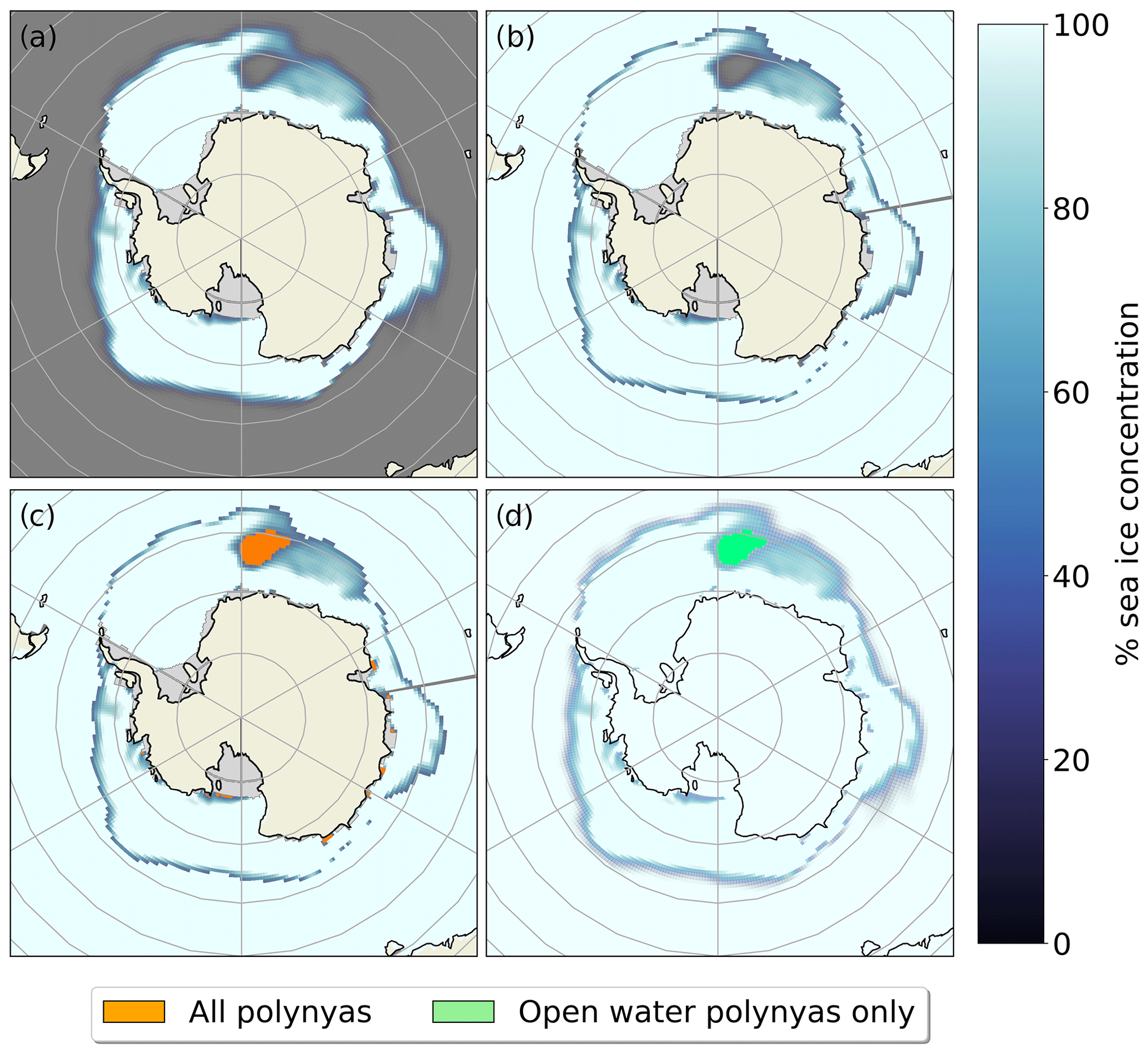
Figure 1A four-step algorithm classifies surface type areas in the marginal ice zone. (a) August 2002 monthly mean sea ice concentration from ACCESS-ESM1.5. (b) Sea ice map after covering the open ocean with the flood fill algorithm. (c) Application of a threshold filter, highlighting the total polynya areas. (d) Flood fill algorithm is applied to Antarctic fast land; the remaining open water or low sea ice areas are classified OWPs. The ice shelves appear in light grey and the ocean in dark grey.

Figure 2Illustration of the effect of different sea ice concentration thresholds on the detection of polynyas. (a) Observational sea ice concentration (OSI450) from 25 November 2017. (b) Combined area of coastal polynyas (orange) and OWPs (green) for sea ice concentration thresholds from 0 % to 100 %. The vertical lines correspond to the results of our algorithm for (c) 15 %, (d) 30 % and (e) 60 % sea ice threshold.
3.1 Our algorithm to detect polynyas
With the aim of detecting polynyas, we start with the sea ice concentration or thickness (Fig. 1a). To mask out the open ocean beyond the northern sea ice extent, we use a “flood fill” algorithm from the scikit-image library (Van der Walt et al., 2014). Starting from a grid cell with no sea ice, the seed, the algorithm detects similar cells below a specified sea ice concentration/thickness and masks them out, effectively “filling them” with ice (Fig. 1b). Afterwards, a maximum sea ice threshold filter returns all grid cells that are classified as “polynyas” (Fig. 1c). To differentiate coastal polynyas from OWPs, in a third step the flood fill algorithm is applied to the Antarctic continent (Fig. 1d). The Antarctic continent and ice shelves are represented by zero sea ice concentration/thickness in most models; for the exceptions that mark these grid cells in another way (e.g. infinite or negative value), we map this values to zero first. Coastal polynyas, adjacent to the land or ice shelves, are hence also covered by the flood fill algorithm. The grid cells below the threshold that remain are classified as “OWP”. The polynya area is the sum of the grid cell areas. The obtained OWP areas can be subtracted from the total polynya area to obtain the coastal polynya areas.
Depending on the chosen threshold and sea ice variable, the resulting polynya and sea ice areas differ. For example a closed layer of thin sea ice will be detected as a polynya if using the threshold thickness criteria but not if using the threshold sea ice concentration (siconc) criteria; an area with relatively sparse but thick sea ice will be classified as a polynya by the threshold sea ice concentration (siconc) criteria but not if using the threshold sea ice thickness (sivol) criteria. In the literature, a wide range of values for the concentration thresholds are in use. Previous studies on polynyas tend to choose a high sea ice concentration threshold to maximise the number of polynyas detected (e.g. Arbetter et al., 2004; Gordon et al., 2007), while sea-ice-specific studies choose a low threshold to capture all areas with sea ice. For example, Shu et al. (2015) and Beadling et al. (2020) use a 15 % threshold to estimate the sea ice extent in CMIP5 and CMIP6 models, Kern et al. (2007) classify areas with up to 45 % sea ice coverage as open-water areas, and Smedsrud (2005) points out that sea ice coverages of 80 %–90 % already allow for significant heat exchange and can therefore be classified as polynyas. The influence of different sea ice thresholds on our four-step algorithm is visualised in Fig. 2: the areas that are classified as polynyas increase with higher sea ice concentration thresholds, until the first polynya areas merge with the open ocean and thus become embayments (Fig. 2b, e). High sea ice concentration thresholds (up to ∼ 85 %) maximise the number of detectable coastal polynyas but lead to poor detection of OWPs (Fig. 2e). The higher the chosen sea ice threshold, the lower the area that is classified as sea ice. We found that almost no coastal polynyas are detected at a 15 % threshold in our observational product (Fig. 2b, c) and in most CMIP6 models (not shown). Therefore, we chose a 30 % sea ice concentration threshold as a good compromise: higher thresholds lead to a strong negative bias in sea ice area compared to other papers, and polynyas can become embayments as shown in Fig. 2e; lower values leave too many polynyas undetected. For thresholds higher than 60 %, the OWP area is increasing again (Fig. 2b) after the big OWP in the Weddell Sea merged with the open ocean. However, this signal is relatively noisy in time (not shown) and sensitive to small threshold changes (Fig. 2b). While more and more polynyas become embayments, new areas with more than 60 % sea ice concentration are classified as “polynyas”, and the area classified as “sea ice covered” in between shrinks. For the sea ice thickness threshold, we chose a value of 12 cm. This is consistent with Nakata et al. (2015), who give the total polynya extent as the areas occupied by open water and thin ice (up to 12 cm). For a discussion of the effect of different sea ice thickness thresholds, see Nakata et al. (2015) and Kern et al. (2007).
Some CMIP6 models provide only monthly averaged data, others include the sea ice concentration at daily resolution (Table 1). It is obvious that monthly data are unsuitable to detect a phenomenon that may last but a few days and that consequently the usage of monthly averaged sea ice output may affect the accuracy of the mean polynya areas. When comparing the daily observational data to monthly model output, we computed the monthly time mean of the sea ice concentration and thickness first and applied our algorithm then. To provide yearly averaged winter polynya area for each model and observational product, we used yearly polynya area averages:
In Eq. (1), Ad(t) and Am(t) are the polynya areas derived from 1 d or 1 month. Ndays and Nmonths are the total number of days or months in the time series. As we show in Sect. 4.2, coastal polynyas grow very large in the summer season, but we focus on winter polynyas here due to their large importance in ocean–atmosphere heat exchange and sea ice formation. We used the results from Eq. (1) to create scatter plots with least squares linear regressions (Figs. A1 and A2). For the observational sea ice concentration, the slope of the regression fit is 0.73, indicating that total polynya areas are underestimated by 27 % if computed from monthly averages and should be derived from daily data wherever possible. The regression is worst with OWP, probably because of the small number of OWPs in the observational data (Fig. A1). Seven of 18 CMIP6 models have a regression slope higher than or equal to the observational product (ACCESS-CM2, BCC-CSM2-MR, CNRM-CM6-1, CNRM-ESM2-1, EC-Earth3(-Veg), MPI-ESM1-2-HR), i.e. a better agreement between daily and monthly polynya areas, while the rest have a lower slope. We find a higher correlation for models including larger polynyas (total polynya area km2) compared to models that have only minor polynyas. We suspect that smaller polynyas have a shorter average life span and are more prone to relative changes in area due to ice drift.
The correlation of yearly polynya areas from equivalent sea ice thickness (sivol) with sea ice concentration (siconc) shows a slope of 0.31 for the observational data sets SMOS thin ice and OSI-450/430 (Fig. A2). Here we could only use the common time period from 2010 to 2020. The low slope indicates that our algorithm classifies 69 % less area as polynya when using sea ice concentration. This is not necessarily an erratic underestimation in this case but rather originates in different definitions of a polynya either using a concentration or thickness threshold. However, for 12 of the 23 models this slope is higher, indicating a closer relationship between low sea ice thickness and concentration. This is likely due to the conceptual differences between the observational sea ice thickness and the CMIP6 sea ice thickness. The observational sea ice thickness retrieval algorithm assumes sea ice concentrations of 100 % (Huntemann et al., 2014), while the sea ice thickness variable we use for our analysis is an area-averaged sea ice thickness and is thus directly connected to changes in sea ice concentration. We found low slopes in models with more coastal polynyas (e.g. MRI-ESM2.0: 0.00, IPSL-CM6A: 0.05, CESM2: 0.11) but also in the BCC models that form wide areas of thin sea ice (<10 cm) followed by a thicker ring along the outer sea ice edge (not shown).
3.2 Averaging methods
For readability, we condensed the data further in several ways depending on the objective of the analysis. To analyse the spatial distribution of polynyas, we present sea ice maps for September with polynya occurrences highlighted (Figs. 3, A3, A4). We chose the month of September as it typically features the austral sea ice maximum and is therefore discussed in related CMIP6 sea ice and Southern Ocean evaluations (e.g. Beadling et al., 2020; Roach et al., 2020). However, we also give the different seasonality of the modelled coastal and OWPs in Sect. 4.2. In Figs. 6, 7, A1, and A2 and for the polynya areas in Table 2, we used Eq. (1) first and took the mean over all model years then. For the sea ice extent in Table 2 and the maximum polynya extents in Fig. 6, we used
for daily and monthly variables respectively. For the figures within this paper we present the result of the analysis of either the sea ice concentration or thickness in either daily or monthly resolution to keep the data comparable. Not all plots include all 27 analysed models, since some models do not provide all output variables (Table 1). To avoid unnecessary repetitions in the paper, we do not always present the results from all sea ice variables used but keep some results exclusive to the Appendix figures.
In Sect. 4, we limit the analysis to the period May to November in order to filter out summer polynyas. Throughout the paper, we use the mean yearly polynya area for the winter season if not specified otherwise. In sea ice melting summer conditions, polynyas often become very large, but we want to focus on winter polynyas due to their importance in heat exchange and ice and deep water formation. Moreover, it is not recommended to use the SMOS thin ice product during melting season (Huntemann et al., 2014). When comparing model output data to the observational sea ice concentrations, we further limit the yearly mean values to a common time period from 1979–2015 to ensure consistency.
3.3 Sea ice floe thickness
The sea ice floe thickness (sithick) is defined as the actual thickness of the sea ice in the CMIP6 models, averaged over the ice-covered part of the grid cell (Huntemann et al., 2014). While the detected polynya locations and areas in our analysis of the sea ice concentration and thickness (Figs. 3, A3, A4) agree reasonably well with observations for most models and will be discussed further, we could not achieve satisfactory results if using only the sea ice floe thickness as input data (Fig. 4). The majority of the models (e.g. ACCESS, BCCs, CESM2s, MPIs, IPSL-CM6A-LR, MRI-ESM2-0, SAM0-UNICON) included increasing sea ice floe thickness beyond the outer sea ice extent of the concentration maps. These models also have a considerable mean floe thickness inside areas that would be classified as polynyas by low sea ice concentration and equivalent thickness (e.g. Fig. 4j, k). When using our thickness threshold algorithm with this data set, we obtain large OWPs in areas that hardly correspond to the observations (Fig. 4a–i), because the high ice floe thickness anomalies at the outer sea ice edges encircle large areas with thinner ice floe thickness.
A combined approach in which either low sea ice concentration or thickness or the product of both classifies an area as polynya would be possible, but out of the 21 models that include daily sea ice thickness, 3 were lacking daily sea ice concentration. Where daily data are provided, they are sometimes only available for a limited period (MRI-ESM2-0, SAM0-UNICON). Moreover, we found that the MPI models show a strange behaviour, where the floe thickness is either > 0.5 m or zero but never takes values < 0.5 m. We assume that the differences in implementation of the floe thickness output variable are due to the novelty of this variable with CMIP6, so that no conventions over the exact interpretation and implementation of the variable have formed yet. We will focus instead on the equivalent sea ice thickness (sivol) and concentration (siconc) variables for the rest of the paper.
3.4 Caveat
To assess and compare polynya activity in a large number of models, we analysed different output variables for equivalent sea ice thickness and concentration. The equivalent sea ice thickness sivol was only available at a monthly resolution. We hope to see more daily sea ice data for all models published in the next CMIP iteration.
The current algorithm differentiates coastal and open-ocean polynyas by their direct connection to the continent. In general, we find a good agreement between the algorithm's classification and our visual validation. However, occasionally the algorithm classifies a polynya that is (at least partially) located on the coastal shelf as an open-water polynya, or it classifies a large open-water polynya neighbouring land on one grid cell as a coastal polynya. While this classification holds true for a strict definition of the polynyas, a polynya on the coastal shelf is unlikely to be a sensible heat polynya driven by deep water convection. For example, according to our analysis, IPSL-CM6A-LR has few OWPs but mostly coastal polynyas; yet these coastal polynyas reach far out of the continental shelf, and this model was reported to undergo deep convection (Heuzé, 2021), which suggests a misclassification of some OWPs as coastal polynyas. Even though such polynyas adjacent to the coast are strictly speaking coastal polynyas and classified as such by our algorithm, the underlying physical process is likely deep water convection. An improvement of our method could be achieved by taking the water depth at each grid cell into account in the classification algorithm. Thus polynyas located on the shelf could be classified as coastal polynyas, while coastal polynyas extending further into the open ocean could be (partially) classified as OWPs.
A possible negative bias in our polynya area estimations could be sea ice embayments. Large embayments from the open ocean into the sea ice can reach latitudes and areas comparable to those of OWPs, especially in the melting season. We use a strict definition of polynyas as areas surrounded by sea ice and do not account or compensate the results for eventual embayment areas. Another bias could be the choice of one ensemble member for each model. In several models (GFDL-, ACCESS-, UKESM1-0-LL) multi-centennial variability causes periods with high polynya activity followed by times with few polynyas (Sellar et al., 2019). The ACCESS-ESM1-5 shows a long-term warming trend of more than 1 ∘C over the 165 model years (not shown). The BCC models have a strong multidecadal variance in sea ice extent (Beadling et al., 2020), which also affects the polynya areas (Sect. 4.2). In these models with long-term variability, the results for the polynya activity could be less representative because we derive them from one ensemble member only, which might coincidentally be in a phase of high or low polynya activity.
The resulting polynya areas derived from observational and model sea ice thickness are not directly comparable for two reasons: the historical CMIP6 run (1 January 1850–31 December 2014) and the SMOS thin ice thickness data (1 June 2010 onwards) have less than 5 years of overlap. The second reason is their different definitions. The CMIP6 equivalent thickness variable describes the sea ice volume, or more exactly the sea ice mass per grid cell area (Notz et al., 2016), while the SMOS thin ice thickness describes the physical sea ice thickness (Huntemann et al., 2014).
The aim of our study is to determine whether the representation of polynyas in CMIP6 models is accurate in terms of location (Sect. 4.1) and frequency (Sect. 4.2). To do so, we compare the observational products and the model output with the same methods introduced in Sect. 3. We finally investigate the effect of the modelled polynyas on modelled stratification in Sect. 4.3.
4.1 Spatial distribution of Southern Ocean polynyas
We here evaluate the modelled location and spatial extent of coastal and open-water polynyas from the sea ice concentration and thickness variables. All 27 CMIP6 models exhibit coastal polynyas. The largest coastal polynya, the Ross Sea polynya, is represented in all models (Figs. 3, A3, A4), although some models open the Ross Sea polynya later than September (e.g. BCCs, CAMS-CSM1). Smaller polynyas, usually located by bays, headlands or islands along the continent, are best reproduced by models with a high horizontal resolution (Figs. 3, A3, A4). The GFDL-CM4 model with the highest horizontal resolution (ca. 0.25∘) features the majority of polynyas seen in observations (Figs. 5 and A5). It is remarkable that all the coastal polynyas found in the observational product find their counterpart in the model. Even though GFDL-CM4 overestimates the polynya areas, the shapes and occurrence probability, for example of the Ross Sea polynya or the polynyas along the East Antarctic coast, are similar.
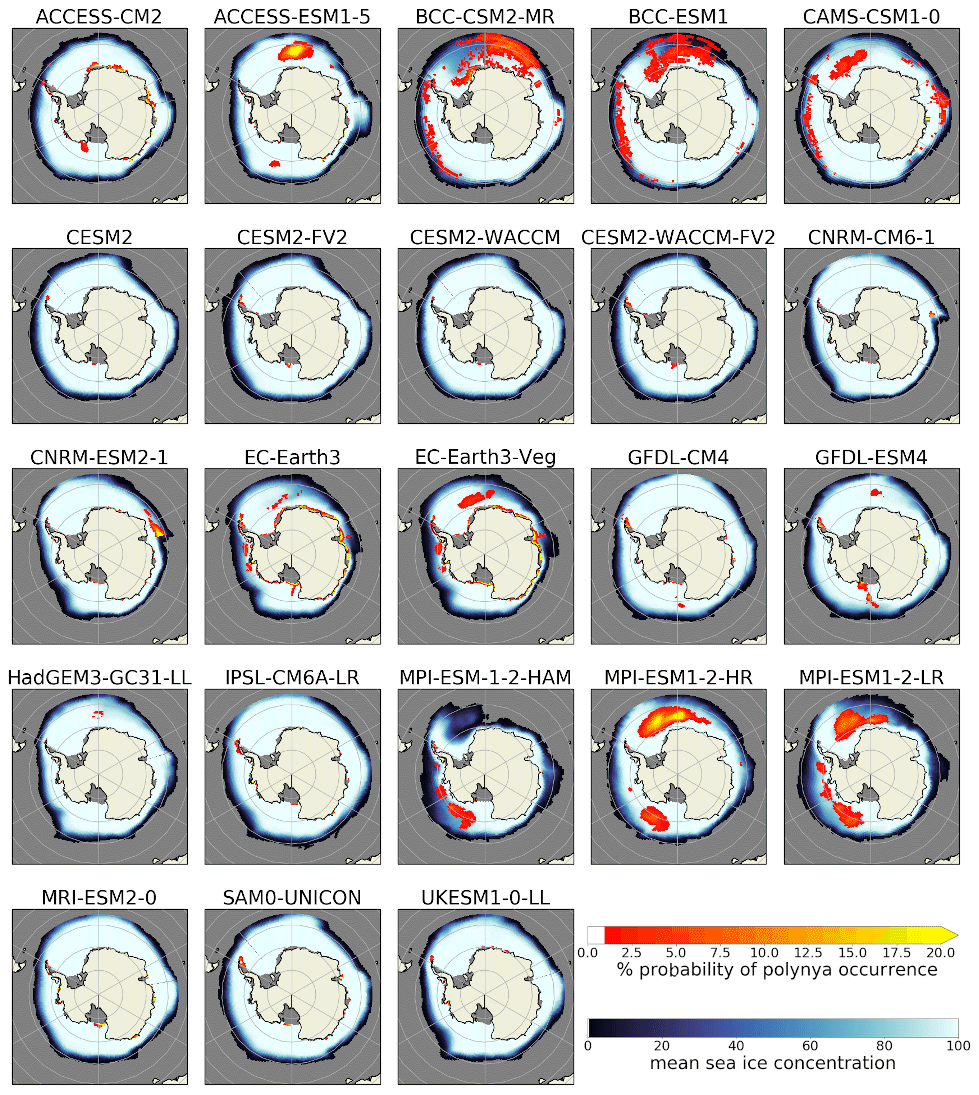
Figure 3Spatial distribution of polynyas in the CMIP6 models, computed from the sea ice thickness output for September. The red-to-yellow colours indicate the number of years where polynyas occurred within the 165 years of the historical model run for each grid cell. The blue colours show the average sea ice concentration (in %).
In agreement with observations, the models show small coastal polynyas during winter that grow in size and in time, merging with other polynyas in spring/summer (November–January; see Figs. 3, 5b or A5). The coastal polynyas are generally located towards the west of geographical features along the continent outlines (Figs. 3, A3 and A4) where the polar easterlies prevail (Barber and Massom, 2007), except for polynyas at the southern end of the western Antarctic Peninsula, which is under the influence of the westerlies and the ACC and thus produces polynyas that are located towards the east of the land. Our analysis includes eight model families (e.g. ACCESS, BCC, CESM2…) that participate in CMIP6 with different model versions (Table 1). Seven of these families show polynyas at very similar locations for all members inside one family (Figs. 3, A3 and A4); the only exception is the ACCESS models. This indicates that the position of polynyas is mostly determined by the model properties and less by coincidence of sporadic polynya occurrence or long-term variability. Comparison of the results from sea ice thickness (Fig. 3) and sea ice concentration (Figs. A4, A3) shows similar locations, but we found on average almost twice the polynya area with the sea ice thickness threshold method (Table 2).
Half of the 27 models show OWPs in the Ross or the Weddell seas. These polynyas are most common close to Maud Rise in the Weddell Sea (Figs. 3, A3 A4). Only 10 models show recurring OWPs in the Weddell Sea: ACCESS-ESM1-5, BCC-(CM2-MR/ESM1), CAMS-CSM1-0, EC-Earth3(-Veg), GFDL-ESM4, HadGEM3-GC31-LL and MPI-ESM1-2-(LR/HR). Of the 23 (28) models that provided sea ice thickness (concentration) output, 6 (8) show, on average, larger OWP than coastal polynya areas, while the remaining 17 (20) models show more coastal polynyas (Fig. 6). Five (fifteen) models overestimate the total polynya area compared to sea ice thickness (concentration) observations. Nine models (ACCESS-CM2, CAMS-CSM1.0, CNRM-CM6, CNRM-CSM2, GFDL-ESM4, all MPIs, UKESM) underestimate the polynya area when derived from the sea ice thickness (12 cm threshold) but at the same time overestimate it when derived from sea ice concentration (30 % threshold). Assuming the observational sea ice concentration product is accurate, this indicates these nine models show too low sea ice concentrations within regions covered by thin sea ice. Overall, the multi-model-spread in the polynya area is large, regardless of whether it is derived from monthly sea ice thickness, monthly concentration or daily concentration ranging from almost no polynyas (SAM0-UNICON) up to 214 930, 64 470 or 80 220 km2 respectively for EC-Earth3-Veg. The multi-model mean is almost twice as high as the observed area (21 880 km2 compared to 10 640 km2 for monthly concentration, 38 560 to 12 050 km2 for daily concentration and 58 680 to 73 060 km2 for monthly sea ice thickness). This is driven primarily by five models; MPI-ESM1-2-HR, ACCESS-CM2, CNRM-ESM2 and the EC-Earth3s all overestimate the polynya area by a factor of 5. Surprisingly, the model ACCESS-CM2 shows only coastal polynyas, while ACCESS-ESM1-5 shows an overabundance of OWPs. These two models share similar versions of the ACCESS-OM2 ocean model component and CICE sea ice model component (Table 1). We further investigate the cause for this difference and its effect on the water stratification in Sect. 5.3.
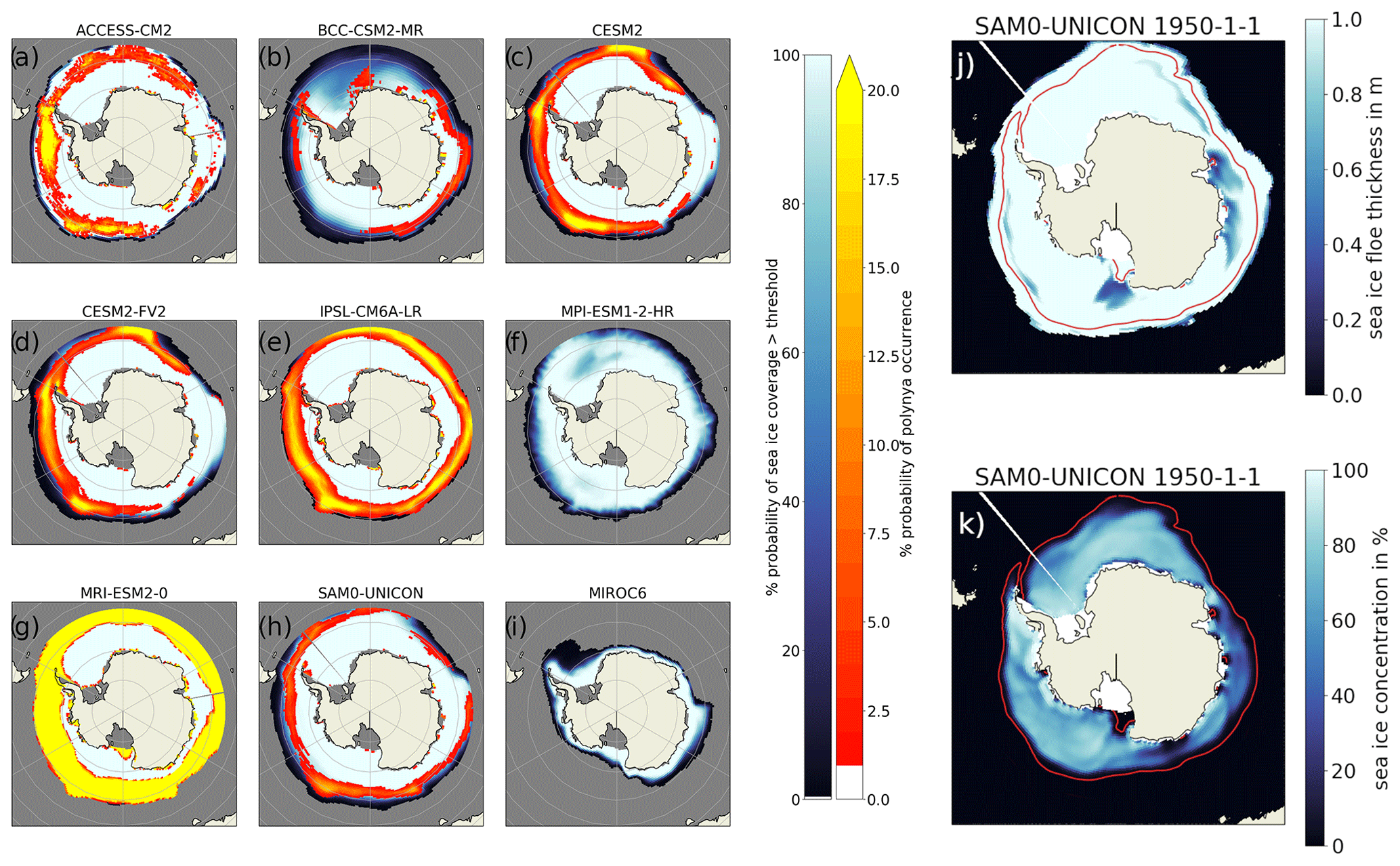
Figure 4(a–i) Unrealistic “polynya areas” computed with a sea ice thickness threshold method from the ice floe thickness output data. (j–k) SAM0-UNICON sea ice floe thickness and sea ice concentration for one time step. The red-to-yellow colours indicate the number of years where polynyas were detected by our algorithm within the 165 years of the historical model run for each grid cell. The blue colours show the average sea ice concentration (in %). The red contour line in panels (j)–(k) marks the 1 % sea ice concentration boundary. Open ocean and ice shelves both appear in grey.
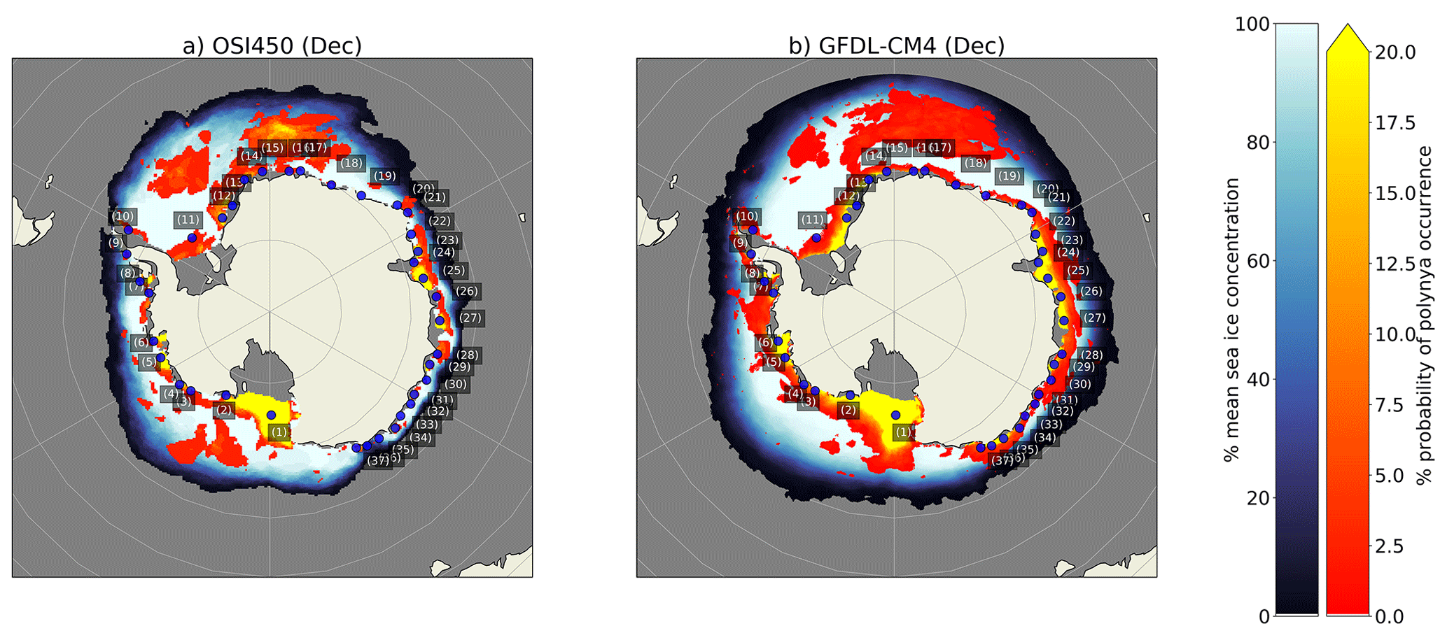
Figure 5Frequency and location of polynya occurrences in December (colours) with the positions of coastal polynyas (blue dots, locations from Arrigo and Van Dijken, 2003) for the common time interval of (a) the observed satellite sea ice (OSI450) and (b) the GFDL-CM4 CMIP6 model with the highest spatial resolution (25×25 km).
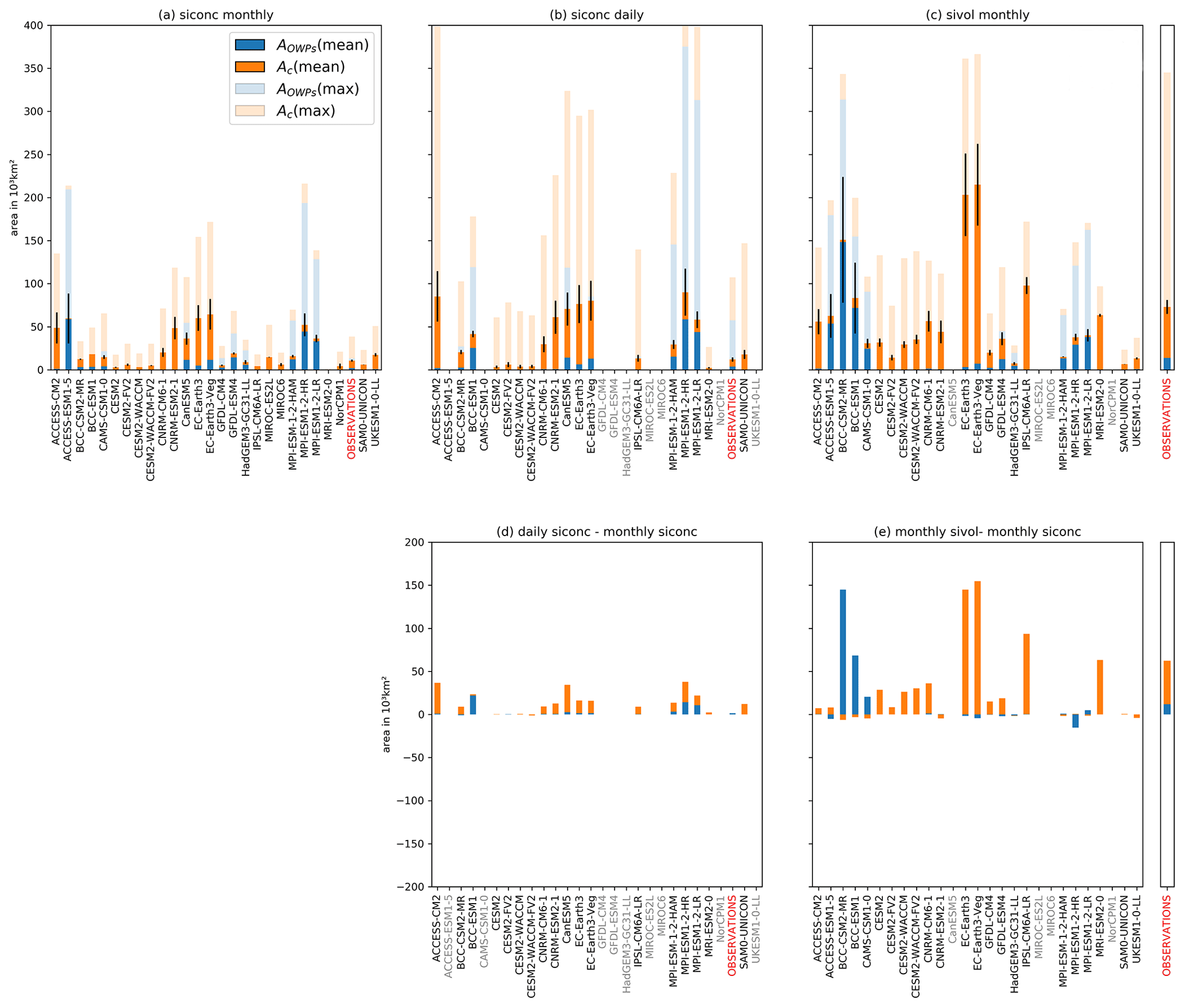
Figure 6Winter polynya area for the CMIP6 models and the observational products (SMOS thin ice and OSI450). The polynyas are computed from (a) monthly sea ice concentration (b) daily sea ice concentration and (c) monthly sea ice thickness. The solid colours mark the yearly mean polynya area, while the transparent colours show the yearly maximum polynya area (Eqs. 1 and 2). The lower panels show the difference in yearly mean polynya area if derived from monthly/daily sea ice concentration (d) and monthly sea ice concentration/thickness (e), for the subset of models that provided both outputs. All data sets were trimmed to the winter period according to Eqs. (1) and (2) respectively, and then the yearly mean from 1979 to and including 2014 for homogenisation in time was formed; the only exception is the observational sea ice thickness, which is not available before 2010 and is presented in a separate panel at its full length until November 2020 at the side of panels (c) and (e). For the mean values in panels (a), (b) and (c), the black bars mark the range in which 50 % of the results are located.
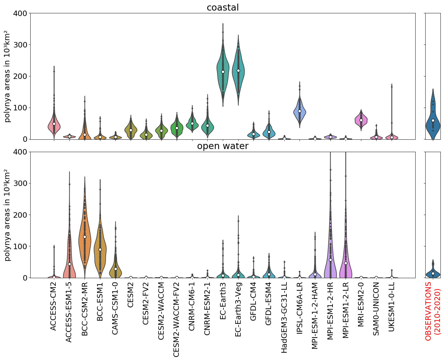
Figure 7Mean total winter polynya area as determined from monthly sea ice thickness for the CMIP6 models and the observational product (SMOS thin ice). For the models, results are shown for the full 165 years of the historical scenario, the observational data set includes the years 2010–2020. Each black dot is an average yearly polynya area for one model. The violin shape indicates the distribution of the values, the most values are in the thickest spot of the violins. The white dot indicates the mean value averaged over all available years.
4.2 Polynya frequency and seasonality
In Sect. 4.1, we discussed the average polynya areas over 35 years. A closer look at individual yearly values from the full historical run reveals that the polynya areas vary from year to year (Fig. 7); for the coastal polynyas the ratio between the year with the largest polynya area to that with the smallest one is at least 2.5 (lowest for MRI-ESM2 and highest for CESM2-FV2, HadGEM3-GC31-LL, MPI-ESM-1-2-HAM and SAM0-UNICON, which have 1 or more years without any coastal polynyas). Models with large coastal polynyas usually have little or no OWPs, while models with large OWPs have few coastal polynyas (Fig. 7). This is most distinct for comparison between the ACCESS models but can also bee seen in comparison of for example MPI to CESM2 models or CAMS-CSM1.0 to MRI-ESM2. The models with a larger fraction of coastal polynyas are ACCESS-CM2, all CESM2s, CNRMs, EC-Earth3s, IPSL-CM6A-LR, MRI-ESM2.0 and UKESM1-0-LL; for the rest the OWPs are dominating. Heuzé (2021) found a negative bottom density bias in the deep ocean for the latter, as they form the Antarctic Bottom Water frequently via deep convection instead of shelf processes. We believe that the deep convection is the reason for the OWPs, because the models that have OWPs mention convective overturning in the Southern Ocean in their model documentation (Table A1), and the water stratification within the polynyas indicates convection (Sect. 4.3). Models without the negative bottom density bias show predominantly coastal polynyas (CESM2s, CanESM5, CNRM-CM6.1, CanESM5, IPSL-CM6A, SAM0-UNICON, UKESM1-0-LL). In contrast to the stratification, numerical choices of parameterisation of open-ocean convective processes were not significant for the presence or absence of deep convection in CMIP5 models (De Lavergne et al., 2014).
The distribution of the OWPs has one fundamental difference to the one for the coastal polynyas. All models except for the BCCs show years without any or with negligible OWP activity (<10 000 km2). The OWP activity we have found in Sect. 4.1 for the EC-Earth3, GFDL and MPI models is mostly caused by some isolated, large-scale OWP events, while the majority of years have little to no OWPs. OWPs in the models are not randomly distributed in time but instead regularly re-open for several consecutive years, as seen in the MPI, ACCESS, BCC, CAMS-CSM1 and EC-Earth models (Figs. 8, A6 and A7). This is interesting since the sea ice in the Weddell Sea melts almost completely every summer. Thus polynya formation must either be facilitated by an external forcing that persists over several years (Campbell et al., 2019, suggest positive SAM fluctuations) or the vertical mixing in OWPs must act as a preconditioning for following years (Martinson et al., 1981). We will discuss this further in Sect. 4.3. While ACCESS-CM2 and BCC-(ESM1/CSM2) show OWPs almost every year, MPI-ESM1.2-(LR/HR), EC-Earth3 and CAMS-CSM1 show episodes of high OWP activity separated by multiple decades of little to no OWPs, as is the case for the real-world Weddell polynya (5 out of 50 years of observation, bottom of Figs. 8, A6, and A7 and Carsey, 1980; Campbell et al., 2019).
For the majority of models, the coastal polynyas appear randomly distributed over the years (Figs. 8, A6 and A7). In agreement with observations, the models show the largest coastal polynyas between November and January (Fig. 9b, c). However, the models underestimate the coastal polynya area in November and December, followed by an equally strong overestimation for January and February (Fig. 9b). The season with the highest OWP activity in the CMIP6 models is between August and November (Fig. 9c, f), while the sea ice observations show a local maximum in polynya occurrence during ice formation in June and an absolute maximum during ice melt in November/December. The seasonality of the OWPs does not agree well between CMIP6 and observations.
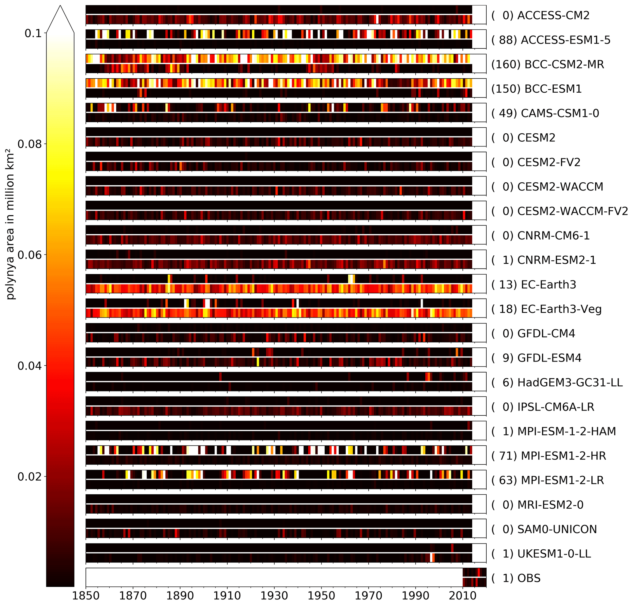
Figure 8Yearly mean polynya area between May and November in the historical CMIP6 model run for the Weddell Sea region computed from the sea ice thickness. Each bar represents one CMIP6 model and is divided horizontally into the coastal polynya area (upper bar) and OWP area (lower bar). The values next to the model name represent the number of years an OWP with an area of more than 10.0×10³ km2 was detected.
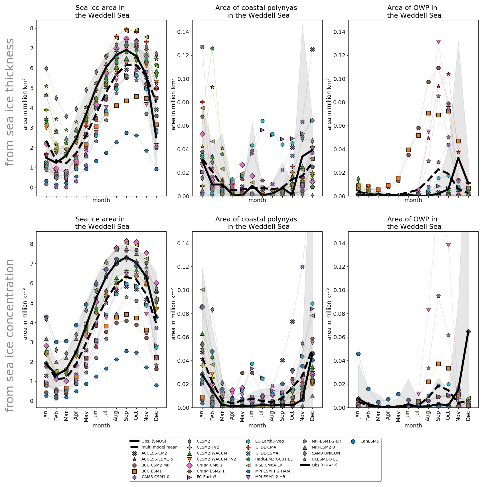
Figure 9Seasonality of (a, d) the sea ice area; (b, e) the coastal polynyas area; and (c, f) the OWP area, for each CMIP6 model (symbols) and the observation products (plain black lines) in the Weddell Sea sector (65∘ W–30∘ E). The areas are derived from CMIP6 sea ice thickness and observational SMOS data (a, b, c) and from CMIP6 sea ice concentrations and observational OSI450 data (d, e, f). Grey shading indicates a 2 standard deviation range from the satellite sea ice data. The data were averaged for the time period 1979–2015.
4.3 Vertical ocean stratification in OWPs
OWPs are strongly influenced by upwelled sensible heat, and they are a source of bottom water production, both in observations (Cheon and Gordon, 2019) and in CMIP models (Heuzé et al., 2013); hence we expect to see a clear difference in the water stratification inside and outside an OWP.
We concentrate on the three models that form most OWPs (MPI-ESM1.2-HR, ACCESS-ESM1.5, BCC-ESM1; see Table 2) and show their vertical profiles in Fig. 10. For comparison, we present the observed hydrographic data of a SOCCOM profiling float (Johnson et al., 2018), which was deployed in January 2015 and surfaced two times in the Maud Rise polynya in winter 2017 (Campbell et al., 2019). To provide regionally and seasonally comparable data sets for the models and the profiling float, we chose to extract vertical profiles during the month of September from within a rectangle around the profiling float trajectory (see Campbell et al., 2019) with the edge coordinates 61–66∘ S, 0–6∘ E in the Weddell Sea. This region includes the northern flank of Maud Rise, where we found OWPs to be most common (Figs. 3, A3, A4).
For the SOCCOM profiling float, we use the information provided in Campbell et al. (2019) to differentiate vertical profiles when the float surfaces within an open-water polynya from those sampled under the sea ice. For the models, we use our algorithm to differentiate and group the grid points by whether they are within an OWP or not. Based on this criterion, we extract and group the monthly vertical salinity and conservative temperature profiles and average spatially over the different vertical profiles to obtain one averaged under-sea-ice profile and one averaged OWP profile (if OWP present in domain) per time step. We plot these profiles then in either blue (under sea ice) or red colour (OWP) in Fig. 10. In comparison to the CMIP6 models, the data of the SOCCOM float are of short length (2015–2017) and limited depth (maximum 2000 m). We hence use additional under-sea-ice profiles from the EN4.2.1 analyses full-depth ocean temperature and salinity data set (Good et al., 2013), limiting it to the same spatial domain as for the CMIP6 models, and show the profiles from 1980–2015 in light grey colour in Fig. 10m–p. We provide the EN4.2.1 data as additional reference of the observed water stratification without major OWP events
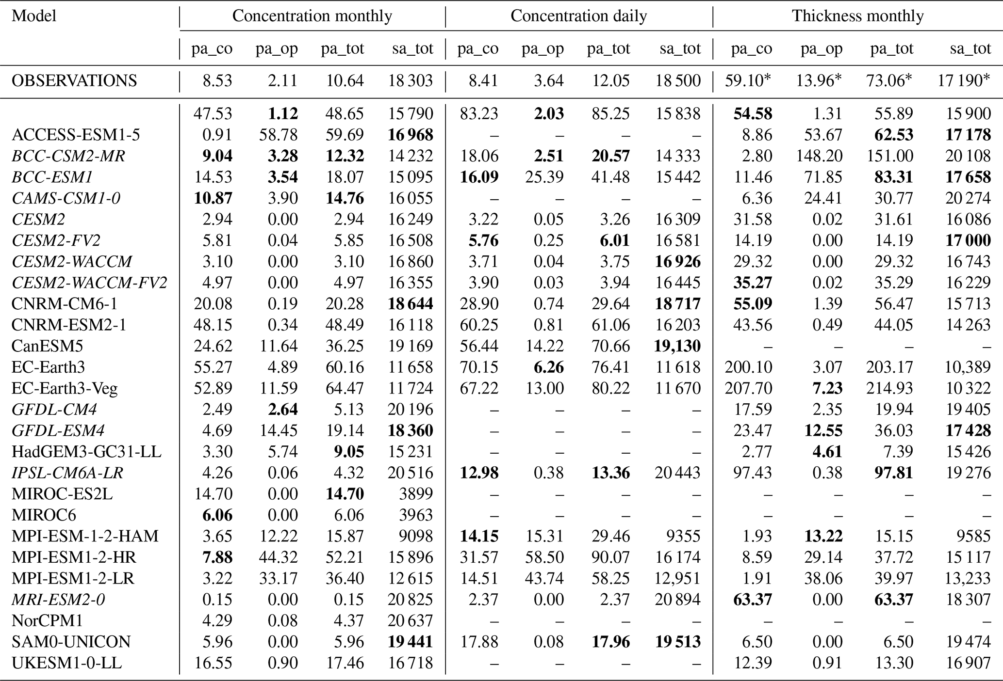
Table 2Mean yearly areas of coastal polynyas (pa_co), OWPs (pa_op), their sum (pa_tot) and the maximum sea ice area (sa_tot) in 103 km2 derived from monthly/daily sea ice concentration and monthly sea ice thickness for September for the complete Southern Ocean, averaged over 1979–2015. Observational sea ice thickness marked with an asterisk (*) is available over a 10-year period only. The four models matching the observations closest are printed in bold, and italic models have a an r value less than 0.8 (Figs. A1 and A2) and thus a relatively weak consistency over the three used sea ice variables.
In the three CMIP6 models, we find major differences in the vertical stratification between the profiles under sea ice and inside OWPs (Fig. 10a–l). In polynyas, deep mixing results in a very weakly stratified water column down to 4000 m, and in particular the salinity difference between mixed layer and Circumpolar Deep Water is reduced by up to 80 % (not shown). This is mainly due to an increased salinity in the upper 1000 m. Close inspection reveals that there is also a reduction in salinity in the Circumpolar Deep Water. Especially for the models MPI-ESM1.2-HR and ACCESS-ESM1.5 we also see a shoaling of the temperature maximum from 824 to 645 and 1560 to 1150 m depth, respectively, and increased temperature from 0.1 to 0.2 ∘C for both models in the upper 500 m of the averaged profile. In the observational profiles (Fig. 10m–p), the temperature maximum can be found at a depth of about 200 m. Compared to the float data, ACCESS-ESM1.5 and BCC-ESM1 underestimate the temperature maximum by 1.5 and 1 ∘C respectively and show it to occur too deep: 1148 ± 132 and 1366 ± 282 m, respectively, under the sea ice and 1560 ± 43 and 1205 ± 389 m, respectively, in OWPs.
In agreement with Cheon and Gordon (2019), we also find that the temperature profiles under the sea ice are more uniform than the profiles within the polynya (Fig. 10). The coldest profiles within polynyas are in fact the least stratified ones. For the model MPI-ESM1.2-HR (Fig. 10a–d), for example, the under-sea-ice temperature varies about 0.5 ∘C from the mean value but varies by more than 1 ∘C inside OWPs. Besides, inside OWPs, some of the profiles have a relatively shallow heat maximum (∼300 m), which is about 0.1 ∘C warmer than the heat maximum under sea ice (Fig. 10b). A possible explanation could be that wind-driven upwelling contributed to a shallowing of the mixed layer depth (MLD) (hence the comparatively shallow heat maximum), leading to increased entrainment of warm CDW into the mixed layer and the opening of an OWP. Upon the opening of the polynya, the water cools rapidly while deep convection occurs, which could explain why the coldest profiles are the least stratified ones. The monthly resolution of the data sets is too low for us to verify these hypotheses.
If the stratification was already weak or the density at the surface is increased by brine rejection of newly formed sea ice, deep convection may commence (weakly stratified cold profiles, Fig. 10). Deep convection reaches different depths in the CMIP models (Fig. 10a–l). MPI-ESM1.2-HR contains some remaining stratification in all profiles, ACCESS-ESM1.5 shows evidence for mixing all the way to the bottom in many profiles and BCC-ESM1 conserves some stratification close to the bottom. In comparison to Argo float measurements, which we found to have undisturbed stable stratification below 500 m even in the polynya profiles, the models show deeper-reaching convection with a portion of the profiles showing no substantial stratification to the bottom (5000 m). However, not all profiles from inside an OWP are homogenised by mixing. About half of the profiles have a shallower and, for the MPI model, warmer temperature maximum compared to the under-ice case. This results in a shallower temperature maximum on average (Fig. 10a, e, i). In comparison to Argo float data, the vertical mixing in the models seems overestimated, which was to be expected as we here selected the subsample of three models with the highest OWP activity. Moreover, the float data contains only two profiles from the very edge of the 2017 Maud Rise polynya event (Campbell et al., 2019), where the vertical mixing may be less prominent than at the polynya's centre. A discussion of the stratification changes from the 1970s Weddell Sea polynya can be found in Cheon and Gordon (2019), where similar mixing as in the CMIP6 models was found.
Re-arranging the profiles into temperature–salinity diagrams (Fig. 10d, h, l, p), the core of the comparatively warm Circumpolar Deep Water (CDW), at approximately 1000 m depth, is easily visible from the temperature maximum. Under sea ice, the water masses on either side of the CDW are clearly separated: the surface layer is cold and fresh, while the deep water is saltier and warmer than the surface. The pycnocline between these layers is at a depth of 100 to 200 m, except for the BCC models, which show very weak stratification, and no clear water mass layers can be identified. Inside the polynyas, the differentiation of the water masses is almost gone (Fig. 10). The models with the highest OWP activity (ACCESS-ESM1.5, BCC and MPI) have low values of the Brunt–Väisälä frequency squared (N2) even under sea ice, where they hardly exceed s−2 (Fig. 10c, g, k, o). The deep mixing transports heat and salt into the surface layer, reducing its density difference compared to deeper layers. This weakened stratification can remain in the water for a significant period of time, preconditioning the region for new polynyas to form in following years (Martinson et al., 1981).
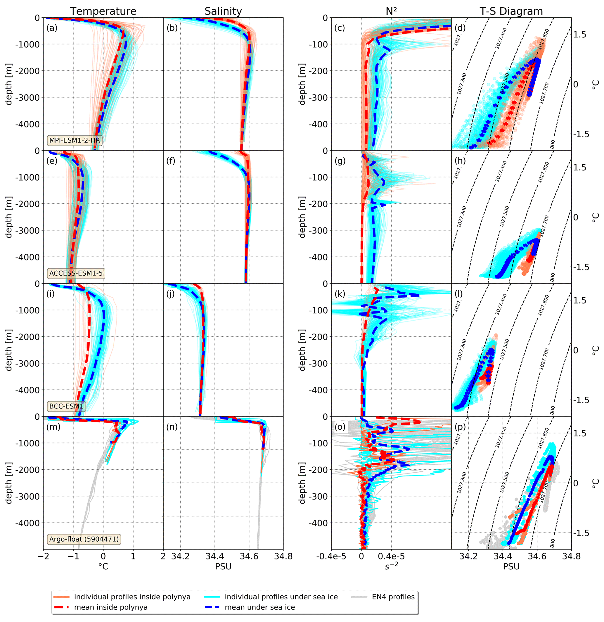
Figure 10Winter profiles occurring within a polynya (red) and under the sea ice (blue, i.e. when no polynya is present) for three representative models (first three rows) and in observations (last row). From left to right: potential temperature, salinity, squared Brunt–Väisälä frequency (N2) and T–S diagram. Note the difference in vertical scale between the first two and the third column. The contour lines in the last column are lines of constant potential density. Two vertical Argo float profiles from within the polynya are available; for comparison we plot 19 under-sea-ice profiles (blue) and monthly September profiles from the EN4.2.1 climatology (grey) in panels (m)–(p).
In the previous sections, we looked at the representation of polynyas in CMIP6 models and their effect on the local water stratification. We found large variations among models, with the majority underestimating OWP area but a few largely overestimating it. The hotspot for OWPs in CMIP6 and observations is the Weddell Sea. Now we want to turn our attention to finding the causes for the difference in polynya activity in the CMIP6 models. We start with a comparison of climate models versus Earth system models and then discuss whether the model's winds and Antarctic Circumpolar Current can explain its OWP representation. Then we examine the possible reasons for the strong overestimation of OWPs in some models and give an outlook about how we expect these biases to change in the near future.
5.1 Polynyas in CM versus ESM versions
The ACCESS, BCC and GFDL families each have two different model configurations for CMIP6: a climate model (CM) version and an Earth system model (ESM) version. In addition to climate physics, ESMs include physical, chemical, and biological processes and interactions and can therefore lead to more realistic climate predictions. Dong et al. (2020) found that the ESM versions have less climate sensitivity compared to the CM versions. We find that the ESM versions show more OWP activity (Fig. 6). The decreased OWP activity we find for CMs in our CMIP6 data set with ongoing global warming is consistent with the results of De Lavergne et al. (2014), in which OWPs in the Weddell Sea eventually stop at the end of the extended CMIP5 climate change runs, as the CM models show a stronger warming response than the ESM versions Dong et al. (2020).
CM models can usually be run at a higher resolution, due to their reduced complexity in comparison to ESMs. GFDL-CM4 has a higher oceanic resolution than GFDL-ESM4 and BCC-CSM2 has a higher atmospheric resolution than BCC-ESM1 (Table 1). A high spatial resolution can improve the representation of katabatic winds and coastlines, which might be why the above-mentioned CMs have a larger fraction of coastal polynyas than their ESM counterparts (Fig. 6). The CM model versions do not only show larger polynya areas (Figs. 6 and 3), but they also show more frequent occurrences of OWPs (Fig. 8). The same trend can be seen between the MPI models, which are alike except for their difference in resolution. The strongest difference in the positions and type of polynyas is found between the ACCESS-CM2 and ACCESS-ESM1.5 models, which show primarily coastal or open-water polynyas respectively (Figs. 3, A3, A4). This difference is further discussed in Sect. 5.3. Our comparison between CM and ESM was only possible on the 3 out of 15 model families that provided both types of model and as such may not apply to the other families. In contrast to our results, De Lavergne et al. (2014) found that deep convection in some CMIP5 models ceases earlier than in ESM models, but likewise their analysis was limited to only three families of models.
5.2 Connections between wind forcing, OWPs and the ACC
Open-water polynya activity is commonly attributed to the SAM, the strength of the Southern Hemisphere winds and the transport of the ACC (e.g. Swart et al., 2018; Cheon et al., 2014; Campbell et al., 2019; Behrens et al., 2016). We combine our polynya characteristics from Sect. 4 with the statistical evaluation of Southern Ocean properties from Beadling et al. (2020) to determine potential across-model relationships between Southern Ocean properties and polynya activity. Since Beadling et al. (2020) present data from 1986–2005, we restrict our analysis to the same period and the 23 models we have in common. The CMIP6 across-model correlation between the total wind stress forcing of the westerlies (Beadling et al., 2020) with OWP activity (Table 2) is 0.49: that is, the models with the strongest Southern Hemisphere westerlies have the highest OWP activity, while the models with the weakest westerlies show no OWP activity (Fig. 11a). We found this correlation to be the same for polynya detection from sea ice concentration and sea ice thickness. The relatively weak correlation coefficients reflects that OWPs cannot be attributed to the wind forcing alone but are sensitive to ocean and atmosphere preconditioning as well as the models' properties as mentioned in Sect. 1.
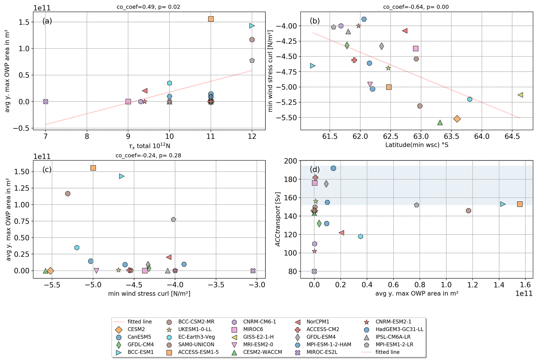
Figure 11Connection of yearly OWP area (as in Eq. 2) with CMIP6 Southern Ocean properties from (Beadling et al., 2020). Total zonally averaged Southern Ocean wind forcing (x) and averaged OWP area (y) (a), linear regression plot of the maximum zonally integrated wind stress curl for each CMIP6 model and the latitude of that maximum (b), wind stress curl minimum (x) and OWP area (y) (c), and OWP area vs. ACC transport (d).
All observed Maud Rise polynyas were preceded by a positive SAM (Campbell et al., 2019). During a positive phase, the westerly wind belt intensifies and contracts towards Antarctica. This process leads to an increased cyclonic wind stress curl and intensifies the Weddell Gyre (Cheon et al., 2014). For the CMIP6 models we found that the maximum strength of the zonally averaged wind stress curl correlates with its latitude (Pearson correlation coefficient of −0.76, computed again using values from Beadling et al., 2020; see Fig. 11b). That means that, unsurprisingly, the CMIP6 models have different average SAM index values. Consequently, we expected an increased OWP activity in the Weddell Sea for the models with the highest wind stress curl maximum. This would consolidate the correlation between SAM and polynya activity. In contrast to Campbell et al. (2019) we find no significant correlation between the wind stress curl maximum and the average OWP area. CMIP6 models temporarily or constantly in a phase with a high SAM index do not show significantly increased OWP activity.
As shown by Hirabara et al. (2012), the ACC transport is positively correlated with OWP activity in observations. Models with an overestimation of OWPs also have too much deep convection (Heuzé, 2021, and Fig. 10), which increases the meridional density gradient and thus enhances the ACC transport (Hirabara et al., 2012; Beadling et al., 2020). The CMIP6 models that feature an ACC in agreement with observational values are ACCESS-CM2, ACCESS-ESM1-5, BCC-ESM1, CanESM5, GFDL-ESM4, IPSL-CM6A-LR, MIROC6, MPI-ESM-1-2-HAM, MPI-ESM1-2-LR and UKESM1-0-LL (Beadling et al., 2020). Nine of these 10 models exhibit open-ocean convection (Heuzé, 2021; see the models marked with an asterisk in Table A1), and in seven we found OWPs (Fig. 11d) in the Southern Ocean. The models ACCESS-CM2, MIROC6 and UKESM1-0-LL did not have large OWPs but excessive deep convection in overly large coastal polynyas (Heuzé, 2021, and Fig. 3) in the open Southern Ocean due to a strong negative sea ice bias (Fig. A3 and Heuzé, 2021; Tatebe et al., 2019) or periodical deep convection in the southern Weddell Sea (Heuzé, 2021). In summary, we find an across-model relationship between the strength of the ACC and OWP activity; models with an overestimation of open-ocean deep convection (which commonly leads to OWPs) are more likely to simulate a realistic ACC transport. Since most models simulate an ACC weaker than the observations (Beadling et al., 2020), an explanation could be that the models suffer in general from insufficient deep water formation, which is weakening the meridional density gradients and vertical stratification, but in turn lead to OWPs in some models that partially compensate for the lack of dense bottom water with spurious deep convection (Heuzé, 2015). Another explanation for this bias could be a general warm bias of the Circumpolar Deep Water (found for CMIP5 models Sallée et al., 2013) that causes OWPs rather than under-sea-ice deep convection (Dufour et al., 2017). We have shown that overabundant OWPs are a common issue in models (Sect. 4.1 and 4.2); that is a problem because it affects the whole water column (Sect. 4.3). We have now found relationships with the models' wider representation of the Southern Ocean, but these relationships have some exceptions. In a case study, we will now investigate the specific case of two seemingly similar models that have extremely different OWP representations, ACCESS-CM2 and ACCESS-ESM1.5.
5.3 Overestimation of OWPs in models and future perspectives
We found that most models overestimate polynya activity in comparison to the observations (Table 2). We believe this to be general knowledge in the community given that within model documentation there are many descriptions of approaches to reduce deep convection and the presence of OWPs in the Southern Ocean (listed and highlighted with an asterisk in Table A1). We first describe approaches to reduce OWPs and conclude with future perspectives. In the previous section, we discussed the correlation of the wind stress curl and ACC transport to polynya activity; we could confirm this in a multi model correlation for the ACC. However, Beadling et al. (2020) found that out of the 34 CMIP6 models they analysed, 29 underestimated the ACC (of which only 12 significantly), 30 showed their wind stress curl not sufficiently south (5 significantly) and 30 underestimated the wind stress curl (WSC) minimum (9 significantly). All these parameters are positively correlated with OWP activity in observations (Campbell et al., 2019). If future model generations are approaching more realistic values for ACC strength, wind stress curl and SAM, we expect that the problem of open-water convection with the formation of large OWP will become evident for even more models.
One of the development foci for the GFDL models was to reduce Southern Ocean polynyas (Held et al., 2019). For the GFDL-CM2 models, the formation of super polynyas in the Southern Ocean was addressed by increasing the near-infrared albedo of glaciers and snow-covered ice caps in order to increase coastal freshwater inflow. This is reported to delay the formation of super polynyas in the model but not to prevent them completely (Held et al., 2019). One reason for this partial success only may be that a realistic representation of the Antarctic Slope Current and related Antarctic Slope Front restricts the lateral spread of fresh water away from the shelf, as Lockwood et al. (2021) found for the GFDL-CM2.6 climate model with a comparatively high horizontal resolution
The CESM2 models feature an overflow parameterisation (Briegleb et al., 2010), which can transport dense bottom water down the shelf and should help with more realistic bottom water formation. This can lead to a more stable stratification, but Heuzé (2015) found that it also caused an overestimation of coastal polynyas in their CMIP5 model version. In our study, we find that the CMIP6 CESM2 models show coastal polynyas, but never OWPs. The observed polynya area is underestimated by at least 30 % by all analysed CESM2 models.
We found that both ACCESS models show more than double the polynya area of the observational data (Figs. 6 and 9). Even though the ACCESS-ESM1.5 and the ACCESS-CM2 models share most model components, the former shows prevalent OWPs, while the latter has mostly coastal polynyas. In the assessment of ACCESS-ESM1.5, Bi et al. (2013) found that OWPs in the Weddell Sea form too often due to deep convection. An iceberg discharge scheme was hence introduced into the model ACCESS-CM2, which freshens and cools the upper ocean (Siobhan O'Farrell, personal communication, June 2020). Fresh water is transported further out into the open ocean instead of entering the ocean directly at the coast. This change effectively suppresses the OWP activity in ACCESS-CM2 (Fig. 3). The freshwater transport of icebergs somewhat suppresses too frequent open-ocean deep convection events (Heuzé, 2021), but ACCESS-CM2 forms too large coastal polynyas instead, much more frequent than ACCESS-ESM1.5. The extent of these coastal polynyas is unrealistically high and the problem of overall too large polynya areas remains. The suppressed OWP activity due to freshwater discharge from icebergs affects the whole water column in the Weddell Sea (Fig. A8). In ACCESS-CM2, the Weddell Deep Water is 0.7 ∘C warmer and the maximum temperature of the CDW is 1.1 ∘C warmer than in ACCESS-ESM1.5.
Here we discussed some examples of modellers' approaches to reduce deep convection and OWPs in the Southern Ocean. In the model documentations (listed in Table A1), we found more examples with the same aim. On the other hand, several models have found a way to prevent these issues. The CESM2 models have an overflow parameterisation (Briegleb et al., 2010) and do not show any OWPs. This parameterisation can provide an effective way for realistic bottom water formation, until higher model resolutions and further model improvements (e.g. better vertical discretisation schemes) allow for actual bottom water formation in coastal polynyas. Also, isopycnal coordinates are beneficial for the representation of down slope flows, the deep water formation in coastal polynyas. This in turn results in more realistic deep water properties (Heuzé et al., 2013). We found that no model with isopycnal coordinates (Table 1) shows an unrealistic amount of OWPs (Table 2 and Fig. 6). The Modular Ocean Model (MOM) introduced isopycnal coordinates in its latest version MOM6. Since several models are based on MOM, e.g. the ACCESS and the BCC models, we expect an improvement in deep water formation, Southern Ocean deep water properties and OWPs when these models successively upgrade to MOM6. Even though isopycnal coordinates were demonstrated to significantly reduce model drift and ocean heat uptake (Adcroft et al., 2019), they also have poor vertical resolution in weakly stratified regions such as the Weddell Sea and cannot avoid spurious deep convection in all cases. Only in combination with adequate implementation of shelf processes and dense water overflows, optimal results could be obtained (Adcroft et al., 2019).
In this paper, we evaluated the representation of Southern Ocean open-water and coastal polynyas in CMIP6 climate models and their effects on the modelled Weddell Sea. We found the following:
-
all 27 analysed models have coastal polynyas around the Antarctic continent, while OWPs are present in only half of the models;
-
CMIP6 models show OWPs most commonly either in the Weddell or the Ross seas;
-
the position of polynya formation is very similar for models in one family and likely determined by the model properties;
-
in comparison to observations, nine models underestimate polynya areas based on thickness threshold but overestimate them if based on the concentration threshold method;
-
coastal polynya areas in CMIP6 have a large annual variability of at least a factor of 2.5;
-
with total polynya areas from 6.5×10³ up to 215×103 km2, CMIP6 models show a large model spread.
Based on the results from the sea ice thickness, the models ACCESS-ESM1.5, BCC-ESM1 and MRI-ESM2.0 show the best agreement in total polynya area with less than 15 % deviation from observations, but ACCESS-ESM1.5 and BCC-ESM1 show a strong bias towards OWPs and MRI-ESM2.0 has only coastal polynyas. The inconsistent representation of polynyas can be problematic, since polynyas account for large amounts of sea ice and deep water production. We found larger polynyas with the sea ice thickness threshold method in 19 of 23 models and the observational data, and 4 models showed larger total polynya areas with the sea ice concentration threshold method. Using monthly sea ice concentration data instead of daily data leads to an underestimation of the polynya area in all models and the observations.
We have shown how OWPs significantly reduce the local stratification. We found indications of deep convection, which eventually change the long-term water properties in the Weddell Sea, notably removing the stratification and hence making future polynyas more likely. In Sect. 5.3 we discussed how the problem of spurious open-ocean deep convection in many CMIP6 models may be related to the OWPs biases. Half of the CMIP6 models show an over-representation of OWPs (Table 2), which is a known problem in the field (e.g. Held et al., 2019; Gutjahr et al., 2019; Sellar et al., 2019), likely caused by unrealistic deep convection events in the Southern Ocean (see Table A1, for references). We have described some of the models' strategies to prevent open-ocean polynyas and their caveats. CMIP6 models with realistic representation of the ACC transport and Southern Ocean wind fields commonly show unrealistically increased OWP formation in the Weddell Sea (Sect. 5.2). At the same time, future increases of the horizontal model resolution, improved vertical discretisation schemes, overflow parameterisations and freshwater influxes will likely help to achieve more realistic representations of polynyas in the Southern Ocean and in sea-ice-covered polar regions in general.
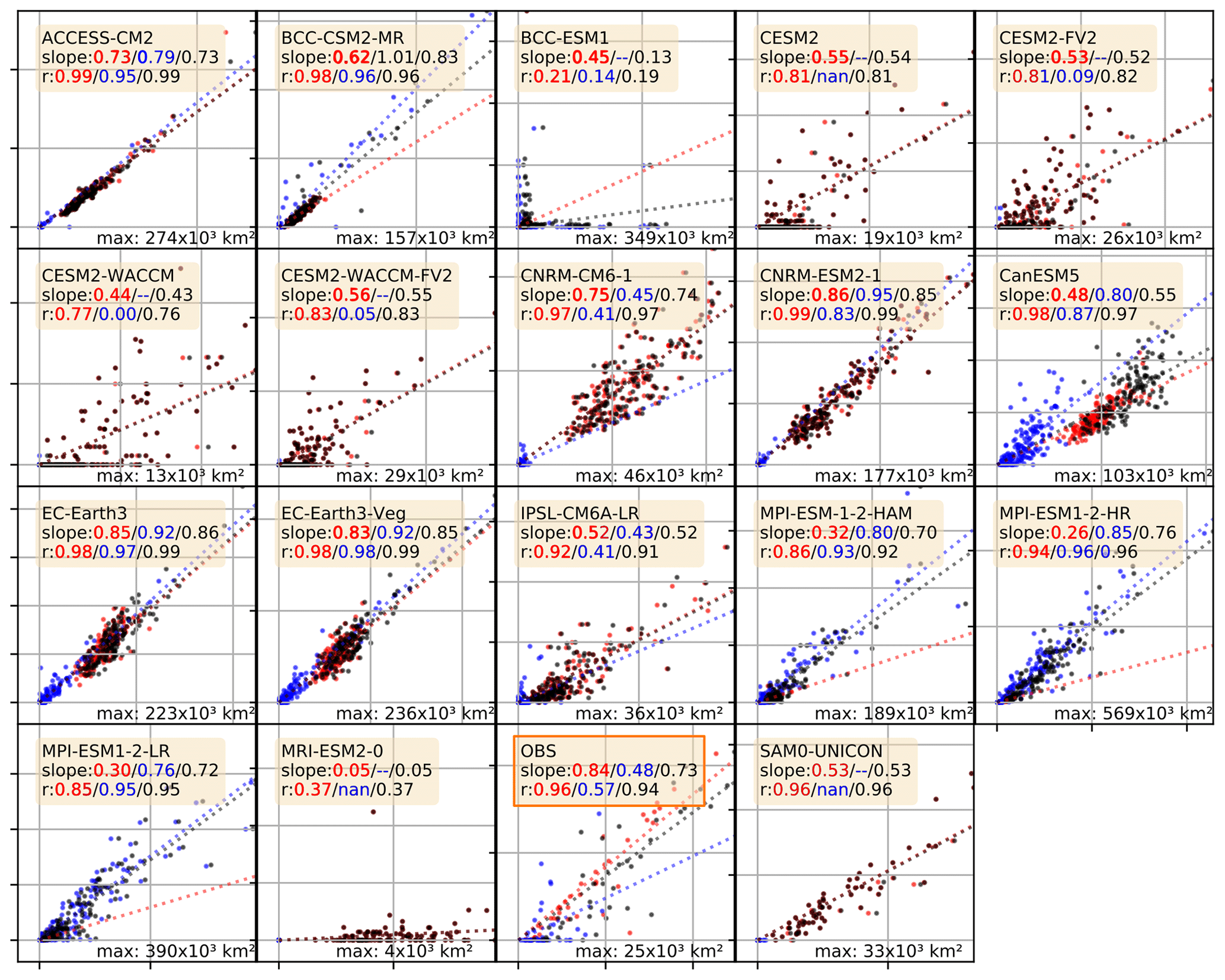
Figure A1Correlation plots for the polynya areas computed from daily (x) vs. monthly (y) sea ice concentrations as presented in Table 2. Each dot represents the averaged polynya area of one year; red are the coastal polynyas, blue the OWPs and black the sum of both. Where applicable (e.g. polynyas present, p value <0.05) the legend includes the slopes of the correlation in the order coastal/open-water/combined polynyas. Because the area of polynyas varies by more than 1 order of magnitude, we normalised the axes of each plot by the highest numerical value for each model and give its value in the lower right corner of each plot.
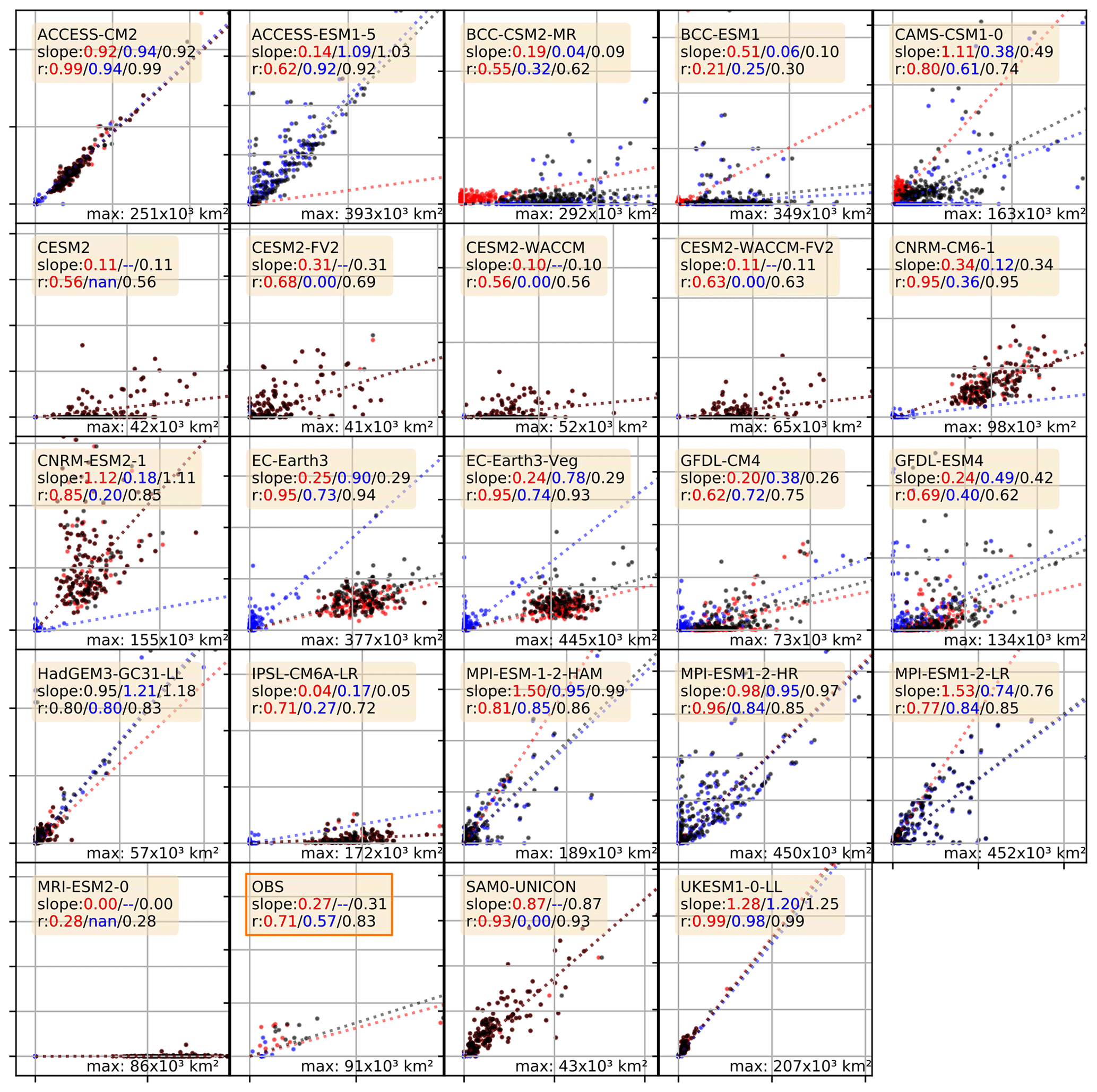
Figure A2Correlation plots for the polynya areas computed from monthly sea ice thickness (x) vs. monthly sea ice concentration (y) as presented in Table 2. Each dot represents the averaged polynya area of 1 year; red are the coastal polynyas, blue the OWPs and black the sum of both. Where applicable (e.g. polynyas present, p value <0.05) the legend includes the slopes of the correlation in the order coastal/open-water/combined polynyas. Because the area of polynyas varies by more than 1 order of magnitude, we normalised the axes of each plot by the highest numerical value for each model and give its value in the lower right corner of each plot.
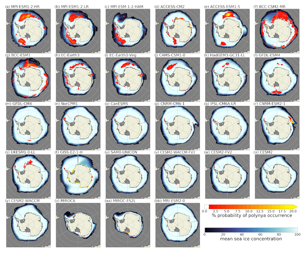
Figure A3Spatial distribution of polynyas in the CMIP6 models, computed from the monthly sea ice concentration output for September. The red-to-yellow colours indicate the number of years where polynyas occurred within the 165 years of the historical model run for each grid cell. The blue colours show the average sea ice concentration (in %).
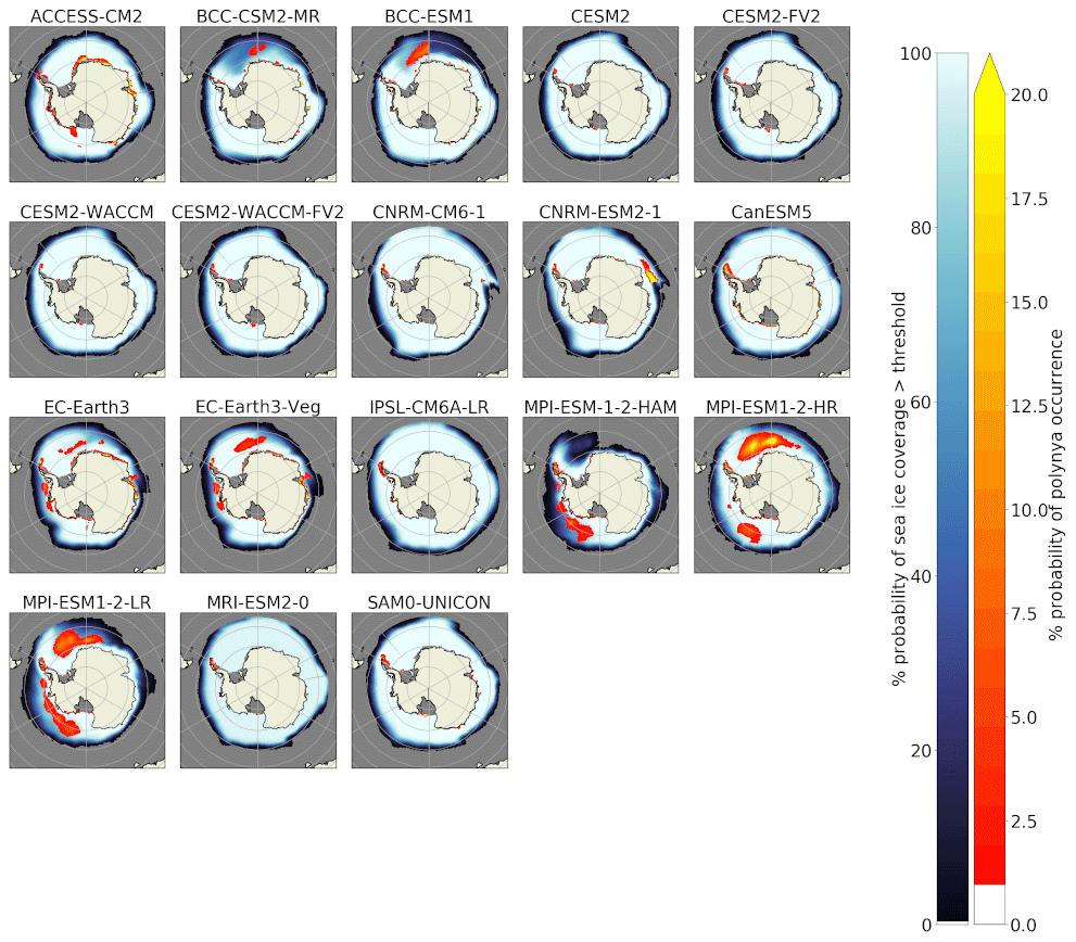
Figure A4Spatial distribution of polynyas in the CMIP6 models, computed from the daily sea ice concentration output for September. The red-to-yellow colours indicate the number of years where polynyas occurred within the 165 years of the historical model run for each grid cell. The blue colours show the average sea ice concentration (in %).
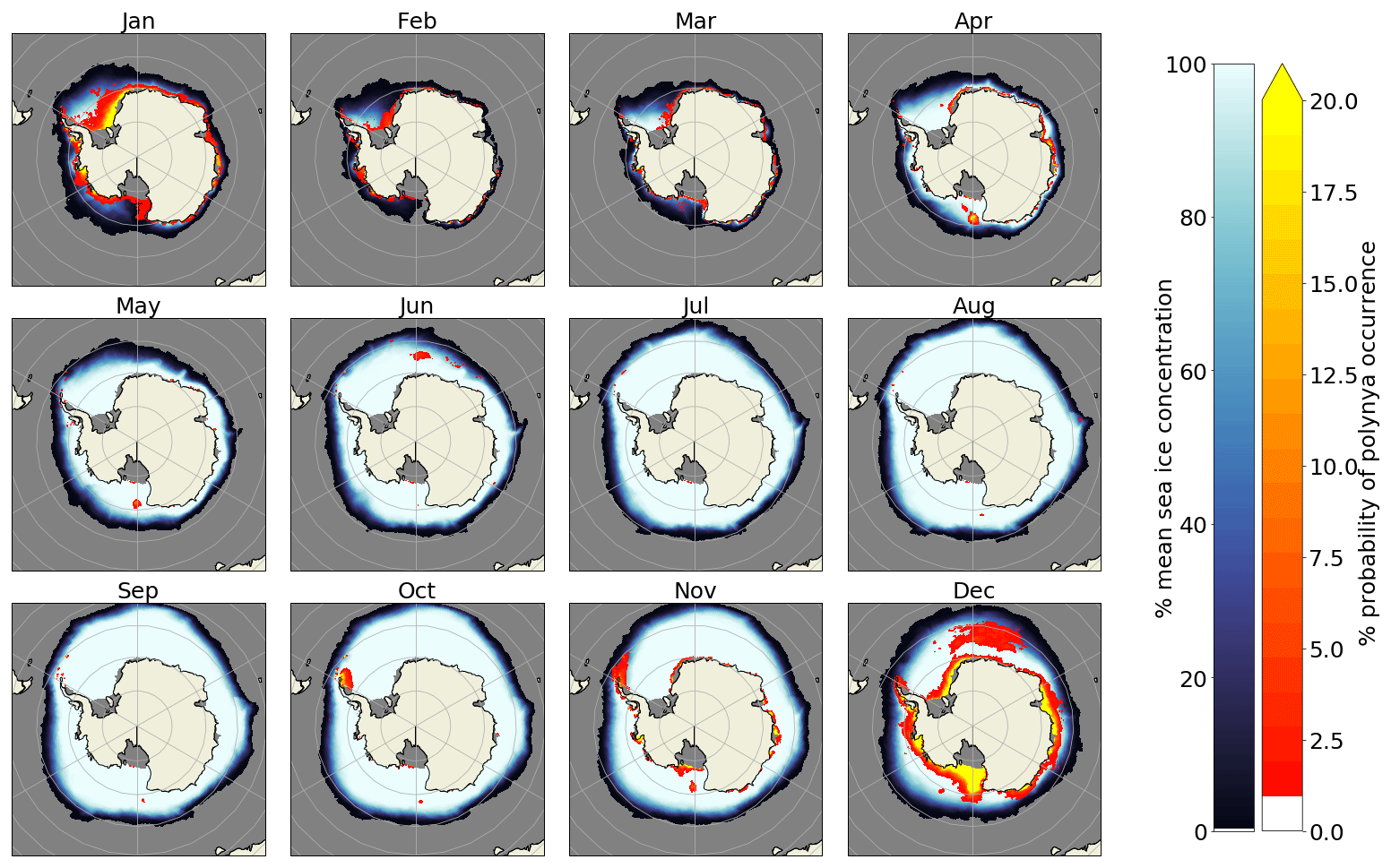
Figure A5The seasonal cycle of sea ice concentration (blue colours) and polynya probability (red–yellow) for the GFDL-CM4 model.

Figure A6Yearly mean polynya area between May and November in the historical CMIP6 model run for the Weddell Sea region, computed from monthly sea ice concentrations. Each bar represents one CMIP6 model and is divided horizontally into coastal polynya area (upper bar) and OWP area (lower bar). The values next to the model name represent the number of years an open-water polynya with an area of more than 10.0×10³ km2 was detected.
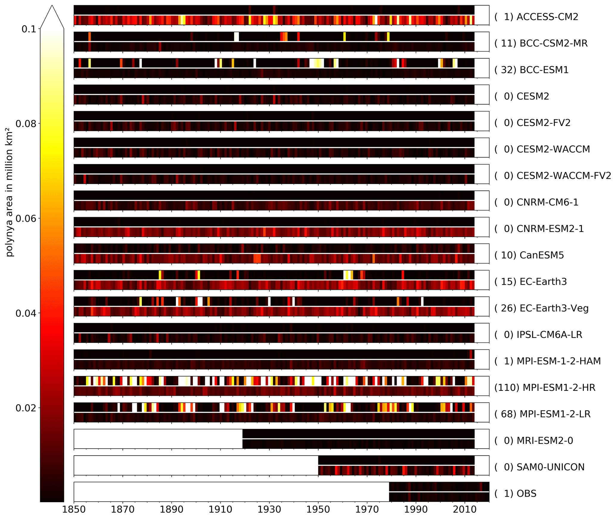
Figure A7Yearly mean polynya area between May and November in the historical CMIP6 model run for the Weddell Sea region, computed from daily sea ice concentrations. Each bar represents one CMIP6 model and is divided horizontally into coastal polynya area (upper bar) and OWP area (lower bar). The values next to the model name represent the number of years an open-water polynya with an area of more than 10.0×10³ km2 was detected.
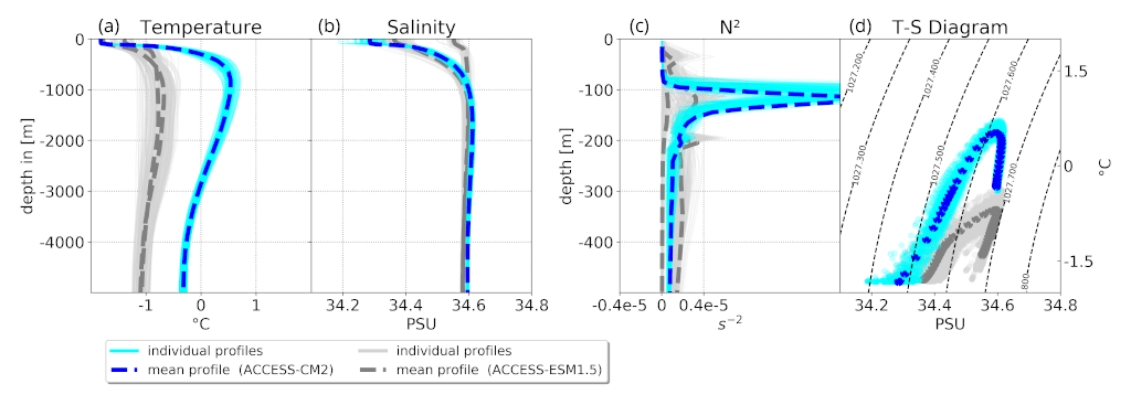
Figure A8Comparison of the winter profiles of the CMIP6 models ACCESS-ESM1.5 (blue) and ACCESS-CM2 (grey). From left to right: temperature, salinity, Brunt–Väisälä frequency N2 and T–S diagram.
Table A1The 28 CMIP6 models used in this study (full name and references with model description). The references marked with an asterisk (*) contain information about deep convection in the Southern Ocean. N/A indicates that no paper has been published yet for the CMIP6 configuration.
The code to reproduce the analysis is freely available at https://github.com/MartinMohrmann/Southern-Ocean-polynyas-in-CMIP6-models (last access: December 2020) and https://doi.org/10.5281/zenodo.5187947 (Mohrmann et al., 2021).
CMIP6 data are freely available via any portal of the Earth System Grid Federation; a list over the different portals to download the data can be found at https://esgf-node.llnl.gov/projects/cmip6/ (CMIP, 2020).
The observational sea ice concentration products OSI450 and OSI-430-b (Lavergne et al., 2019) are provided by the Norwegian and Danish meteorological institutes online: https://doi.org/10.15770/EUM_SAF_OSI_0008 (OSI SAF, 2017). The observational product for thickness of thin sea ice (SIT) is available via ftp at https://seaice.uni-bremen.de/data/smos (Huntemann and Heygster, 2020). The float data are freely available via the Southern Ocean Carbon and Climate Observations and Modeling (SOCCOM) Float Data Archive (https://doi.org/10.6075/J02J6968, Johnson et al., 2018).
MM, CH and SS designed the study. MM conducted the analyses under the supervision of CH and SS. MM and CH wrote the paper.
The authors declare that they have no conflict of interest.
Publisher's note: Copernicus Publications remains neutral with regard to jurisdictional claims in published maps and institutional affiliations.
We are thankful for the comments of David Schroeder on a previous version of this paper. We also thank the anonymous reviewer, Carolina Dufour and Rebecca Beadling for their comments, which greatly helped us improve the quality of our writing and frame the presented research in a wider scientific context.
We acknowledge the World Climate Research Programme, which made this paper possible by coordinating and promoting CMIP6. We thank the climate modelling groups listed in Tables 1 and A1 for producing, unifying and providing their output; the Earth System Grid Federation (ESGF) for archiving the data and providing access; and the multiple funding agencies who support CMIP6 and ESGF. Data were collected and made freely available by the Southern Ocean Carbon and Climate Observations and Modeling (SOCCOM) Project funded by the National Science Foundation, Division of Polar Programs (NSF PLR-1425989), supplemented by NASA, and by the international Argo programme and the NOAA programmes that contribute to it. The Argo programme is part of the Global Ocean Observing System (https://doi.org/10.17882/42182, http://argo.jcommops.org, last access: October 2020).
We acknowledge the support from the Oceanography Marks Foundation (Knut J:son Mark) at GU for financial support of PhD studies. Céline Heuzé is funded by the Swedish National Space Agency (164/18) and the Swedish Research Council (VR 2018-03859). Sebastiaan Swart acknowledges support from the following grants: Wallenberg Academy Fellowship (WAF 2015.0186), Swedish Research Council (VR 2019-04400), STINT-NRF Mobility Grant and NRF-SANAP (SNA170522231782).
This paper was edited by Nicolas Jourdain and reviewed by Carolina Dufour and one anonymous referee.
Adcroft, A., Anderson, W., Balaji, V., Blanton, C., Bushuk, M., Dufour, C. O., Dunne, J. P., Griffies, S. M., Hallberg, R., Harrison, M. J., Held, I. M., Jansen, M. F., John, J. G., Krasting, J. P., Langenhorst, A. R., Legg, S., Liang, Z., McHugh, C., Radhakrishnan, A., Reichl, B. G., Rosati, T., Samuels, B. L., Shao, A., Stouffer, R., Winton, M., Wittenberg, A. T., Xiang, B., Zadeh, N., and Zhang, R.: The GFDL global ocean and sea ice model OM4.0: Model description and simulation features, J. Adv. Model. Earth Sy., 11, 3167–3211, 2019. a, b
Aguiar, W., Mata, M. M., and Kerr, R.: On deep convection events and Antarctic Bottom Water formation in ocean reanalysis products, Ocean Sci., 13, 851–872, https://doi.org/10.5194/os-13-851-2017, 2017. a
Andreas, E. L. and Ackley, S. F.: On the differences in ablation seasons of Arctic and Antarctic sea ice, J. Atmos. Sci., 39, 440–447, 1982. a
Arbetter, T. E., Lynch, A. H., and Bailey, D. A.: Relationship between synoptic forcing and polynya formation in the Cosmonaut Sea: 1. Polynya climatology, J. Geophys. Res.-Oceans, 109, C04022, https://doi.org/10.1029/2003JC001837, 2004. a
Arrigo, K. R. and Van Dijken, G. L.: Phytoplankton dynamics within 37 Antarctic coastal polynya systems, J. Geophys. Res.-Oceans, 108, 3271, https://doi.org/10.1029/2002JC001739, 2003. a
Barber, D. G. and Massom, R. A.: The role of sea ice in Arctic and Antarctic polynyas, Elsev. Oceanogr. Series, 74, 1–54, 2007. a
Beadling, R., Russell, J., Stouffer, R., Mazloff, M., Talley, L., Goodman, P., Sallée, J., Hewitt, H., Hyder, P., and Pandde, A.: Representation of Southern Ocean Properties across Coupled Model Intercomparison Project Generations: CMIP3 to CMIP6, J. Climate, 33, 6555–6581, 2020. a, b, c, d, e, f, g, h, i, j, k, l
Behrens, E., Rickard, G., Morgenstern, O., Martin, T., Osprey, A., and Joshi, M.: Southern Ocean deep convection in global climate models: A driver for variability of subpolar gyres and Drake Passage transport on decadal timescales, J. Geophys. Res.-Oceans, 121, 3905–3925, 2016. a, b
Bi, D., Dix, M., Marsland, S. J., O’Farrell, S., Rashid, H., Uotila, P., Hirst, A. C., Kowalczyk, E., Golebiewski, M., Sullivan, A., Yan, Y., Hannah, N., Franklin, C., Sun, Z., Vohralik, P., Watterson, I., Fiedler, R., Collier, M., and Puri, K.: The ACCESS coupled model: description, control climate and evaluation, Aust. Meteorol. Oceanogr. J., 63, 41–64, 2013. a, b, c
oucher, O., Servonnat, J., Albright, A. L., Aumont, O., Balkanski, Y., Bastrikov, V., Bekki, S., Bonnet, R., Bony, S., Bopp, L., Braconnot, P., Brockmann, P., Cadule, P., Caubel, A., Cheruy, F., Codron, F., Cozic, A., Cugnet, D., D'Andrea, F., Davini, P., de Lavergne, C., Denvil, S., Deshayes, J., Devilliers, M., Ducharne, A., Dufresne, J.-L., Dupont, E., Éthé, C., Fairhead, L., Falletti, L., Flavoni, S., Foujols, M.-A., Gardoll, S., Gastineau, G., Ghattas, J., Grandpeix, J.-Y., Guenet, B., Guez, Lionel, E., Guilyardi, E., Guimberteau, M., Hauglustaine, D., Hourdin, F., Idelkadi, A., Joussaume, S., Kageyama, M., Khodri, M., Krinner, G., Lebas, N., Levavasseur, G., Lévy, C., Li, L., Lott, F., Lurton, T., Luyssaert, S., Madec, G., Madeleine, J.-B., Maignan, F., Marchand, M., Marti, O., Mellul, L., Meurdesoif, Y., Mignot, J., Musat, I., Ottlé, C., Peylin, P., Planton, Y., Polcher, J., Rio, C., Rochetin, N., Rousset, C., Sepulchre, P., Sima, A., Swingedouw, D., Thiéblemont, R., Traore, A. K., Vancoppenolle, M., Vial, J., Vialard, J., Viovy, N., and Vuichard, N.: Presentation and evaluation of the IPSL-CM6A-LR climate model, J. Adv. Model. Earth Sy., 12, e2019MS002010, https://doi.org/10.1029/2019MS002010, 2020. a
Briegleb, B., Danabasoglu, G., and Large, W.: An overflow parameterization for the ocean component of the Community Climate System Model, NCAR Tech, Tech. rep., Note NCAR/TN-481+ STR, Draft, 72 pp., 2010. a, b
Campbell, E. C., Wilson, E. A., Moore, G. K., Riser, S. C., Brayton, C. E., Mazloff, M. R., and Talley, L. D.: Antarctic offshore polynyas linked to Southern Hemisphere climate anomalies, Nature, 570, 319–325, 2019. a, b, c, d, e, f, g, h, i, j, k, l
Carsey, F.: Microwave observation of the Weddell Polynya, Mon. Weather Rev., 108, 2032–2044, 1980. a, b
Cheon, W. G. and Gordon, A. L.: Open-ocean polynyas and deep convection in the Southern Ocean, Sci. Rep., 9, 1–9, 2019. a, b, c, d, e, f, g
Cheon, W. G., Park, Y.-G., Toggweiler, J., and Lee, S.-K.: The relationship of Weddell Polynya and open-ocean deep convection to the Southern Hemisphere westerlies, J. Phys. Oceanogr., 44, 694–713, 2014. a, b, c
CMIP: Coupled Model Intercomparison Project Phase 6 (CMIP6) data, Working Group on Coupled Modeling of the World Climate Research Programme, Earth System Grid Federation [data set], available at: https://esgf-data.dkrz.de/projects/cmip6-dkrz/, last access: December 2020. a
Counillon, F., Keenlyside, N., Bethke, I., Wang, Y., Billeau, S., Shen, M. L., and Bentsen, M.: Flow-dependent assimilation of sea surface temperature in isopycnal coordinates with the Norwegian Climate Prediction Model, Tellus A, 68, 32437, https://doi.org/10.3402/tellusa.v68.32437 2016. a, b
Danabasoglu, G., Lamarque, J.-F., Bacmeister, J., Bailey, D. A., DuVivier, A. K., Edwards, J., Emmons, L. K., Fasullo, J., Garcia, R., Gettelman, A., Hannay, C., Holland, M. M., Large, W. G., Lauritzen, P. H., Lawrence, D. M., Lenaerts, J. T. M., Lindsay, K., Lipscomb, W. H., Mills, M. J., Neale, R., Oleson, K. W., Otto-Bliesner, B., Phillips, A. S., Sacks, W., Tilmes, S., van Kampenhout, L., Vertenstein, M., Bertini, A., Dennis, J., Deser, C., Fischer, C., Fox-Kemper, B., Kay, J. E., Kinnison, D., Kushner, P. J., Larson, V. E., Long, M. C., Mickelson, S., Moore, J. K., Nienhouse, E., Polvani, L., Rasch, P. J., and Strand, W. G.: The Community Earth System Model version 2 (CESM2), J. Adv. Model. Earth Sy., 12, e2019MS001916, https://doi.org/10.1029/2019MS001916, 2020. a, b, c, d
Dee, D. P., Uppala, S. M., Simmons, A. J., Berrisford, P., Poli, P., Kobayashi, S., Andrae, U., Balmaseda, M. A., Balsamo, G., Bauer, P., Bechtold, P., Beljaars, A. C. M., van de Berg, L., Bidlot, J., Bormann, N., Delsol, C., Dragani, R., Fuentes, M., Geer, A. J., Haimberger, L., Healy, S. B., Hersbach, H., Hólm, E. V., Isaksen, L., Kållberg, P., Köhler, M., Matricardi, M., McNally, A. P., Monge-Sanz, B. M., Morcrette, J.-J., Park, B.-K., Peubey, C., de Rosnay, P., Tavolato, C., Thépaut, J.-N., and Vitart, F.: The ERA-Interim reanalysis: Configuration and performance of the data assimilation system, Q. J. Roy. Meteor. Soc., 137, 553–597, 2011. a
De Lavergne, C., Palter, J. B., Galbraith, E. D., Bernardello, R., and Marinov, I.: Cessation of deep convection in the open Southern Ocean under anthropogenic climate change, Nat. Clim. Change, 4, 278–282, 2014. a, b, c, d
Dong, Y., Armour, K. C., Zelinka, M. D., Proistosescu, C., Battisti, D. S., Zhou, C., and Andrews, T.: Intermodel Spread in the Pattern Effect and Its Contribution to Climate Sensitivity in CMIP5 and CMIP6 Models, J. Climate, 33, 7755–7775, https://doi.org/10.1175/JCLI-D-19-1011.1, 2020. a, b
Dufour, C. O., Morrison, A. K., Griffies, S. M., Frenger, I., Zanowski, H., and Winton, M.: Preconditioning of the Weddell Sea polynya by the ocean mesoscale and dense water overflows, J. Climate, 30, 7719–7737, 2017. a, b, c, d
Dunne, J. P., Horowitz, L. W., Adcroft, A. J., Ginoux, P., Held, I. M., John, J. G., Krasting, J. P., Malyshev, S., Naik, V., Paulot, F., Shevliakova, E., Stock, C. A., Zadeh, N., Balaji, V., Blanton, C., Dunne, K. A., Dupuis, C., Durachta, J., Dussin, R., Gauthier, P. P. G., Griffies, S. M., Guo, H., Hallberg, R. W., Harrison, M., He, J., Hurlin, W., McHugh, C., Menzel, R., Milly, P. C. D., Nikonov, S., Paynter, D. J., Ploshay, J., Radhakrishnan, A., Rand, K., Reichl, B. G., Robinson, T., Schwarzkopf, D. M., Sentman, L. T., Underwood, S., Vahlenkamp, H., Winton, M., Wittenberg, A. T., Wyman, B., Zeng, Y., and Zhao, M.: The GFDL Earth System Model version 4.1 (GFDL-ESM4.1): Model description and simulation characteristics (under review), J. Adv. Model. Earth Sy., 11, 3167–3211, 2019. a
Eyring, V., Bony, S., Meehl, G. A., Senior, C. A., Stevens, B., Stouffer, R. J., and Taylor, K. E.: Overview of the Coupled Model Intercomparison Project Phase 6 (CMIP6) experimental design and organization, Geosci. Model Dev., 9, 1937–1958, https://doi.org/10.5194/gmd-9-1937-2016, 2016. a, b
Francis, D., Eayrs, C., Cuesta, J., and Holland, D.: Polar cyclones at the origin of the reoccurrence of the Maud Rise Polynya in austral winter 2017, J. Geophys. Res.-Atmos., 124, 5251–5267, 2019. a
Good, S., Martin, M., and Rayner, N.: EN4: quality controlled ocean temperature and salinity profiles and monthly objective analyses with uncertainty estimates, J. Geophys. Res.-Oceans, 118, 6704–6716, 2013. a
Gordon, A. L., Visbeck, M., and Comiso, J. C.: A possible link between the Weddell Polynya and the Southern Annular Mode, J. Climate, 20, 2558–2571, 2007. a, b
Gutjahr, O., Putrasahan, D., Lohmann, K., Jungclaus, J. H., von Storch, J.-S., Brüggemann, N., Haak, H., and Stössel, A.: Max Planck Institute Earth System Model (MPI-ESM1.2) for the High-Resolution Model Intercomparison Project (HighResMIP), Geosci. Model Dev., 12, 3241–3281, https://doi.org/10.5194/gmd-12-3241-2019, 2019. a, b, c
Hajima, T., Watanabe, M., Yamamoto, A., Tatebe, H., Noguchi, M. A., Abe, M., Ohgaito, R., Ito, A., Yamazaki, D., Okajima, H., Ito, A., Takata, K., Ogochi, K., Watanabe, S., and Kawamiya, M.: Development of the MIROC-ES2L Earth system model and the evaluation of biogeochemical processes and feedbacks, Geosci. Model Dev., 13, 2197–2244, https://doi.org/10.5194/gmd-13-2197-2020, 2020. a
Hasumi, H.: CCSR ocean component model (COCO), Atmosphere and Ocean Research Institute,The University of Tokyo, 5-1-5 Kashiwanoha, Kashiwa, Chiba 277-8568, Japan, 2015. a
Held, I. M., Guo, H., Adcroft, A., Dunne, J. P., Horowitz, L. W., Krasting, J., Shevliakova, E., Winton, M., Zhao, M., Bushuk, M., Wittenberg, A. T., Wyman, B., Xiang, B., Zhang, R., Anderson, W., Balaji, V., Donner, L., Dunne, K., Durachta, J., Gauthier, P. P. G., Ginoux, P., Golaz, J.-C., Griffies, S. M., Hallberg, R., Harris, L., Harrison, M., Hurlin, W., John, J., Lin, P., Lin, S.-J., Malyshev, S., Menzel, R., Milly, P. C. D., Ming, Y., Naik, V., Paynter, D., Paulot, F., Rammaswamy, V., Reichl, B., Robinson, T., Rosati, A., Seman, C., Silvers, L. G., Underwood, S., and Zadeh, N.: Structure and performance of GFDL's CM4.0 climate model, J. Adv. Model. Earth Sy., 11, 3691–3727, 2019. a, b, c, d, e
Heuzé, C.: Antarctic Bottom Water in CMIP5 models: characteristics, formation, evolution, PhD thesis, University of East Anglia, 2015. a, b, c, d
Heuzé, C.: Antarctic Bottom Water and North Atlantic Deep Water in CMIP6 models, Ocean Sci., 17, 59–90, https://doi.org/10.5194/os-17-59-2021, 2021. a, b, c, d, e, f, g, h
Heuzé, C., Heywood, K. J., Stevens, D. P., and Ridley, J. K.: Southern Ocean bottom water characteristics in CMIP5 models, Geophys. Res. Lett., 40, 1409–1414, 2013. a, b
Heuzé, C., Ridley, J. K., Calvert, D., Stevens, D. P., and Heywood, K. J.: Increasing vertical mixing to reduce Southern Ocean deep convection in NEMO3.4, Geosci. Model Dev., 8, 3119–3130, https://doi.org/10.5194/gmd-8-3119-2015, 2015. a
Heuzé, C., Garric, G., and Lavergne, T.: The Weddell Sea Polynya, J. Oper. Oceanogr., 12, S91–S123, 2019. a
Hirabara, M., Tsujino, H., Nakano, H., and Yamanaka, G.: Formation mechanism of the Weddell Sea Polynya and the impact on the global abyssal ocean, J. Oceanogr., 68, 771–796, 2012. a, b
Huntemann, M. and Heygster, G.: SMOS, thickness of thin sea ice (SIT), available at: https://seaice.uni-bremen.de/data/smos/ncs/, last access: December 2020. a
Huntemann, M., Heygster, G., Kaleschke, L., Krumpen, T., Mäkynen, M., and Drusch, M.: Empirical sea ice thickness retrieval during the freeze-up period from SMOS high incident angle observations, The Cryosphere, 8, 439–451, https://doi.org/10.5194/tc-8-439-2014, 2014. a, b, c, d, e, f
Johnson, K., Riser, S., Boss, E., Talley, L., Sarmiento, J., Swift, D., Plant, J., Maurer, T., Key, R., Williams, N., Wanninkhof, R. H., Dickson, A. G., Feely, R. A., and Russell, J. L.: SOCCOM float data—Snapshot 2018-12-31, Southern Ocean Carbon and Climate Observations and Modeling (SOCCOM) Float Data Archive [data set], https://doi.org/10.6075/J02J6968, 2018. a, b, c
Kelley, M., Schmidt, G. A., Nazarenko, L. S., Bauer, S. E., Ruedy, R., Russell, G. L., Ackerman, A. S., Aleinov, I., Bauer, M., Bleck, R., Canuto, V., Cesana, G., Cheng, Y., Clune, T. L., Cook, B. I., Cruz, C. A., Del Genio, A. D., Elsaesser, G. S., Faluvegi, G., Kiang, N. Y., Kim, D., Lacis, A. A., Leboissetier, A., LeGrande, A. N., Lo, K. K., Marshall, J., Matthews, E. E., McDermid, S., Mezuman, K., Miller, R. L., Murray, L. T., Oinas, V., Orbe, C., García-Pando, C. P., Perlwitz, J. P., Puma, M. J., Rind, D., Romanou, A., Shindell, D. T., Sun, S., Tausnev, N., Tsigaridis, K., Tselioudis, G., Weng, E., Wu, J., and Yao, M.-S.: GISS-E2. 1: Configurations and Climatology, J. Adv. Model. Earth Sy., e2019MS002025, https://doi.org/10.1029/2019MS002025, 2019. a
Kern, S., Spreen, G., Kaleschke, L., De La Rosa, S., and Heygster, G.: Polynya Signature Simulation Method polynya area in comparison to AMSR-E 89GHz sea-ice concentrations in the Ross Sea and off the Adélie Coast, Antarctica, for 2002–05: first results, Ann. Glaciol., 46, 409–418, 2007. a, b, c, d, e
Kjellsson, J., Holland, P. R., Marshall, G. J., Mathiot, P., Aksenov, Y., Coward, A. C., Bacon, S., Megann, A. P., and Ridley, J.: Model sensitivity of the Weddell and Ross seas, Antarctica, to vertical mixing and freshwater forcing, Ocean Model., 94, 141–152, 2015. a, b
Kuhlbrodt, T., Jones, C. G., Sellar, A., Storkey, D., Blockley, E., Stringer, M., Hill, R., Graham, T., Ridley, J., Blaker, A., Calvert, D., Copsey, D., Ellis, R., Hewitt, H., Hyder, P., Ineson, S., Mulcahy, J., Siahaan, A., and Walton, J.: The low-resolution version of HadGEM3 GC3. 1: Development and evaluation for global climate, J. Adv. Model. Earth Sy., 10, 2865–2888, 2018. a
Kurtakoti, P., Veneziani, M., Stössel, A., and Weijer, W.: Preconditioning and formation of Maud Rise polynyas in a high-resolution Earth system model, J. Climate, 31, 9659–9678, 2018. a
Lavergne, T., Sørensen, A. M., Kern, S., Tonboe, R., Notz, D., Aaboe, S., Bell, L., Dybkjær, G., Eastwood, S., Gabarro, C., Heygster, G., Killie, M. A., Brandt Kreiner, M., Lavelle, J., Saldo, R., Sandven, S., and Pedersen, L. T.: Version 2 of the EUMETSAT OSI SAF and ESA CCI sea-ice concentration climate data records, The Cryosphere, 13, 49–78, https://doi.org/10.5194/tc-13-49-2019, 2019. a, b, c, d
Lockwood, J. W., Dufour, C. O., Griffies, S. M., and Winton, M.: On the role of the Antarctic Slope Front on the occurrence of the Weddell Sea polynya under climate change, J. Climate, 34, 1–56, 2021. a, b
Madec, G., Bourdallé-Badie, R., Bouttier, P.-A., Bricaud, C., Bruciaferri, D., Calvert, D., Chanut, J., Clementi, E., Coward, A., Delrosso, D., Ethé, C., Flavoni, S., Graham, T., Harle, J., Iovino, D., Lea, D., Lévy, C., Lovato, T., Martin, N., Masson, S., Mocavero, S., Paul, J., Rousset, C., Storkey, D., Storto, A., and Vancoppenolle, M.: NEMO ocean engine, Zenodo, https://doi.org/10.5281/zenodo.3248739, 2017. a
Markus, T. and Burns, B. A.: A method to estimate subpixel-scale coastal polynyas with satellite passive microwave data, J. Geophys. Res.-Oceans, 100, 4473–4487, 1995. a
Martinson, D. G. and Iannuzzi, R. A.: Antarctic ocean-ice interaction: Implications from ocean bulk property distributions in the Weddell Gyre, in: Antarctic sea ice: physical processes, interactions and variability, 74, 243–271, 1998. a
Martinson, D. G., Killworth, P. D., and Gordon, A. L.: A convective model for the Weddell Polynya, J. Phys. Oceanogr., 11, 466–488, 1981. a, b
Mauritsen, T., Bader, J., Becker, T., Behrens, J., Bittner, M., Brokopf, R., Brovkin, V., Claussen, M., Crueger, T., Esch, M., Fast, I., Fiedler, S., Fläschner, D., Gayler, V., Giorgetta, M., Goll, D. S., Haak, H., Hagemann, S., Hedemann, C., Hohenegger, C., Ilyina, T., Jahns, T., Jimenéz-de-la Cuesta, D., Jungclaus, J., Kleinen, T., Kloster, S., Kracher, D., Kinne, S., Kleberg, D., Lasslop, G., Kornblueh, L., Marotzke, J., Matei, D., Meraner, K., Mikolajewicz, U., Modali, K., Möbis, B., Müller, W. A., Nabel, J. E. M. S., Nam, C. C. W., Notz, D., Nyawira, S.-S., Paulsen, H., Peters, K., Pincus, R., Pohlmann, H., Pongratz, J., Popp, M., Raddatz, T. J., Rast, S., Redler, R., Reick, C. H., Rohrschneider, T., Schemann, V., Schmidt, H., Schnur, R., Schulzweida, U., Six, K. D., Stein, L., Stemmler, I., Stevens, B., von Storch, J.-S., Tian, F., Voigt, A., Vrese, P., Wieners, K.-H., Wilkenskjeld, S., Winkler, A., and Roeckner, E.: Developments in the MPI-M Earth System Model version 1.2 (MPI-ESM1. 2) and its response to increasing CO2, J. Adv. Model. Earth Sy., 11, 998–1038, 2019. a, b, c
Mchedlishvili, A., Spreen, G., Melsheimer, C., and Huntemann, M.: Weddell Sea Polynya analysis using SMOS-SMAP Sea Ice Thickness Retrieval, The Cryosphere Discuss. [preprint], https://doi.org/10.5194/tc-2021-138, in review, 2021. a
Mohrmann, M., Heuzé, C., and Swart, S.: Southern Ocean polynyas in CMIP6 models – Codes 1.0, Zenodo [code], https://doi.org/10.5281/zenodo.5187947, 2021. a
Morales Maqueda, M., Willmott, A., and Biggs, N.: Polynya dynamics: A review of observations and modeling, Rev. Geophys., 42, RG1004, https://doi.org/10.1029/2002RG000116, 2004. a
Müller, W. A., Jungclaus, J. H., Mauritsen, T., Baehr, J., Bittner, M., Budich, R., Bunzel, F., Esch, M., Ghosh, R., Haak, H., Ilyina, T., Kleine, T., Kornblueh, L., Li, H., Modali, K., Notz, D., Pohlmann, H., Roeckner, E., Stemmler, I., Tian, F., and Marotzke, J.: A Higher-resolution Version of the Max Planck Institute Earth System Model (MPI-ESM1. 2-HR), J. Adv. Model. Earth Sy., 10, 1383–1413, 2018. a
Nakata, K., Ohshima, K. I., Nihashi, S., Kimura, N., and Tamura, T.: Variability and ice production budget in the Ross Ice Shelf Polynya based on a simplified polynya model and satellite observations, J. Geophys. Res.-Oceans, 120, 6234–6252, 2015. a, b, c, d
Notz, D., Jahn, A., Holland, M., Hunke, E., Massonnet, F., Stroeve, J., Tremblay, B., and Vancoppenolle, M.: The CMIP6 Sea-Ice Model Intercomparison Project (SIMIP): understanding sea ice through climate-model simulations, Geosci. Model Dev., 9, 3427–3446, https://doi.org/10.5194/gmd-9-3427-2016, 2016. a
Ohshima, K. I., Nihashi, S., and Iwamoto, K.: Global view of sea-ice production in polynyas and its linkage to dense/bottom water formation, Geosci. Lett., 3, 13, https://doi.org/10.1186/s40562-016-0045-4, 2016. a, b, c
Orsi, A. H., Johnson, G. C., and Bullister, J. L.: Circulation, mixing, and production of Antarctic Bottom Water, Prog. Oceanogr., 43, 55–109, 1999. a
OSI SAF: Global Sea Ice Concentration Climate Data Record v2.0 – Multimission, EUMETSAT SAF on Ocean and Sea Ice [data set], https://doi.org/10.15770/EUM_SAF_OSI_0008, 2017. a
Park, S., Shin, J., Kim, S., Oh, E., and Kim, Y.: Global climate simulated by the Seoul National University atmosphere model version 0 with a unified convection scheme (SAM0-UNICON), J. Climate, 32, 2917–2949, 2019. a
Roach, L. A., Dörr, J., Holmes, C. R., Massonnet, F., Blockley, E. W., Notz, D., Rackow, T., Raphael, M. N., O'Farrell, S. P., Bailey, D. A., and Bitz, C. M.: Antarctic sea ice area in CMIP6, Geophys. Res. Lett., 47, e2019GL086729, https://doi.org/10.1029/2019GL086729, 2020. a, b
Rong, X., Li, J., Chen, H., Xin, Y., jing Zhi, S., Hua, L., and Zhang, Z.: Introduction of CAMS-CSM model and its participation in CMIP6, Climate Change Res., 15, 540–544, 2019. a
Sallée, J.-B., Shuckburgh, E., Bruneau, N., Meijers, A. J., Bracegirdle, T. J., Wang, Z., and Roy, T.: Assessment of Southern Ocean water mass circulation and characteristics in CMIP5 models: Historical bias and forcing response, J. Geophys. Res.-Oceans, 118, 1830–1844, 2013. a
Santoso, A., England, M. H., and Hirst, A. C.: Circumpolar deep water circulation and variability in a coupled climate model, J. Phys. Oceanogr., 36, 1523–1552, 2006. a
Séférian, R., Nabat, P., Michou, M., Saint-Martin, D., Voldoire, A., Colin, J., Decharme, B., Delire, C., Berthet, S., Chevallier, M., et al.: Evaluation of CNRM Earth System Model, CNRM-ESM2-1: Role of Earth System Processes in Present-Day and Future Climate, J. Adv. Model. Earth Sy., 11, 4182–4227, 2019. a
Sellar, A. A., Jones, C. G., Mulcahy, J. P., Tang, Y., Yool, A., Wiltshire, A., O'Connor, F. M., Stringer, M., Hill, R., Palmieri, J., Woodward, S., de Mora, L., Kuhlbrodt, T., Rumbold, S. T., Kelley, D. I., Ellis, R., Johnson, C. E., Walton, J., Abraham, N. L., Andrews, M. B., Andrews, T., Archibald, A. T., Berthou, S., Burke, E., Blockley, E., Carslaw, K., Dalvi, M., Edwards, J., Folberth, G. A., Gedney, N., Griffiths, P. T., Harper, A. B., Hendry, M. A., Hewitt, A. J., Johnson, B., Jones, A., Jones, C. D., Keeble, J., Liddicoat, S., Morgenstern, O., Parker, R. J., Predoi, V., Robertson, E., Siahaan, A., Smith, R. S., Swaminathan, R., Woodhouse, M. T., Zeng, G., and Zerroukat, M.: UKESM1: Description and evaluation of the UK Earth System Model, J. Adv. Model. Earth Sy., 11, 4513–4558, 2019. a, b, c, d
Shu, Q., Song, Z., and Qiao, F.: Assessment of sea ice simulations in the CMIP5 models, The Cryosphere, 9, 399–409, https://doi.org/10.5194/tc-9-399-2015, 2015. a
Smedsrud, L. H.: Warming of the deep water in the Weddell Sea along the Greenwich meridian: 1977–2001, Deep-Sea Res. Pt. I, 52, 241–258, 2005. a
Stoessel, A., Notz, D., Haumann, F. A., Haak, H., Jungclaus, J., and Mikolajewicz, U.: Controlling high-latitude Southern Ocean convection in climate models, Ocean Model., 86, 58–75, 2015. a
Swart, N. C., Cole, J. N. S., Kharin, V. V., Lazare, M., Scinocca, J. F., Gillett, N. P., Anstey, J., Arora, V., Christian, J. R., Hanna, S., Jiao, Y., Lee, W. G., Majaess, F., Saenko, O. A., Seiler, C., Seinen, C., Shao, A., Sigmond, M., Solheim, L., von Salzen, K., Yang, D., and Winter, B.: The Canadian Earth System Model version 5 (CanESM5.0.3), Geosci. Model Dev., 12, 4823–4873, https://doi.org/10.5194/gmd-12-4823-2019, 2019. a
Swart, S., Campbell, E., Heuze, C., Johnson, K., Lieser, J., Massom, R., Mazloff, M., Meredith, M., Reid, P., Sallee, J.-B., et al.: Return of the Maud Rise polynya: Climate litmus or sea ice anomaly? [in “State of the Climate in 2017”], B. Am. Meteorol. Soc., 99, S188–S189, 2018. a, b
Tamura, T., Ohshima, K. I., and Nihashi, S.: Mapping of sea ice production for Antarctic coastal polynyas, Geophys. Res. Lett., 35, L07606, https://doi.org/10.1029/2007GL032903, 2008. a
Tatebe, H., Ogura, T., Nitta, T., Komuro, Y., Ogochi, K., Takemura, T., Sudo, K., Sekiguchi, M., Abe, M., Saito, F., Chikira, M., Watanabe, S., Mori, M., Hirota, N., Kawatani, Y., Mochizuki, T., Yoshimura, K., Takata, K., O'ishi, R., Yamazaki, D., Suzuki, T., Kurogi, M., Kataoka, T., Watanabe, M., and Kimoto, M.: Description and basic evaluation of simulated mean state, internal variability, and climate sensitivity in MIROC6, Geosci. Model Dev., 12, 2727–2765, https://doi.org/10.5194/gmd-12-2727-2019, 2019. a, b
Tietsche, S., Alonso-Balmaseda, M., Rosnay, P., Zuo, H., Tian-Kunze, X., and Kaleschke, L.: Thin Arctic sea ice in L-band observations and an ocean reanalysis, The Cryosphere, 12, 2051–2072, https://doi.org/10.5194/tc-12-2051-2018, 2018. a
Turner, J., Bracegirdle, T. J., Phillips, T., Marshall, G. J., and Hosking, J. S.: An initial assessment of Antarctic sea ice extent in the CMIP5 models, J. Climate, 26, 1473–1484, 2013. a
Van der Walt, S., Schönberger, J. L., Nunez-Iglesias, J., Boulogne, F., Warner, J. D., Yager, N., Gouillart, E., and Yu, T.: scikit-image: image processing in Python, PeerJ, 2, e453, https://doi.org/h10.7717/peerj.453, 2014. a
Voldoire, A., Saint-Martin, D., Sénési, S., Decharme, B., Alias, A., Chevallier, M., Colin, J., Guérémy, J.-F., Michou, M., Moine, M.-P., Nabat, P., Roehrig, R., Salas y Mélia, D., Séférian, R., Valcke, S., Beau, I., Belamari, S., Berthet, S., Cassou, C., Cattiaux, J., Deshayes, J., Douville, H., Ethé, C., Franchistéguy, L., Geoffroy, O., Lévy, C., Madec, G., Meurdesoif, Y., Msadek, R., Ribes, A., Sanchez-Gomez, E., Terray, L., and Waldman, R.: Evaluation of CMIP6 deck experiments with CNRM-CM6-1, J. Adv. Model. Earth Sy., 11, 2177–2213, 2019. a
Williams, W., Carmack, E., and Ingram, R.: Physical oceanography of polynyas, Elsev. Oceanogr. Ser., 74, 55–85, 2007. a
Willmott, A., Holland, D., and Maqueda, M. M.: Polynya modelling, Elsev. Oceanogr. Ser., 74, 87–125, 2007. a
Wilson, E. A., Riser, S. C., Campbell, E. C., and Wong, A. P.: Winter upper-ocean stability and ice–ocean feedbacks in the sea ice–covered Southern Ocean, J. Phys. Oceanogr., 49, 1099–1117, 2019. a
Wu, T., Lu, Y., Fang, Y., Xin, X., Li, L., Li, W., Jie, W., Zhang, J., Liu, Y., Zhang, L., Zhang, F., Zhang, Y., Wu, F., Li, J., Chu, M., Wang, Z., Shi, X., Liu, X., Wei, M., Huang, A., Zhang, Y., and Liu, X.: The Beijing Climate Center Climate System Model (BCC-CSM): the main progress from CMIP5 to CMIP6, Geosci. Model Dev., 12, 1573–1600, https://doi.org/10.5194/gmd-12-1573-2019, 2019. a, b
Yukimoto, S., Kawai, H., Koshiro, T., Oshima, N., Yoshida, K., Urakawa, S., Tsujino, H., Deushi, M., Tanaka, T., Hosaka, M., Shokichi, Y., Hiromasa, Y., Eiki, S., Ryo, M., Atsushi, O., Yukimasa, A., and Masayoshi, I.:The Meteorological Research Institute Earth System Model version 2.0, MRI-ESM2. 0: Description and basic evaluation of the physical component, J. Meteorol. Soc. Jpn. Ser. II, 97, 931–965, https://doi.org/10.2151/jmsj.2019-051, 2019. a
Zanowski, H., Hallberg, R., and Sarmiento, J. L.: Abyssal ocean warming and salinification after Weddell polynyas in the GFDL CM2G coupled climate model, J. Phys. Oceanogr., 45, 2755–2772, 2015. a
Ziehn, T., Lenton, A., Law, R. M., Matear, R. J., and Chamberlain, M. A.: The carbon cycle in the Australian Community Climate and Earth System Simulator (ACCESS-ESM1) – Part 2: Historical simulations, Geosci. Model Dev., 10, 2591–2614, https://doi.org/10.5194/gmd-10-2591-2017, 2017. a
- Abstract
- Introduction
- CMIP6 output fields and observational data
- Polynya detection
- Polynya statistics in CMIP6
- Discussion
- Conclusions
- Appendix A: Supplementary figures and tables
- Code availability
- Data availability
- Author contributions
- Competing interests
- Disclaimer
- Acknowledgements
- Financial support
- Review statement
- References