the Creative Commons Attribution 4.0 License.
the Creative Commons Attribution 4.0 License.
 | 07 Sep 2021
Evaluation of snow extent time series derived from Advanced Very High Resolution Radiometer global area coverage data (1982–2018) in the Hindu Kush Himalayas
Kathrin Naegeli
Valentina Premier
Carlo Marin
Dujuan Ma
Jingping Wang
Stefan Wunderle
Long-term monitoring of snow cover is crucial for climatic and hydrological studies. The utility of long-term snow-cover products lies in their ability to record the real states of the earth's surface. Although a long-term, consistent snow product derived from the ESA CCI+ (Climate Change Initiative) AVHRR GAC (Advanced Very High Resolution Radiometer global area coverage) dataset dating back to the 1980s has been generated and released, its accuracy and consistency have not been extensively evaluated. Here, we extensively validate the AVHRR GAC snow-cover extent dataset for the mountainous Hindu Kush Himalayan (HKH) region due to its high importance for climate change impact and adaptation studies. The sensor-to-sensor consistency was first investigated using a snow dataset based on long-term in situ stations (1982–2013). Also, this includes a study on the dependence of AVHRR snow-cover accuracy related to snow depth. Furthermore, in order to increase the spatial coverage of validation and explore the influences of land-cover type, elevation, slope, aspect, and topographical variability in the accuracy of AVHRR snow extent, a comparison with Landsat Thematic Mapper (TM) data was included. Finally, the performance of the AVHRR GAC snow-cover dataset was also compared to the MODIS (MOD10A1 V006) product. Our analysis shows an overall accuracy of 94 % in comparison with in situ station data, which is the same with MOD10A1 V006. Using a ±3 d temporal filter caused a slight decrease in accuracy (from 94 % to 92 %). Validation against Landsat TM data over the area with a wide range of conditions (i.e., elevation, topography, and land cover) indicated overall root mean square errors (RMSEs) of about 13.27 % and 16 % and overall biases of about −5.83 % and −7.13 % for the AVHRR GAC raw and gap-filled snow datasets, respectively. It can be concluded that the here validated AVHRR GAC snow-cover climatology is a highly valuable and powerful dataset to assess environmental changes in the HKH region due to its good quality, unique temporal coverage (1982–2019), and inter-sensor/satellite consistency.
- Article
(3854 KB) - Full-text XML
- BibTeX
- EndNote


Snow cover is an important indicator to estimate climatic changes and a key input for climate, atmospheric, hydrological, and ecosystem models (Fletcher et al., 2009; Hüsler et al., 2012; Xiao et al., 2018). On one hand, snow cover exacerbates the effect of global warming through the positive feedback between snow and albedo (Serreze and Francis, 2006). Furthermore, it affects the hydrometeorological balance through snowmelt (Simpson et al., 1998). On the other hand, snow cover is severely affected by climate change due to its high sensitivity to changes in temperature and precipitation (Brown and Mote, 2009). Therefore, accurate monitoring of its long-term behavior is a vital issue in improving weather and climate prediction, supporting water management decisions, and investigating climate change impacts on environmental variables (Arsenault et al., 2014; Sun et al., 2020).
The Hindu Kush Himalayan (HKH) region, which is often called the freshwater tower of Asia, comprises the highest concentration of snow outside the polar regions. The snow cover of this area plays a crucial role in the water supply of several major Asian rivers (Immerzeel et al., 2009). On the other hand, the HKH region is of special interest due to its large area, rich diversity of climates, hydrology, ecology, and biology (Wester et al., 2019). Variations in snow cover affect the precipitation, near-ground air temperature, and summer monsoon in Eurasia and across the Northern Hemisphere (Hao et al., 2018). Given the fact that the HKH region is particularly sensitive to climate change and thus shows strong interannual variability, reliable daily snow-cover data over a long time series across this area are in great demand.
Optical satellite data provide important data sources for snow-cover retrieval through the contrasting spectral behavior of snow relative to other natural surfaces in the visible and middle-infrared regions (Tedesco, 2014; Zhou et al., 2013). The global spatial coverage of satellite data makes it an efficient data source to improve our knowledge of snow-cover dynamics (Siljamo and Hyvärinen, 2011; Solberg et al., 2010). Many satellites have been used to generate snow-cover products at various spatial and temporal resolutions, such as AMSR-E (Tedesco and Jeyaratnam, 2016), MODIS (Riggs et al., 2016a), AVHRR (Advanced Very High Resolution Radiometer; Shan et al., 2016), VIIRS (Riggs et al., 2016b), and Landsat (Rosenthal and Dozier, 1996). In particular, new generation satellite sensors (e.g., MODIS, VIIRS) generally show an advantage over old sensors such as AVHRR and TM/ETM (Thematic Mapper and Enhanced Thematic Mapper) which suffer from significant saturation over snow in the visible channels (WMO, 2012). Nevertheless, AVHRR offers the unique opportunity to generate a consistent snow product over a 30-year normal climate period (IPCC, 2013) and thus remains vitally important. In response to the systematic observation requirements of the Global Climate Observing System (GCOS), the ESA Climate Change Initiative (CCI) has emphasized the necessity of generating consistent, high-quality long-term datasets over the last 30 years as a timely contribution to the ECV (Essential Climate Variable) databases. For this demand, a global time series of daily fractional snow-cover products has been generated from AVHRR GAC (global area coverage) data (Naegeli et al., 2021). This snow dataset is unique as it spans 4 decades and thus provides information about an ECV at climate-relevant timescales.
Nevertheless, there are many factors, such as data processing (e.g., calibration, geocoding) and the accuracy of cloud masking, atmospheric constituents, topographic effects, bidirectional reflectance distribution function (BRDF), and the limitations of snow-cover retrieval algorithms, influencing the accuracy of the AVHRR GAC snow-cover extent. Hence, the performance of the AVHRR GAC snow product needs to be extensively evaluated, especially over the HKH region which is highly sensitive to climate change. This paper presents the validation of the AVHRR GAC snow product over the HKH area during snow seasons. Of particular importance is validating the temporal performance of the product (i.e., different platform operated over the entire dataset period). To this end, the first validation was carried out using 118 in situ stations' measurements. The correlation between spatial products and “point” measurements depends strongly on the selected snow depth. Therefore, the influence of snow depth on the accuracy of the product was also investigated. Considering that the HKH region features distinct characteristics of snow cover with shallowness, patchiness, and frequent short duration ephemeral snow (Qin et al., 2006), in situ site measurements alone are not enough to characterize its accuracy. A multi-scale validation and comparison strategy is highly needed to assess its accuracy over greater spatial extent and elevation ranges. Within this validation framework, the influences of land-cover types, elevations, aspects, slopes, and topographies on the accuracy of AVHRR GAC snow were also explored. Finally, the MODIS snow maps were also introduced to conduct a comparison between the well-validated MODIS product and the new AVHRR GAC snow product. Section 2 describes the study area and data. The validation methodology is explained in Sect. 3. The performance of the AVHRR GAC snow dataset is presented and discussed in Sect. 4. A brief conclusion is presented at the end.
2.1 Study area
The HKH region covers a mountainous region of more than 4 million km2 within the geographic area between about 16 to 40∘ N latitude and 60 to 105∘ E longitude. It extends across all or parts of eight countries, namely Afghanistan, Bangladesh, Bhutan, China, India, Myanmar, Nepal, and Pakistan (You et al., 2017). Moreover, it contains the highest concentration of snow and ice outside the polar regions and is thus referred to as the “Third Pole” (Wester et al., 2019). This region is one of the most dynamic, fragile, and complex mountain systems in the world due to the rich diversity of climatic, hydrological, and ecological characteristics. The climate conditions range from tropical (<500 m a.s.l.) to high alpine and nival zones (>6000 m a.s.l.), with a principal vertical vegetation regime composed of tropical and subtropical rainforests, temperate broadleaf, deciduous, or mixed forests, temperate coniferous forests, alpine moist and dry scrub, meadows, and desert steppe (Guangwei, 2002). The main land cover of this region is rangeland, which covers approximately 54 % of the total area. Agriculture and forest are also present, accounting for 26 % and 14 % of this region, respectively. A total of 5 % of this region is permanent snow and glaciers, and 1 % is water bodies (Ning et al., 2014; Wester et al., 2019). Snowmelt is considered to be a key source of water supply in the HKH range, and the ability of snow products to quantify snow storage and melt is thus critical for the management of water resources (Foster et al., 2011).
The validation based on in situ stations covers mainly the eastern part of the HKH region (Fig. 1a). To demonstrate the accuracy of the AVHRR snow product over the whole area, Landsat data covering the entire region were introduced to conduct a multi-scale validation (Fig. 1b). Furthermore, in order to explore its performance in high detail for a wide range of conditions (e.g., elevation, topography, and land cover), validation against Landsat TM data was also performed in detail using two tiles of Landsat data (path 140, rows 40 and 41, denoted as “P140-R40/41”) (Fig. 1c), covering a diverse region on the Nepal/Tibet border centered around Mount Everest. This region was chosen because it contains the greatest elevation range in the Himalayas. The northernmost part of this region are areas on the Tibetan plateau exceeding 6000 m a.s.l. where vegetation change is occurring rapidly (Qiu, 2016). Furthermore, it covers a broad range of climatic conditions (Bookhagen and Burbank, 2006). Therefore, this region is a microcosm of the range of conditions experienced across the wide HKH region and thus provides a good point for investigating snow extent accuracy under different conditions (Anderson et al., 2020).
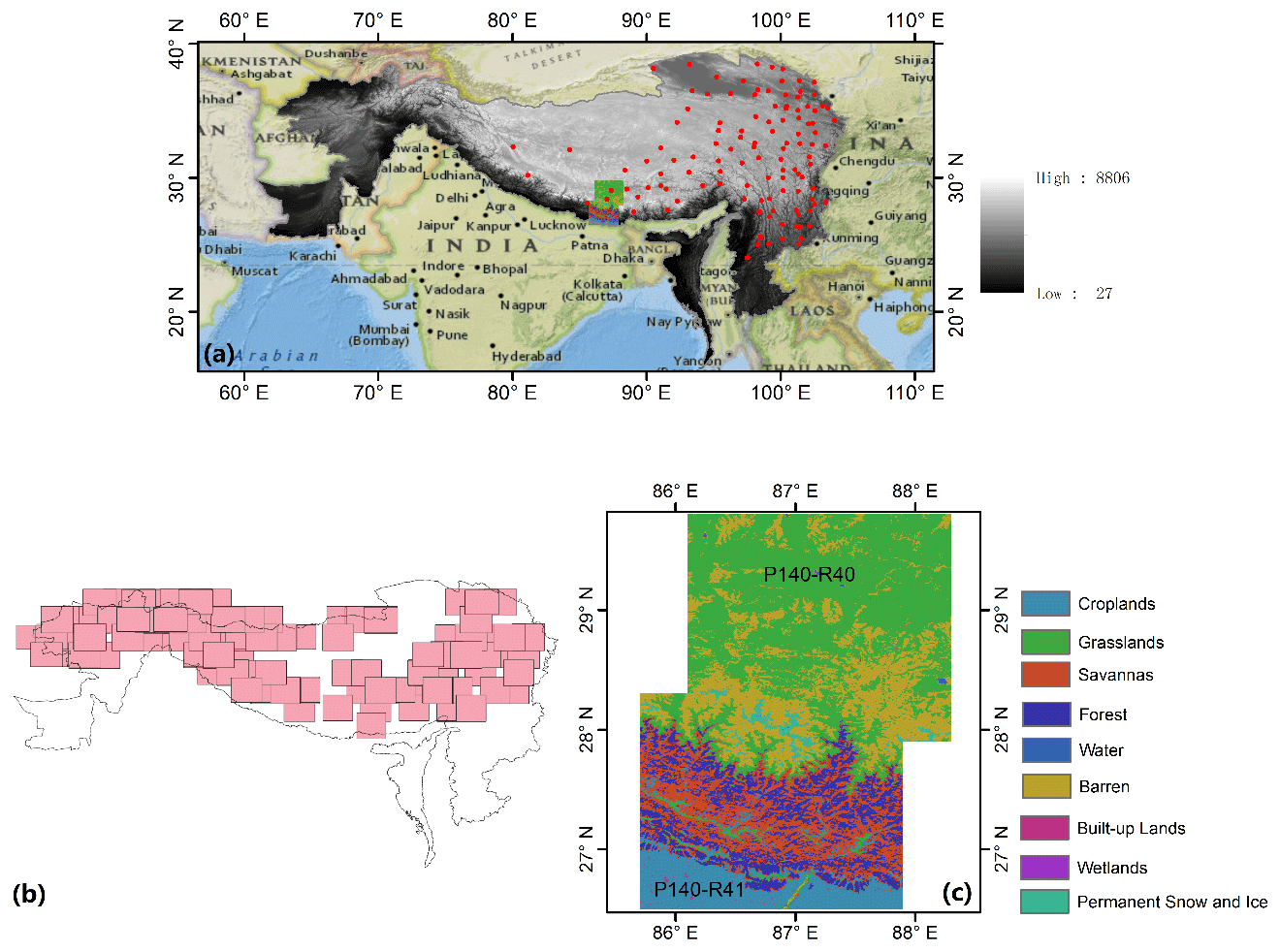
Figure 1(a) The HKH region and the distribution of in situ station locations (red dots). (b) The distribution of Landsat scenes available over the whole HKH region. (c) Land-cover type of the P140-R40/41 region of interest which corresponds to Landsat path 140, rows 41 and 42, on the Nepal–Tibet border.
2.2 AVHRR GAC snow extent retrieval
The AVHRR GAC snow-cover extent time series version 1 derived in the frame of the ESA CCI+ Snow project is the most recent long-term global snow-cover product available (Naegeli et al., 2021). It covers the period 1982–2019 at a daily temporal and 0.05∘ spatial resolution. The product is based on the Fundamental Climate Data Record (FCDR) consisting of daily composites of AVHRR GAC data (https://doi.org/10.5676/DWD/ESA_Cloud_cci/AVHRR-PM/V003) produced in the ESA CCI Cloud project (Stengel et al., 2020). The data were preprocessed with an improved geocoding and an inter-channel and inter-sensor calibration using PyGAC (Devasthale et al., 2017). The snow-cover extent retrieval method was developed and improved based on the ESA GlobSnow approach described by Metsämäki et al. (2015) and complemented with a pre-classification module. Alongside the daily reflectance and brightness temperature information, an excellent cloud mask including pixel-based uncertainty information is provided (Stengel et al., 2017, 2020). All cloud-free pixels are then used for the snow extent mapping using spectral bands centered at about 630 nm and 1.61 µm (channel 3a or the reflective part of channel 3b) and an emissive band centered at about 10.8 µm. The water bodies, permanent ice bodies, and missing values are flagged. SCAmod retrieves both the snow cover on top of the canopy, as well as on ground below the canopy, by taking the canopy density into account. Here, we focus on the latter variable as this is most suitable for the comparison with in situ stations.
To reduce the effect of cloud coverage, a temporal filter of ±3 d for each individual snow-cover observation was applied based on Foppa and Seiz (2012). The AVHRR GAC FCDR snow-cover product comprises only one longer data gap of 92 d between November 1994 and January 1995, resulting in a 99 % data coverage over the entire study period of 38 years. In this study, we will focus on the evaluation of raw daily retrieval of AVHRR GAC snow extent (denoted by “AVHRR_Raw”) since additional uncertainty will be introduced with the gap-filling process.
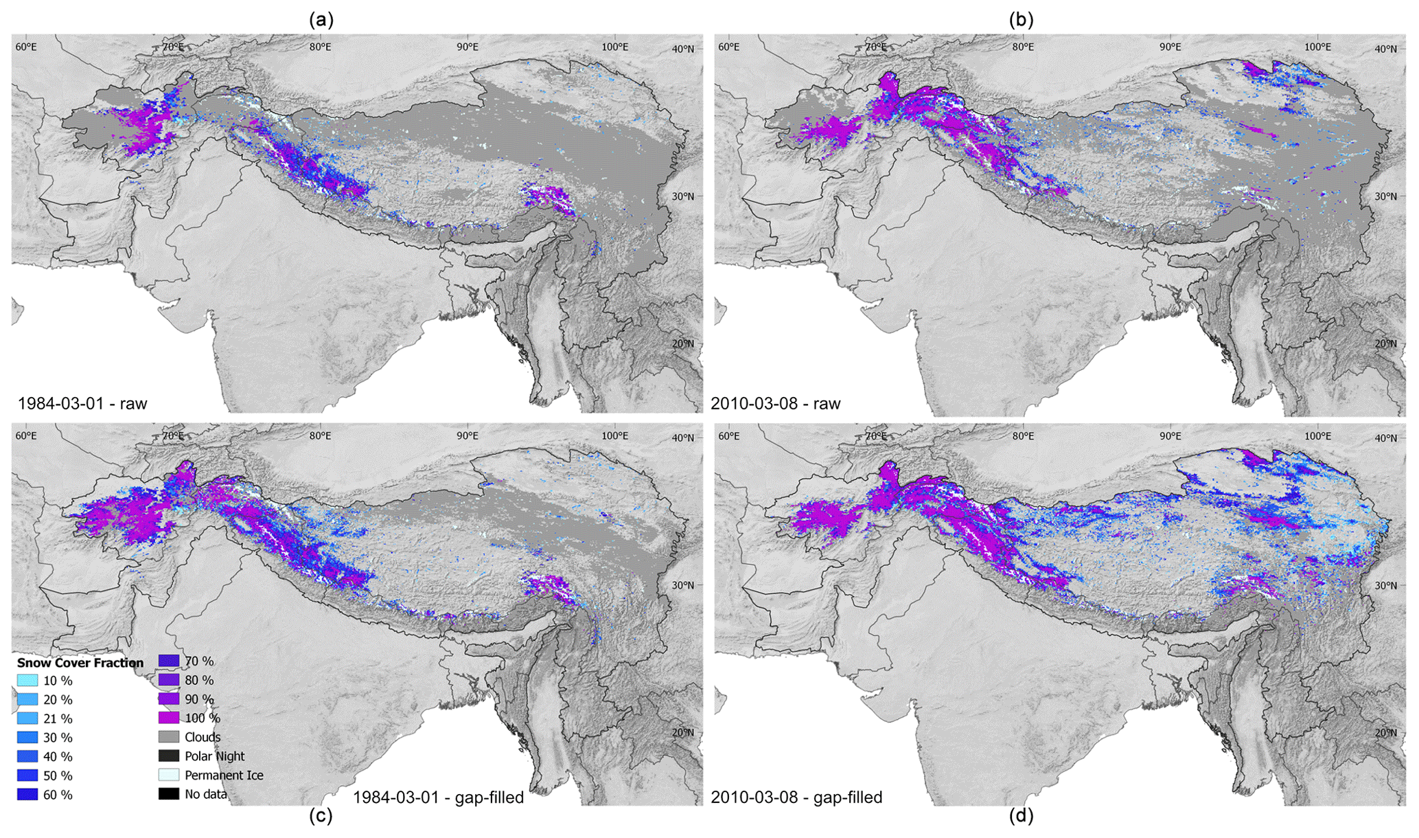
Figure 2AVHRR GAC raw (a, b) and gap-filled (c, d) snow cover for the entire HKH region in March 1984 (a, c) and March 2010 (b, d).
2.3 Validation datasets
2.3.1 In situ snow depth measurements
In situ data were provided by the China Meteorological Administration (https://data.cma.cn/en, last access: 30 October 2019). Daily snow depth (SD) measurements (118⋅365) are obtained from 118 stations located at different elevations ranging from 776 to 8530 m above sea level. SD was usually measured over a large flat area using rulers at 08:00 LT (UTC+8) every day. Three measurements were made at least 10 m away, and their mathematical mean was used as the daily snow depth. In particular, if snowfall occurred after 08:00, a second measurement at 14:00 or a third measurement at 20:00 were needed depending on the time of snowfall. The data were rounded to the nearest centimeter. Thus, SD less than 0.5 cm would be labeled as 0 cm in the record. Detailed quality control was made to flag suspicious values. The period from 1982 to 2013 was used to prove the temporal consistency of the AVHRR GAC snow-cover extent product.
2.3.2 Landsat TM/ETM data and processing
Landsat data were introduced for two purposes: (i) to check the spatial consistency between AVHRR GAC snow and Landsat-based snow based on 197 scenes covering the whole HKH region and (ii) to explore the factors (e.g., elevation, topography, and land cover) influencing the accuracy of AVHRR GAC snow based on P140-R40/41. To mitigate the effect of clouds, the validation over P140-R40/41 was restricted to clear-sky (cloud no more than 10 %) scenes of Landsat 5 TM during snow seasons (46⋅2 scenes from 1984 until 2013; downloaded from https://glovis.usgs.gov/, last access: 30 April 2020). The validation over the whole HKH region was restricted to Landsat clear-sky scenes from 1999 to 2018 (197 scenes) (Fig. 1b). Level-1 Precision and Terrain Correction (L1TP) data were selected since they have been radiometrically and geometrically corrected. Following the recommendation of Metsämäki et al. (2015), the fractional snow method by Salomonson and Appel (2006) was employed to generate reference FSC (fractional snow cover) from Landsat TM/ETM imagery. This method is originally designed for MODIS FSC products, with a mean absolute error of less than 10 % (Salomonson and Appel, 2004). In this paper, we assumed that such an accuracy can be achieved with higher resolution data. Bands 2 (0.53–0.61 µm) and 5 (1.55–1.75 µm) were used to provide NDSI (normalized difference snow index) estimates (Eq. 1), and then the Salomonson and Appel scaling (Eq. 2) is applied. These high-resolution data were then projected to a geographic projection and aggregated to AVHRR GAC pixel scale using the area-weighted average of contributing pixels to “simulate” the reference FSC estimates at the AVHRR GAC pixel scale.
where B2 and B5 denote the spectral bands 2 and 5, respectively.
2.3.3 MODIS snow-cover product
The Terra MODIS Level 3, Collection 6, 500 m daily snow-cover products (MOD10A1) (Hall and Riggs, 2016) over the HKH region from 2000 to 2013 were obtained through Google Earth Engine (GEE). The MODIS snow detection algorithm also uses NDSI and other test criteria (Riggs et al., 2016a). Instead of directly providing binary snow-covered area (SCA) and FSC, version V006 provides NDSI_Snow_Cover and NDSI. The former is reported in the range of 0–100 with other features identified by mask values, while the latter represents the real NDSI values multiplied by 10 000, which is calculated for all pixels (Riggs et al., 2016a). This treatment provides more information and great flexibility to enhance the accuracy of the product because the NDSI range is not necessarily restricted to 0.4 to 1.0 for snow detection. Actually, NDSI_Snow_Cover functions very similarly to FSC in version V005 since it can be linked using the equation of FSC . Compared to the previous version, version V006 made great improvements on atmospheric correction, cloud cover, and quality index. Furthermore, the algorithm takes a pixel's elevation into account, which is especially important for elevated snow-covered surfaces in spring. In order to avoid a spatial-scale mismatch between AVHRR and MODIS pixels, MOD10A1 was reprojected to a geographic projection and aggregated to AVHRR GAC pixel scale using the area-weighted average of contributing pixels.
2.3.4 Auxiliary data
The digital elevation model (DEM) information was obtained from the SRTM (Shuttle Radar Topography Mission) dataset, which provides a nearly global coverage with a spatial resolution of 90 m. In this study, the elevation, slope, aspect, and topographical variability were derived using this dataset in order to investigate their influences on the accuracy of the AVHRR GAC snow extent product. The topographical variability within a certain AVHRR GAC pixel was determined by calculating the standard deviation of elevations of all sub-pixels within its spatial extent, while the elevation, slope, and aspect were resampled to match the resolution of the AVHRR GAC snow dataset.
The MODIS Terra/Aqua Combined Annual Level 3 Global 500 m Collection 6 land-cover dataset (MCD12Q1) was generated using a supervised classification methodology (Friedl et al., 2010). In this study, the International Geosphere–Biosphere Programme (IGBP) of the MCD12Q1 mosaic was used to investigate the difference in accuracy over different land-cover types. It includes 11 types of natural vegetation, 3 types of developed and mosaic lands, and 3 types of non-vegetated lands, which have been reclassified into nine major classes: forest, grassland, savannas, croplands, built-up lands, barren, permanent snow and ice, water body, and wetlands. In order to match with the pixel size of AVHRR GAC snow, the MCD12Q1 was resampled to 0.05∘ spatial resolution with the nearest neighbor interpolation.
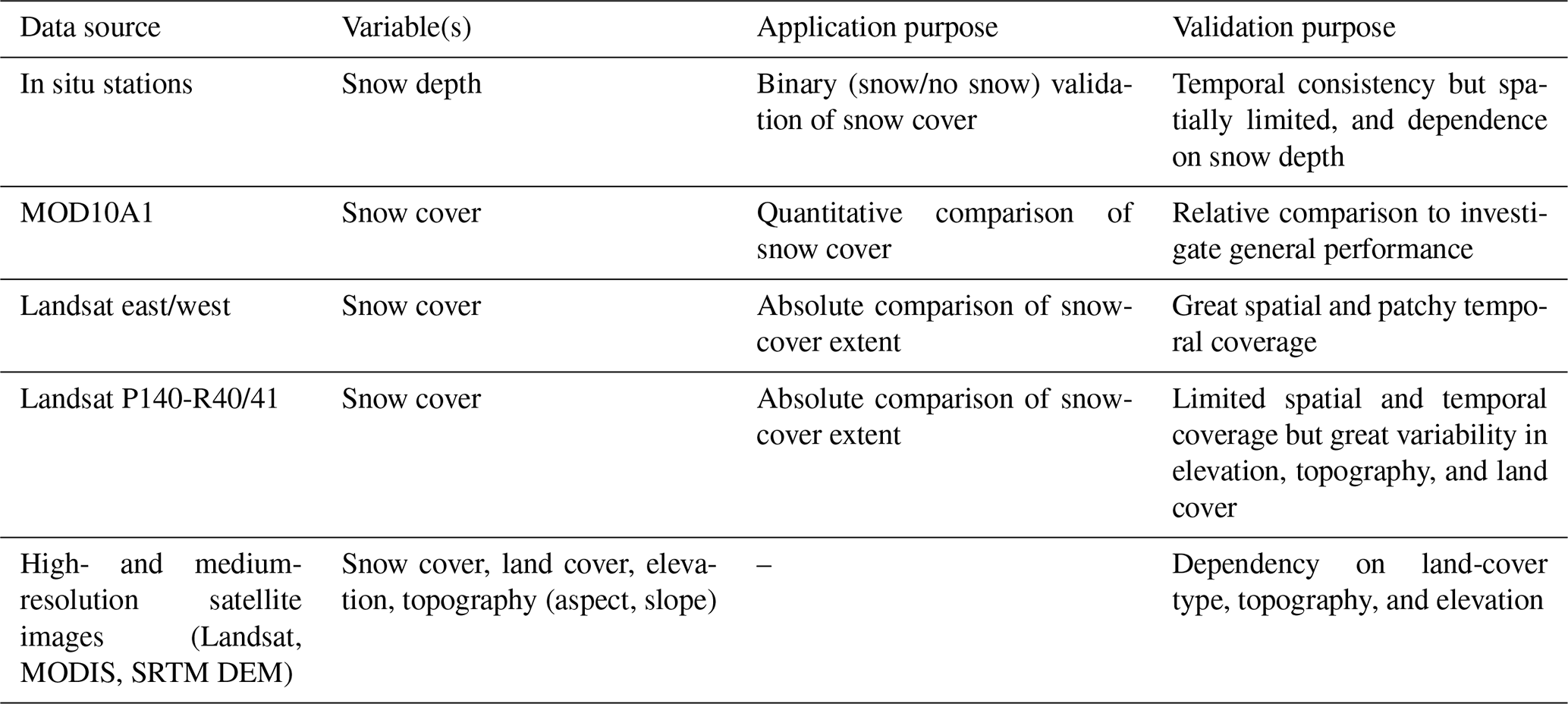
AVHRR GAC snow extent was evaluated from several aspects. The validation based on in situ sites aims to prove the long-term consistency since in situ stations provide valuable long time series measurements, while the comparison with Landsat and MODIS snow is focused on their spatial consistency and the in-depth analysis of influential factors (elevation, topography, and land cover). The validation strategy is briefly summarized in Table 1.
3.1 Binary validation based on in situ data
Although the validation based on in situ sites leaves issues of scale unresolved and therefore likely accompanied by uncertainties, in situ observations provide the only source to validate the time series AVHRR GAC snow extent over this long period. Since there is no reliable way to convert SD to FSC, both FSC and SD information were converted to binary information by applying appropriate thresholds, respectively. Different thresholds have been suggested for in situ SD measurements to determine whether the associated pixel is covered by snow, ranging from 0 to 5 cm (Parajka et al., 2012; Hori et al., 2017; Hao et al., 2019; Huang et al., 2018; Liu et al., 2018; Zhang et al., 2019; Gascoin et al., 2019). Therefore, the sensitivity of thresholds was tested by computing accuracy metrics with SD increasing from 1 to 5 cm. The FSC maps were transferred from fractional to binary snow information by applying a threshold of FSC ≥ 50 %. The value of 50 % is widely used and accepted in snow-cover detection (Wunderle et al., 2016; Mir et al., 2015; Crawford, 2015; Marchane et al., 2015; Hall and Riggs, 2007).
Concerning the comparison of spatial satellite data with in situ measurements, a point-wise comparison was implemented. To relate in situ “point” measurements with AVHRR GAC “area” snow information, both the center pixel containing the in situ point measurement and the 3×3 pixels centered around this point were tested, respectively. This treatment took into consideration the influence of data noise, geometric mismatch, and spatial heterogeneity. Furthermore, the absence or presence of snow indicated by in situ observations is assumed to be representative of at least a 3×3 pixel area, but this depends on topography. Consequently, there are altogether 10 combination cases for accuracy assessment (Table 2).

The 2×2 contingency table statistics (Table 3) were utilized to indicate the quality of the snow product. If both reference data and the snow product identified the pixel as snow, it is labeled as a hit (a); if neither of them indicated the pixel as snow, it is labeled as zero (d); if the snow product indicates the pixel as snow, but the reference data does not, it is marked as false (b); and if the opposite occurs, it is indicated as a miss (c) (Hüsler et al., 2012; Siljamo et al., 2011).
Table 3Contingency table used to determine probability of detection and bias.

Based on these measures, indicators such as accuracy (ACC), Heidke skill score (HSS), and bias (Bias) were determined (Eqs. 3–5) (Hüsler et al., 2012). ACC denotes the percentage of correctly classified pixels divided by the total number of pixels. ACC values closer to 1 denotes a perfect agreement between the snow product and the reference data, while a value of 0 corresponds to complete disagreement. However, it is strongly influenced by the most frequent category (i.e., in summer) (Hüsler et al., 2012) and thus ideally requires an equal distribution of categories. Hence, we confine our accuracy assessment to the snow season (from October to March) only, a limitation that was implemented in other studies as well (Yang et al., 2015; Gafurov et al., 2012; Hüsler et al., 2012; Huang et al., 2011). The HSS and Bias provide refined measures in cases when the frequency distribution within the validation subsets is not equal. The former describes the proportion of pixels correctly classified over the number that was correct by chance in the total absence of skill. Negative values indicate that the chance performance is better, 0 represents no skill, and a perfect performance obtains an HSS of 1 (Hüsler et al., 2012). It is generally true that a value above 0.3 denotes a relatively good score for a reasonably sized sample for the binary forecast (Singh, 2015). The Bias, described by the ratio of the number of snow-covered pixels to the number of reference data pixels, is a relative measure to detect overestimation (value is higher than 1) or underestimation of snow (value is less than 1). Unbiased results should have a value of 1.
The validation follows two types of strategies. First, the snow-cover data time series of satellite and in situ station were compared, resulting in accuracy indicators over each station. This validation allows us to check the spatial divergence of accuracy within different sites, as well as the effect of land cover on the accuracy of satellite-derived snow information. Second, the snow data of all in situ sites were combined together for validation of AVHRR GAC snow on the daily basis. In this way, the long-term temporal consistency of accuracy can be evaluated. Additionally, in order to assess the product performance with respect to the temporal variability in snow cover, the binary metrics are summarized and analyzed for each month. An analysis of increase/decrease in accuracy with respect to FSC and SD was also included to explore the influence of smaller snow patches on the accuracy.
Finally, in order to check the relative performance of AVHRR GAC snow to the well-used MODIS product, MOD10A1 V006 was also evaluated with in situ station data following the same method. It is expected that the major difference in their performance is either due to the quality of the applied processing and snow-cover retrieval algorithms or the general satellite data characteristics. As for the comparison of their absolute values, the root mean square error (RMSE), mean bias (mBias), and the coefficient of correlation (R) were derived through the scene-by-scene comparison.
3.2 Multi-scale validation based on high-resolution snow-cover maps
In order to evaluate AVHRR GAC snow at a broader spatial scale, Landsat TM/ETM aggregated FSC was used as the reference. Snow-free values are treated as 0 % snow, and a fully snow-covered pixel is assigned 100 % snow. The validation was conducted from two aspects: (i) one is based on 197 scenes covering the whole HKH region in order to increase the spatial coverage of validation, and (ii) the other is based on 46⋅2 scenes over P140-R40/41 in order to make a detailed analysis of the factors (e.g., elevation, topography, and land cover) influencing the accuracy of the AVHRR snow dataset.
4.1 The validation based on in situ data
4.1.1 Snow depths and pixel threshold sensitivity analysis
To test the sensitivity of the in situ SD threshold for the snow-cover detection, the overall accuracy metrics were computed by combining data of all in situ sites throughout the study period (from 1982 to 2013 for the AVHRR-GAC-derived snow and from 2000 to 2013 for MOD10A1). The variations in Bias, ACC, and HSS with all the threshold combinations (Table 2) are shown in Fig. 3.
As shown in Fig. 3a, an SD threshold of 2 cm (case2) maximizes the overall accuracy of the AVHRR GAC snow-cover dataset. With the further increase in SD threshold, the AVHRR GAC snow detected will be seriously overestimated. This indicates the presence of snow can be best detected by the AVHRR GAC dataset for in situ snow depth measurement of 2 cm. Furthermore, the increasing rate of ACC and decreasing rate of HSS are the highest between the 1 and 2 cm SD thresholds, and it flattens for greater SD thresholds. When it comes to the influences of geometric mismatch or spatial heterogeneity (center pixel versus 3×3 pixels; Table 2), they show significant effects on both the magnitude and the variation trend of these accuracy indicators. But such effects are not fixed and vary by satellite datasets and accuracy indicators (Fig. 3). For this reason, we chose case2 (SD ≥ 2 cm, center pixel) as the optimum threshold combination for the evaluation of the AVHRR GAC snow dataset. For consistency, this choice was also used for the comparison of the performance of MODIS with in situ data.
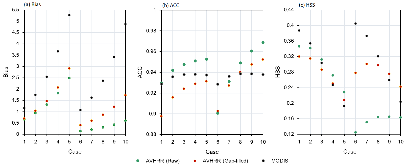
Figure 3Sensitivity analysis of product accuracy related to snow depth thresholds of the in situ station data. The overall error is a spatiotemporally integrated statistical measure.
As seen from Fig. 3a, AVHRR snow datasets show distinct advantages over MODIS snow regarding the Bias value. The former shows biases of 0.94 and 1.03 for the AVHRR raw snow and gap-filled snow, respectively, while the latter is seriously overestimated with the bias of 1.74. Nevertheless, the three datasets show comparable ACC, with the values of 0.94, 0.92, and 0.94 for AVHRR raw snow, AVHRR gap-filled snow, and MODIS snow datasets, respectively. The HSSs of the three datasets are reasonable, with the values larger than 0.3. MODIS snow shows the largest HSS of 0.35, followed by AVHRR raw snow with an HSS of 0.34. The AVHRR gap-filled snow-cover dataset ranks last, with the smallest HSS of 0.31. From the above results, it can be found that the AVHRR raw dataset performs slightly better than the AVHRR gap-filled dataset with respect to the agreement with in situ sites and the algorithm performance (skill). This is reasonable since additional uncertainty was introduced in the gap-filling process. For this reason, we will only focus on AVHRR raw snow for further analysis. Generally, AVHRR raw snow is comparable with MODIS snow when ACC and HSS are focused.
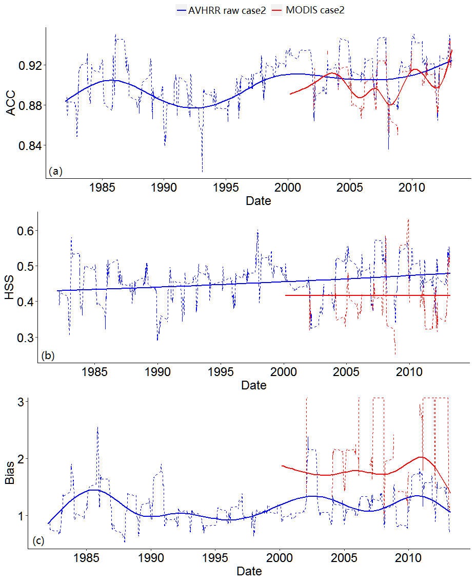
Figure 4The time series (denoted by the dashed lines) of ACC, HSS, and Bias for AVHRR raw and MODIS snow data during the investigated period. A simple moving average with a box dimension of n=30 was applied to the time series in order to reduce the noise and uncover patterns in the data. The solid lines represent the fitted trend of these accuracy indicators.
4.1.2 The temporal consistency of quality indicators
From Fig. 4, it can be seen that the interannual variability in these accuracy metrics is evident, especially for ACC and HSS. In the time series of AVHRR GAC snow, ACC is basically distributed between about 88 % and 92 % (Fig. 4a). An obvious increase in ACC can be observed from 1982 to 1985, followed by a decrease in ACC from 1985 to 1992. Then an increasing trend of ACC occurs from 1992 to 2000. From 2000 to 2010, ACC is relatively stable with time. But after 2010, an increasing trend reappears. Differently from the previous assessments, the ACC of the AVHRR snow datasets at the beginning of the time series (1982–2000) is slightly worse than the end of the time series (2000–2013) regarding the magnitude of ACC and its temporal consistency. The HSS shows a different behavior compared to ACC (Fig. 4b), which increases slightly and monotonously from 0.45 at the beginning to about 0.48 at the end of the time series. This further indicates that the performance of AVHRR snow continues to improve with time. Nevertheless, the improvements of the performance of AVHRR GAC snow do not occur in the Bias (Fig. 4c). The Bias shows the best performance from 1990 to 2000, with relatively stable values around 1. But during other time periods, relatively large fluctuations appear, and it generally overestimates snow during these periods.
As shown in Fig. 4, it can be seen that MODIS snow is inferior to AVHRR GAC snow regarding the magnitude of ACC and its temporal consistency. Furthermore, its HSS is consistently smaller than that of AVHRR GAC snow. Nevertheless, its temporal stability is slightly better than AVHRR GAC snow since the HSS of MODIS almost stays constant over time. When it comes to Bias, MODIS snow shows a more serious overestimation than AVHRR GAC snow but comparable temporal stabilities to the latter.
In order to highlight the performance of AVHRR GAC snow in different months, the temporal variations in ACC, HSS, and Bias over different months are presented (Fig. 5). From Fig. 5a, it can be seen that ACC of AVHRR GAC snow is over 0.85 for all months and even above 0.90 for October. Nevertheless, both the temporal variation trend and the magnitude of ACC show differences from month to month. It is clear that the AVHRR GAC snow shows the highest ACC in October and lowest ACC in January, but the temporal stability of ACC is best in November and worst in January and December. It is interesting that the results tend to polarize into two groups: ACC for January through March and ACC for October through December. Generally, ACC in the former group is smaller than those in the latter group. It is noteworthy that ACC after 2000 is generally larger and more stable than those in earlier years on the monthly scale (Fig. 5a), indicating the better accuracy and consistency of the younger satellite platforms after 2000. Compared to AVHRR GAC snow, the ACC of MODIS snow consistently shows large temporal variations for all months, and there is no month that shows advantages over others regarding the magnitude and temporal stability of ACC (Fig. 5b).
The HSS for different months are larger than 0.4 throughout the time series, but large differences of the magnitude and temporal stability exist between different months (Fig. 5c). Similar to ACC, the AVHRR GAC snow generally shows the largest HSS in October for most of the time. Furthermore, the HSS in October shows a similar temporal variation trend with the overall temporal trend of HSS in Fig. 4b. Among all the months, the HSS in December shows the largest temporal variations, featured by the highest HSS from 1990 to 2000 and the lowest HSS from 2005 to the end. The HSS in January through March shows relatively smaller temporal variations than those in October through December. Regarding the magnitude of HSS, the different rank of these months during different periods may be associated with the shift of snow-cover phenology due to interannual variability intensified by global warming. Unlike AVHRR GAC snow, MODIS snow shows larger HSSs in January and February (Fig. 5d). Furthermore, the temporal variations in HSS are more significant than AVHRR GAC during the same period.
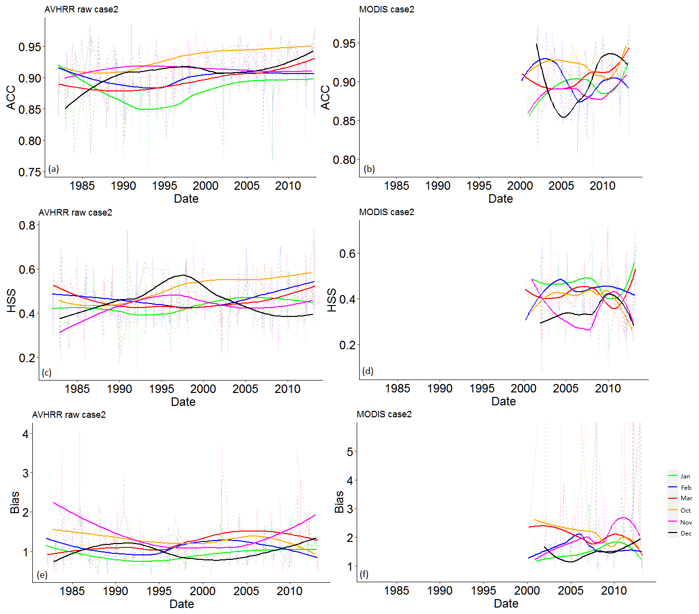
Figure 5The temporal behavior of ACC for AVHRR raw and MODIS snow data in different months (indicated by the different colored lines) during the snow season. The solid-colored lines represent the fitted trend of these accuracy indicators for different months.
Although the AVHRR GAC snow shows the best performance in October regarding the magnitude of ACC and HSS, it shows serious overestimation in this month (Fig. 5e). In particular, AVHRR GAC snow generally overestimates snow in February, March, October, and November. By contrast, it either slightly overestimates or underestimates snow in December and January, with the bias distributed around 1. This result is understandable because during December and January, snow coverage tends to be dense and spatially continuous, which results in unbiased estimation. By contrast, during February, March, October, and November, snow cover tends to be patchy, and AVHRR GAC data are more able to detect snow than in situ point observations due to the large pixel coverage. MODIS snow consistently overestimates snow in different months and shows larger temporal variations than AVHRR GAC snow (Fig. 5f).
From the results above, it can be concluded that the AVHRR GAC snow dataset performs variably throughout the course of the year, which may be related to the different amounts of snow in the HKH region. Generally, the magnitudes of ACC and HSS are largest in October and smallest in January. But the temporal stability of ACC is best in November and worst in January and December, while that of HSS is worst in December. The results of Bias provide different perspectives for the performance of AVHRR GAC snow. It generally overestimates snow in February, March, October, and November. By contrast, unbiased estimation is likely to occur in December and January. Compared to AVHRR snow datasets, the interannual variability in ACC, HSS, and Bias of the MODIS snow product in different months is generally stronger (Fig. 5).
4.1.3 The spatial consistency of quality indicators
Figure 6 show the boxplots of the validation metric derived from each in situ station, with the aim of revealing their spatial variability. It can be observed that the spatial variability in these validation metrics widely exists given their dispersed distribution. The maximum of ACC even reaches 0.99 for the AVHRR snow datasets, while the minimum values are close to 0.76 (Fig. 6a). Similarly, HSS also shows a dispersed distribution for the AVHRR snow datasets. The AVHRR raw dataset ranges from 0.2 to 0.39 with min–max values of 0.01 to about 0.68 (Fig. 6b). Likewise, the bias is located around 0.51–1.6 with min–max values of 0.05 and 2.89 for the AVHRR dataset (Fig. 6c). These results are understandable because the performance of satellite snow datasets is affected by many factors. Despite the awareness of spatial variability in these validation metrics, the degree of variability depends on satellite datasets and metrics. The HSS and Bias of the MODIS snow dataset are more divergent than the AVHRR raw snow dataset (Fig. 6).
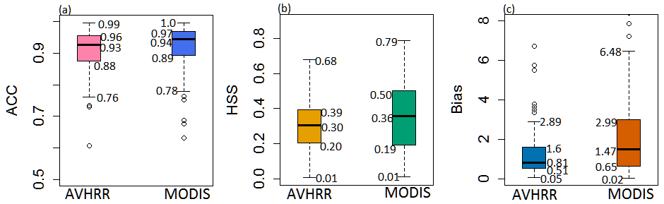
Figure 6The boxplots of ACC (a), HSS (b), and Bias (c) for AVHRR raw and MODIS snow data throughout the sites. The numbers around the plots indicate the minimum, lower quartile, median, upper quartile, and maximum of the boxplots.
4.1.4 The potential factors influencing accuracy
Following the early study (Klein and Barnett, 2003), the effect of SD on the accuracy of satellite snow datasets was evaluated (Fig. 7a). Observed SD was divided into six categories: SD = 0, 1, 2, 3, 4, and 5 cm. It is obvious that the ACC of the two satellite snow datasets based on AVHRR and MODIS show similar responses. The highest ACC occurred when SD=0 cm, which is followed by SD = 1 cm. When SD ≥ 2 cm, the ACC decreases significantly. The threshold of 2 cm which transforms in situ SD measurements to snow-cover or snow-free information is partly responsible for this result. Another cause of this phenomenon is the representativeness of the point-scale in situ observation compared with satellite observation on a larger pixel scale. When SD was less than 2 cm, it is more likely that snowfall events only occurred over a limited area of the satellite pixel. In this condition, satellite snow datasets are more likely to classify the pixel as snow-free, which would increase the agreement between satellite and in situ observations. Despite the decrease in ACC when SD ≥ 2 cm (compared to SD < 2 cm), the ACC of various snow datasets clearly shows an increasing trend with increasing SD. It is understandable since, with increasing SD, the satellite pixel is more likely to be entirely covered by snow, and the agreement between satellite and in situ observations, as a result, increases. In general, SD was shown to affect the overall agreement of satellite snow datasets, and their accuracies increase with increasing SD in the situation when the in situ site indicates snow-cover information, which is in line with previous studies (Zhou et al., 2013; Wang et al., 2009).
The effect of FSC on the accuracy of satellite snow datasets was checked in Fig. 7b. FSC was grouped into five categories using the ranges of 0 %–20 %, 20 %–40 %, 40 %–60 %, 60 %–80 %, and 80 %–100 %. Likewise, the ACC of the AVHRR and MODIS snow datasets shows a similar response to FSC. The highest ACC was found when FSC ≤ 20 %, followed by 20 % < FSC ≤ 40 %. This is also partly caused by the threshold (FSC ≥ 50 %) applied to FSC maps to transfer fractional to binary snow information and partly caused by the spatial representativeness of in situ sites. When only a small part of the pixel is covered by snow, in situ sites are more likely covered by very thin snow or not covered by snow. Consequently, in situ sites are more likely to be indicated as snow-free, which increases the agreement between in situ and satellite observations. In the situation of 40 % < FSC ≤ 60 %, ACC decreases significantly. This occurs because part of the satellite data in this group indicates snow cover using the threshold FSC ≥ 50 %, but there appears a strong possibility that the in situ site is not covered by snow or only covered by very thin snow. For the case of 60 % < FSC ≤ 80 %, all satellite data in this group indicate snow cover, but there remains a very real risk that the in situ site is not covered by snow or only covered by very thin snow. As a result, the agreement between them further decreases. With the further increase in FSC, the possibility that in situ sites indicate snow cover also increases. Thus, ACC increases in the situation of 80 % < FSC ≤ 100. From these results, it is concluded that FSC affects the overall agreement between satellite snow datasets and in situ observations. In the condition that satellite data indicate snow-free, ACC decreases with increasing FSC. By contrast, in the case of satellite data indicating snow cover, ACC increases with increasing FSC. Nevertheless, it is important to note that the variations in ACC with snow depth and FSC are related to the threshold adopted for transferring SD and FSC to snow-cover or snow-free information.

Figure 7The variation in ACC with snow depth (a) and FSC (b) for AVHRR raw and MODIS snow data throughout the sites during the experimental period.
As seen in Fig. 7a, we can find that the accuracy of the AVHRR snow datasets is larger than the MODIS snow product when SD ≤ 1 cm but consistently smaller than MODIS snow at each SD when SD ≥ 2 cm. This means that in snow-free or very thin snow conditions, the AVHRR snow datasets are less misclassified than the MODIS snow product, but in contrast, in snow-covered conditions, although the three datasets all reveal an increase in ACC with increasing SD, the MODIS snow product is more reliable and correctly classified. The discrepancies between them mainly result from the different spatial scale of the pixel. From Fig. 7b, it becomes apparent that accuracies of the AVHRR snow datasets are slightly lower than the MODIS product for each level of FSC when FSC ≤ 60 % but larger than the MODIS product when FSC > 60 %. This phenomenon is related to the different degrees of spatial representativeness of in situ sites relative to different pixel scales.
Figure 8a and b present the distribution of ACC for two satellite snow datasets against in situ site observations over different elevation regions (five classes) and land-cover types (four types), respectively. It is generally thought that coarse-pixel satellite snow products perform better at higher elevations due to the continuous and thick snow cover (Yang et al., 2011). Nevertheless, the ACC over the HKH region shows different phenomena. The two satellite snow products consistently show larger ACC over slightly lower elevations than those over higher elevations. Nevertheless, an exception can be found in the elevation region of 3500–4500 m, where the ACC of the two datasets is the lowest over the whole HKH region. Furthermore, the ACC over these elevation regions is the most divergent, demonstrating that the accuracy of snow product within this range is more likely to be affected by other factors. It is noteworthy that the MODIS snow product slightly outperforms the AVHRR snow dataset over different elevation regions. This is reasonable since the spatial-scale mismatch between in situ and satellite-based observations is greater for the AVHRR snow datasets than for the MODIS snow dataset.

Figure 8Boxplots of ACC from the direct comparison with in situ site observations over different elevation regions (a) and land-cover types (b) for AVHRR raw and MODIS snow data.
Despite the effect of elevation on ACC, it was not treated when we explored the effect of land-cover type on ACC (Fig. 8b) because the number of in situ sites over different land-cover types and different elevation regions are very limited. For AVHRR GAC snow, the highest agreement with in situ measurements is found in the barren class, followed by grasslands and savannas. Although nearly half of the in situ sites over forest show ACC larger than 0.91, substantial numbers of in situ stations show relatively low ACC over forest. This indicates that the well-known issues of identifying snow in forested areas using optical satellite data are not fully resolved in AVHRR GAC snow. It is interesting to find that the MODIS snow product maintains its superiority over different land-cover types, and its advantage becomes more pronounced over forest and savannas. The different performance between AVHRR snow and MODIS snow is partly caused by their individual accuracy and partly caused by the different effects of spatial-scale mismatch between in situ and satellite-based observations.
4.2 Comparison based on medium- to high-resolution data
4.2.1 Quantitative comparison to MOD10A1
In order to investigate the absolute difference between AVHRR GAC and MODIS snow, we compared them on the pixel basis following the cross-validation framework. The indicators of RMSE, mean Bias (mBias), and correlation coefficient (R) are used to reveal their differences and consistencies. The scene-by-scene comparison was made over the region P140-R40/41 throughout the snow season of 2012 and 2013. As shown in Fig. 9, the highest density is between 0 and −5 for mBias and 0 and 10 for RMSE. Only a small part of the scenes show a relatively large mBias of 15 % and RMSE of 30 %. Their overall mBias values are very small, with the values of 0.06 % and 0.94 % for the AVHRR raw and gap-filled snow datasets, respectively. The overall RMSEs are 12.8 % and 17.0 % for the AVHRR raw and gap-filled snow datasets, respectively. Furthermore, the spatial distribution characteristics of FSC indicated by AVHRR GAC snow basically agree with those of MODIS snow, given the overall R is 0.63 and 0.53 for the AVHRR raw and gap-filled snow datasets, respectively.
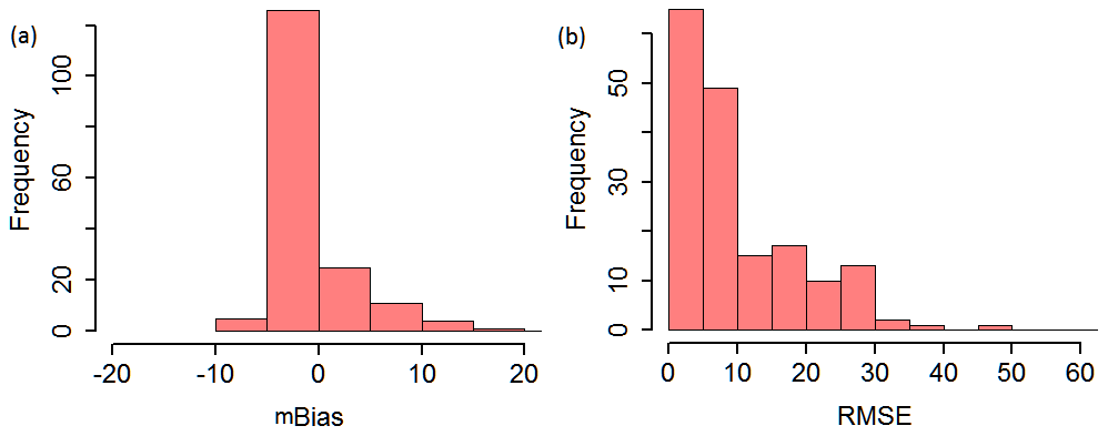
Figure 9The distribution of mBias (a) and RMSE (b) derived from the scene-by-scene comparison between the AVHRR GAC raw snow datasets and the MODIS snow products over the region P140-R40/41 throughout the snow season between 2012 and 2013.
4.2.2 Spatial consistency of snow-cover extent
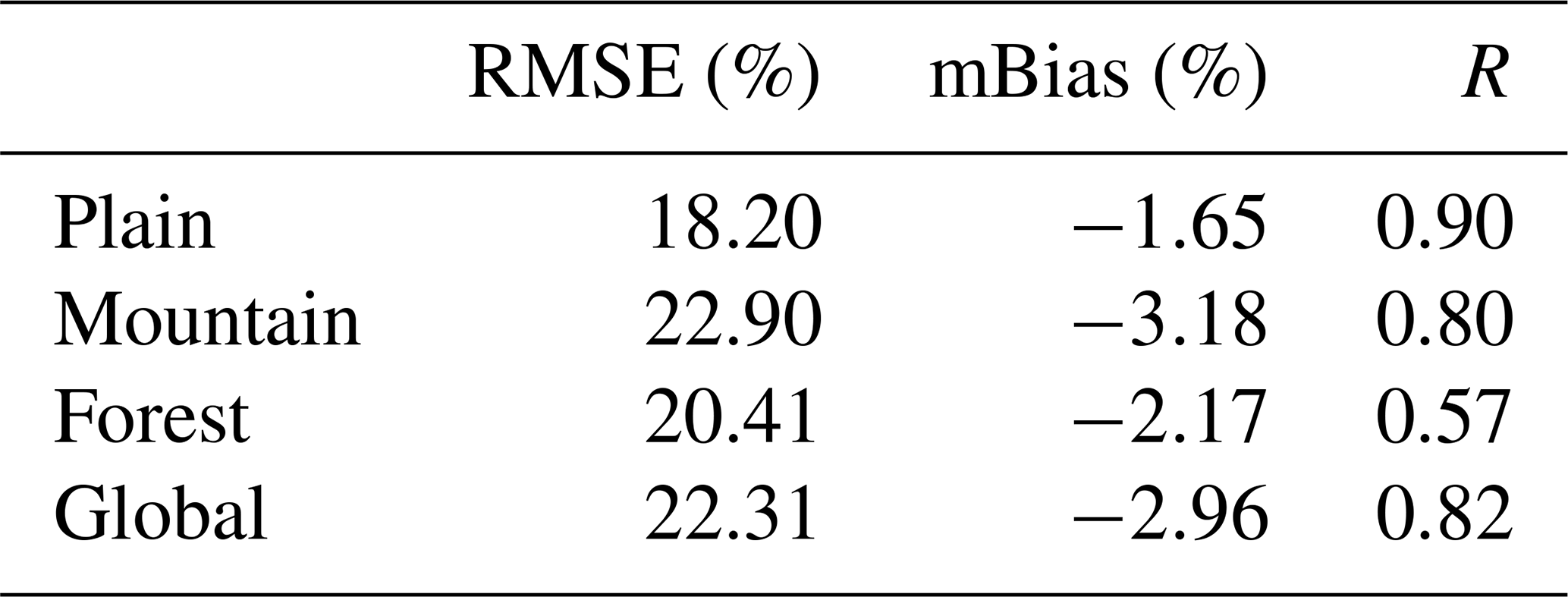
In order to avoid the spatial limitations of the in situ stations, the comparison between the AVHRR raw snow datasets and Landsat data was also carried out over the whole extent of the HKH region. The RMSE, mBias, and R in different conditions are summarized in Table 4. RMSE is generally less than 23 % in different conditions with an overall RMSE of 22.31 %. The mBias still indicates an underestimation of the AVHRR snow datasets, with the overall mBias of −2.96 %. The consistency between Landsat and AVHRR snow is good, with the overall R of 0.82. The best performance of AVHRR GAC snow is observed in the plain class, with the smallest RMSE of 18.2 % and mBias of −1.65, as well as the largest R of 0.90. By contrast, the largest RMSE of 22.9 % and mBias of −3.18 % appear in mountain areas. When it comes to consistency, the worst performance occurs in forests, with the lowest R of 0.57.
Table 4Summary of accuracies of AVHRR raw snow data with Landsat5 TM snow data over the whole HKH region.
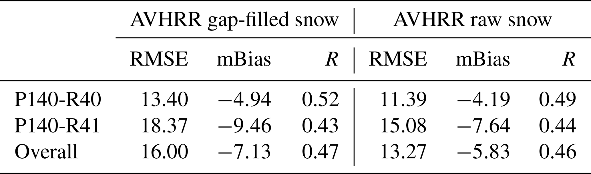
In order to explore the performance of AVHRR GAC snow in high detail for a wide range of conditions, the spatial accuracy was assessed on the pixel basis based on Landsat5 TM data time series over the areas covered by P140-R40/41. The AVHRR snow datasets systematically underestimate snow-covered areas with regards to the Landsat5 TM data (Table 5). This can be explained by the fact that direct coarse-resolution FSC is more likely to be lower than the FSC aggregated from high-resolution FSC because high-resolution data are able to pick up snow in one pixel, which is too little to create enough snow signals in coarse-resolution pixels but will show up in the aggregated FSC (Singh et al., 2014; Jain et al., 2008). The accuracy of AVHRR GAC snow is different over the two areas, with better performance over P140-R40 than P140-R41 (Table 5). AVHRR raw snow shows a higher accuracy with a smaller RMSE of 11.39 % (vs. 15.08 %) and mBias of −4.19 % (vs. −7.64 %) over P140-R40 than P140-R41. Similar results can also be seen in AVHRR gap-filled snow, with a smaller RMSE of 13.40 % (vs. 18.37 %) and mBias of −4.94 % (vs. −9.46 %) over P140-R40 than P140-R41. When the two areas are combined together, the AVHRR GAC snow presents overall RMSEs of 13.27 % and 16 % and mBias values of −5.83 % and −7.13 % for the raw and gap-filled datasets, respectively, over the highly variable region (e.g., elevation, topography, and land cover). From Table 5, it is clear that AVHRR raw snow shows a higher accuracy than the gap-filled snow dataset. But their overall consistency with Landsat TM snow is comparable (0.46 and 0.47 for raw and gap-filled snow datasets).
Table 5Summary of accuracies of AVHRR raw and AVHRR gap-filled snow data with Landsat5 TM snow over P140-R40 and P140-R41.
4.2.3 Pixel-based comparison and potential factors influencing accuracy
Both the land-cover types and topographies are highly heterogeneous over the HKH region. Here, the sub-region P140-R40/41 was chosen to investigate the factors (i.e., elevations, land-cover type, slope, aspect, and topographical variability) influencing the accuracy of the AVHRR GAC snow dataset (Fig. 10). From Fig. 10a, it can be seen that RMSE shows a strong positive response to elevations. But an exception can be found within the region of 3500–4500 m, where RMSE shows a clear decrease but also the greatest spread. This occurs because the accuracy of AVHRR GAC snow is not merely influenced by elevations. Over the flat areas (0–200 m) and hills (200–500 m), the highest density of RMSEs is distributed between 0 % and 5 %. Over lower and medium height mountains (500–2500 m), the highest density of RMSEs is distributed between 0 % and 10 %. With the further increase in elevation (i.e., 2500–3500 m), more than half of the pixels show RMSEs larger than 10 %. Nevertheless, over the elevation region of 3500–4500 m, more than half of the pixels show small RMSEs of less than 5 %. But the maximum RMSE can reach 45 % over this region. Over the elevation region of 3500–4500 m, the highest density of RMSEs is lower than 15 %, and the RMSE increases significantly over the extreme high area (>5500 m). This finding is inconsistent with Yang et al. (2011) who consider that coarse-pixel satellite snow products generally perform better at higher elevations due to the continuous and thick snow cover. The larger RMSEs in the highest elevations are partly caused by the large values of FSC themselves, partly caused by the roughness, topographic effects, and shadows, and partly caused by the cloud effects given that the probability of cloud rises with rising altitude in mountain areas.
Given the considerable effect of elevation on the accuracy of AVHRR GAC snow, the regions P140-R40/41 are divided into eight groups according to their elevations (Fig. 10b). From Fig. 10b, it can be seen that the RMSE is rising with elevation in each individual land-cover type. Nevertheless, an exception can be found in grasslands, which show the largest RMSE over the region 2500–3500 m, and the RMSEs decrease significantly over the region 3500–4500 m. Over the flat areas (0–200 m), AVHRR snow mapping accuracy is the best in croplands and the worst in the barren class, and the accuracy is slightly better in forest than in savannas. Moreover, the accuracy is most spatially stable in grasslands given the centralized distribution of RMSE. When it comes to hills (200–500 m), croplands still show the best accuracy, followed by the forest and grasslands, and savannas rank last. As the elevation increases to 500–1500 m, croplands still show the best accuracy. By contrast, grasslands show the worst accuracy. Savannas show a smaller RMSE than forests. With the further increase in elevations (2500–3500 m), only grassland, savannas, and forests appear. The best performance occurs in forests, followed by savannas, and grasslands rank last. Over the high mountain area (3500–4500 m), savannas present the largest RMSE, followed by forest, and the grasslands show the largest spatial variations within this range. With the further increase in elevation (>4500 m), only grasslands and the barren class appear, and the former shows better accuracy than the latter with regard to the magnitude of RMSE and its spatial variations. Therefore, we can conclude that the performance of AVHRR GAC snow over different land-cover types depends mainly on elevations. Its accuracy is generally good in croplands since it is distributed only within the region of <1500 m. The accuracy of the barren class is generally not good because it is merely distributed within the range of >3500 m. Forests and savannas basically show comparable overall accuracy. The accuracy of grasslands shows a different response to elevations, which is the worst over regions of 2500–3500 m height. Its accuracy is comparable to other land-cover types over relatively low elevations (<1500 m) and outperforms the barren class over high elevations (>3500 m).
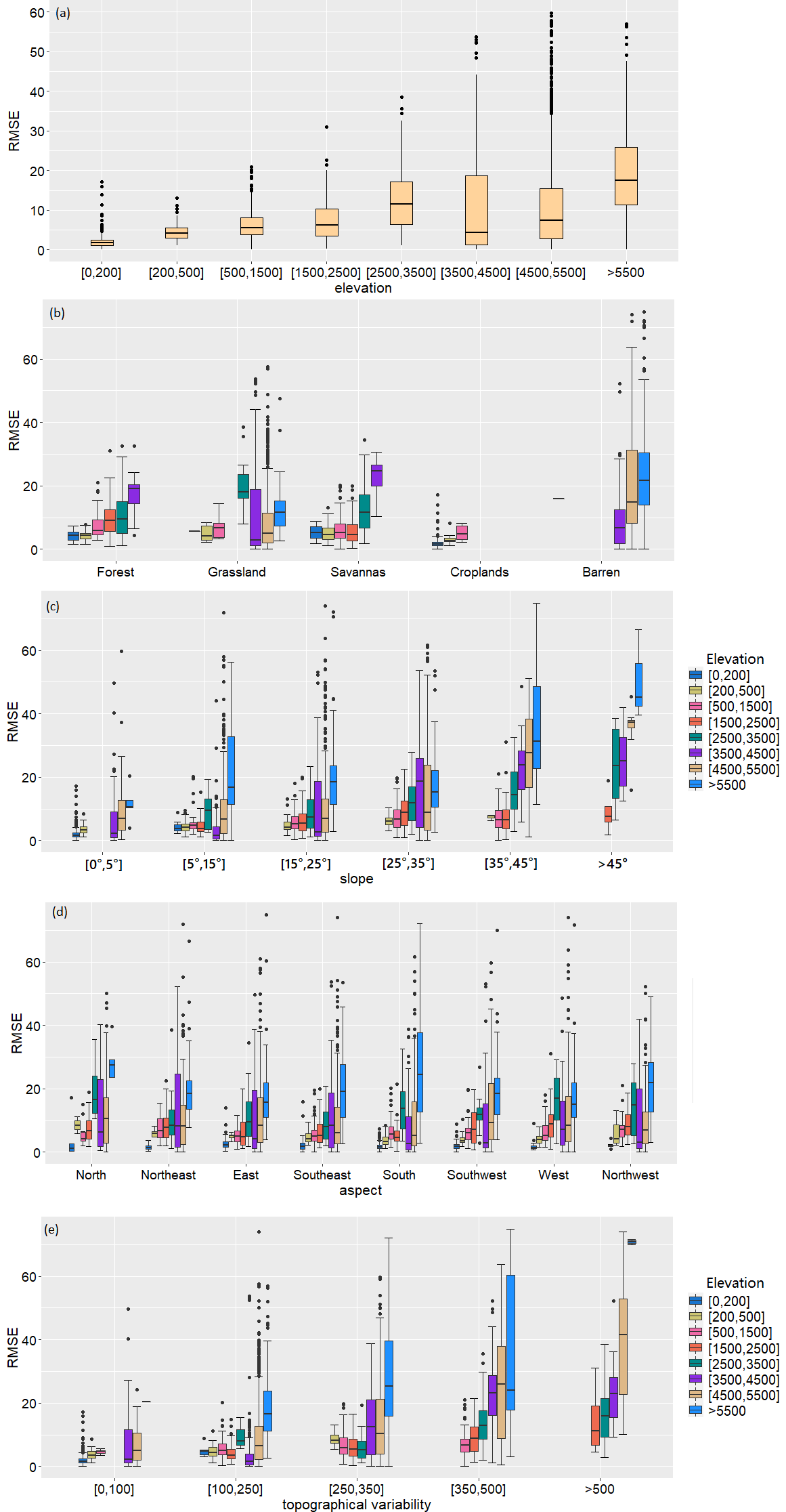
Figure 10The variations in RMSE dependent on (a) elevation, (b) land cover, (c) slope, (d) aspect, and (e) topographical variability. The different colors refer to the eight different elevation classes. The plots show combined results of P140-R40 and P140-R41.
The effect of slope on the accuracy of the AVHRR GAC snow datasets is clearly shown in Fig. 10c. Better results tend to appear over the areas with smaller slopes. The RMSE over different elevation regions generally shows an increasing trend with slope. Nevertheless, there are two outliers over the regions of 1500–2500 m and extremely high areas (>5000 m). In the former region, the RMSEs with slopes ranging from 25 to 35∘ are slightly larger than those with slopes ranging from 35 to 45∘. In the latter region, there is no increase in RMSE when slopes increase from 15–25∘ to 25–35∘. This occurs because the accuracy of AVHRR GAC snow is affected by many factors. In fact, the effect of slope on snow mapping accuracy is understandable since the topographic effects tend to be significant in a steep mountain area.
Regarding the effect of aspect (Fig. 10d), there is not a clear trend of RMSEs with aspect over the regions lower than 5000 m. Nevertheless, over the areas higher than 5500 m, the RMSEs first show a clear decreasing trend and then a clear increasing trend when aspect changes from the north-facing slope to the south-facing slope, and vice versa. Moreover, the maximum RMSE can even reach 70 % over the south-facing slope, which is larger than that of the north-facing slope (∼40 %). This is attributed to the fact that during winter months, the south-facing slopes receive significantly more radiant energy, providing an unfavorable environment for snow accumulation. Thus, snow cover on the south-facing slopes is more likely to be shallowness and patchiness, reducing the accuracy of the AVHRR GAC snow datasets.
From Fig. 10e, it can be found that there is only small topographical variability over the regions with low elevations (<500 m). The RMSEs of these regions with different elevations generally show an increasing trend with topographical variability, indicating its significant effect on the accuracy of the AVHRR GAC snow datasets. This is because the rugged relief can lead to shadowing effects, resulting in different degrees of surface information loss between high-resolution satellite data and coarse-resolution satellite data. Furthermore, the increasing trend is more significant over the regions with large elevations. It is noteworthy that there are also several outliers that do not show a clear increasing trend. For instance, over the elevation region of 2500–3500 m, even a decrease in RMSE can be observed when topographical variability increases from 100–250 to 250–350 m. This is due to the fact that the topographical variability is just one of the factors influencing the accuracy of AVHRR GAC snow.
From the results above, we can conclude that the accuracy of AVHRR GAC snow is closely related to elevations, slopes, and topographical variability, and the negative influence of these factors on snow mapping accuracy is more significant over regions with high elevations. The effect of aspect can be ignored over the regions lower than 5500 m, but for the areas higher than 5500 m, the accuracy first increases and then decreases gradually from the north-facing slope to the south-facing slope, and vice versa. The effect of land-cover type on snow mapping accuracy is related to elevations.
In this study, the ESA CCI+ Snow project AVHRR GAC snow-cover extent product was evaluated using different reference datasets. Compared to other AVHRR snow extent products, this dataset is designed to provide global snow extent with consistent performance across the whole suite of AVHRR sensors, which is considered a major step toward a detailed snow climatology on the global scale. The validation was conducted from two aspects. First, more than 30 years of in situ measurements over 118 stations were employed to assess the sensor-to-sensor consistency. Second, medium- to high-resolution data (i.e., MODIS and Landsat snow) were introduced to provide great spatial coverage and investigate the general performance of AVHRR GAC snow. Furthermore, an in-depth analysis was made over the area with a wide range of conditions (e.g., elevation, topography, and land cover) in order to explore the factors influencing the performance of AVHRR GAC snow.
Validated against in situ station observations, the overall ACC of the AVHRR raw snow dataset was about 94 %, which is the same as for MOD10A1. The use of a temporal filter caused a slight reduction in ACC of the AVHRR gap-filled snow dataset, with overall values around 92 %. AVHRR GAC raw snow is slightly underestimated, with the bias of 0.94. Based on the observations of all in situ sites, we obtain HSS = 0.34 for AVHRR GAC snow, which is also comparable to the one for MOD10A1 (HSS = 0.35). When validated against Landsat5 TM images over the whole HKH region, the RMSE and R are 22.31 % and 0.82, respectively, but for the highly variable sub-region P140-R40/41, AVHRR GAC snow presents RMSEs of 13.27 % and 16 % and mBias values of −5.83 % and −7.13 for the raw and gap-filled datasets, respectively. Their consistency with Landsat snow is reduced, with a relatively low R of 0.46 and 0.47 for raw and gap-filled snow datasets, respectively.
Regarding the temporal consistency of the AVHRR GAC snow datasets, the sensor-to-sensor consistency was found to differ slightly and unsystematically in ACC and Bias throughout the time series. While the consistent slight increasing trend of HSS is noteworthy, it is important to point out that the different performance of the AVHRR GAC snow datasets in different months is mainly caused by the variable amount of snow. Particularly, the performance of AVHRR GAC snow is worst in January and best in October regarding the magnitude of ACC and HSS, but when the temporal stability of accuracy was considered, it performs best in November and worst in January and December regarding the ACC, while that of HSS is worst in December. The results of Bias provide different perspectives for the performance of AVHRR GAC snow. It generally overestimates snow in February, March, October, and November, which is strongly linked to the patchiness of the snow cover that is not captured by the in situ data. By contrast, unbiased estimation is likely to occur in December and January when the snow cover is most continuous over greater areas.
The validation results with two independent reference datasets (i.e., in situ and Landsat) both show considerable spatial variabilities, indicating the effect of other factors (e.g., SD, FSC, land-cover type, elevation, slope, aspect, and topographical variability). Generally, in snow-covered situations, the accuracy of satellite snow datasets increases with increasing SD and FSC. By contrast, in snow-free conditions, accuracy decreases with increasing SD and FSC. Furthermore, the accuracy of AVHRR GAC snow is closely related to elevations, slopes, and topographical variability, and the negative influence of these factors on snow mapping accuracy is more significant over regions with high elevations. The RMSE over different elevation regions generally shows an increasing trend with slope. The effect of aspect can be ignored over the regions lower than 5500 m, but over the areas higher than 5500 m, the accuracy first increases and then decreases gradually from the north-facing slope to the south-facing slope, and vice versa. The effect of land-cover type on snow mapping accuracy is related to elevations. Its accuracy is generally good in croplands since it is distributed only within the region of <1500 m. The accuracy of the barren class is generally not good because it is merely distributed within the range of >3500 m. Forests and savannas basically show comparable overall accuracy. The accuracy of grasslands shows different responses to elevations, which is the worst over regions of 2500–3500 m height. Its accuracy is comparable to other land-cover types over relatively low elevations (<1500 m) and outperforms the barren class over high elevations (>3500 m).
When it comes to the performance relative to the MODIS snow products, AVHRR raw snow is comparable with MODIS snow when ACC and HSS are focused. Nevertheless, it shows distinct advantages over the MODIS snow product focusing on Bias. Regarding the temporal and spatial behaviors, different results appear in the two dimensions. In the temporal dimension, the AVHRR snow datasets display a more stable behavior regarding the ACC but less stable regarding the HSS than the MODIS snow products, but in the spatial dimension, the AVHRR snow datasets show a comparable spatial variability in accuracy but a smaller spatial variability in HSS and Bias than the MODIS snow products. The absolute differences between the AVHRR GAC and MODIS snow datasets were still reasonable, with the overall RMSE of 12.8 % and 17.0 %, mBias of 0.06 % and 0.94 %, and R of 0.63 and 0.53 for the AVHRR raw and gap-filled snow datasets, respectively.
This study represents the first validation of the unique daily AVHRR GAC snow extent spanning 4 decades over the HKH region.
Although the reference datasets (i.e., in situ sites, high-resolution satellite data) have their own limitations and flaws, our results still encourage the compilation of a consistent, complete, long time series snow extent dataset from historical AVHRR GAC data. This study characterizes the product performance with distinct accuracy parameters from different perspectives and thus contributes to the ongoing efforts to improve the performance of existing snow products by enhancing our knowledge of the thematic and absolute accuracy of current products.
The in situ snow depth data are provided by the China Meteorology Administration (CMA) (https://data.cma.cn/en, last access: 30 October 2019), which are not available to the public due to legal constraints on the data's availability. The Landsat Collection 1 Tier 1 data from Landsat 4 (https://doi.org/10.5066/F7N015TQ, USGS, 2020a) to Landsat 8 (https://doi.org/10.5066/F71835S6, USGS, 2020b) are publicly available via https://glovis.usgs.gov/ (last access: 30 April 2020). The MOD10A1 dataset is provided by NASA National Snow and Ice Data Center Distributed Active Archive Center (NSIDC DAAC), which is registered at https://doi.org/10.5067/MODIS/MOD10A1.006 (Hall and Riggs, 2016). It was downloaded using Google Earth Engine via the code presented at https://developers.google.com/earth-engine/datasets/catalog/MODIS_006_MOD10A1 (last access: 30 April 2020). The AVHRR GAC SCFG is openly accessible at https://doi.org/10.5285/5484dc1392bc43c1ace73ba38a22ac56 (Naegeli et al., 2021).
XW was responsible for the main research ideas and writing the manuscript. KN, VP, CM, DM, and JW contributed to the data collection. SW contributed to the manuscript organization. All the authors thoroughly reviewed and edited this paper.
The contact author has declared that neither they nor their co-authors have any competing interests.
Publisher's note: Copernicus Publications remains neutral with regard to jurisdictional claims in published maps and institutional affiliations.
The authors are grateful to the ESA CCI (Climate Change Initiative) cloud project team for making the datasets available for this study. The in situ data were provided by the China Meteorology Administration (CMA) (https://data.cma.cn/en, last access: 30 October 2019).
This research has been supported by the National Natural Science Foundation of China (grant no. 42071296). This work was jointly supported by the National Natural Science Foundation of China (grant no. 41801226) and the European Space Agency (ESA) Snow Climate Initiative (CCI+) project (grant no. 4000124098/18/I-NB).
This paper was edited by Alexandre Langlois and reviewed by three anonymous referees.
Anderson, K., Fawcett, D., Cugulliere, A., Benford, S., Jones, D., and Leng, R.: Vegetation expansion in the subnival Hindu Kush Himalaya, Glob. Chang Biol., 26, 1608–1625, https://doi.org/10.1111/gcb.14919, 2020.
Arsenault, K. R., Houser, P. R., and De Lannoy, G. J.: Evaluation of the MODIS snow cover fraction product, Hydrol. Process., 28, 980–998, 2014.
Bookhagen, B. and Burbank, D. W.: Topography, relief, and TRMM-derived rainfall variations along the Himalaya, Geophys. Res. Lett., 33, L08405, https://doi.org/10.1029/2006GL026037, 2006.
Brown, R. D. and Mote, P. W.: The response of Northern Hemisphere snow cover to a changing climate, J. Climate, 22, 2124–2145, 2009.
Crawford, C. J.: MODIS Terra Collection 6 fractional snow cover validation in mountainous terrain during spring snowmelt using Landsat TM and ETM+, Hydrol. Process., 29, 128–138, 2015.
Devasthale, A., Raspaud, M., Schlundt, C., Hanschmann, T., Finkensieper, S., Dybbroe, A., Hörnquist, S., Håkansson, N., Stengel, M., and Karlsson, K.: PyGac: An open-source, community-driven Python interface to preprocess nearly 40-year AVHRR Global Area Coverage (GAC) data record, Quarterly, 11, 3–5, 2017.
Fletcher, C. G., Kushner, P. J., Hall, A., and Qu, X.: Circulation responses to snow albedo feedback in climate change, Geophys. Res. Lett., 36, 1–4, 2009.
Foppa, N. and Seiz, G.: Inter-annual variations of snow days over Switzerland from 2000–2010 derived from MODIS satellite data, The Cryosphere, 6, 331–342, https://doi.org/10.5194/tc-6-331-2012, 2012.
Foster, J. L., Hall, D. K., Eylan De R, J. B., Riggs, G. A., Nghiem, S. V., and Te De Sco, M.: A blended global snow product using visible, passive microwave and scatterometer satellite data, Int. J. Remote S., 32, 1371–1395, 2011.
Friedl, M. A., Sulla-Menashe, D., Tan, B., Schneider, A., Ramankutty, N., Sibley, A., and Huang, X.: MODIS Collection 5 global land cover: Algorithm refinements and characterization of new datasets, Remote Sens. Environ., 114, 168–182, 2010.
Gafurov, A., Kriegel, D., Vorogushyn, S., and Merz, B.: Evaluation of remotely sensed snow cover product in Central Asia, Hydrol. Res., 44, 506–522, 2012.
Gascoin, S., Grizonnet, M., Bouchet, M., Salgues, G., and Hagolle, O.: Theia Snow collection: high-resolution operational snow cover maps from Sentinel-2 and Landsat-8 data, Earth Syst. Sci. Data, 11, 493–514, https://doi.org/10.5194/essd-11-493-2019, 2019.
Guangwei, C.: Summary reports of workshops on biodiversity conservation in the Hindu Kush-Himalayan ecoregion, in: Biodiversity in the eastern Himalayas: conservation through dialogue, ICIMOD, 2002.
Hall, D. K. and Riggs, G. A.: Accuracy assessment of the MODIS snow products, Hydrol. Process., 21, 1534–1547, 2007.
Hall, D. K. and Riggs, G. A.: MODIS/Terra Snow Cover Daily L3 Global 500m SIN Grid, Version 6. Boulder, Colorado USA, NASA National Snow and Ice Data Center Distributed Active Archive Center [data set], https://doi.org/10.5067/MODIS/MOD10A1.006, 2016.
Hao, S., Jiang, L., Shi, J., Wang, G., and Liu, X.: Assessment of modis-based fractional snow cover products over the tibetan plateau, IEEE J. Sel. Topics Appl. Earth Observ., PP, 1–16, 2018.
Hao, X., Luo, S., Che, T., Wang, J., Li, H., Dai, L., Huang, X., and Feng, Q.: Accuracy assessment of four cloud-free snow cover products over the Qinghai-Tibetan Plateau, Int. J. Digit. Earth, 12, 375–393, 2019.
Hori, M., Sugiura, K., Kobayashi, K., Aoki, T., Tanikawa, T., Kuchiki, K., Niwano, M., and Enomoto, H.: A 38-year (1978–2015) Northern Hemisphere daily snow cover extent product derived using consistent objective criteria from satellite-borne optical sensors, Remote Sens. Environ., 191, 402–418, 2017.
Hüsler, F., Jonas, T., Wunderle, S., and Albrecht, S.: Validation of a modified snow cover retrieval algorithm from historical 1-km AVHRR data over the European Alps, Remote Sens. Environ., 121, 497–515, 2012.
Huang, X., Liang, T., Zhang, X., and Guo, Z.: Validation of MODIS snow cover products using Landsat and ground measurements during the 2001–2005 snow seasons over northern Xinjiang, China, Int. J. Remote. Sens., 32, 133–152, 2011.
Huang, Y., Liu, H., Yu, B., Wu, J., Kang, E. L., Xu, M., Wang, S., Klein, A., and Chen, Y.: Improving MODIS snow products with a HMRF-based spatio-temporal modeling technique in the Upper Rio Grande Basin, Remote Sens. Environ., 204, 568–582, 2018.
Immerzeel, W. W., Droogers, P., Jong, S. M. D., and Bierkens, M.: Large-scale monitoring of snow cover and runoff simulation in himalayan river basins using remote sensing, Remote Sens. Environ., 113, 40–49, 2009.
IPCC: Climate Change 2013, The Physical Science Basic. Contribution of Working Group I to the Fifth Assessment Report of the Intergovernmental Panel on Climate Change, Cambridge University Press, Cambridge and New York, 2013.
Jain, S. K., Goswami, A., and Saraf, A. K.: Accuracy assessment of MODIS, NOAA and IRS data in snow cover mapping under Himalayan conditions, Int. J. Remote. Sens., 29, 5863–5878, 2008.
Klein, A. G. and Barnett, A. C.: Validation of daily modis snow cover maps of the upper rio grande river basin for the 2000–2001 snow year, Remote Sens. Environ., 86, 162–176, 2003.
Liu, X., Jiang, L., Wu, S., Hao, S., Wang, G., and Yang, J.: Assessment of methods for passive microwave snow cover mapping using FY-3C/MWRI data in China, Remote Sens., 10, 524, https://doi.org/10.3390/rs10040524, 2018.
Marchane, A., Jarlan, L., Hanich, L., Boudhar, A., Gascoin, S., Tavernier, A., Filali, N., Le Page, M., Hagolle, O., and Berjamy, B.: Assessment of daily MODIS snow cover products to monitor snow cover dynamics over the Moroccan Atlas mountain range, Remote Sens. Environ., 160, 72–86, 2015.
Metsämäki, S., Pulliainen, J., Salminen, M., Luojus, K., Wiesmann, A., Solberg, R., Böttcher, K., Hiltunen, M., and Ripper, E.: Introduction to globsnow snow extent products with considerations for accuracy assessment, Remote Sens. Environ., 156, 96–108, 2015.
Mir, R. A., Jain, S. K., Saraf, A. K., and Goswami, A.: Accuracy assessment and trend analysis of MODIS-derived data on snow-covered areas in the Sutlej basin, Western Himalayas, Int. J. Remote. Sens., 36, 3837–3858, 2015.
Naegeli, K., Neuhaus, C., Salberg, A.-B., Schwaizer, G., Wiesmann, A., Wunderle, S., and Nagler, T.: ESA Snow Climate Change Initiative (Snow_cci): Daily global Snow Cover Fraction – snow on ground (SCFG) from AVHRR (1982 - 2019), version1.0, NERC EDS Centre for Environmental Data Analysis [data set], https://doi.org/10.5285/5484dc1392bc43c1ace73ba38a22ac56, 2021.
Ning, W., Rawat, G. S., and Sharma, E.: High-altitude ecosystem interfaces in the Hindu Kush Himalayan region, International Centre for Integrated Mountain Development, GPO Box 3226, Kathmandu, Nepal, available at: https://lib.icimod.org/record/28841/files/HARc1.pdf (last access: 30 April 2020), 2014.
Parajka, J., Holko, L., Kostka, Z., and Blöschl, G.: MODIS snow cover mapping accuracy in a small mountain catchment – comparison between open and forest sites, Hydrol. Earth Syst. Sci., 16, 2365–2377, https://doi.org/10.5194/hess-16-2365-2012, 2012.
Qin, D., Liu, S., and Li, P.: Snow cover distribution, variability, and response to climate change in western China, J. Climate, 19, 1820–1833, 2006.
Qiu, J.: Trouble in Tibet: Rapid changes in Tibetan grasslands are threatening Asia's main water supply and the livelihood of nomads, Nature, 529, 142–145, 2016.
Riggs, G. A., Hall, D. K., and Román, M. O.: MODIS Snow Products Collection 6 User Guide, available at: https://modis-snow-ice.gsfc.nasa.gov/uploads/C6_MODIS_Snow_User_Guide.pdf (last access: 30 April 2020), 2016a.
Riggs, G. A., Hall, D. K., and Román, M. O.: VIIRS snow products user guide for Collection 1 (C1), available at: http://modissnow-ice.gsfc.nasa.gov/?c=userguides (last access: 8 March 2017), 2016b.
Rosenthal, W. and Dozier, J.: Automated mapping of montane snow cover at subpixel resolution from the landsat thematic mapper, Water Resour. Res., 32, 115–130, https://doi.org/10.1029/95WR02718, 1996.
Salomonson, V. V. and Appel, I.: Estimating fractional snow cover from modis using the normalized difference snow index, Remote Sens. Environ., 89, 351–360, 2004.
Salomonson, V. V. and Appel, I.: Development of the Aqua MODIS NDSI fractional snow cover algorithm and validation results, IEEE T. Geosci. Remote, 44, 1747–1756, 2006.
Serreze, M. C. and Francis, J. A.: The polar amplification debate, Clim. Change, 76, 241–264, 2006.
Shan, L. U., Oki, K., and Omasa, K.: Mapping snow cover using avhrr/ndvi 10-day composite data, J. Agric. Meteorol., 60, 1215–1218, 2016.
Siljamo, N. and Hyvärinen, O.: New Geostationary Satellite–Based Snow-Cover Algorithm, J. Appl. Meteorol. Climatol., 50, 1275–1290, 2011.
Simpson, J. J., Stitt, J. R., and Sienko, M.: Improved estimates of the areal extent of snow cover from AVHRR data, J. Hydrol., 204, 1–23, 1998.
Singh, D.: Re: What value of Heidke Skill Score is practically good for categorical precipitation forecast? And what is the same for avalanche forecast?, available at: https://www.researchgate.net/post/What_value_of_Heidke_Skill_Score_is_practically_good_for_categorical_precipitation_forecast_And_what_is_the_same_for_avalanche_forecast/54e75aa0d3df3e2a468b464b/citation/download (last access: 30 April 2020), 2015.
Singh, S. K., Rathore, B. P., Bahuguna, I., and Prof, A.: Snow cover variability in the himalayan–tibetan region, Int. J. Climatol., 34, 446–452, 2014.
Solberg, R., Wangensteen, B., Metsämäki, S., Nagler, T., Sandner, R., Rott, H., Wiesmann, A., Luojus, K., Kangwa, M., and Pulliainen, J.: GlobSnow snow extent product guide product version 1.0. Tech. rep., ESA Globsnow, 2010.
Stengel, M., Sus, O., Stapelberg, S., Schlundt, C., Poulsen, C., and Hollmann, R.: ESA Cloud Climate Change Initiative (ESA Cloud_cci) data: Cloud_cci AVHRR-AM L3C/L3U CLD_PRODUCTS v2.0, Deutscher Wetterdienst (DWD), https://doi.org/10.5676/DWD/ESA_Cloud_cci/AVHRR-AM/V002, 2017.
Stengel, M., Stapelberg, S., Sus, O., Finkensieper, S., Würzler, B., Philipp, D., Hollmann, R., Poulsen, C., Christensen, M., and McGarragh, G.: Cloud_cci Advanced Very High Resolution Radiometer post meridiem (AVHRR-PM) dataset version 3: 35-year climatology of global cloud and radiation properties, Earth Syst. Sci. Data, 12, 41–60, https://doi.org/10.5194/essd-12-41-2020, 2020.
Sun, Y., Zhang, T., Liu, Y., Zhao, W., and Huang, X.: Assessing Snow Phenology over the Large Part of Eurasia Using Satellite Observations from 2000 to 2016, Remote Sens., 12, 2060, https://doi.org/10.3390/rs12122060, 2020.
Tedesco, M.: Remote sensing of the cryosphere, John Wiley & Sons, Scientific Technical Academic Research (STAR), https://doi.org/10.1002/9781118368909.ch5, 2014.
Tedesco, M. and Jeyaratnam, J.: A New Operational Snow Retrieval Algorithm Applied to Historical AMSR-E Brightness Temperatures, Remote Sensing, 8, 1037, https://doi.org/10.3390/rs8121037, 2016.
USGS: USGS EROS Archive – Landsat Archives – Landsat 4-5 Thematic Mapper (TM) Level-1 Data Products, USGS [data set], https://doi.org/10.5066/F7N015TQ, 2020a.
USGS: USGS EROS Archive – Landsat Archives – Landsat 8 OLI (Operational Land Imager) and TIRS (Thermal Infrared Sensor) Level-1 Data Products, USGS [data set], https://doi.org/10.5066/F71835S6, 2020b.
Wang, X., Xie, H., and Liang, T.: Comparison and validation of MODIS standard and new combination of Terra and Aqua snow cover products in northern Xinjiang, China, Hydrol. Process., 429, 419–429, 2009.
Wester, P., Mishra, A., Mukherji, A., and Shrestha, A. B.: The Hindu Kush Himalaya Assessment: Mountains, Climate Change, Sustainability and People, Springer, https://doi.org/10.1007/978-3-319-92288-1, 2019.
WMO: Review on remote sensing of the snow cover and on methods of mapping snow, in: 14th Session of the WMO Commission for Hydrology, CHy-14, 26, World Meteorological Organization (WMO), Geneva, Switzerland, 2012.
Wunderle, S., Gross, T., and Hüsler, F.: Snow extent variability in Lesotho derived from MODIS data (2000–2014), Remote Sens., 8, 448, https://doi.org/10.3390/rs8060448, 2016.
Xiao, X., Zhang, T., Zhong, X., Shao, W., and Li, X.: Support vector regression snow-depth retrieval algorithm using passive microwave remote sensing data, Remote Sens. Environ., 210, 48–64, 2018.
Yang, G., Ning, L., and Yao, T.: Evaluation of a cloud-gap-filled modis daily snow cover product over the pacific northwest USA, J. Hydrol., 404, 157–165, 2011.
Yang, J., Jiang, L., Ménard, C. B., Luojus, K., Lemmetyinen, J., and Pulliainen, J.: Evaluation of snow products over the Tibetan Plateau, Hydrol. Process., 29, 3247–3260, 2015.
You, Q. L., Ren, G. Y., Zhang, Y. Q., Ren, Y. Y., Sun, X. B., Zhan, Y. J., Shrestha, A., and Krishnan, R.: An overview of studies of observed climate change in the Hindu Kush Himalayan (HKH) region, Adv. Clim. Change Res., 8, 141–147, 2017.
Zhang, H., Zhang, F., Zhang, G., Che, T., Yan, W., Ye, M., and Ma, N.: Ground-based evaluation of MODIS snow cover product V6 across China: Implications for the selection of NDSI threshold, Sci. Total Environ., 651, 2712–2726, 2019.
Zhou, H., Aizen, E., and Aizen, V.: Deriving long term snow cover extent dataset from AVHRR and MODIS data: Central Asia case study, Remote Sens. Environ., 136, 146–162, 2013.