the Creative Commons Attribution 4.0 License.
the Creative Commons Attribution 4.0 License.
 | 28 Jan 2021
Observing traveling waves in glaciers with remote sensing: new flexible time series methods and application to Sermeq Kujalleq (Jakobshavn Isbræ), Greenland
Brent Minchew
Ian Joughin
The recent influx of remote sensing data provides new opportunities for quantifying spatiotemporal variations in glacier surface velocity and elevation fields. Here, we introduce a flexible time series reconstruction and decomposition technique for forming continuous, time-dependent surface velocity and elevation fields from discontinuous data and partitioning these time series into short- and long-term variations. The time series reconstruction consists of a sparsity-regularized least-squares regression for modeling time series as a linear combination of generic basis functions of multiple temporal scales, allowing us to capture complex variations in the data using simple functions. We apply this method to the multitemporal evolution of Sermeq Kujalleq (Jakobshavn Isbræ), Greenland. Using 555 ice velocity maps generated by the Greenland Ice Mapping Project and covering the period 2009–2019, we show that the amplification in seasonal velocity variations in 2012–2016 was coincident with a longer-term speedup initiating in 2012. Similarly, the reduction in post-2017 seasonal velocity variations was coincident with a longer-term slowdown initiating around 2017. To understand how these perturbations propagate through the glacier, we introduce an approach for quantifying the spatially varying and frequency-dependent phase velocities and attenuation length scales of the resulting traveling waves. We hypothesize that these traveling waves are predominantly kinematic waves based on their long periods, coincident changes in surface velocity and elevation, and connection with variations in the terminus position. This ability to quantify wave propagation enables an entirely new framework for studying glacier dynamics using remote sensing data.
- Article
(9539 KB) - Full-text XML
-
Supplement
(733 KB) - BibTeX
- EndNote


Until recently, observations of glacier and ice stream motion were limited to velocity snapshots measuring motion over distinct time periods, most commonly averaged over multiple years or annually repeating (Rignot et al., 2011; Gardner et al., 2018; Moon et al., 2012). While the increase in spatial coverage of velocity measurements facilitated by the increasing availability of satellite-based remote sensing observations has allowed for ice-sheet-wide analysis, the complexity of glacier dynamics requires observations at multiple temporal scales. Rapid responses in ice velocity to changes in external forces, such as ocean melt rate or calving frequency, may be superimposed on longer-term responses to variations in surface melt and ice geometry, as well as other factors (Howat et al., 2010; Joughin et al., 2014; Felikson et al., 2017; Wood et al., 2018). Therefore, velocity observations averaged over multiple years may not resolve rapid dynamical changes, whereas isolated snapshots acquired over a short time window may bias estimates of longer-term or periodic trends (Minchew et al., 2017). Since the relevant timescales for resolving glacier dynamics vary significantly from glacier to glacier, any attempt to reconstruct the velocity history must be able to resolve these multiple temporal scales with minimal prior information.
For the past few decades, continental-scale observations of ice motion have been derived from the complementary use of spaceborne optical imagery and synthetic aperture radar (SAR) data (Scambos et al., 1992; Goldstein et al., 1993; Joughin et al., 1998; Rignot et al., 2011; Gardner et al., 2018; Joughin et al., 2018). By comparing optical images acquired at different times over a common area, surface deformation can be quantified using feature-tracking-based techniques (Luckman and Murray, 2005; Dehecq et al., 2015; Fahnestock et al., 2016; Kääb et al., 2016). Optical data from missions such as Landsat 7 and Landsat 8, which have provided optical data for countless studies of surface deformation, have recently been supplemented with data from Earth-observing missions like Sentinel-2, as well as modern cubesat constellations (Kääb et al., 2017). While optical data depend on daylight conditions and cloud-free weather, SAR data are able to observe Earth's surface under any condition, thus allowing for temporally dense coverage over many glaciers and ice streams (Rignot, 1996; Rignot and Kanagaratnam, 2006; Joughin et al., 2012; Lemos et al., 2018). The last decade has seen the launch of multiple SAR satellites which has led to the formation of an international constellation of all-weather Earth-observing platforms that can provide unprecedented spatial and temporal resolutions over many areas of interest. At the same time, several researchers have synthesized these multiple data sources to consistently produce repeating ice velocity products over Greenland, Antarctica, and other dynamic areas of the cryosphere (Joughin et al., 2010, 2011; Nagler et al., 2015; Mouginot et al., 2017; Gardner et al., 2019). These products, many of which are publicly available, have simplified access to high-quality velocity observations, allowing for a new era of rapid assessment and quantification of ice motion over the most critical regions.
In this work, we utilize velocity products generated by the Greenland Ice Mapping Project (GIMP), which has used data from a variety of satellites and sensors to observe ice sheet change over Greenland since 2000 (Joughin et al., 2018). In particular, we will focus on forming a temporally continuous time-dependent velocity dataset over Sermeq Kujalleq (hereafter referred to as Jakobshavn Isbræ) using high-spatial-resolution velocity data generated with the German Aerospace Center (DLR) TerraSAR-X mission (Joughin et al., 2020a). We present a flexible time series decomposition method that allows us to isolate short- and long-term variations in the velocity data while also allowing for interpolation of velocity changes between observation times throughout the glacier. This method, coupled with the 11 d repeat time for the TerraSAR-X velocities from 2009–2019, allows us to investigate numerous changes to the flow characteristics of Jakobshavn Isbræ over the past decade. For example, the seasonal variations in velocity magnitude that became more prominent following the disintegration of the floating ice tongue in 2004 experienced further amplification in 2012 (Joughin et al., 2012). Coincident with the seasonal amplification was an increase in the average ice velocity from 2012 to 2016. Both of these signals have been hypothesized to be driven primarily by changes in the position of the terminus (Joughin et al., 2012; Bondzio et al., 2017). Starting in winter 2016, this trend reversed: average ice velocities decreased over the course of 3 years while the seasonal variations decreased in amplitude (Joughin et al., 2018; Khazendar et al., 2019; Joughin et al., 2020a). Thus, the complex velocity history at Jakobshavn Isbræ over the past decade provides a unique test case for assessing the quality and feasibility of the time series decomposition method presented here. Specifically, the repeated terminus-driven velocity perturbations at multiple timescales admits a new framework for investigating the mechanics of glaciers and ice streams.
Geodetic time series contain measurements of geophysical processes with variable spatial and temporal scales. Over glaciers, mesoscale changes in precipitation or climate may induce slow and widespread changes in ice surface elevation, while calving events at glacier termini and thinning of ice shelves can generate traveling waves that propagate upstream over a wide range of timescales (Hewitt and Fowler, 2008; Fowler, 2011; Minchew et al., 2017). Many external forcing functions can result in nonlinear variations in internal ice dynamics due to factors like the non-Newtonian viscosity of ice, softening of ice in shear margins by viscous dissipation, lubrication of glacier beds due to surface melt, and changes in gravitational driving stress taking effect (Schoof, 2010; Minchew et al., 2018; Meyer and Minchew, 2018). The effects of these processes are often additive and collocated, so measurements of ice surface velocity and elevation with sufficient temporal sampling will record the combined effect of all processes. Isolating the spatial and temporal signature of each distinct geophysical mechanism is necessary for identifying the appropriate forcing function and inferring physical properties of the glacier.
In this study, we generalize previous surface velocity time series methods (Minchew et al., 2017), which were restricted to sinusoidal variations in time, by modeling temporal variations in surface velocity as a linear combination of reference functions that resemble typical signals observed in geodetic time series (Hetland et al., 2012; Riel et al., 2014, 2018). These reference functions can be non-orthogonal and are placed in a large dictionary (matrix), , such that the temporal model for a time series at a given location is linear and given as
where is the vector of observations, is the coefficient vector solution, and is the covariance matrix corresponding to zero-mean Gaussian observation errors 𝒩(0,Cd). Therefore, each reference function is evaluated over the entire time span of the time series and placed into the columns of G. An important advantage of using a linear model is the ability to evaluate the reference functions (and thus construct G) at any arbitrary time, which provides a natural way to assimilate time series with missing or irregularly spaced data. Additionally, linear models facilitate the use of powerful and efficient linear regression inverse methods to solve for the coefficients in m (Tarantola, 2005).
The dictionary G can contain any combination of functions that collectively capture the observable temporal variations. Thus, the inverse problem for m is often ill-posed because the dictionary G can be overcomplete, with many more reference functions (columns) than observations (rows). Therefore, we use regularized least squares to obtain an estimate that minimizes a cost function containing the data residual and regularization terms, such that (Riel et al., 2014, 2018)
where denotes the Euclidean or ℓ2 norm that accounts for noise in the observations via the data covariance matrix Cd, is a prior covariance matrix that represents expected statistics of the coefficients (i.e., a priori information), and the final term is an ℓ1-norm term that encourages a sparse number of non-zero coefficients. The function in curly brackets in Eq. (2) is a convex cost function, which provides a solution that is guaranteed to be globally optimal. Implementation and the procedure for solving Eq. (2) for is detailed by Riel et al. (2014).
The coefficient λ in Eq. (2) is a penalty parameter controlling the strength of the sparsity-inducing regularization. Schemes for choosing values of λ based on the number of data available and the desired smoothness of the solution are discussed by Riel et al. (2014). In practice, the ℓ1-norm regularization can be applied to a subset of m, which is assumed to be sparse, and depending on the reference functions in the dictionary that correspond to this subset, fewer non-zero coefficients may result in a smoother time series reconstruction. This regularization approach results in a compact representation for reconstructed signals, which can aid in determining the dominant timescales and onset times captured in the data while potentially improving detection of signals with a lower signal-to-noise ratio (SNR).
In this study, we use a combination of third-order B-splines and time-integrated B-splines (Bi-splines) to populate the columns of G (Hetland et al., 2012; Riel et al., 2014). Third-order B-splines are suitable for modeling seasonal signals with potential year-to-year variations in amplitude, as is observed in the ice surface velocity and elevation at Jakobshavn Isbræ (Joughin et al., 2010, 2018). To that end, we construct B-splines with effective durations (full width at half maximum) of 3 months, spaced 0.2 years apart such that the center times of the B-splines repeat each year. This choice of timescale and spacing allows for reconstruction of complex, sub-annual behavior in the time series data. On the other hand, time-integrated B-splines, which exhibit slow-step behavior at particular timescales (similar to the sigmoid function), are useful for modeling transient variations. In this work, we define transient signals as any signal that is non-steady and non-periodic, which encompasses both rapid transients (e.g., speedup following a calving event) and longer-term transients (e.g., multi-year increases in velocity due to long-term changes in air temperatures). This spectrum of behavior can be comprehensively reconstructed through a combination of Bi-splines of different timescales and onset times. For the Jakobshavn Isbræ data analyzed here, we target only longer-term transient signals by including Bi-splines with durations > 1 year in G. Notationally, the partitioning of the design matrix can be represented as , where is the submatrix containing NS B-splines for modeling seasonal signals and contains NT Bi-splines for modeling transient signals. The regularized least-squares approach in Eq. (2) thus simultaneously estimates the coefficients for each submatrix such that , where and . Simultaneous estimation of seasonal and transient signals allows for underlying tradeoffs between the two signal classes to be maximally resolved by the full time span of the time series.
To encourage seasonal coherency of the B-spline coefficients, we construct Cm in Eq. (2) such that the B-splines co-vary with other B-splines that share the same centroid time within any given year. The covariance strengths are constructed to decay exponentially in time. The flexibility in representing potentially complex temporal variations afforded by this approach avoids the severe limitations of using a single or small subset of sinusoidal variations (e.g., Minchew et al., 2017) and allows for a framework of transient and periodic variations that readily admit physical interpretation. The interpretability of the resulting posterior model (which in this study primarily represents surface flow speeds) in terms of external drivers and intrinsic dynamics of the glacier is a marked advantage of our approach over time series approaches based on singular-value decomposition (e.g., Samsonov, 2019). This advantage is amplified when using the sparse-regularization techniques to constrain the timing, duration, and amplitude of transient events that are superimposed on periodic variations, as we describe in this study. Importantly, the framework described by Eq. (2) also enables quantification of the formal uncertainty estimates in the inferred time series (i.e., posterior model ).
Uncertainties for the estimated model coefficients can be formally quantified by combining observational uncertainties contained in the data covariance matrix Cd with the dictionary G and prior covariance matrix Cm (Tarantola, 2005; Bishop, 2006):
where is the posterior model covariance matrix. Lower coefficient uncertainties can thus be obtained by a combination of reduced data noise and lower prior uncertainties in those coefficients. Similarly, the posterior covariance matrix of the reconstructed time series can be formally computed as (Tarantola, 2005; Bishop, 2006)
In general, the structure of G, in particular the non-orthogonality of the included reference functions, will have a strong effect on the covariances between different model coefficients and time epochs via the off-diagonal values in the matrices and , respectively. Properly quantifying these uncertainties and covariances is critical for any subsequent interpretation or analyses using the modeled time series.
After using Eq. (2) to estimate for a given data time series d, the seasonal and transient signals can be reconstructed as
where and are the reconstructed seasonal and transient signals, respectively. Correspondingly, we can use these reconstructed signals to detrend the data, e.g.,
Throughout this paper, references to short-term, seasonal velocity variations refer to while references to longer-term, multi-annual velocity variations refer to .
In some cases it may be desirable to enforce spatial coherency when solving for to reduce the influence of data noise on (Hetland et al., 2012; Riel et al., 2014; Minchew et al., 2015). Examples of such cases involve low-amplitude signals with spatial wavelengths longer than a single data pixel and, more generally, cases where the data have low SNR values. The software made available with this study allows the user to enforce spatial coherency (see Riel et al., 2018), but for the velocity and elevation time-dependent datasets used in this study, we do not enforce spatial coherence between neighboring pixels because doing so can be computationally expensive and is unnecessary in our case. Instead, we solve for for each pixel independently and justify this decision based on the fact that the SNR is generally high over Jakobshavn Isbræ, reducing the need for spatial coherency in the inversion process.
Data used in this study provide information on the time-dependent surface velocity and elevation fields. In both cases, the raw remote sensing data were processed to individual time-stamped fields and made publicly available through different projects and publications. In this section, we briefly describe these datasets.
3.1 Surface velocity data
The Greenland Ice Mapping Project (GIMP) produces comprehensive horizontal ice surface velocity time series for the Greenland Ice Sheet using a variety of satellites and sensors (Joughin et al., 2010, 2018, 2020a). These data allow for widespread observations of glacier velocity variations with increasing temporal resolution as more data from more sensors became available. Over select glaciers like Jakobshavn Isbræ, 11 d and monthly repeat TerraSAR-X–TanDEM-X (TSX) SAR pairs for both ascending and descending orbits are available and provide a much higher temporal resolution than is available on many other glaciers. The GIMP velocity maps are formed using speckle-tracking techniques on each SAR pair (Joughin, 2002). Speckle tracking is generally more robust to large-scale displacements than standard interferometric methods and allows for uncertainty quantification through estimates of the statistics of correlation measurements. These formal errors are provided with the GIMP velocity fields.
In this work, we use 555 GIMP horizontal velocity fields generated from TSX data covering the period 2009–2019. The velocity fields are provided with 100 m grid spacing, and the short repeat times allow for mostly complete spatial coverage of Jakobshavn Isbræ due to the high number of coherent surface features facilitating a high SNR for the speckle-tracking techniques. During the course of this work, we discovered systematic discrepancies in velocity measurements between SAR pairs collected from ascending and descending orbits at the same geographic location and approximately the same time. These discrepancies are generally limited to the shear margins of the glacier and cluster in areas much smaller than the glacier. To improve the overall quality of the time series, we masked out areas where the velocities collected from near-coincident ascending and descending orbits differed by more than 250 m yr−1.
To extend the velocity time series, we include monthly GIMP velocity maps derived from optical Landsat imagery for the years 2004–2009 (Jeong et al., 2017). This longer time series allows us to compare long-term trends in surface velocity to long-term changes in the glacier terminus position. The optical velocity maps are provided at 100 m grid spacing on a grid that is not aligned with the TSX velocity maps. Thus, we resampled the Landsat-derived velocity fields to the same grid as the TSX velocity fields.
3.2 Surface elevation data
Ice surface elevation will rise and fall in response to variations in mass balance and ice flow. While time-dependent measurements of surface elevation are generally available at a lower temporal resolution than measurements of velocity, the increased availability of optical imaging satellites and robustness of photogrammetry techniques has allowed for the generation of time-dependent digital-elevation-model (DEM) strips at sub-annual epochs. Here, we use publicly available DEMs from ArcticDEM and the Oceans Melting Greenland (OMG) mission.
The ArcticDEM initiative automatically produces 2 m resolution DEM strips over all the land area north of 60∘ latitude using stereo auto-correlation techniques (Porter et al., 2018). We use DEMs generated from optical data collected over Jakobshavn Isbræ from 2010 to 2017. The geographical extent of the strips and their associated acquisition times are irregular, so we interpolate the strips onto a uniform spatial grid using inverse distance weighting while using nearest-neighbor interpolation in time to sample the strips onto a uniform temporal grid.
Because ArcticDEM data are available from 2010 to 2017, a timescale shorter than the GIMP surface velocity data, we augment the surface elevation time series with DEMs produced annually by the Oceans Melting Greenland (OMG) mission in March 2017–March 2019. The OMG DEMs were constructed with Ka-band single-pass SAR interferometry from the Glacier and Ice Surface Topography Interferometer (GLISTIN-A) instrument, providing high-precision (<50 cm) elevation maps over 10–12 km wide swaths over various marine-terminating glaciers in Greenland (OMG Mission, 2016). These interferometric products were processed to an intrinsic resolution of 3 m and then georegistered to a ground spacing of approximately 3 m. For comparison with velocity data, both ArcticDEM and OMG DEMs were resampled to a grid spacing of 100 m.
3.3 Calving front positions
To elucidate the connection between observed changes in the terminus position and observed variations in ice surface velocity and elevation, we use calving front positions from a variety of sources. The main source are calving front positions automatically determined from TSX images acquired from 2009 to 2015 (Zhang et al., 2019). We supplement these data with calving front locations provided by the Greenland Ice Sheet Climate Change Initiative (CCI) from 2000 to 2016, which were computed using manual digitization of ERS, Sentinel-1, and Landsat imagery (ESA, 2016). We further supplement the data with our own manual digitization of the calving front from TerraSAR-X images, skipping months where the front position is not clear (Joughin et al., 2020a). The upper bound of horizontal position errors for these data is approximately 200 m, which indicates sufficient accuracy for the qualitative comparison with ice velocities performed here.
To develop a time series of calving front positions for comparison with our velocity fields, we first choose the reference position for the calving front to be a feature in the bedrock topography with reported dynamical implications for flow variations on Jakobshavn Isbræ. Cassotto et al. (2019) suggested that the acceleration in velocities in 2012 corresponded to a retreat of the calving front passed a narrow, shallow portion of the bed topography, which acts as a pinning point that facilitates higher extensional and lateral shear stresses relative to the wider and deeper basin upstream (Morlighem et al., 2017). This suggestion is a generalization of the often-mentioned process of retreat of the calving front into an overdeepened basin (e.g., Nick et al., 2009; Joughin et al., 2012) and has been reproduced in three-dimensional models incorporating detailed bed topography (e.g., Morlighem et al., 2016). We therefore generate a time series of the intersection of the calving front with the glacier centerline, referenced to the downstream position of the aforementioned shallow bed location. To reduce time series noise and facilitate comparison with the velocity time series, we again apply our linear least-squares method to represent the front time series as a combination of B-splines for short-term, seasonal signals and integrated B-splines for long-term transient signals. Since the absolute position of the front relative to the shallow bed location is important, we do not isolate the front seasonal (short-term) signal from the time series in the subsequent analysis.
Hereafter, we focus on applying the time series analysis methods presented in Sect. 2 to analyze and decompose the observed time-dependent velocity magnitude (speed) and surface elevation fields summarized in Sect. 3 into sub-annual (primarily seasonal) and multi-annual transient variations. Our focus is on quantifying the rates and distances over which stress perturbations of various frequencies propagate through Jakobshavn Isbræ. We use only the time-dependent flow speeds because Jakobshavn Isbræ flows along a deep, narrow channel in the underlying bed, which leads to temporally consistent velocity unit vectors throughout the observation period. Future work will be aimed at adding multidimensional capability to the time series analysis methods we introduce in this study. Before proceeding to the analysis of the time-dependent velocity fields, we note for completeness that we observe magnitudes and spatial patterns of mean flow speed that are consistent with previous studies, with the highest speeds near the terminus decaying quasi-exponentially with upstream distance (Fig. 1a and b; Movie S1; Riel, 2020). We also note that for all time series model fits presented here, the output sampling period is approximately 4 d.
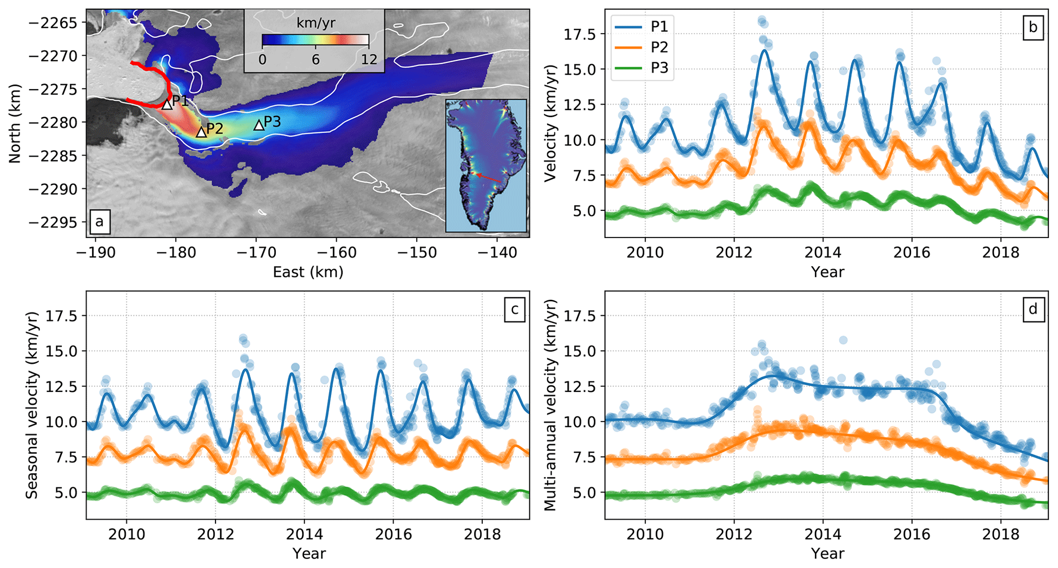
Figure 1Sermeq Kujalleq (Jakobshavn Isbræ) mean velocity field and select velocity time series. (a) Mean velocity between 2009 and 2019 in Polar Stereographic North (EPSG:3413) coordinates. The background image is a Landsat 8 image acquired in August 2017. White lines correspond to the bed topography (BedMachine V3) at sea level, and the red line indicates the winter 2017 terminus position (for all subsequent map figures). White triangles indicate the points P1–P3 from which data shown in (b–d) are taken. Inset shows (with red arrow) the approximate study area within Greenland with mean velocities from Joughin et al. (2011). (b) Time-dependent speed at points P1–P3. (c) Short-term velocity time series showing predominantly seasonal variations. For each time series, mean velocities for 2009–2019 have been added as offsets for visual clarity. (d) Long-term velocity time series showing the 2012 speedup and 2017 slowdown. In (b–d), solid lines show our model results while dots indicate (b) observed speeds or (c, d) detrended observations. The detrended short-term observations in (c) are the observed speeds minus the estimated integrated B-splines. The detrended long-term observations in (d) are the observed speeds minus the estimated seasonal B-splines.
4.1 Seasonal variations in surface velocity
The reconstructed velocity time series demonstrates the ability of our flexible method to smoothly interpolate the velocity data in time in a manner that preserves the seasonal variations. In particular, the use of temporally coherent B-splines to model seasonal variations allows for reconstruction of several summer speedup events where data happen to be more sparse for certain years (Fig. 1). By applying Eq. (5) to decompose the velocity magnitude time series into seasonal and transient components ( and , respectively), we show that short-term velocity variations on Jakobshavn Isbræ are dominated by the seasonal cycle of summer speedup and winter slowdown. In this section, we focus on these seasonal variations, leaving discussion of the multi-annual transient variations for the next section.
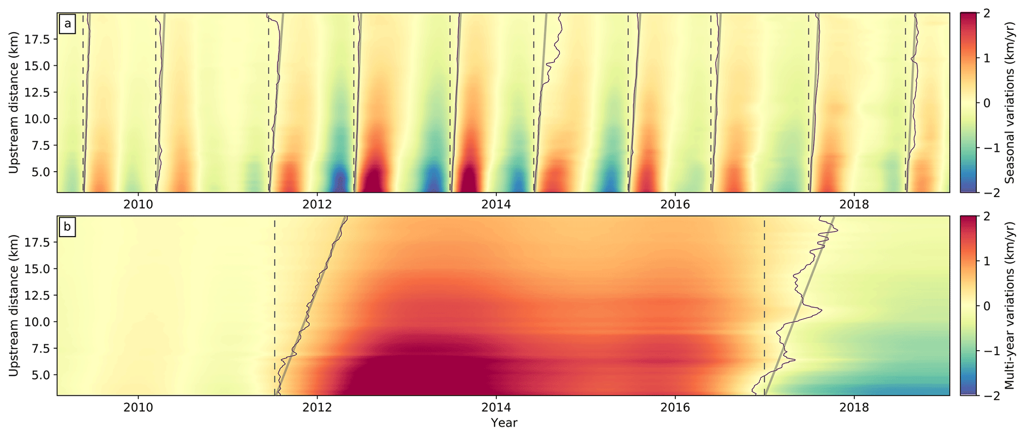
Figure 2Temporal evolution of glacier flow variations along a centerline segment for decomposed seasonal (a) and multi-year (b) signals. The centerline trace is shown in map view in Fig. 4, and distance values here are measured upstream along the centerline from the winter 2017 terminus position. Thin black lines correspond to contours of zero-velocity variation at the initiation of each signal – summer speedups for (a) and 2012 speedup and 2017 slowdown for (b). Solid gray lines approximately follow the zero-velocity contours and indicate the leading edges of propagating velocity variations. Vertical dashed gray lines indicate onset times for the propagating wave initiating at the terminus and are equivalent to the propagation path for a wave with infinite propagation speed. The tangent of the angle between solid and dashed gray lines is the phase velocity averaged over the observable propagation distance. The marked difference in phase velocities between the seasonal and multi-year signals indicates (frequency) dispersion.
The flexibility of the B-spline representation for the seasonal time series allows us to quantify the change in the amplitude of summer speedup from year to year and at each point on the glacier. In Figs. 1 and 2 we show these variations in two different views to aid in interpretation of the results. Figure 1a and b represent a classical view of spatiotemporal variations in surface velocity, with a map of secular velocity (Fig. 1a) and time series of select points on the glacier (Fig. 1b). Figure 1c shows, for the same points on the glacier, the seasonal variations, which are the total signal shown in Fig. 1b less the inferred multi-year trends discussed in the next section. In Fig. 2, we present a space–time plot for the (a) seasonal and (b) multi-year variations along the centerline transect shown in Fig. 4a. This representation allows for an intuitive visualization of spatiotemporal variations in the surface velocity fields and, most relevant for this study, the propagation of velocity variations through the glacier in time. Our analysis focuses on this propagation by treating velocity variations as traveling waves with quantifiable attenuation and propagation rates. To aid in this discussion, we have provided a visual representation of the upstream propagation rate in Fig. 2 using the solid and dashed black lines. The angle between the two lines represents the phase velocity cp, an important concept in this study that is defined as the speed at which the phase of a wave of a given frequency ω travels. Thus, , where kr is the real component of the angular wavenumber.
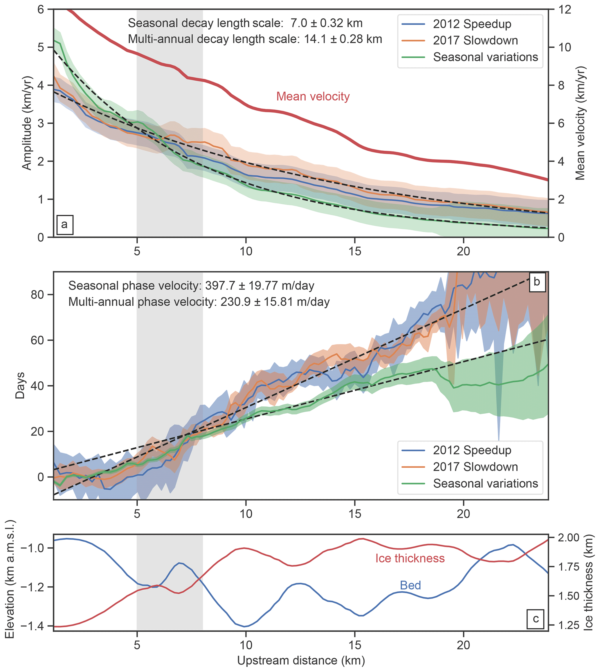
Figure 3Glacier centerline transects of phase delay and velocity variation amplitude for the seasonal, 2012 speedup, and 2017 slowdown signals compared to centerline ice thickness and bed depth. (a) Velocity variation amplitude and 1 SD (standard deviation) uncertainties for the three different signals. The decay length scale (e-folding distance) for the multi-annual signals is roughly twice that of the seasonal signal (represented by best-fit exponential decay model in dashed black lines). Dark-red line corresponds to the mean velocity magnitude along the centerline (note the 2× scaling factor for the mean velocity axis). (b) Relative phase delay for the three different signals: seasonal phase delay – green; 2012 speedup - blue; 2017 slowdown – orange. The upstream centerline distance is with respect to the intersection of the centerline and the 2017 terminus. For distances greater than 8 km upstream, the phase velocity for the seasonal signal is roughly twice as fast as the phase velocities for the multi-annual transients (represented by dashed black lines). The shaded areas represent the 1 SD formal uncertainties for the annual phase (green) and bootstrapped standard deviation for the transients (blue and orange). (c) Centerline ice thickness (red) and bed depth (blue) using bed data from BedMachine V3 (Morlighem et al., 2017). For all plots, the gray-shaded region represents the upstream region encompassed by the southern bend.
The results shown in Figs. 1c and 2a indicate that the amplitudes of seasonal velocity variations are largest near the terminus and decay as a function of upstream distance. By extracting a centerline transect of amplitude (averaged over all observed seasons) as a function of distance, we estimate an attenuation (or e-folding) length scale of approximately 7±0.3 km for all observed seasonal variations (Fig. 3a), which implies that large-amplitude velocity variations near the terminus position are observable at farther-upstream distances relative to smaller-amplitude variations. This effect can be observed by comparing in map view seasonal velocity variations for years when the amplitudes are markedly different (Fig. 4a and b). For the years 2009–2011 and 2017–2018, peak amplitudes of seasonal velocity variations did not exceed 3 km yr−1, whereas for the years 2012–2015 (the period with the fastest glacier flow speeds in our observations) the highest amplitudes exceed 6 km yr−1. Thus, there is a clear correlation between mean flow speed for a given year and the amplitude of seasonal variations, which we will explore in later sections.
In addition to attenuation, we are interested in constraining the rate of propagation of surface velocity variations. We quantify these variations in terms of phase velocities by constraining the relative timing of peak velocity for different temporal frequencies. As with amplitude, we present the absolute and relative timing of the velocity variations in multiple ways to help build a more intuitive framework for the reader. This presentation follows the same structure as the amplitude variations discussed in detail above, with a classical view shown in Fig. 1, the space–time diagram in Fig. 2, the mean over all seasons along a centerline transect in Fig. 3b, and a map view of the relative timing in Fig. 4c (with formal uncertainties in timing given in Fig. 4d).
For seasonal variations in surface velocity, the time of peak velocity varies slightly from year to year, with the earliest peaks occurring around mid-August and the latest peaks occurring around mid-September. The exception to this timing is the 2010 speedup which starts earlier in the year and may have been driven by a combination of warmer air temperatures and cooler ocean temperatures influencing mélange rigidity during the course of the seasonal cycle (Joughin et al., 2020a). Nevertheless, the spatial pattern of relative timing in the upstream direction from the terminus is broadly consistent even among years with large differences in mean velocities, which indicates a common mechanism for the seasonal cycle (Fig. 2a). As expected for marine-terminating glaciers like Jakobshavn Isbræ, the timing of the peak seasonal signal indicates that seasonal variations originate at the terminus and propagate upstream (Figs. 1c and 2a).
To investigate the spatial characteristics of the timing of peak velocity, we fit a simple temporal model using a sum of sinusoids to the velocity data from 2011 to 2019 at each pixel with the estimated long-term signals removed, dS (e.g., Fig. 1c), such that
where ωi is the angular frequency for the ith sinusoid; Ci and Si are the coefficients of the cosine and sine components, respectively; and C0 is a constant offset. After estimating the values of Ci and Si, the amplitude and phase (i.e., relative timing) of each sinusoid can be recovered as
While this model cannot accurately reproduce the amplitude changes or nonsinusoidal variations (e.g., Joughin et al., 2008, 2014), the seasonal phase can be estimated robustly with 7 years of data. Note that the years 2009–2010 are excluded in order to avoid introducing biases into the phase estimation from differences in onset times of summer speedups. Furthermore, we can compute the formal phase uncertainties following the procedure outlined in Minchew et al. (2017). The estimated seasonal phase is thus equivalent to the mean time of peak seasonal velocity for the 2011–2019 period while the phase uncertainty is proportional to the formal variance of the mean.
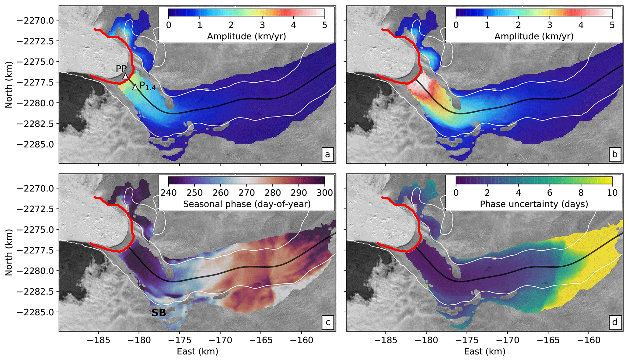
Figure 4Seasonal variations in flow speed and timing of peak velocities. (a) Mean seasonal velocity amplitude for the years 2009–2011 and 2017–2018 (years not associated with the increased velocities between 2012 and 2015). Triangular markers indicate comparison points used in Fig. 7: pinning point (PP) where the bed topography locally narrows and reference point 1.4 km upstream from the 2017 front position (P1.4). (b) Mean seasonal velocity magnitude variation for the years 2012–2015 (2016 excluded due to higher background velocities at the start of the summer). (c) Mean day of year of peak seasonal velocity (i.e., seasonal phase) for entire observation period. SB indicates the southern bend referred to in the text. (d) Seasonal phase uncertainty (1σ). Seasonal amplitudes are measured as the difference between the summer high and winter low velocities in the short-term time series as shown in Fig. 1c. The highest amplitudes occur at the terminus and decay exponentially upstream.
The seasonal phase map shows upstream transmission of velocity perturbations originating at the terminus (Figs. 3b and 4c). This propagation occurs rapidly in the first 5 km upstream of the terminus and then slows to a near-constant phase velocity of 398±20 m d−1 (approximately 146±7 km yr−1), which is more than an order of magnitude faster than the mean flow speed near the terminus. Our estimates of the phase velocity within the first 5 km upstream of the terminus are limited by the temporal resolution of the data, but by considering the uncertainties in timing, we estimate that the phase velocity in this region must be at least 500 m d−1 (182.5 km yr−1), or approximately 18 times the local mean glacier flow speed. In the across-flow direction, about 8 km upstream from the 2017 calving front, the center of the glacier reaches its peak velocity earlier than the margins by about 15 d, indicating a nonlinear relationship between time-dependent lateral shear strain rates and centerline velocity, meaning that the effective width of the shear margins (defined here as the centerline velocity divided by the maximum shear strain rate) must change over the seasonal cycle. Finally, we note that the phase uncertainty is generally lowest in the center of the glacier where amplitudes are higher and increases with distance upstream as the amplitudes decay (Fig. 4d), as expected from the formal uncertainties (Minchew et al., 2017).
4.2 Multi-year variations in surface velocity
After isolating the long-term signals from the short-term seasonal signals (i.e., ), we can observe clear variations in multi-annual amplitudes at different points along the glacier (Figs. 1d and 2b). The temporal density of the velocity time series allows us to quantify spatial variations in the amplitude and timing of the positive and negative multi-annual trends, much like we did with seasonal velocity variations in the previous sections. We observe two events in the data: a speedup that begins in 2012 and a slowdown that begins in late 2016 near the terminus, which we refer to as the 2017 slowdown. We present the results for multi-annual variations using the same general structure as for the seasonal ones, with the time series view shown in Fig. 1, the space–time diagram in Fig. 2, along a centerline transect in Fig. 3, and the map view of the amplitudes and phase values in Fig. 5.
The spatial pattern of the amplitudes of multi-annual velocity variations is remarkably consistent between the two observed events, with the highest amplitudes at the terminus and an exponential decay with distance upstream (Figs. 3a and 5a, b). Notably, the velocity variations induced by these events have an attenuation (e-folding) length scale of approximately 14.1±0.3 km, which is about twice the attenuation length for seasonal variations (Fig. 3a). As a result, we are able to observe multi-annual velocity variations farther upstream than the seasonal timescale velocity variations (Fig. 2b).
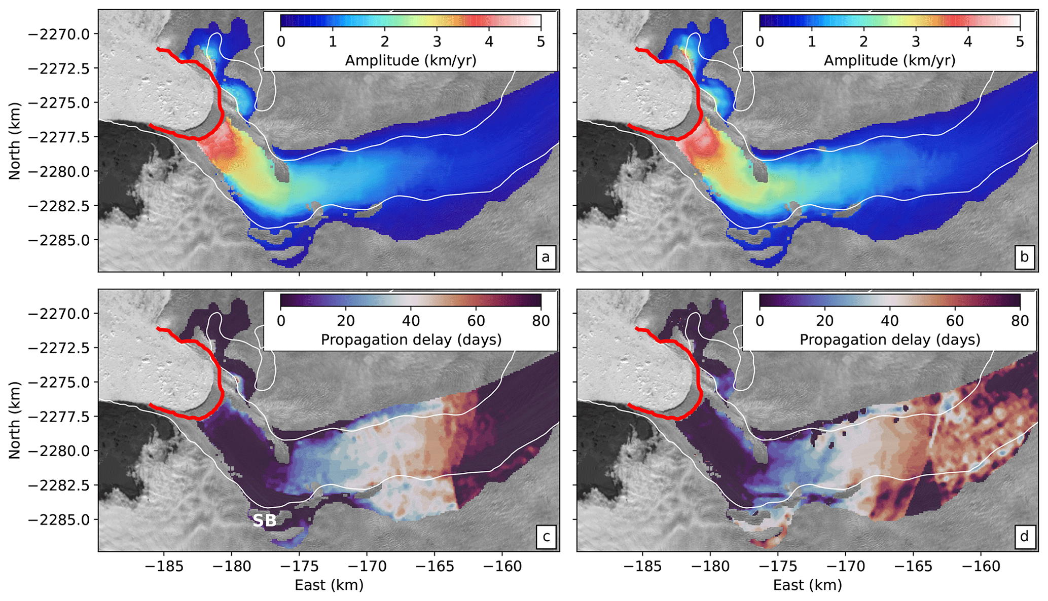
Figure 5Velocity variation amplitude and phase delay maps for 2012 transient speedup (a, c) and 2017 transient slowdown (b, d). In (c), SB indicates the southern bend referred to in the text. Red line indicates winter 2017 terminus position. In addition to the spatial distribution of phase delay and amplitude being consistent for the two events, these transient phase delays show strong similarities with the seasonal phase delay. However, the transient amplitudes show farther-upstream propagation than the seasonal amplitudes.
From the phase delay of the multi-annual signals, we can see that both the 2012 speedup and 2017 slowdown signals originate at the terminus, propagate rapidly along the first 5 km of the glacier, slow down through the southern bend between 5–8 km, and propagate upstream from 8–20 km at a generally consistent phase velocity (Figs. 3 and 5c, d). Beyond 20 km upstream, the amplitudes for the velocity variations become too low to reliably estimate the timing of arrival of the transient signals (Fig. 5d). The phase velocity between 8 and 20 km upstream is approximately 231±16 m d−1 (84±6 km yr−1), which is a little more than half of the phase velocity for the seasonal signal and roughly 7 times the mean flow speed near the terminus. For glaciers where ice flow is dominated by basal sliding, phase velocity is expected to scale with the square root of ice thickness and basal shear traction (Rosier et al., 2014), which is roughly consistent with the increase in phase velocity and ice thickness around 8 km upstream, although more work is needed to establish concrete connections. As with the observed seasonal variations, the phase velocity in the first 5 km upstream of the terminus is at the limit of the temporal resolution of the data with a lower bound on the phase velocity of at least 500 m d−1 (182.5 km yr−1), or approximately 18 times the mean glacier flow speed in this region. While the slowdown in wave propagation in the southern bend is coincident with a local high in the bed topography, more work is needed to evaluate whether the topographic effect is the dominant control on wave propagation. The apparent slowdown may also be an artifact of numerical errors caused by tracking of peak acceleration and deceleration rather than a multi-year average of the sinusoidal phase as for the seasonal signal. Nevertheless, the consistency in the spatial distribution of peak timing and amplitude reinforces the notion that a common physical mechanism is responsible for multi-year and seasonal velocity variations.
4.3 Multi-year variations in surface elevation
Ice surface elevation varies in response to changes in snow accumulation and melt (the sum of which constitutes the surface mass balance; SMB), firn compaction (Herron and Langway, 1980; Huss, 2013; Meyer et al., 2020), and dynamic thinning (thickening) in response to increases (decreases) in the flux divergence of the ice. The interplay between observed elevation and velocity changes at different temporal and spatial scales can thus yield insight into the mechanisms driving longer-term elevation and velocity changes.
For this work, the temporal sampling of the available elevation data (ArcticDEM and OMG DEMs) permits only the comparison of longer-term variations in velocity and elevation. Thus, we compare the long-term velocity and elevation changes for four successive time periods of length 2.2 years: (1) June 2010 to September 2012, (2) September 2012–November 2014, (3) November 2014–January 2017, and (4) January 2017 to March 2019 (Fig. 6).
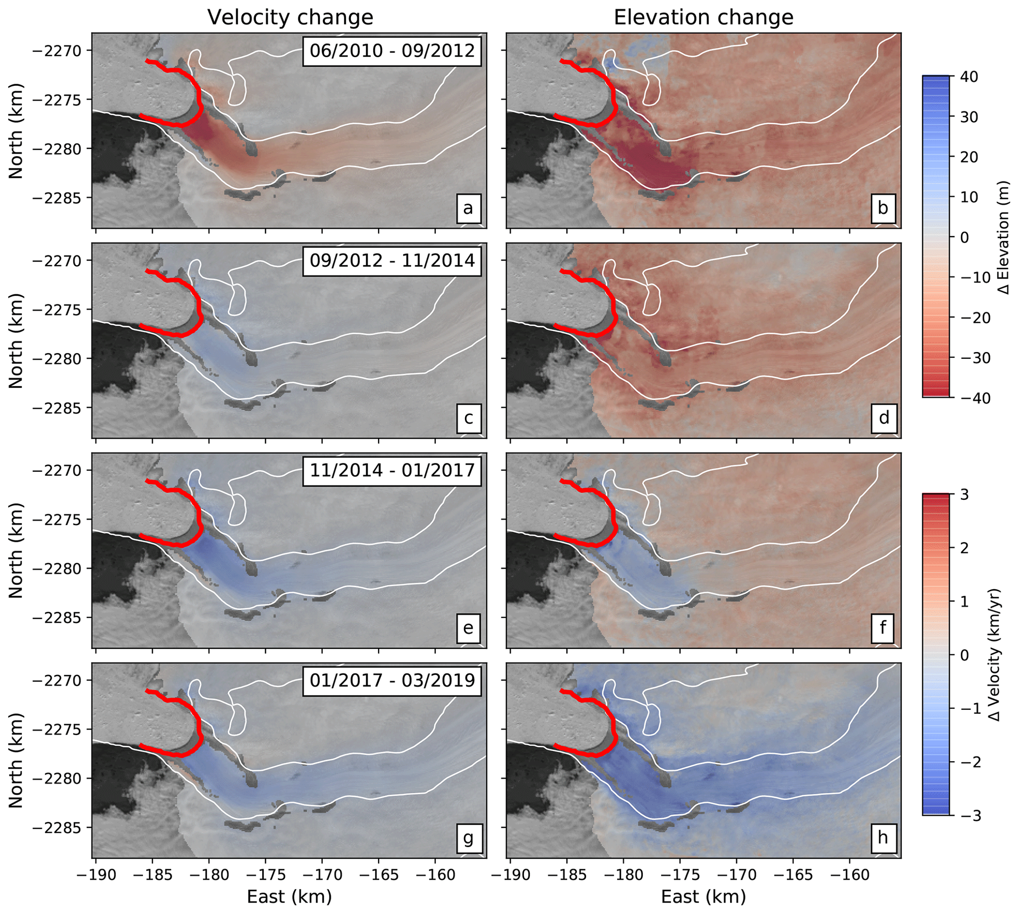
Figure 6Long-term velocity and ice surface elevation changes for successive time periods of 2.2 years. (a, b) June 2010 to September 2012: the glacier is accelerating (positive velocity anomaly) and thinning (negative elevation anomaly), with higher rates of thinning within the glacier. (c, d) September 2012 to November 2014: velocities show slight deceleration while the ice surface lowers over a wider area, indicating persistent surface melt. (e, f) November 2014 to January 2017: this time period contains the initiation of the 2017 slowdown, which is associated with ice thickening in the main trunk of the glacier. Note the continuing surface melt signal indicated by lowering distal to the glacier. (g, h) January 2017 to March 2019: slight decrease in glacier flow speed and more widespread increase in ice surface elevations due to positive SMB can be seen.
Within the main trunk of the glacier, we observe a clear association between the 2012 speedup and lowering of the ice surface due to dynamic thinning, whereas on the slower ice, thinning is more diffuse and occurs at a lower rate. A comparison of time series for points on and off the glacier (Fig. S1 in the Supplement) suggests that much of the ice in the surrounding areas has been lowering since before the observation period. In these areas, thinning has been attributed to inland diffusion of steepening surface slopes following speedup and thinning of the fast-flowing trunk in 2004 in response to disintegration of the ice tongue (Krabill et al., 2004; Joughin et al., 2008). The widespread lowering of the ice surface persists even during the slight deceleration of velocities over the glacier from 2012 to 2015 (Fig. 6c and d). During these years, the ice surface has likely adjusted to the initial speedup in 2012, leading to a reduction in driving stress and velocities. The 2017 slowdown is coincident with thickening of the ice on the main trunk of the glacier while the inland ice continues thinning (Joughin et al., 2018; Khazendar et al., 2019; Joughin et al., 2020a). From 2017 onwards, we observe more widespread thickening of the ice as the glacier velocities continued to decrease. Despite the recent thickening trend, elevation values are still measurably lower than they were in 2010, particularly for the ice outside of the main trunk of the glacier (Fig. S1).
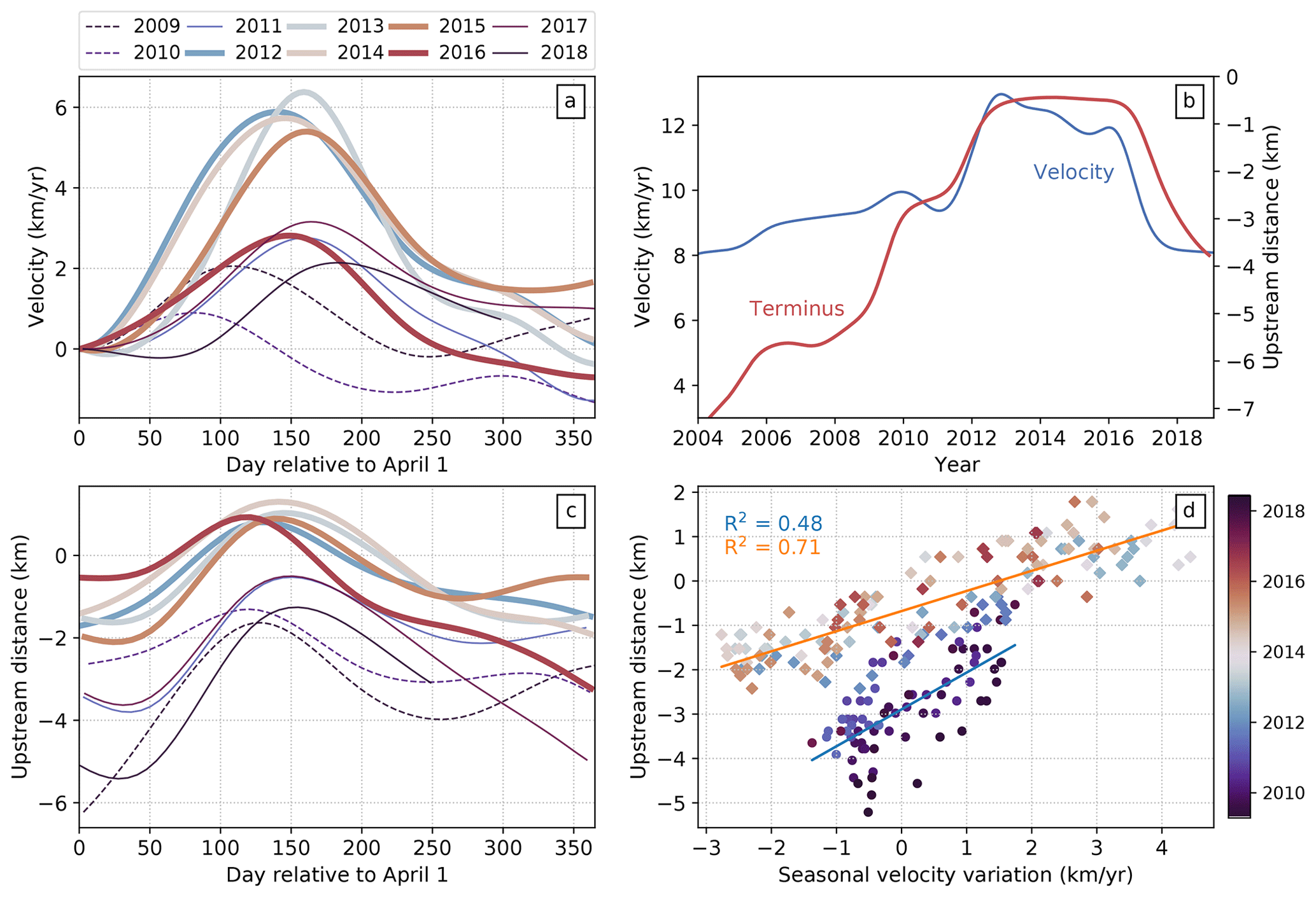
Figure 7Comparison between time series of observed terminus positions and ice velocities at various timescales. (a) Seasonal ice centerline velocity at a point 1.4 km upstream from the reference 2017 terminus position (location shown in Fig. 4). Speeds are shown on an annual timescale (referenced to 1 April) and are plotted relative to the speed on 1 April of the respective year. Line colors correspond to the color map in (d), and bold lines correspond to the years 2012–2016 where strong amplification of the seasonal variations is observed (Fig. 1). (b) Long-term ice velocity and terminus position. Velocities are extracted from the same point as in (a). Terminus positions are measured at the intersection of the time-varying calving front with the glacier centerline and are referenced to the position of the shallow pinning point highlighted by Cassotto et al. (2019). (c) Seasonal variations in terminus position with line colors and widths corresponding to lines in (a). (d) Correlation between terminus position and seasonal velocity (i.e., ) at the same location as in (a) and (b). Here, the points have been grouped into two temporal clusters: July 2011–January 2017 (diamonds) and all other times (circles), with the former time frame defined by the period when maximum seasonal retreat of the terminus position took it behind the reference pinning point. Thus, the scaling relationship between terminus position and velocities changes depending on whether the terminus has retreated beyond the pinning point. The text colors for the R2 values correspond to the trend-line colors, while the point colors in (d) correspond to line colors in (a) and (b).
4.4 Calving front forcing
The position of the calving front has been reported to be the dominant factor influencing ice dynamics for Jakobshavn Isbræ over observable, particularly seasonal, timescales (Nick et al., 2009; Joughin et al., 2012; Podrasky et al., 2012, 2014; Bondzio et al., 2017). The position of the calving front is heavily influenced by bed topography (Xu et al., 2013; Morlighem et al., 2016), local ocean temperatures that influence subaqueous melting of the terminus (Holland et al., 2008; Khazendar et al., 2019), and changes in mélange rigidity (Joughin et al., 2008; Cassotto et al., 2015; Robel, 2017; Xie et al., 2019; Joughin et al., 2020a). Changes in the calving front driven by iceberg calving can reduce back stresses upstream of the new calving front, allowing ice near the terminus to accelerate and subsequently thin. Local thinning of the ice steepens the surface slope, thereby increasing gravitational driving stress and causing further acceleration and thinning (Joughin et al., 2012). For glaciers where the calving front is located on a retrograde bed, the thinning-induced retreat of the terminus corresponds to increasing terminus ice thickness, which further increases the driving stress (Joughin et al., 2020a). The redistribution of mass during dynamic thinning propagates upstream as traveling waves, with phase velocities and attenuation length scales that we constrain using the methodology presented in this study. The thinning of the ice surface throughout the glacier is hypothesized to cause a further, indirect enhancement of velocities by causing a reduction in overburden pressure (weight of the ice column per unit area), which influences the response of the glacier to processes such as basal lubrication by drainage of surface meltwater in the summer melt season. While the role of basal lubrication has been shown to affect the seasonal cycle on certain glaciers (e.g., Howat et al., 2010; Bevan et al., 2015), the magnitude and timescale of the influence of basal lubrication on the velocities in Jakobshavn Isbræ remains unresolved.
Consistent with earlier work (e.g., Joughin et al., 2012; Cassotto et al., 2019) but using our method to decompose velocity time series into short- and long-term variations, we observe strong correlations between variations in ice velocity and variations in the front at both seasonal and long-term timescales (Fig. 7).
The timing of the maximum retreat for a given year is closely associated with the timing of peak seasonal ice velocity within a few kilometers of the front position. Here, we choose a point approximately 1.4 km upstream of the 2017 terminus in order to maximize data availability close to the front position for all years. For the 4 years associated with increased seasonal velocity amplitudes (2012–2015) during the summer, the calving front retreats past a narrow section in the bed referenced by Cassotto et al. (2019) (defined as our reference position for the terminus position time series and shown in Fig. S2) into the wider and deeper basin (values > 0 in Fig. 7c), which supports previous hypotheses that even subtle bed constrictions in the fjord can lead to large increases in ice velocity in response to terminus retreat when ice elevations are near flotation heights (Cassotto et al., 2019). In 2016, the calving front also retreats past the same pinning point, but the seasonal velocities do not reach the same peak as in the previous 4 years. In fact, in 2016, the calving front starts the summer melt season in a more retreated position, which is a consequence of the front not sufficiently advancing in 2015 and prematurely retreating in December of that year. Thus, while the seasonal amplitude in 2016 is less than in the previous 4 years, the absolute velocities are still high (Fig. 1c). For the years 2009–2011 and 2017–2018, the calving front does not retreat past the pinning point, which results in seasonal velocity variations with markedly smaller amplitudes.
Following Lemos et al. (2018), we compute the correlation between the measured calving front position (relative to the reference pinning point) and short-term velocities for the same point 1.4 km upstream of the 2017 terminus (Fig. 7d). The change in the velocity response to front variations between 2012 and 2015 can be clearly seen as a distinct cluster as compared to the other years in the observation period. For this 4-year period, a linear regression yields a coefficient of determination (R2) of 0.71 with seasonal velocities scaled by 2.2 km yr−1 per kilometer of front retreat. For the other years, the regression results in an R2 of 0.48 with a scale factor of 1.2 km yr−1 per kilometer of front retreat. Thus, from 2012 to 2015, the velocity response is more strongly correlated with front position with larger peak-to-peak variations than for the other years, presumably due to the retreat of the front past the reference pinning point described by Cassotto et al. (2019). The higher level of correlation for the years 2012–2015 is likely driven in part by the proximity of our point of comparison (1.4 km upstream of the 2017 terminus) to the retreated front position for those years. However, a comparison of the front position with velocities at a moving point 1 km upstream of the front still shows lower correlation for the years 2009–2010 (Joughin et al., 2020a), which underscores the importance of bed topography in the response of ice flow to front position.
On timescales longer than a year, calving front positions and multi-annual ice speeds also co-vary, but the relationship is more nonlinear than on seasonal timescales (Fig. 7b and d). After the disintegration of the ice tongue between 1998 and 2004 (Joughin et al., 2004), the front rapidly retreated about 4 km over the period from 2004 to 2011. During this time, the ice speed near the 2017 terminus increased by about 1.5 km yr−1, half of the roughly 3 km yr−1 increase associated with the 2012 speedup. The 2012 speedup on the other hand coincided with a 2 km retreat of the calving front (Fig. 7b).
Decomposition of the time-dependent velocity and surface elevation fields into distinct temporal scales reveals a repeating pattern on Jakobshavn Isbræ where velocity and surface elevation variations originate at the terminus. The coincidence of speedup and slowdown of the glacier with thinning and thickening, respectively, suggests a dynamic origin of the physical mechanism generating these variations. Prior studies have proposed that this mechanism is primarily characterized by a reduction in back stress at the terminus following a series of calving events, causing ice acceleration and increased driving stresses to propagate upstream which results in the observed high correlation between calving front position and velocity variations (e.g., Nick et al., 2009; Joughin et al., 2012; Bondzio et al., 2017). In this section, we detail the observed wave phenomena, introduce the proposition that the observed traveling waves are kinematic waves, and discuss possible paths for future development of observational methods that will enable progression toward robust and efficient techniques for fusing remote sensing data from multiple sources and using in situ observations as prior information to constrain the inversions.
5.1 Wave phenomena
Our results indicate that velocity variations initiating at the terminus of Jakobshavn Isbræ propagate upstream as traveling waves with frequency-dependent propagation speeds (phase velocities) and attenuation length scales. To our knowledge, ours are the first results to explicitly quantify wave propagation at seasonal and multi-annual timescales using remote sensing observations and, importantly, to show that traveling waves in this range of frequencies are dispersive, meaning that phase velocity is a function of frequency. These results on Jakobshavn Isbræ complement our inferences of wave propagation for hourly to fortnightly timescale variations in the flow speeds of Rutford Ice Stream, Antarctica, using remote sensing data (Minchew et al., 2017), helping to demonstrate the largely untapped potential of time-dependent remote sensing observations to quantify wave phenomena. Our ability to quantitatively observe wave propagation in glaciers using remotely sensed observations adds a new class of information and unique constraints to the mechanics of glacier flow – most notably the rheology of the ice–bed interface (i.e., the form of the sliding law) and the rheology of natural glacier ice – for the simple reason that these mechanics influence both the state of any given glacier and the transient response of the glacier to external forcing. At the moment, data sparsity only allows for quantification of phase velocities and attenuation length scales for describing overall wave propagation behavior. As more data become available, the time series methods outlined above should allow for observations of waveforms manifest in surface elevation fields in addition to constraints on dispersion relations (the relationship between frequency and wavelength) on individual glaciers that cover a broader range of frequencies with finer resolutions in the frequency domain. Realizing this potential for remote sensing time series is important because the characteristics of wave propagation, specifically the dispersion relation as defined for a wide range of frequencies, are intrinsic properties of dynamical systems if we define the system in this case such that it includes the glacier and boundary conditions. As such, time-dependent velocity and elevation data for glaciers characterized by a wide range of sliding speeds and geometries can be used to determine the relative contributions of forcing frequency, ice thickness, glacier width, and basal traction on measured phase velocities and attenuation length scales, thereby providing a method for inferring relevant mechanical and rheological parameters.
5.1.1 Observations of wave propagation
The most important and novel observables from this study are the phase velocities and attenuation length scales for seasonal and multi-annual velocity variations. Notably, both the phase velocities and attenuation length scales are frequency-dependent, with the higher-frequency seasonal signals propagating faster but not as far as the multi-annual signals. These results indicate that the traveling waves we observe, which appear to have a common source in the displacement of the calving front, are dispersive. This observation of dispersive wave propagation enables rich diagnostic tools to understand glacier mechanics, which we will explore in future work.
Physical insight can be gleaned from the absolute values of phase velocity (Fig. 3). One key takeaway from the absolute values are that the phase velocities we observe are everywhere at least an order of magnitude faster than the local mean (downstream) flow speeds of the glacier. We cannot estimate the fastest wave propagation speeds, which occur in the 5 km immediately upstream of the 2017 terminus position, because of the limited temporal resolution of the data. However, we estimate the lower bound on the phase velocity in this region based on the timing of the observations to be around 500 m d−1 (182.5 km yr−1), meaning that the traveling waves we observe propagate upstream at least 18 times faster than the local mean glacier flow speed. In the region 5–8 km upstream there is a reduction in phase velocities, and from 8–20 km upstream we find the slowest and best-constrained phase velocities at all frequencies. The propagation of these seasonal traveling waves is likely influenced by other indirect effects in the later part of the season, such as changes in overburden pressure due to ice thinning which can affect the response of ice flow to basal lubrication (Joughin et al., 2012).
The slowest phase velocities we report are for the multi-annual transient events that consist of a speedup centered in 2012 and a slowdown centered in 2017. Both the 2012 speedup and the 2017 slowdown have approximately the same phase velocity, which we find to be 231±16 m d−1 (84±6 km yr−1). Thus, whether associated with retreat (glacier speeds up) or advance (glacier slows down) of the terminus position, multi-annual signals propagate upstream roughly 7 times faster than the mean flow speed near the terminus of Jakobshavn Isbræ, or more than an order of magnitude faster than the local mean flow speeds. Taking both of the observed multi-annual signals to have periods of 3 years, we estimate the wavelength of the traveling waves to be km, where cp is the phase velocity and ω the angular frequency. At ∼50 times the width, ∼200 times the thickness of the glacier near the terminus, and ∼5 times the length of the glacier, the wavelength of observed multi-annual waves is much longer than any spatial dimension of the glacier. For seasonal frequencies, we observe phase velocities in the upstream 8–20 km section of 398±20 m d−1 (146±7 km yr−1), which is more than an order of magnitude faster than the glacier flow speed near the terminus. Taking the period of seasonal variations to be 1 year, we estimate the respective wavelength to be km. At ∼30 times the width and ∼100 times the thickness of the glacier near the terminus, the wavelength of seasonal variations is much longer than typical characteristic length scales for glacier flow but shorter than the multi-annual-period waves by a factor of approximately , as discussed below. The attenuation length scales we report for both seasonal and multi-annual-period traveling waves are more than an order of magnitude shorter than the wavelengths, consistent with previous studies of kinematic waves that found diffusive behavior with attenuation timescales shorter than their periods (Lick, 1970; Jóhannesson, 1992; Gudmundsson, 2003).
The wavelengths of the observed waves are perhaps clearer when considered in terms of the phase velocities. Using the same periods, we see that the ratio of phase velocities is approximately equal to the square root of the ratio of the frequencies, such that
in agreement with the estimates of wavelengths just discussed. This estimate places useful constraints on the form of the dispersion relation, which we will explore in future work. We note that the observed attenuation length scales appear to deviate somewhat from the square root–frequency relation as in Eq. (10), with the attenuation length scale for the seasonal signal being approximately half that for the multi-annual signal (Fig. 3). As with the phase velocities, this relationship between attenuation and frequency provides useful constraints on the dispersion relation.
Given the estimates of phase velocity at two different frequencies, it is desirable to estimate the group velocity, defined as the rate at which the envelope of a wave packet travels and thus the rate at which the energy of the wave packet travels. Mathematically, group velocity is defined as , where is the real component of the angular wavenumber. Our estimates of group velocity are crude given that we only observe waves with two frequencies and the period of the multi-annual signal is not well-defined because we use an integrated B-spline as a smooth step function to fit the transient. Nonetheless, assuming, as before, that seasonal signals have a period of 1 year and the observed multi-annual signals both have periods of 3 years, we estimate a group velocity of cg≈230 km yr−1, which is faster than the respective phase velocities. Therefore, in this relation between phase and group velocities, the waves we observe are analogous to capillary waves, though the analogy goes no further as the physical mechanisms governing capillary waves are not all applicable to the low-Reynolds-number regime of glacier flow.
The wave speeds we observe on Jakobshavn Isbræ are appreciably faster than those observed on Mer de Glace, France, even when we correct for the differences in mean flow speed between the two glaciers. Traveling wave speeds on Mer de Glace following numerous perturbations in surface mass balance were synthesized by Lliboutry and Reynaud (1981) to be in the range of 450–725 m yr−1, or about 4–6 times the mean flow speed of the glacier. The traveling waves we observe on Jakobshavn Isbræ are moving 2 orders of magnitude faster upstream than traveling waves on Mer de Glace. The ratio of phase velocity to local mean flow speed is roughly a factor of 2 higher on Jakobshavn Isbræ than Mer de Glace. There are marked differences in these two glaciers and the proposed perturbing forces are quite different – retreat of the terminus on Jakobshavn Isbræ and perturbation in surface mass balance on Mer de Glace – but the qualitative differences in observed wave propagation speeds are noteworthy.
When comparing the results presented here with observed wave propagation on other glaciers, we note dramatic differences between the phase velocities and attenuation length scales on Jakobshavn Isbræ and wave propagation related to much higher-frequency (14.76 d period) variations in ice surface velocity that we previously reported for Rutford Ice Stream, West Antarctica (Minchew et al., 2017). On Rutford Ice Stream – with a mean flow speed near the grounding line of approximately 375 m yr−1 – velocity variations driven by ocean tides propagate upstream with a phase velocity of approximately 24 km d−1 for the first 40 km upstream of the grounding line and then at a faster rate of 34.3 km d−1 further upstream. Thus, observed waves on Rutford Ice Stream propagate 2 orders of magnitude faster than those we observe on Jakobshavn Isbræ. The attenuation length scales are also markedly different: approximately 45 km on Rutford Ice Stream versus 7 km (seasonal) and 14 km (multi-annual) on Jakobshavn Isbræ. Several observational and modeling studies have suggested that at Rutford Ice Stream, downstream variations in buttressing stresses over the ice shelf, grounding line position, and/or water pressure at the bed (Gudmundsson, 2006, 2007; Rosier et al., 2014, 2015; Minchew et al., 2017; Robel et al., 2017; Rosier and Gudmundsson, 2020) drive the variations in flow speed over the tidal cycle. The marked differences in forcing frequencies and propagation speeds and distances between Rutford Ice Stream and Jakobshavn Isbræ therefore suggest fundamental differences in wave types and forcing mechanisms. Indeed, while previous work cited above suggests that waves on Rutford Ice Stream are influenced by the viscoelastic properties of ice expected at fortnightly periods, the much longer periods of variability on Jakobshavn Isbræ render elasticity of glacier ice negligible and thus unlikely to contribute in any meaningful way to wave propagation. We further discuss the distinctions between wave types below.
5.1.2 Kinematic wave propagation
We hypothesize that the traveling waves we observe can be classified as kinematic waves because of their long periods (months to years), their strong correlation with the calving front position, and marked dynamical thinning of the glacier corresponding to increases in velocity. Kinematic waves represent a special case in a broader spectrum of wave behavior that includes various forms of dynamical waves. As the name suggests, dynamical waves are driven primarily by pressure and stress gradients and arise in a variety of contexts, such as seismic waves, flexural waves (Lipovsky, 2018), shallow-water waves, so-called “seasonal waves” on glaciers (Fowler, 1982; Hewitt and Fowler, 2008), and the response of outlet glaciers to ocean tides (Rosier et al., 2015; Rosier and Gudmundsson, 2016; Minchew et al., 2017). On the other hand, kinematic waves arise primarily from the redistribution of mass, with propagation characteristics dominated by mass conservation rather than momentum balance. Kinematic waves have been used to model phenomena as varied as glacier surges, river floods, and traffic flow (Lighthill and Whitham, 1955; Nye, 1958, 1960). All waves on glaciers will be driven by some combination of dynamic (momentum balance) and kinematic (mass balance) processes, and the dominance of one driving mechanism over another informs the broad characteristics of the full dispersion relation for any given glacier at any given time.
Our hypothesis that the waves we observe are kinematic waves is consistent with previous studies that explore various aspects of kinematic wave propagation and the response of tidewater glaciers to changes in terminus position, from observations (Howat et al., 2005; Joughin et al., 2008; Felikson et al., 2017) to flow models (Thomas, 2004; Pfeffer, 2007; Nick et al., 2009; Joughin et al., 2012; Williams et al., 2012). Often, these arguments are based on the logical conclusion of progressive drawdown of the glacier surface. In essence, this process plays out such that changes in the terminus position through calving locally alter longitudinal (normal) stresses, allowing the glacier to locally accelerate. The local acceleration alters longitudinal stresses and increases flux divergence, causing the glacier to thin. Localized thinning steepens the surface slope, thereby increasing gravitational driving stress and generating upstream acceleration (Joughin et al., 2012). The process repeats as the surface is progressively drawn down, and a wave propagates upstream. Similar mechanisms operate in reverse for re-advance of the terminus position. This explanation is broadly consistent with our observations showing that changes in surface elevation are coincident with changes in surface velocity (Fig. 6). We reserve for future work a detailed exploration of wave propagation in glaciers, including tests of the kinematic-wave explanation of the observations we present in this study.
However, we note two important caveats to the applicability of the kinematic-wave description to our observations. The first is that the wave speeds we observe are an order of magnitude faster than the local mean flow speeds, making them much faster than kinematic-wave speeds proposed previously (Nye, 1960; Lliboutry and Reynaud, 1981; Weertman and Birchfield, 1983; van de Wal and Oerlemans, 1995). This discrepancy likely arises from a combination of the assumptions made in previous estimates and the fact that our observed phase velocities are not corrected for diffusivity and so are not direct measurements of the kinematic-wave speed (Lliboutry and Reynaud, 1981). As an example of the assumptions made in earlier estimates of kinematic-wave speeds, Nye (1960) assumed a shallow-ice approximation for the flow regime (wherein gravitational driving stress is balanced locally at the bed) and a power–law relation between the slip rate and drag at the ice–bed interface (i.e., the sliding law) with values for the exponent defined by Weertman (1957) for regelation and viscous flow of ice around roughness features in a monochromatic bed. Such a sliding law does not account for the full range of possible sliding mechanisms (Schoof, 2005; Joughin et al., 2019; Zoet and Iverson, 2020; Minchew and Joughin, 2020), meaning that estimates from Nye (1960) and others that follow the same basic formulation do not capture the range of possible values for kinematic-wave speeds. More work is needed to reconcile our observations with models of traveling wave propagation.
The second caveat to our conclusion that the waves we observe are kinematic waves is that our observations indicate that the observed waves are dispersive. Recall that we define dispersion in the traditional sense to mean “frequency dispersion” – the frequency dependence of wave speed – whereas some authors, notably Lighthill and Whitham (1955), use the term “amplitude dispersion” to describe the amplitude dependence of wave speed. The latter is a general characteristic of kinematic waves that can cause waveforms to change shape as faster waves overtake slower waves (Fowler, 1982, 2011). However, the amplitude dependence of wave speed does not account for our observations for three reasons. First, the phase velocity of waves with seasonal periods are relatively consistent despite large differences in the amplitude of seasonal variations (Fig. 2). Second, the multi-annual variations in glacier flow speeds have comparable amplitudes to the seasonal variations and yet propagate more slowly by a factor of , nearly equal to the square root of the ratio of frequencies (Eq. (10) and Fig. 3). Third, the observed phase velocities for the 2012 speedup and 2017 slowdown propagate at nearly the same speed (Fig. 3) despite different amplitudes of variations in surface flow speed (Figs. 1 and 2) and elevation (Fig. 6). Thus, we conclude that differences in amplitude cannot explain the disparities in phase velocities from waves with seasonal and multi-annual periods. Our observations, therefore, provide evidence of (frequency) dispersion in traveling waves.
Evidence for dispersion is noteworthy in part because kinematic waves on glaciers are governed by the continuity equation, which can be expressed in the form of the first-order wave equation; kinematic waves are, therefore, non-dispersive in the classical theory (Lighthill and Whitham, 1955; Nye, 1960). More recent work by, for example, Pfeffer (2007) and Felikson et al. (2017) presents models for tidewater glaciers that are similar to the classical kinematic-wave models and are likewise non-dispersive. While we leave for future work a detailed theoretical model accounting for dispersion in waves with seasonal to multi-annual periods, we speculate on a few possible sources of dispersion. The first candidate for the source of dispersion can be broadly defined as effects from longitudinal (extensional) normal stresses on wave propagation. If important, longitudinal stresses would entail inclusion of dynamical processes operating with greater importance than or equal importance to the kinematic-wave processes. As mentioned previously, kinematic waves are special cases in a broader spectrum of wave phenomena that must include various types of dynamical waves, and we should expect there to be a range of frequencies in which both mass and momentum balances play non-negligible roles in wave propagation.
The rheology of ice is another candidate for dispersion. We may intuitively expect waves with periods comparable to the viscoelastic relaxation time (ratio of dynamic viscosity to shear modulus) to be dispersive as the combination of viscous and elastic responses mean that waves of different frequencies will travel through ice with different effective rheologies. In this case, the restoring force provided by elasticity is proportional to strain, which will vary with wavelength. However, the periods of waves we observe are much longer than the viscoelastic relaxation time – which is typically on the order of hours to weeks (Gudmundsson, 2007) – meaning that ice is essentially a purely viscous fluid over the timescales relevant for our observations, and therefore elasticity is an unlikely source of dispersion. The non-Newtonian viscosity of ice is also unlikely to generate dispersion in kinematic waves due to the long periods of the wave relative to the viscoelastic relaxation time, which is supported by previous studies of kinematic waves (Nye, 1960; van der Veen, 2001; Pfeffer, 2007; Felikson et al., 2017).
Other obvious physical processes that could give rise to dispersion in traveling waves with seasonal and multi-annual periods are related to water pressure at the bed. In the interest of brevity, we divide the relevant processes into two broad categories: subglacial hydrology and till porosity. For subglacial hydrology, the well-known dependence of the hydrological pressure gradient on the surface slope of the glacier may be an important consideration (Flowers, 2015). After all, kinematic waves propagate upstream due to a progressive drawdown of the surface, which entails a transient steepening of the surface slope. The response of the subglacial hydrological system to the transient changes in glacier geometry are beyond the scope of this study and are worthy of further consideration in future work. As another example, dilation and compaction of subglacial till has recently received attention as a possible mechanism for triggering surges in glaciers with deformable beds (Minchew and Meyer, 2020) and has long been considered a potentially important mechanism in the centennial-timescale dynamics of ice streams (Tulaczyk et al., 2000; Robel et al., 2016; Meyer et al., 2019). In this mechanism, till dilation is influenced by the overburden pressure at the bed (i.e., the weight of ice per unit area) and the change in slip rate at the bed. As the surface velocity increases, it is likely that a corresponding increase in slip rate manifests at the bed and can be expected to cause the deforming till layer to dilate. For realistic values of hydraulic permeability of the till, dilation will cause a temporary decrease in pore water pressure. Minchew and Meyer (2020) showed that this processes can (in an idealized model) lead to glacier surges by delaying the evolution of the till to a new steady state. In a related sense, dilation and the subsequent evolution of pore water pressure provide a possible mechanism for altering the mechanical properties of the glacier bed in such a way that might generate dispersion in waves with seasonal and multi-annual periods.
5.2 Applicability to other study areas
The GIMP velocity data over Jakobshavn Isbræ exhibit strong, well-defined, short- and long-term variations, which facilitates reconstruction of the spatiotemporal evolution of the traveling waves discussed in this work. Additionally, the dense temporal sampling relative to the signals of interest avoids potential issues related to oversmoothing of short-term velocity variations. However, many other glaciers and ice streams in Greenland and Antarctica will not have the same level of data coverage as Jakobshavn Isbræ, which may limit the recovery of similar dynamical signals. Data coverage in this context is specified by temporal sampling and spatial continuity of velocity data where the former is likely to be the primary limiting factor for time series analysis. For example, velocity data derived primarily from optical platforms are generally restricted to the summer months where cloud and snow cover effects are minimized. This asymmetry in coverage for a given year will alias reconstruction of seasonal velocity cycles, which would likely cause artifacts when attempting to quantify wave properties like phase velocity. We estimate that velocity data provided at monthly intervals constitute the lower bound for the temporal resolution in order to quantify wave behavior at sub-annual timescales using the methods presented here. Of course, higher phase velocities for certain classes of dynamical signals may necessitate remote sensing data with a finer temporal resolution (Minchew et al., 2017).
Spatial resolution and spatial data gaps can also limit characterization of wave behavior and other changes in ice flow. For example, regions near glacier termini will undergo periods of missing data associated with termini retreat where velocity data cannot be obtained over open water. The temporal interpolation properties of B-splines can mitigate these effects to some degree, but study areas with more persistent spatial gaps will likely benefit from incorporation of spatial coherency, which enforces that neighboring grid points share similar temporal behavior. However, data that require stronger levels of spatial coherency may also result in reconstructed signals that are oversmoothed, which would bias phase velocities and decay length scales to lower and higher values, respectively. In these situations, it would be beneficial to incorporate independent data sources like GPS time series to provide additional validation data for “tuning” the time series analysis parameters. Overall, we expect that current and future remote sensing platforms will provide high-quality data similar to the GIMP data over Jakobshavn Isbræ, and we discuss those implications next.
5.3 Future work in remote sensing
The increasing availability of surface velocity and elevation fields sampled at monthly to sub-monthly timescales will continue to provide opportunities to study the rapid evolution of fast-flowing glaciers to various environmental forcings. The operational capabilities of several working groups that produce velocity fields over the Greenland and Antarctic ice sheets will consistently improve as new data are made available and techniques for generating velocity estimates are refined. In particular, the upcoming NASA-ISRO Synthetic Aperture Radar (NISAR) mission will generate unprecedented volumes of data that are useful for quantifying surface change for a number of scientific applications, including glacier dynamics (Aeronautics and Administration, 2018). The wide imaging swath (∼240 km) coupled with a 12 d repeat cycle and global coverage will allow for systematic observations of high-resolution velocity variations over interconnected glacier networks and coupled ice stream and ice shelf systems. Such observations will facilitate quantification of the spatiotemporal responses of glaciers and ice streams to any changes to the stress state, such as changes to the terminus position, loss of ice shelf buttressing, changes in frictional properties of the bed, and evolution of the subglacial hydrology. These processes will likely result in wave phenomena similar to those observed at Jakobshavn Isbræ (this study) and Rutford Ice Stream (Minchew et al., 2017) and would be well-observed with platforms like NISAR. Furthermore, the quantification of phase velocities and attenuation length scales at multiple forcing frequencies would provide valuable constraints on a general theory for wave propagation for fast-flowing glaciers because the characteristics of wave propagation are intrinsic properties of any given glacier system, which includes the boundary conditions.
The temporal resolution of surface DEMs is currently a limiting factor in quantifying sub-annual dynamical thinning. In this study, we noted that the thinning signal in the ice adjacent to the fast-flowing regions may be due to oversmoothing of the time series due to the limited temporal resolution of the ArcticDEM dataset. Therefore, elevation or altimetry datasets that have increased temporal sampling, such as ICESat-2, may help isolate the shorter-term dynamic signals from any longer-term SMB-based variations. In particular, future analysis would benefit from the 91 d repeat time of ICESat-2 for capturing seasonal elevation variations for direct comparison and synthesis with the velocity seasonal variations. This type of analysis could lead to a full three-dimensional velocity time series, which has the potential to improve quantification of strain and stress fields, constraints on ice rheology, and assimilation of velocity data into state-of-the-art ice flow models. For glaciers and ice streams where a persistent ice shelf or tongue exists, tidal forcing may become an important stress perturbation, in which case accurate reconstruction of vertical displacements would be necessary in order to constrain the dominant tidal constituents of motion (Minchew et al., 2017).
The flexible time series framework described here introduces the potential for using in situ observations as prior information (encoded in the prior model covariance matrix Cm) in forming time-dependent surface velocity fields. One example of this synergy between remote sensing and in situ data is the use of GPS and GNSS observations to constrain the form of the temporal basis functions, as we did in Minchew et al. (2017). A similar constraint may be obtained from terrestrial radar instruments that record velocity variations at timescales of minutes, allowing for high-resolution observations of dynamic responses to calving events or mélange collapse (e.g., Xie et al., 2019; Cassotto et al., 2019). In those situations, temporal basis functions and spatial correlations between basis functions can be used for dictionary construction and time series inversions. Another, less obvious, example is the potential for employing catalogs of calving events gleaned from seismic observations (Olsen and Nettles, 2017, 2019; Olinger et al., 2019) to constrain the timing and duration of transient accelerations in ice flow. Such constraints on the temporal evolution of the fields observed from remote sensing observations should afford novel opportunities to constrain phenomena such as the localization of strain rates (and, thereby, stresses) associated with fracture and calving. We expect the usefulness of the flexible methods we present here to grow as more remote sensing and in situ data become available.
We have presented a framework for forming continuous time-dependent surface velocity and elevation fields from publicly available surface velocity and elevation data. This framework is based on a sparsity-regularized linear-regression method that reconstructs time series as a linear combination of relevant basis functions. The flexibility and expressive power of the basis function representation allows for accurate reconstruction of time series in the presence of noisy and missing data while also allowing for a natural decomposition of the total signal into signals of multiple temporal scales. Over Jakobshavn Isbræ, this decomposition permitted a detailed investigation into the spatiotemporal characteristics of the evolving seasonal cycle of ice speedup and slowdown which are shown to be highly correlated to seasonal terminus variations. Analogously, longer-term changes in velocity were isolated and also highly correlated with longer-term terminus variations. This type of analysis is directly applicable to many outlet glaciers in Greenland, Antarctica, and other areas where multitemporal remote sensing data are available and could improve our understanding of the dynamic response of glaciers to various geographic and environmental forcings.
We demonstrated that the time series reconstruction permitted the quantification of traveling wave propagation resulting from terminus forcing functions at different temporal frequencies. These results build upon an important new area of research that aims to achieve a mechanistic understanding of glacier flow from time-dependent velocity data. To our knowledge, our results are the first to show from observations that waves on glaciers with seasonal to multi-annual periods are dispersive, with a ratio of observed phase velocities approximately equal to the square root of the ratio of frequencies. We hypothesize that the observed waves can be classified as kinematic waves based on their long periods (much longer than the viscoelastic relaxation time), their correlation with changes in the terminus position, and coincident variations in surface velocity and elevation. However, the dispersive nature and higher phase velocities of the observed waves relative to previously proposed kinematic waves necessitate further investigation into their physical drivers and the overall dynamic response of glaciers to stress and mass perturbations. These observations of traveling waves are only possible due to the strong velocity response to changes in terminus position, as well as due to our ability to isolate short- and long-term signals in the velocity data. Looking forward, we aim to assimilate other velocity sources for Jakobshavn Isbræ (e.g., optical or Sentinel-1), as well as other elevation and altimetry datasets, to improve temporal sampling and to obtain full 3D surface velocity time series. The resultant dataset will likely lead to a marked improvement in incorporating velocity data into ice flow models for simulation and inversion of mechanical properties.
The time series analysis and decomposition tools are available at https://doi.org/10.5281/zenodo.4474829 (Riel, 2021).
The velocity data are available at NSIDC (NSIDC-0481 at https://doi.org/10.5067/YXMJRME5OUNC) (Joughin et al., 2020b). The original ArcticDEM elevation data are available from the Polar Geospatial Center, University of Minnesota (ArcticDEM at https://doi.org/10.7910/DVN/OHHUKH) (Porter et al., 2018) while the OMG DEM data are available at https://doi.org/10.5067/OMGEV-GLNA1 (last access: October 2019) (Fenty et al., 2016). The pre-2017 calving fronts obtained in this study are available from https://doi.org/10.1594/PANGAEA.897066 (Zhang et al., 2019). The post-2017 calving fronts delineated from TerraSAR-X data are available at the University of Washington ResearchWorks Archive at https://doi.org/10.6069/XQS7-CD47 (Joughin et al., 2020a). Landsat 8 imagery is available from EarthExplorer (https://earthexplorer.usgs.gov, last access: June 2020) (USGS, 2020). The bed elevation (BedMachine v3) is available at NSIDC (https://nsidc.org/data/IDBMG4, last access: September 2019) (Morlighem et al., 2017).
The supplement related to this article is available online at: https://doi.org/10.5194/tc-15-407-2021-supplement.
BR and BM conceived the project, analyzed the data, and wrote the manuscript. IJ processed the GIMP data and provided valuable insights and feedback on the manuscript.
The authors declare that they have no conflict of interest.
The authors thank the two anonymous reviewers for their constructive feedback for improving the quality of this work. The authors also thank Jerome Neufeld, Ian Hewitt, Denis Felikson, and Colin Meyer for insightful discussions.
This research has been supported by the National Science Foundation (grant no. OPP-1739031).
This paper was edited by Andreas Vieli and reviewed by two anonymous referees.
Aeronautics and Administration: NASA-ISRO SAR (NISAR) Mission Science Users' Handbook, Jet Propulsion Laboratory, National Aerounatics and Space Administration, available at: https://nisar.jpl.nasa.gov/system/documents/files/26_NISAR_FINAL_9-6-19.pdf (last access: September 2019), 2018. a
Bevan, S. L., Luckman, A., Khan, S. A., and Murray, T.: Seasonal dynamic thinning at Helheim Glacier, Earth Planet. Sc. Lett., 415, 47–53, https://doi.org/10.1016/j.epsl.2015.01.031, 2015. a
Bishop, C. M.: Pattern recognition and machine learning, Springer, New York, USA, 2006. a, b
Bondzio, J. H., Morlighem, M., Seroussi, H., Kleiner, T., Rückamp, M., Mouginot, J., Moon, T., Larour, E. Y., and Humbert, A.: The mechanisms behind Jakobshavn Isbræ's acceleration and mass loss: A 3-D thermomechanical model study, Geophys. Res. Lett., 44, 6252–6260, https://doi.org/10.1002/2017GL073309, 2017. a, b, c
Cassotto, R., Fahnestock, M., Amundson, J. M., Truffer, M., and Joughin, I.: Seasonal and interannual variations in ice melange and its impact on terminus stability, Jakobshavn Isbræ, Greenland, J. Glaciol., 61, 76–88, https://doi.org/10.3189/2015JoG13J235, 2015. a
Cassotto, R., Fahnestock, M., Amundson, J. M., Truffer, M., Boettcher, M. S., De La Peña, S., and Howat, I.: Non-linear glacier response to calving events, Jakobshavn Isbræ, Greenland, J. Glaciol., 65, 39–54, https://doi.org/10.1017/jog.2018.90, 2019. a, b, c, d, e, f, g
Dehecq, A., Gourmelen, N., and Trouvé, E.: Deriving large-scale glacier velocities from a complete satellite archive: Application to the Pamir–Karakoram–Himalaya, Remote Sens. Environ., 162, 55–66, https://doi.org/10.1016/j.rse.2015.01.031, 2015. a
ESA: Greenland Ice Sheet CCI Calving Front Location, available at: http://esa-icesheets-greenland-cci.org/index.php?q=CFL (last access: 21 August 2019), 2016. a
Fahnestock, M., Scambos, T., Moon, T., Gardner, A., Haran, T., and Klinger, M.: Rapid large-area mapping of ice flow using Landsat 8, Remote Sens. Environ., 185, 84–94, https://doi.org/10.1016/j.rse.2015.11.023, 2016. a
Felikson, D., Bartholomaus, T. C., Catania, G. A., Korsgaard, N. J., Kjær, K. H., Morlighem, M., Noël, B., Van Den Broeke, M., Stearns, L. A., Shroyer, E. L., Sutherland, D. A., and Nash, J. D.: Inland thinning on the Greenland ice sheet controlled by outlet glacier geometry, Nat. Geosci., 10, 366–369, https://doi.org/10.1038/ngeo2934, 2017. a, b, c, d
Fenty, I., Willis, J. K., Khazendar, A., Dinardo, S., Forsberg, R., Fukumori, I., Holland, D., Jakobsson, M., Moller, D., Morison, J., Meunchow, A., Rignot, E., Schodlock, M., Thompson, A. F., Tino, K., Rutherford, M., and Trenholm, N.: Oceans Melting Greenland: Early results from NASA's ocean-ice mission in Greenland, Oceanography, 29, 72–83, https://doi.org/10.5670/ocean.2016.100, 2016. a
Flowers, G. E.: Modelling water flow under glaciers and ice sheets, P. Roy. Soc. A, 471, 20140907, https://doi.org/10.1098/rspa.2014.0907, 2015. a
Fowler, A.: Mathematical geoscience, in: vol. 36 of Interdisciplinary Applied Mathematics, Springer-Verlag, London, https://doi.org/10.1007/978-0-85729-721-1, 2011. a, b
Fowler, A. C.: Waves on glaciers, J. Fluid Mech., 120, 283–321, https://doi.org/10.1017/S0022112082002778, 1982. a, b
Gardner, A., Fahnestock, M., and Scambos, T.: ITS_LIVE Regional Glacier and Ice Sheet Surface Velocities, NSIDC – National Snow and Ice Data Center, University of Colorado, Boulder, Colorado, USA, https://doi.org/10.5067/6II6VW8LLWJ7, 2019. a
Gardner, A. S., Moholdt, G., Scambos, T., Fahnstock, M., Ligtenberg, S., van den Broeke, M., and Nilsson, J.: Increased West Antarctic and unchanged East Antarctic ice discharge over the last 7 years, The Cryosphere, 12, 521–547, https://doi.org/10.5194/tc-12-521-2018, 2018. a, b
Goldstein, R. M., Engelhardt, H., Kamb, B., and Frolich, R. M.: Satellite radar interferometry for monitoring ice sheet motion: Application to an Antarctic Ice Stream, Science, 262, 1525–1530, https://doi.org/10.1126/science.262.5139.1525, 1993. a
Gudmundsson, G. H.: Transmission of basal variability to a glacier surface, J. Geophys. Res., 108, 1–19, https://doi.org/10.1029/2002JB002107, 2003. a
Gudmundsson, G. H.: Fortnightly variations in the flow velocity of Rutford Ice Stream, West Antarctica, Nature, 444, 1063–1064 https://doi.org/10.1038/nature05430, 2006. a
Gudmundsson, G. H.: Tides and the flow of Rutford Ice Stream, West Antarctica, J. Geophys. Res.-Earth, 112, F04007, https://doi.org/10.1029/2006JF000731, 2007. a, b
Herron, M. M. and Langway, C. C.: Firn Densification: An Empirical Model, J. Glaciol., 25, 373–385, https://doi.org/10.3189/S0022143000015239, 1980. a
Hetland, E., Musé, P., Simons, M., Lin, Y., Agram, P., and DiCaprio, C.: Multiscale InSAR time series (MInTS) analysis of surface deformation, J. Geophys. Res.-Solid, 117, B02404, https://doi.org/10.1029/2011JB008731, 2012. a, b, c
Hewitt, I. J. and Fowler, A. C.: Seasonal waves on glaciers, Hydrol. Process., 22, 3919–3930, https://doi.org/10.1002/hyp.7029, 2008. a, b
Holland, D. M., Thomas, R. H., De Young, B., Ribergaard, M. H., and Lyberth, B.: Acceleration of Jakobshavn Isbræ triggered by warm subsurface ocean waters, Nat. Geosci., 1, 659–664, 2008. a
Howat, I. M., Joughin, I., Tulaczyk, S., and Gogineni, S.: Rapid retreat and acceleration of Helheim Glacier, east Greenland, Geophys. Res. Lett., 32, L22502, https://doi.org/10.1029/2005GL024737, 2005. a
Howat, I. M., Box, J. E., Ahn, Y., Herrington, A., and Mcfadden, E. M.: Seasonal variability in the dynamics of marine-terminating outlet glaciers in Greenland, J. Glaciol., 56, 601–613, 2010. a, b
Huss, M.: Density assumptions for converting geodetic glacier volume change to mass change, The Cryosphere, 7, 877–887, https://doi.org/10.5194/tc-7-877-2013, 2013. a
Jeong, S., Howat, I. M., and Ahn, Y.: Improved multiple matching method for observing glacier motion with repeat image feature tracking, IEEE T. Geosci. Remote, 55, 2431, https://doi.org/10.1109/TGRS.2016.2643699, 2017. a
Jóhannesson, T.: Landscape of temperate ice caps, PhD thesis, University of Washington, Washington, 1992. a
Joughin, I.: Ice-sheet velocity mapping: a combined interferometric and speckle-tracking approach, Ann. Glaciol., 34, 195–201, https://doi.org/10.3189/172756402781817978, 2002. a
Joughin, I., Abdalati, W., and Fahnestock, M.: Large fluctuations in speed on Greenland's Jakobshavn Isbræ glacier, Nature, 432, 608–610, 2004. a
Joughin, I., Howat, I. M., Fahnestock, M., Smith, B., Krabill, W., Alley, R. B., Stern, H., and Truffer, M.: Continued evolution of Jakobshavn Isbræ following its rapid speedup, J. Geophys. Res.-Earth, 113, F04006, https://doi.org/10.1029/2008JF001023, 2008. a, b, c, d
Joughin, I., Smith, B. E., Howat, I. M., Scambos, T., and Moon, T.: Greenland flow variability from ice-sheet-wide velocity mapping, J. Glaciol., 56, 415–430, https://doi.org/10.3189/002214310792447734, 2010. a, b, c
Joughin, I., Smith, B., Howat, I., and Scambos, T.: Measures Greenland ice velocity: selected glacier site velocity maps from InSAR, NASA National Snow and Ice Data Center Distributed Active Archive Center, Boulder, Colorado, USA, https://doi.org/10.5067/MEASURES/CRYOSPHERE/nsidc-0481.001, 2011. a, b
Joughin, I., Smith, B. E., Howat, I. M., Floricioiu, D., Alley, R. B., Truffer, M., and Fahnestock, M.: Seasonal to decadal scale variations in the surface velocity of Jakobshavn Isbræ, Greenland: Observation and model-based analysis, J. Geophys. Res.-Earth, 117, F02030, https://doi.org/10.1029/2011JF002110, 2012. a, b, c, d, e, f, g, h, i, j, k
Joughin, I., Smith, B., Shean, D., and Floricioiu, D.: Brief communication: Further summer speedup of Jakobshavn Isbræ, The Cryosphere, 8, 209–214, https://doi.org/10.5194/tc-8-209-2014, 2014. a, b
Joughin, I., Smith, B. E., and Howat, I.: Greenland Ice Mapping Project: Ice Flow Velocity Variation at sub-monthly to decadal time scales, The Cryosphere, 12, 2211–2227, https://doi.org/10.5194/tc-12-2211-2018, 2018. a, b, c, d, e, f
Joughin, I., Smith, B. E., and Schoof, C. G.: Regularized Coulomb friction laws for ice sheet sliding: application to Pine Island Glacier, Antarctica, Geophys. Res. Lett., 46, 4764–4771, https://doi.org/10.1029/2019GL082526, 2019. a
Joughin, I., Shean, D. E., Smith, B. E., and Floricioiu, D.: A decade of variability on Jakobshavn Isbræ: ocean temperatures pace speed through influence on mélange rigidity, The Cryosphere, 14, 211–227, https://doi.org/10.5194/tc-14-211-2020, 2020a. a, b, c, d, e, f, g, h, i, j
Joughin, I., Howat, I., Smith, B., and Scambos, T.: MEaSUREs Greenland Ice Velocity: Selected Glacier Site Velocity Maps from InSAR, Version 3, NASA National Snow and Ice Data Center Distributed Active Archive Center, Boulder, Colorado, USA, https://doi.org/10.5067/YXMJRME5OUNC, 2020b. a
Joughin, I. R., Kwok, R., and Fahnestock, M. A.: Interferometric estimation of three-dimensional ice-flow using ascending and descending passes, IEEE T. Geosci. Remote, 36, 25–37, https://doi.org/10.1109/36.655315, 1998. a
Kääb, A., Winsvold, S., Altena, B., Nuth, C., Nagler, T., and Wuite, J.: Glacier remote sensing using Sentinel-2. part I: Radiometric and geometric performance, and application to ice velocity, Remote Sens., 8, 598, https://doi.org/10.3390/rs8070598, 2016. a
Kääb, A., Altena, B., and Mascaro, J.: Coseismic displacements of the 14 November 2016 Mw 7.8 Kaikoura, New Zealand, earthquake using the Planet optical cubesat constellation, Nat. Hazards Earth Syst. Sci., 17, 627–639, https://doi.org/10.5194/nhess-17-627-2017, 2017. a
Khazendar, A., Fenty, I. G., Carroll, D., Gardner, A., Lee, C. M., Fukumori, I., Wang, O., Zhang, H., Seroussi, H., Moller, D., Noël, B. P. Y., van den Broeke, M. R., Dinardo, S., and Willis, J.: Interruption of two decades of Jakobshavn Isbræ acceleration and thinning as regional ocean cools, Nat. Geosci., 12, 277–283, https://doi.org/10.1038/s41561-019-0329-3, 2019. a, b, c
Krabill, W., Hanna, E., Huybrechts, P., Abdalati, W., Cappelen, J., Csatho, B., Frederick, E., Manizade, S., Martin, C., Sonntag, J., Swift, R., Thomas, R., and Yungel, J.: Greenland ice sheet: increased coastal thinning, Geophys. Res. Lett., 31, L24402, https://doi.org/10.1029/2004GL021533, 2004. a
Lemos, A., Shepherd, A., McMillan, M., Hogg, A. E., Hatton, E., and Joughin, I.: Ice velocity of Jakobshavn Isbræ, Petermann Glacier, Nioghalvfjerdsfjorden, and Zachariæ Isstrøm, 2015–2017, from Sentinel 1-a/b SAR imagery, The Cryosphere, 12, 2087–2097, https://doi.org/10.5194/tc-12-2087-2018, 2018. a, b
Lick, W.: The propagation of disturbances on glaciers, J. Geophys. Res., 75, 2189–2197, https://doi.org/10.1029/JC075i012p02189, 1970. a
Lighthill, M. J. and Whitham, G. B.: On kinematic waves I. Flood movement in long rivers, P. Roy. Soc. A, 229, 281–316, https://doi.org/10.1098/rspa.1955.0088, 1955. a, b, c
Lipovsky, B. P.: Ice shelf rift propagation and the mechanics of wave-induced fracture, J. Geophys. Res.-Oceans, 123, 4014–4033, https://doi.org/10.1029/2017JC013664, 2018. a
Lliboutry, L. and Reynaud, L.: “Global dynamics” of a temperate valley glacier, Mer De Glace, and past velocities deduced from Forbes' bands, J. Glaciol., 27, 207–226, https://doi.org/10.3189/S0022143000015367, 1981. a, b, c
Luckman, A. and Murray, T.: Seasonal variation in velocity before retreat of Jakobshavn Isbræ, Greenland, Geophys. Res. Lett., 32, L08501, https://doi.org/10.1029/2005GL022519, 2005. a
Meyer, C. R. and Minchew, B. M.: Temperate ice in the shear margins of the Antarctic Ice Sheet: controlling processes and preliminary locations, Earth Planet. Sc. Lett., 498, 17–26, https://doi.org/10.1016/j.epsl.2018.06.028, 2018. a
Meyer, C. R., Robel, A. A., and Rempel, A. W.: Frozen fringe explains sediment freeze-on during Heinrich events, Earth Planet. Sc. Lett., 524, 115725, https://doi.org/10.1016/j.epsl.2019.115725, 2019. a
Meyer, C. R., Keegan, K. M., Baker, I., and Hawley, R. L.: A model for French-press experiments of dry snow compaction, The Cryosphere, 14, 1449–1458, https://doi.org/10.5194/tc-14-1449-2020, 2020. a
Minchew, B. and Joughin, I.: Toward a universal glacier slip law, Science, 368, 29–30, https://doi.org/10.1126/science.abb3566, 2020. a
Minchew, B., Simons, M., Riel, B., and Milillo, P.: Tidally induced variations in vertical and horizontal motion on Rutford Ice Stream, West Antarctica, inferred from remotely sensed observations, J. Geophys. Res.-Earth, 122, 167–190, https://doi.org/10.1002/2016JF003971, 2017. a, b, c, d, e, f, g, h, i, j, k, l, m, n
Minchew, B. M. and Meyer, C. R.: Dilation of subglacial sediment governs incipient surge motion in glaciers with deformable beds, P. Roy. Soc. A, 476, 2238, https://doi.org/10.1098/rspa.2020.0033, 2020. a, b
Minchew, B. M., Simons, M., Hensley, S., Björnsson, H., and Pálsson, F.: Early melt-season velocity fields of Langjökull and Hofsjökull ice caps, central Iceland, J. Glaciol., 61, 253–266, https://doi.org/10.3189/2015JoG14J023, 2015. a
Minchew, B. M., Meyer, C. R., Robel, A. A., Gudumundsson, G. H., and Simons, M.: Processes controlling the downstream evolution of ice rheology in glacier shear margins: Case study on Rutford Ice Stream, West Antarctica, J. Glaciol., 64, 583–594, https://doi.org/10.1017/jog.2018.47, 2018. a
Moon, T., Joughin, I., Smith, B., and Howat, I.: 21st-century evolution of Greenland outlet glacier velocities, Science, 336, 576–578, 2012. a
Morlighem, M., Bondzio, J., Seroussi, H., Rignot, E., Larour, E., Humbert, A., and Rebuffi, S.: Modeling of Store Gletscher's calving dynamics, West Greenland, in response to ocean thermal forcing, Geophys. Res. Lett., 43, 2659–2666, https://doi.org/10.1002/2016GL067695, 2016. a, b
Morlighem, M., Williams, C. N., Rignot, E., An, L., Arndt, J. E., Bamber, J. L., Catania, G., Chauché, N., Dowdeswell, J. A., Dorschel, B., Fenty, I., Hogan, K., Howat, I., Hubbard, A., Jakobsson, M., Jordan, T. M., Kjeldsen, K. K., Millan, R., Mayer, L., Mouginot, J., Noël, B. P. Y., O'Cofaigh, C., Palmer, S., Rysgaard, S., Seroussi, H., Siegert, M. J., Slabon, P., Straneo, F., van den Broeke, M. R., Weinrebe, W., Wood, M., and Zinglersen, K. B.: BedMachine v3: Complete Bed Topography and Ocean Bathymetry Mapping of Greenland From Multibeam Echo Sounding Combined With Mass Conservation, Geophys. Res. Lett., 44, 11051–11061, https://doi.org/10.1002/2017GL074954, 2017. a, b, c
Mouginot, J., Rignot, E., Scheuchl, B., and Millan, R.: Comprehensive annual ice sheet velocity mapping using Landsat-8, Sentinel-1, and RADARSAT-2 data, Remote Sens., 9, 364, https://doi.org/10.3390/rs9040364, 2017. a
Nagler, T., Rott, H., Hetzenecker, M., Wuite, J., and Potin, P.: The Sentinel-1 mission: New opportunities for ice sheet observations, Remote Sens., 7, 9371–9389, https://doi.org/10.3390/rs70709371, 2015. a
Nick, F. M., Vieli, A., Howat, I. M., and Joughin, I.: Large-scale changes in Greenland outlet glacier dynamics triggered at the terminus, Nat. Geosci., 2, 110–114, https://doi.org/10.1038/ngeo394, 2009. a, b, c, d
Nye, J. F.: Surges in glaciers, Nature, 181, 1450–1451, https://doi.org/10.1038/1811450a0, 1958. a
Nye, J. F.: The response of glaciers and ice-sheets to seasonal and climatic changes, P. Roy. Soc. A, 256, 559–584, https://doi.org/10.1098/rspa.1960.0127, 1960. a, b, c, d, e, f
Olinger, S. D., Lipovsky, B. P., Wiens, D. A., Aster, R. C., Bromirski, P. D., Chen, Z., Gerstoft, P., Nyblade, A. A., and Stephen, R. A.: Tidal and thermal stresses drive seismicity along a major Ross Ice Shelf rift, Geophys. Res. Lett., 46, 6644–6652, https://doi.org/10.1029/2019GL082842, 2019. a
Olsen, K. G. and Nettles, M.: Patterns in glacial-earthquake activity around Greenland, 2011–13, J. Glaciol., 63, 1077–1089, https://doi.org/10.1017/jog.2017.78, 2017. a
Olsen, K. G. and Nettles, M.: Constraints on Terminus Dynamics at Greenland Glaciers From Small Glacial Earthquakes, J. Geophys. Res.-Earth, 124, 1899–1918, https://doi.org/10.1029/2019JF005054, 2019. a
OMG Mission: Glacier elevation data from the GLISTIN-A campaigns, Ver. 0.1, OMG SDS, CA, USA, https://doi.org/10.5067/OMGEV-ICEGA, 2016. a
Pfeffer, W. T.: A simple mechanism for irreversible tidewater glacier retreat, J. Geophys. Res., 112, F03S25, https://doi.org/10.1029/2006JF000590, 2007. a, b, c
Podrasky, D., Truffer, M., Fahnestock, M., Amundson, J. M., Cassotto, R., and Joughin, I.: Outlet glacier response to forcing over hourly to interannual timescales, Jakobshavn Isbræ, Greenland, J. Glaciol., 58, 1212–1226, https://doi.org/10.3189/2012JoG12J065, 2012. a
Podrasky, D., Truffer, M., Lüthi, M., and Fahnestock, M.: Quantifying velocity response to ocean tides and calving near the terminus of Jakobshavn Isbræ, Greenland, J. Glaciol., 60, 609–621, https://doi.org/10.3189/2014JoG13J130, 2014. a
Porter, C., Morin, P., Howat, I., Noh, M.-J., Bates, B., Peterman, K., Keesey, S., Schlenk, M., Gardiner, J., Tomko, K., Willis, M., Kelleher, C., Cloutier, M., Husby, E., Foga, S., Nakamura, H., Platson, M., Wethington, Michael, J., Williamson, C., Bauer, G., Enos, J., Arnold, G., Kramer, W., Becker, P., Doshi, A., D'Souza, C., Cummens, P., Laurier, F., and Bojesen, M.: ArcticDEM, Harvard Dataverse, Harvard University, Cambridge, Massachusetts, USA, https://doi.org/10.7910/DVN/OHHUKH, 2018. a, b
Riel, B.: Animation of time-dependent velocity magnitudes for Sermeq Kujalleq (Jakobshavn Isbræ) from 2009–2019, NSF Arctic Data Center, https://doi.org/10.18739/A2W66990B, 2020. a
Riel, B., Ultee, L., and Filter, M.: bryanvriel/iceutils: iceutils pre-release (Version v0.1-alpha), Zenodo, https://doi.org/10.5281/zenodo.4474829, 2021. a
Riel, B., Simons, M., Agram, P., and Zhan, Z.: Detecting transient signals in geodetic time series using sparse estimation techniques, J. Geophys. Res.-Solid, 119, 5140–5160, https://doi.org/10.1002/2014JB011077, 2014. a, b, c, d, e, f
Riel, B., Simons, M., Ponti, D., Agram, P., and Jolivet, R.: Quantifying ground deformation in the Los Angeles and Santa Ana Coastal Basins due to groundwater withdrawal, Water Resour. Res., 54, 3557–3582, https://doi.org/10.1029/2017WR021978, 2018. a, b, c
Rignot, E.: Tidal motion, ice velocity and melt rate of Petermann Gletscher, Greenland, measured from radar interferometry, J. Glaciol., 42, 476–485, https://doi.org/10.3189/S0022143000003464, 1996. a
Rignot, E. and Kanagaratnam, P.: Changes in the velocity structure of the Greenland Ice Sheet, Science, 311, 986–990, https://doi.org/10.1126/science.1121381, 2006. a
Rignot, E., Mouginot, J., and Scheuchl, B.: Ice Flow of the Antarctic Ice Sheet, Science, 333, 1427–1430, https://doi.org/10.1126/science.1208336, 2011. a, b
Robel, A. A.: Thinning sea ice weakens buttressing force of iceberg mélange and promotes calving, Nat. Commun., 8, 14596, https://doi.org/10.1038/ncomms14596, 2017. a
Robel, A. A., Schoof, C. G., and Tziperman, E.: Persistence and variability of ice-stream grounding lines on retrograde bed slopes, The Cryosphere, 10, 1883–1896, https://doi.org/10.5194/tc-10-1883-2016, 2016. a
Robel, A. A., Tsai, V. C., Minchew, B. M., and Simons, M.: Tidal modulation of ice shelf buttressing stresses, Ann. Glaciol., 58, 12–20, https://doi.org/10.1017/aog.2017.22, 2017. a
Rosier, S. H. R. and Gudmundsson, G. H.: Tidal controls on the flow of ice streams, Geophys. Res. Lett., 43, 4433–4440, https://doi.org/10.1002/2016GL068220, 2016. a
Rosier, S. H. R. and Gudmundsson, G. H.: Exploring mechanisms responsible for tidal modulation in flow of the Filchner–Ronne Ice Shelf, The Cryosphere, 14, 17–37, https://doi.org/10.5194/tc-14-17-2020, 2020. a
Rosier, S. H. R., Gudmundsson, G. H., and Green, J. A. M.: Insights into ice stream dynamics through modelling their response to tidal forcing, The Cryosphere, 8, 1763–1775, https://doi.org/10.5194/tc-8-1763-2014, 2014. a, b
Rosier, S. H. R., Gudmundsson, G. H., and Green, J. A. M.: Temporal variations in the flow of a large Antarctic ice-stream controlled by tidally induced changes in the subglacial water system, The Cryosphere, 9, 1649–1661, https://doi.org/10.5194/tc-9-1649-2015, 2015. a, b
Samsonov, S.: Three-dimensional deformation time series of glacier motion from multiple-aperture DInSAR observation, J. Geod., 93, 2651–2660, https://doi.org/10.1007/s00190-019-01325-y, 2019. a
Scambos, T. A., Dutkiewicz, M. J., Wilson, J. C., and Bindschadler, R. A.: Application of image cross-correlation to the measurement of glacier velocity using satellite image data, Remote Sens. Environ., 42, 177–186, https://doi.org/10.1016/0034-4257(92)90101-O, 1992. a
Schoof, C.: The effect of cavitation on glacier sliding, P. Roy. Soc. Lond. A, 461, 609–627, https://doi.org/10.1098/rspa.2004.1350, 2005. a
Schoof, C.: Ice-sheet acceleration driven by melt supply variability, Nature, 468, 803–806, https://doi.org/10.1038/nature09618, 2010. a
Tarantola, A.: Inverse problem theory and methods for model parameter estimation, in: vol. 89, Society for Industrial and Applied Mathematics, University City, Philadelpha, Pennsylvania, USA, https://doi.org/10.1137/1.9780898717921, 2005. a, b, c
Thomas, R. H.: Force-perturbation analysis of recent thinning and acceleration of Jakobshavn Isbræ, Greenland, J. Glaciol., 50, 57–66, https://doi.org/10.3189/172756504781830321, 2004. a
Tulaczyk, S., Kamb, W. B., and Engelhardt, H. F.: Basal mechanics of Ice Stream B, west Antarctica: 2. Undrained plastic bed model, J. Geophys. Res.-Solid, 105, 483–494, https://doi.org/10.1029/1999JB900328, 2000. a
USGS – United States Geological Survey: Landsat-8 Imagery, available at: https://earthexplorer.usgs.gov, last access: June 2020. a
van der Veen, C. J.: Greenland ice sheet response to external forcing, J. Geophys. Res.-Atmos., 106, 34047–34058, https://doi.org/10.1029/2001JD900032, 2001. a
van de Wal, R. S. W. and Oerlemans, J.: Response of valley glaciers to climate change and kinematic waves: a study with a numerical ice-flow model, J. Glaciol., 41, 142–152, https://doi.org/10.3189/S0022143000017834, 1995. a
Weertman, J.: On the sliding of glaciers, J. Glaciol., 3, 33–38, https://doi.org/10.3189/S0022143000024709, 1957. a
Weertman, J. and Birchfield, G. E.: Basal Water Film, Basal Water Pressure, and Velocity of Traveling Waves on Glaciers, J. Glaciol., 29, 20–27, https://doi.org/10.3189/S0022143000005116, 1983. a
Williams, C. R., Hindmarsh, R. C. A., and Arthern, R. J.: Frequency response of ice streams, P. Roy. Soc. A, 468, 3285–3310, https://doi.org/10.1098/rspa.2012.0180, 2012. a
Wood, M., Rignot, E., Fenty, I., Menemenlis, D., Millan, R., Morlighem, M., Mouginot, J., and Seroussi, H.: Ocean-Induced Melt Triggers Glacier Retreat in Northwest Greenland, Geophys. Res. Lett., 45, 8334–8342, https://doi.org/10.1029/2018GL078024, 2018. a
Xie, S., Dixon, T. H., Holland, D. M., Voytenko, D., and Vaňková, I.: Rapid iceberg calving following removal of tightly packed pro-glacial mélange, Nat. Commun., 10, 1–15, https://doi.org/10.1038/s41467-019-10908-4, 2019. a, b
Xu, Y., Rignot, E., Fenty, I., Menemenlis, D., and Flexas, M. M.: Subaqueous melting of Store Glacier, west Greenland from three-dimensional, high-resolution numerical modeling and ocean observations, Geophys. Res. Lett., 40, 4648–4653, https://doi.org/10.1002/grl.50825, 2013. a
Zhang, E., Liu, L., and Huang, L.: Automatically delineating the calving front of Jakobshavn Isbræ from multitemporal TerraSAR-X images: a deep learning approach, The Cryosphere, 13, 1729–1741, https://doi.org/10.5194/tc-13-1729-2019, 2019. a, b
Zoet, L. K. and Iverson, N. R.: A slip law for glaciers on deformable beds, Science, 368, 76–78, https://doi.org/10.1126/science.aaz1183, 2020. a