the Creative Commons Attribution 4.0 License.
the Creative Commons Attribution 4.0 License.
 | 24 Aug 2021
Ice roughness estimation via remotely piloted aircraft and photogrammetry
James Ehrman
Shawn Clark
Alexander Wall
The monitoring of fluvial ice covers can be time intensive, dangerous, and costly if detailed data are required. Ice covers on a river surface cause resistance to water flow, which increases upstream water levels. Ice with a higher degree of roughness causes increased flow resistance and therefore even higher upstream water levels. Aerial images collected via remotely piloted aircraft (RPA) were processed with structure from motion photogrammetry to create a digital elevation model (DEM) and then produce quantitative measurements of surface ice roughness. Images and surface ice roughness values were collected over 2 years on the Dauphin River in Manitoba, Canada. It was hypothesized that surface ice roughness would be indicative of subsurface ice roughness. This hypothesis was tested by comparing RPA-measured surface ice roughness values to those predicted by the Nezhikhovskiy equation, wherein subsurface ice roughness is proportional to ice thickness. Various statistical metrics were used to represent the roughness height of the DEMs. Strong trends were identified in the comparison of RPA-measured ice surface roughness to subsurface ice roughness values predicted by the Nezhikhovskiy equation, as well as with comparisons to ice thickness. The standard deviation and interquartile range of roughness heights were determined to be the most representative statistical metrics and several properties of the DEMs of fluvial ice covers were calculated and observed. No DEMs were found to be normally distributed. This first attempt at using RPA-derived measurements of surface ice roughness to estimate river ice flow resistance is shown to have considerable potential and will hopefully be verified and improved upon by subsequent measurements on a wide variety of rivers and ice covers.
- Article
(8627 KB) - Full-text XML
- BibTeX
- EndNote


The consequences of ice on the flow regimes of rivers in cold climates can be dramatic, sometimes leading to loss of life and damage to infrastructure. In-stream infrastructure such as bridge piers, hydraulic control structures, and hydro-electric generating stations are subject to immense forces due to river ice, which is a critical factor in the design of such structures. Understanding fluvial ice roughness is a critical step in better understanding the evolution and hydraulic impacts of fluvial ice covers. Currently, fluvial ice roughness is either estimated through empirical means, such as the Nezhikhovskiy (1964) equation, or through complex and expensive methods, such as hydraulic modelling. Direct measurements can also be made (Buffin-Belanger et al., 2015; Crance and Frothingham, 2008), or roughness can be inferred from a measured velocity profile (Gerard and Andres, 1984). However, these direct measurement methods require personnel to conduct work on ice covers, which are frequently unsafe, thus limiting the types of ice cover that can be studied.
The surface roughness of sea ice and land ice (typically glaciers) has been more extensively researched (Fitzpatrick et al., 2019; Dammann et al., 2018; Yitayew et al., 2018) than that of fluvial ice covers. This discrepancy is due in part to the scale of the these ice sheets, which allows for high-altitude remote sensing from manned aircraft using lidar and imagery and satellites using synthetic aperture radar (Dammann et al., 2018). The size and thickness of these ice formations also makes in situ measurements generally more feasible from a safety perspective. The goal of obtaining roughness data for glaciers and sea ice surfaces often relates to the determination of aerodynamic roughness length, an important parameter in the estimation of heat fluxes (Fitzpatrick et al., 2019), although Dammann et al. (2018) evaluated sea ice roughness for the use of transportation planning.
An obvious solution to improve the safety of fluvial ice cover studies is through the use of aerial vehicles. Helicopters, small fixed-wing aircraft, and satellites have long been used for the study of Earth surface phenomena. All are prohibitively expensive to be solely dedicated to the study of fluvial ice covers, and none can produce images of sufficient resolution for surface roughness studies. Recently, remotely piloted aircraft (RPA) have become much more accessible, inexpensive, and reliable. Coupled with high-resolution image-stabilized digital cameras, they offer the opportunity to document and study otherwise inaccessible areas at a fraction of the cost of any other method. Structure-from-motion photogrammetry has been used extensively to process RPA-acquired digital photos (RPA photogrammetry) (Colomina and Molina, 2014). The evaluation of surface roughness has also been studied using RPA photogrammetry on land surfaces (Kirby, 1991) and non-fluvial ice surfaces (Dammann et al., 2018; Chudley et al., 2019).
Although qualitative assessments of river ice roughness have been made based on visual observation, and quantitative estimates have been made through hydraulic modelling efforts, to date there has been no reliable means of quantitatively assessing river ice roughness over a large area. This study uses RPA photogrammetry to address this need and provides the first detailed description of the non-uniform three-dimensional roughness of a river ice surface. This research hypothesizes that the surface ice roughness of a newly frozen fluvial ice cover is indicative of the subsurface ice roughness of the same cover. The basis of this theory stems from field observations of ice mechanics on the Dauphin River, as observed by Wazney et al. (2018). Smooth, thermally grown ice was observed to have a smooth texture both at the top and bottom of the ice cover. Ice pans that flowed downstream and met an obstruction were observed to stack in a fashion that presumably had similar surface and subsurface roughness. When the external forces acting on the ice cover overcame its internal strength, the ice would consolidate, becoming thicker and noticeably rougher on the top surface. Even though direct measurements of the underside of the ice cover were not possible, increases in water level upstream indicated that an increase in flow resistance from a rougher bottom of ice was likely. Subsurface ice roughness investigations have been conducted on mature ice covers (Beltaos, 2013; Buffin-Belanger et al., 2015; Crance and Frothingham, 2008). It is likely that subsurface ice roughness measurements taken well after freeze-up will under-predict peak ice roughness due to smoothening of the subsurface ice over time by flowing water. While the surface and subsurface of an ice cover are subject to very different external forces, the hypothesis that the roughness of the ice cover at the surface is proportional to the subsurface roughness focuses on newly formed ice covers. Given past experience with this river system, it is expected that the surface and subsurface ice roughness values will not appreciably change within 1 week of ice cover formation.
The objectives of this study are as follows:
-
evaluate the capabilities of a consumer-grade RPA coupled with a professional photogrammetry software package for the measurement of surface roughness of fluvial ice covers,
-
present quantitative metrics of surface ice roughness measurements for a range of river ice roughness conditions,
-
test the hypothesis that the surface ice roughness of a newly frozen fluvial ice cover is indicative of the subsurface ice roughness of the same cover.
To the authors' knowledge, no investigations of surface or subsurface ice roughness have been conducted on newly frozen fluvial ice covers. This work constitutes the first attempt at using RPA photogrammetry for the purposes of ice roughness measurements. Since the scope of this work was limited to a single study site, any conclusions drawn from this work would benefit from further evaluation at other study sites.
2.1 Field site description
The Dauphin River is located approximately 250 km north of the city of Winnipeg, in Manitoba, Canada, as shown in Fig. 1. The indicated sites are part of a larger network of monitoring sites numbered sequentially from upstream (Lake St. Martin) to downstream (Lake Winnipeg). The prefix of each site (DRLL) stands for Dauphin River Levelogger, indicating a site which has equipment for continuous water level monitoring. A Water Survey of Canada (WSC) gauge station (05LM006), located ≈ 100 m downstream of site DRLL03, logs water surface elevation and flow at 5 min intervals and reports daily values. The data are periodically adjusted for ice effects during the winter.
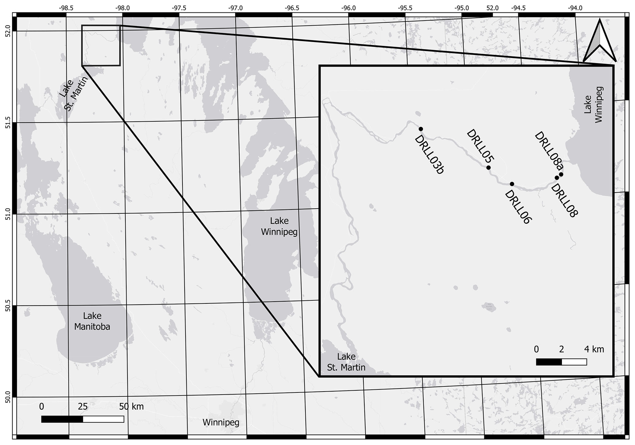
Figure 1Key map of the study location.
The Dauphin River is 52 km long and has steep, shallow banks that range between 110 and 160 m wide. The surficial geology of the area is composed of till with erratics, boulders, cobbles, and gravels observed throughout the channel. The most upstream 40 km of channel (Upper Dauphin River) has a mild slope (0.029 %) and is meandering. The bed composition of the Upper Dauphin River was observed to be primarily silt. The most downstream 12 km of channel (Lower Dauphin River) transitions into a well-defined riffle-pool system with a relatively high slope (0.16 %). Riffle sections in the Lower Dauphin River were observed to have a gravel bed with some boulders and erratics. Pool sections were observed to be silt bottomed. During winter ice formation, dramatic ice consolidation events, jams, and flooding have been reported by Wazney et al. (2018) on the Lower Dauphin River. Lake Winnipeg water levels can have a significant effect on the most downstream 2 km of this reach, which is typically where the largest toe of the ice jam would form.
2.2 Flow resistance
Surface roughness is an important parameter in the prediction of fluid flow along solid boundaries. This roughness creates drag along fluid boundary layers, generating the logarithmic fluid velocity distribution observed in open channel hydraulics. Rougher surfaces have been shown to exhibit greater flow resistance; however, it is not straightforward to quantify non-uniform, three-dimensional roughness elements. Nikuradse (1950) helped develop the concept of roughness height through equivalent sand grain roughness representing the height of sand particles fixed to the inside of pipes. More recently, an extensive discussion of methods used to represent the roughness of a heterogeneous three-dimensional surface layer from a surface profile was provided in Gadelmawla et al. (2002). Many of these methods involve statistical analysis of the entire sample or some subset of the sample (i.e. peaks, valleys, etc.). Gomez (1993) used the difference between peaks and a locally derived average bed surface for the investigation of gravel bed roughness. Nikora et al. (1998) recorded surface data derived from natural gravel point bars and found that the second-order moment of the frequency distribution yielded a suitable estimate of roughness height when compared to in situ field measurements. Aberle and Nikora (2006) also investigated higher-order statistics but confirmed the use of sample standard deviation (SD) as an appropriate representation of gravel bed roughness height. For non-normal data, the interquartile range (IQR) is a more suitable representation of the spread of the data.
For uniform flow conditions, Manning's equation is used to relate the discharge in an open-water or ice-covered channel to the water level. Flow resistance in this equation is introduced using Manning's n, which can be estimated from the roughness height of the channel boundary (in addition to many other modes of flow resistance that are outside the scope of the current study). Equation (1) shows a widely used quantitative method of estimating Manning's n from roughness height (D [m]) measurements proposed by Strickler (1923). Strickler suggested a value of cn=0.047 for general use, but this can be adapted for specific applications (Sturm, 2001).
Fluvial ice formation has a significant impact on the roughness characteristics of northern rivers. Ice covers increase hydraulic resistance in fluvial systems by replacing the relatively friction-free air–water boundary with a rougher ice–water boundary. This expands the wetted perimeter of the channel and, if the ice cover completely bridges the channel, may or may not pressurize flow. The added source of roughness and constriction of flow results in upstream staging (Beltaos, 2013). As with estimates of channel boundary roughness, ice roughness can also be judged qualitatively based on general observations with some success. The Nezhikhovskiy (1964) equation is a widely used empirical formula that provides a quantitative estimate of ice roughness in the form of Manning's n, as illustrated in Eq. (2). In this equation, ni is the Manning's n of the underside of the ice cover and ti [m] is the ice thickness in metres. In both cases, the subscript i refers to parameters related to ice.
This relationship is based on measurements conducted on rivers in Russia several decades ago, and it has served well as an estimation tool for engineering applications. Using more complex data, Eq. (1) was adapted by Beltaos (2013) for use in the estimation of the roughness of newly formed ice jams, resulting in Eq. (3).
The value given for cn=0.095 has been determined to be representative for ice jams. Additionally, the inclusion of the hydraulic radius R [m] accounts for the fact that the roughness elements of ice jams are often of such magnitude as to increase relative roughness to the point where it has a significant impact on the hydraulic radius. This relationship is only valid for newly formed ice jams; immediately after formation, the ice is subject to shear forces from the water flowing underneath, which slowly smoothens the subsurface of the ice cover (Ashton, 1986).
2.3 Remotely piloted aircraft photogrammetry
RPAs equipped with high-resolution digital cameras have been used extensively in the collection of near-surface photographic and topographic data (Colomina and Molina, 2014; Watts et al., 2012). They are smaller and more cost-effective than conventional aircraft, allowing for much more versatile data collection. Compared to manual surveying methods they can collect a greater volume of data in less time and greatly reduce risk to personnel. For the purposes of topographic data collection, the current common practice is to further process images collected with an RPA using structure from motion (SfM) photogrammetry (Fraser and Cronk, 2009). SfM photogrammetry is a technique that infers a three-dimensional structure from a series of overlapping, offset two-dimensional images (Westoby et al., 2012). Niethammer et al. (2012) used this method to monitor the progression of the Super-Sauze landslide, a task too dangerous to monitor manually. Eisenbeiss et al. (2005) employed RPA photogrammetry to document the layout of ancient ruins in Peru, which if done manually would have risked the integrity of the site. Hamshaw et al. (2019) found use for RPAs in the monitoring of riverbank erosion. RPAs were even used by Alfredsen et al. (2018) in the mapping of river ice in Norway.
Five field sites were selected in this study, their relative location along the bed profile of the Lower Dauphin River is illustrated in Fig. 2. Data were gathered during the winter months of 2017–2019. A relatively smooth, unconsolidated ice cover has been observed to form at DRLL03b in all previous study years, due to its low bed slope (0.029 %). Sites DRLL05 and DRLL06 exhibited substantial ice dynamics, as they are within the higher gradient (0.16 %) portion of the Lower Dauphin River (Wazney et al., 2019). Sites DRLL08 and DRLL08a had much milder water surface slopes, due to the backwater effect from Lake Winnipeg. The toe of an ice jam has formed in previous years near sites DRLL08a and DRLL08. These sites were selected in an effort to compare the efficacy of the RPA photogrammetry method on different ice conditions and to determine if the methods can distinguish roughness differences between sites.
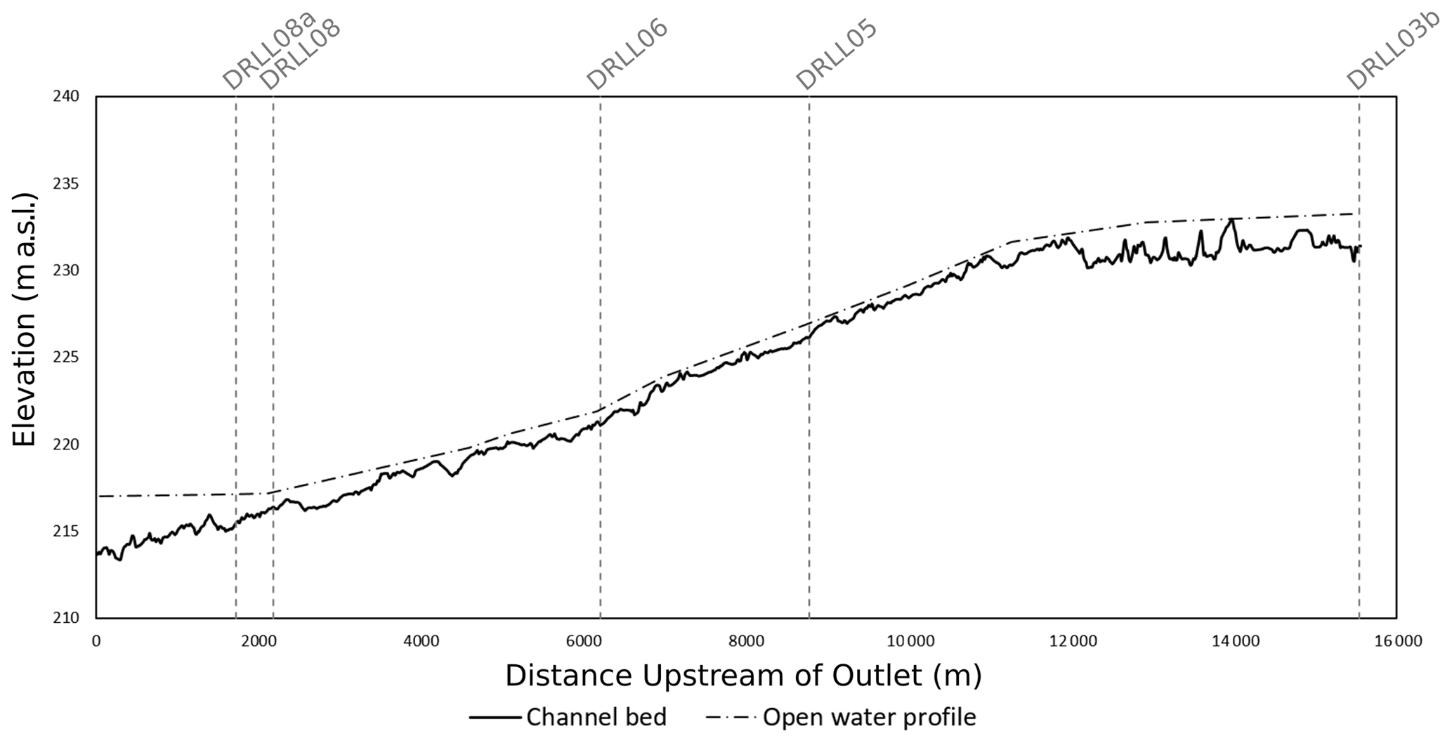
Figure 2Channel bed profile of the Lower Dauphin River, with selected study locations. Flow is 86 m3/s.
3.1 Field methods
3.1.1 Photogrammetry
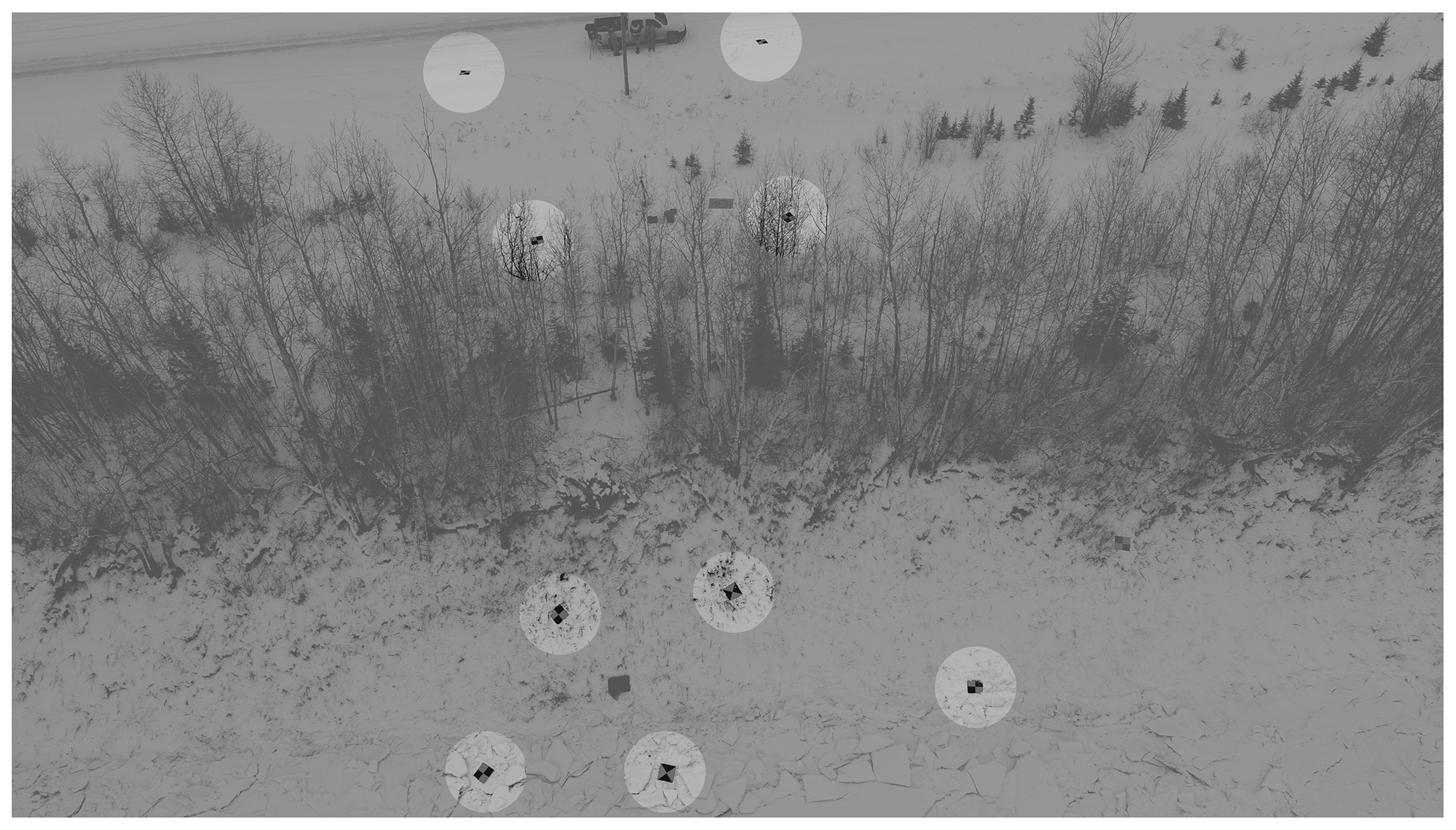
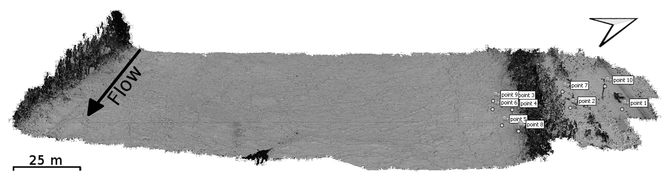
Remote monitoring of weather conditions informed the selection of field visit dates, with most data collected less than 1 week after the onset of ice formation on the study sites. A total of ten 1 m2 high-visibility medium-density fibreboard targets were distributed on the grounded ice near the left bank of each site and on snow near Provincial Road (PR) 513. A typical layout of targets is shown in Fig. 3, which illustrates how the targets are placed exclusively on the left bank of the river. The targets were grouped in this way since the right bank was inaccessible. Ideally, the targets would have been evenly distributed across the entire study area (Alfredsen et al., 2018; Gini et al., 2013). In Sect. 3.1.3, the effects of target distribution on digital elevation model (DEM) accuracy are tested.
After targets were placed, their centres were surveyed using a Leica Viva GS14® survey-grade real-time kinematic (RTK) Global Navigation Satellite System (GNSS) base-and-rover system, which is typically observed to have an in-field reported horizontal error of ≈2 cm and a vertical error of ≈3 cm. The Canadian Geodetic Vertical Datum of 2013 (CGVD2013) geoid was used in the recording of all surveyed elevations. Localization was assessed using a Manitoba Infrastructure (MI) benchmark located near DRLL03 and verified using the Natural Resources of Canada Canadian Spatial Reference System Precise Point Positioning (CSRS-PPP) service. Further benchmarks were established using the CSRS-PPP and “leap-frogging” to further benchmarks. In the 2019–2020 season, some RPA flights were completed without targets to allow for more flights to be completed during the field visit. A comparison between the representative metrics calculated from a DEM with and without geo-rectification is presented in Sect. 4.1.
Once all field personnel had finished active tasks, the RPA was launched, and field staff remained stationary for the duration of the RPA flight. A DJI Phantom 4 Professional® RPA was flown at an approximate altitude of 30 m, with overlapping photos taken every 10 m, at a 0∘ or 20∘ camera tilt. The on-board 20 megapixel camera had an 84∘ field of view with a 1 in. CMOS sensor. The RPA flight transected the river and included PR 513 and forest on the left and right bank, respectively. The RPA was flown only if wind speeds measured by a handheld digital anemometer were less than 36 km/h. Since light conditions could drastically impact the quality of images taken, the RPA was flown only during daytime and during clear or lightly overcast conditions. Typical capture dimensions of an RPA flight were 90 m in the stream-wise ordinate and 230 m across the river. During the 2019–2020 field season, the RPA mission planning application Pix4Dcapture® was used to plan and automate RPA flights over study areas. This greatly reduced the required flight time and produced similar (if not better) photo coverage.
3.1.2 Hydraulic parameters
Water pressure was recorded every 8 min at the study sites using Solinst Levelogger® Edge 3001 M5 pressure transducers and accompanying nearby Solinst Barologger® Edge 3001. The listed accuracy of these devices is ±0.003 m and ±0.05 kPa, respectively. These instruments were installed before the ice season began (typically October), removed for download and maintenance after the end of the ice season (typically April–May), and were then subsequently reinstalled for summer observations. During installation, the water surface was surveyed for use in post-processing to determine the absolute water surface elevation of the observations in metres above sea level (m a.s.l.). Additionally, the observed barometric pressure, converted to its equivalent depth of water, was subtracted from the pressure observations. The observed water level and previously measured channel bathymetry were used to estimate hydraulic radius at each of the study sites using a one-dimensional at-a-station hydraulic model based on Manning's equation.
During the 2019–2020 field season, holes were drilled in the ice cover at safe locations to determine ice thickness; however, not all locations allowed such convenient means of measurement. Ice thickness measurements of a rough, consolidating ice cover are impossible to conduct, and thus indirect measurement procedures were necessary, depending on the local conditions. In some cases, when it was clear that the ice cover was comprised of one or two layers of ice pans of known dimension, ice thicknesses were estimated through visual observation and photographs taken by stationary trail cameras. For highly consolidated thick ice covers, mid-winter RTK surveys were conducted to measure top of ice along the Lower Dauphin River. Lateral ice transects were conducted at locations where ice became grounded. The previously surveyed ground elevations were subtracted from these top-of-grounded-ice measurements to provide estimates of ice thickness. Late in the winter (typically February) after a stable ice cover had formed, a top-of-ice elevation survey was undertaken along the Lower Dauphin River using the base-and-rover system. Truncated transects of ice thickness were also surveyed at locations where ground elevation had previously been surveyed. A transect was performed at the DRLL06 and DRLL05 sites but not at DRLL08 due to safety concerns. During the 2019–2020 field season, holes were drilled in the ice cover at safe locations following established safe work procedures to determine ice thickness.
3.1.3 Field accuracy tests
There was a need to quantify the impact of the required ground control grouping on the left bank of the study area. The field methods described in Sect. 3.1.1 were repeated at River's Edge Nursery in La Barriere, Manitoba. A fully dry land study area of equivalent size to typical study areas flown at the Dauphin River was delineated, and 15 targets were distributed. The targets were conceptually grouped into three areas: typical, middle, and end. The “typical” group represented a target distribution that was generally produced during fieldwork at the Dauphin River sites. The “middle” and “end” target groups were supplemental and would be added or subtracted from the photogrammetry analysis to test their respective impacts on DEM accuracy. The distribution of targets in the study area is represented in Fig. 4. Finally, after the RPA flight was conducted, 10 independent and unmarked locations were captured by RTK-GNSS survey as a check for accuracy in subsequent data analysis.
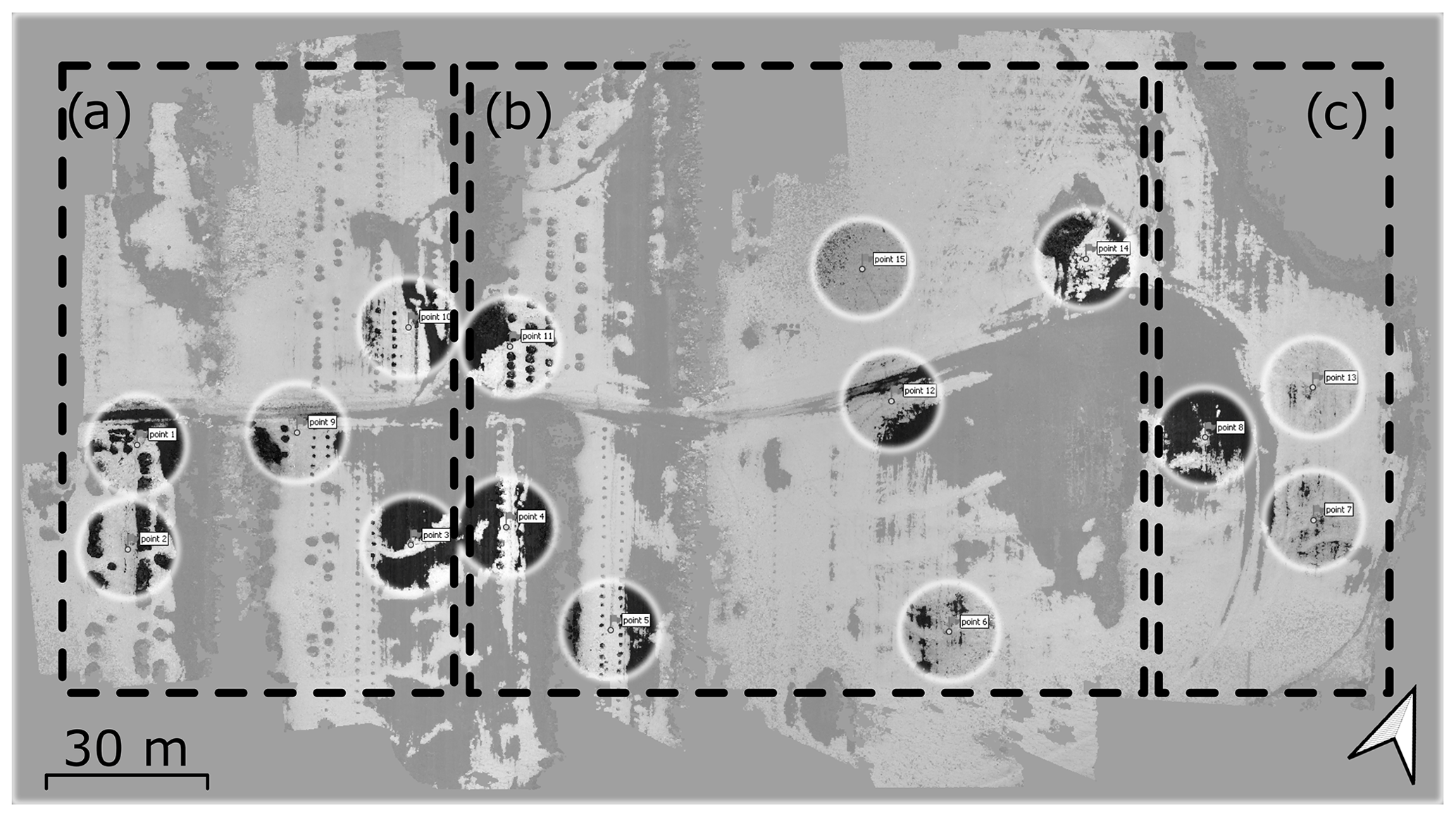
Figure 4Accuracy test experimental setup: (a) typical, (b) middle, (c) end.
3.2 Laboratory methods
3.2.1 Photogrammetry
The photogrammetry processing software selected for this study was PhotoScan Professional® from AgiSoft LLC. Gini et al. (2013) compared their custom research-grade photogrammetry algorithms to results obtained from Pix4UAV Desktop® and PhotoScan Professional®. Their findings suggested that these commercial packages performed similarly to their software, with PhotoScan Professional® performing somewhat better than Pix4UAV Desktop®. PhotoScan Professional® is also considered to be a relatively fully featured and complex (Eltner and Schneider, 2015) tool compared to other options.
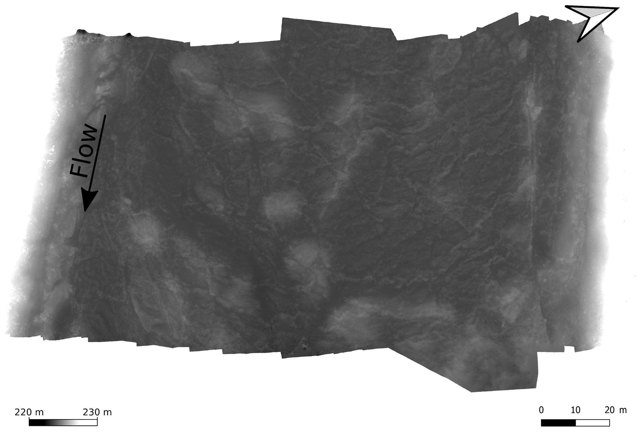
Images were imported into PhotoScan Professional®, and aligned to create a sparse point cloud of tie points. Where targets were used, they were identified in all images containing them, and their coordinates were imported to provide geo-rectification of the resultant point cloud. A dense point cloud was then generated, followed by a DEM. An example point cloud consisting of ≈15 million points and the corresponding DEM are shown in Figs. 5 and 6, respectively.
3.2.2 Accuracy testing
The impact of placing all control points on an extreme end of the study area was tested through a detailed trial on an open field. Groups of targets were used as input to the photogrammetry software, and the resultant DEMs were compared to the 10 independent survey points. The DEM generated using all available targets was assumed to be the most correct representation of the land surface, against which all other target groupings were compared. A maximum acceptable vertical difference of 0.03 m between the DEMs and the independent survey points was adopted. This value was chosen based on the typical error observed in the data gathered by the RTK GNSS base-and-rover system. This system was the limiting factor for accuracy in this study since it was the tool which informs the absolute spatial position of all field equipment. The following target scenarios were tested: “all points”, utilizing all ground control targets; “typical points”, using all the targets identified in the typical subset; “three points”, using a subset of three targets from the typical subset; and “two points”, using a subset of two targets from the typical subset. In the two- and three-point tests, the most spatially distributed targets within the typical subset were selected. An additional test was required to determine if systemic errors were introduced in DEMs generated without the use of geo-rectification targets. This scenario is referred to as the “no points” case. Data collected at site DRLL06 on 13 November 2019 were prepared with and without the inclusion of control point data. A maximum acceptable error of 5 % was adopted to evaluate the results of this test.
3.2.3 Roughness characterization
To avoid unwanted influences in the surface slope and texture, a 50 m2 subsample from the centre of the river was taken, which excluded all overbank objects and sections of the ice cover that were near to the bank. Additionally, a three-dimensional plane of best fit linear model (LM) was found for each sample and then subtracted from the surface data. The goal of this was to normalize each dataset, setting the average surface elevation to 0 and removing the river slope from the sample data. Gadelmawla et al. (2002) noted that the average surface elevation is the most commonly used and most sensible reference standard from which to assess roughness height. By shifting the elevation data down to a base elevation of 0 and removing unwanted patterns, each data point was transformed from an elevation to a roughness height.
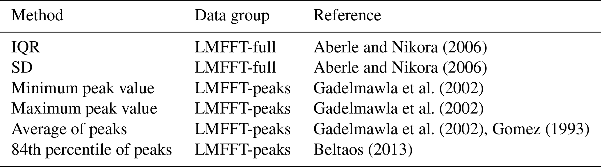
A two-dimensional fast Fourier transform (FFT) was then applied to each subsample, with the goal of filtering the input data and removing other surface trends beyond those addressed with the plane of best fit. The combination of the LM and FFT adjustment and filtering processes will be referred to as LMFFT. Through an analysis of dominant frequencies it was found that the lowest frequencies (<1 m−1) had the largest amplitudes, while the highest-frequency signals (>5 m−1) had the lowest amplitudes. A bandpass filter constructed with a low-pass value of 0.08 m was generally found to produce the best results. The high-pass component of the filter was adjusted through extensive iterative visual analysis of the image. High-pass cutoff values that were too aggressive caused obvious edge distortion, while values that were too conservative caused insufficient trend removal. The chosen high-pass wavelength cut-off values for all images ranged from 70 to 70.5 m. Figure 7a and b show the DEM before and after the application of this filter.
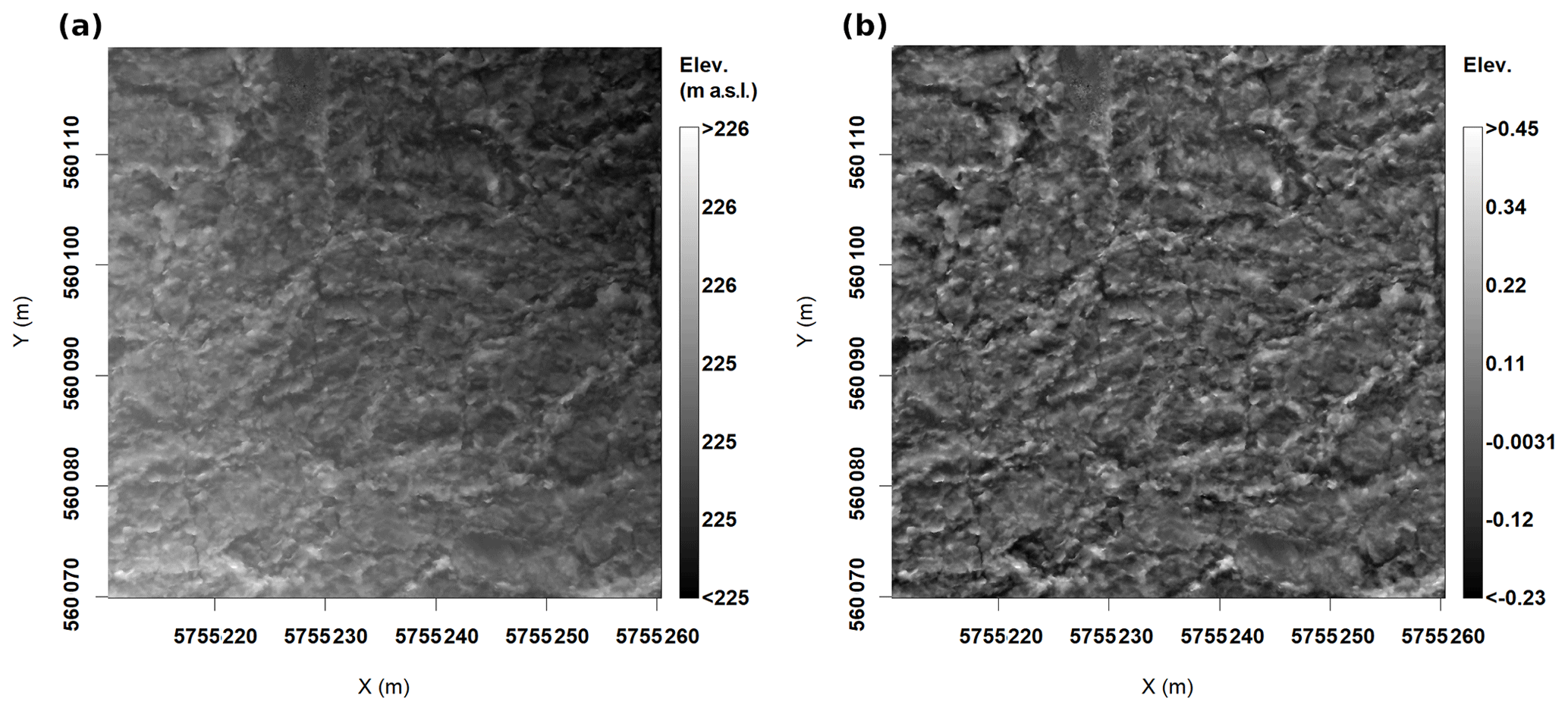
Figure 7Summary of impacts of filtering through Fourier analysis for DRLL06, 13 November 2019: (a) original ice surface DEM and (b) LMFFT-processed ice surface DEM.
A representative value of roughness height was required from each dataset for further analysis and comparison. Based on a review of relevant literature in the fields of photogrammetry, fluvial geomorphology, and roughness characterization, various statistical methods for roughness height characterization were considered, and several were chosen for further consideration in this study (Table 1). The full two-dimensional processed roughness height data, hereafter referred to as LMFFT-full, was then further analysed to create a second dataset that was comprised of only peak values of roughness height. This dataset, called LMFFT-peaks, was developed by extracting peak roughness heights using a three-dimensional implementation of the “peakpick” algorithm (Weber et al., 2014) available in the R programming language.
Aberle and Nikora (2006)Aberle and Nikora (2006)Gadelmawla et al. (2002)Gadelmawla et al. (2002)Gadelmawla et al. (2002)Gomez (1993)Beltaos (2013)Table 1Selected statistical metrics used to quantify RPA-measured ice surface roughness.
Once the various metrics of roughness height at each site were determined using the LMFTT-full and LMFTT-peaks datasets, the corresponding hydraulic radius for each site was determined using a simple one-dimensional hydraulic model based on Manning's equation. The model used the observed water level, estimated ice thickness, surveyed channel cross section, and an assumed specific gravity of ice of 0.916. Equation (3) was then used to calculate the RPA-measured ice surface Manning's n for each site.
In addition to a numerical characterization of roughness, a qualitative classification of roughness type was undertaken using k-means clustering, which is the most commonly used clustering approach (Jain, 2010). The input data were IQR and kurtosis of the LMFFT-full and LMFFT-peaks data and the median of the LMFFT-peaks data. Mean and median of the LMFFT-full data were excluded since they were set to 0 through the LMFFT process. Interestingly, the kurtosis was found to be a more useful metric for this analysis than the mean, standard deviation, or skewness. Since they was used in the computation of kurtosis, SD and skewness were removed from both datasets. The data were then mean-centred, and the optimal number of clusters was determined using the average silhouette method. The Euclidean distance formula was used in determination of the k-means clustering.
3.2.4 Roughness comparison
The RPA-measured ice surface Manning's n values from each site and using each of the roughness metrics were compared to Manning's n values computed using the commonly used Nezhikhovskiy equation (Eq. 2), as it has been found to make reasonable predictions of flow resistance of the underside of an ice cover. A similar comparison between RPA-measured ice surface Manning's n and the site ice thickness was also made. This was undertaken since ice thickness is the sole input parameter of the Nezhikhovskiy equation and could perhaps provide another perspective on the data. A linear regression was computed for the data in each plot. The quality of regressions were evaluated using the correlation coefficient (R2), F statistic (F), p value (p), and root-mean-square error (RMSE) values. The p value corresponds to the probability that the data show a significant trend through random chance and not an actual relationship. The criteria for significance in the p value was set to α≤0.05. The F value is a component of the p value and is another method of testing the significance of a linear regression when compared to its critical value Fcrit, which is calculated in Sect. 5.2. The validity of using linear regression modelling with these data was evaluated by testing the normality of residuals using the Shapiro–Wilk test for normality (p>0.05). This test was selected due to its wide usage in data analysis and its superior power compared to many other widely used normality tests (Razali and Wah, 2011). Q–Q plots of residuals were used to confirm the test statistics.
4.1 RPA performance
The RPA chosen for this study performed well during all field visits in various weather and cloud conditions. In extreme cold (−20 ∘C and below) the RPA performed all functions well, although the battery life was reduced by approximately 50 %. It was found that the RPA had to be powered on in a warm area, such as the heated cab of the field vehicle. Once powered on, it could then be placed outside for normal operations.
RPA photogrammetry performed very well across a variety of scenarios in the land-based field accuracy tests. The worst observed DEM accuracy was found in the two points scenario, with an average vertical difference of 6.30 m calculated between the DEM and the 10 independently surveyed test points. The three points, typical points, and all points scenarios all had the same average vertical difference of 0.03 m. These three scenarios were all within the acceptable vertical difference criteria of 0.03 m identified in Sect. 3.2.2. The maximum error of the DEM was determined to be the sum of the expected vertical accuracy of the RTK-GNSS unit, 0.03 m, and the observed vertical difference between the DEMs and surveyed locations, 0.03 m, for a total expected error of 0.06 m. The results of the no points test case, which sought to determine if a lack of geo-rectification targets introduces systemic errors into the DEM data, are presented in Table 2.
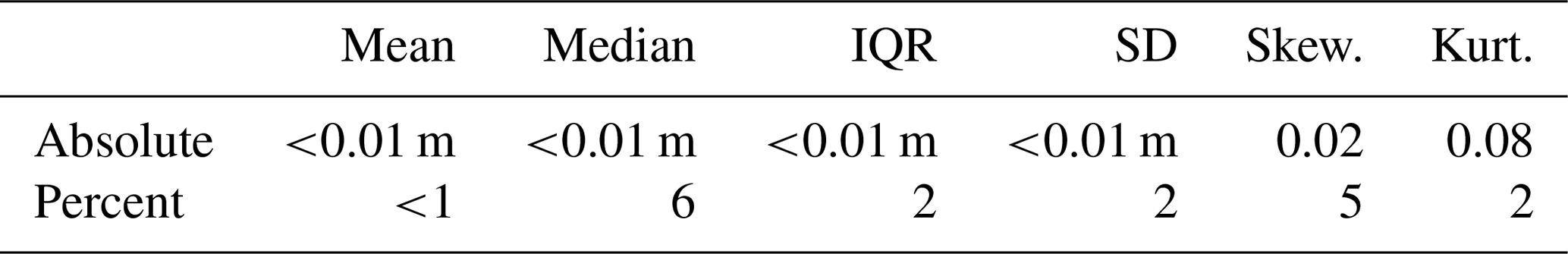
Table 2Percent and absolute difference between various statistical metrics computed from geo-rectified and non-geo-rectified (no ground control points) DEMs produced from data collected at DRLL06, 13 November 2019.
4.2 Dauphin River results
During the 2018–2019 and 2019–2020 field seasons, the Dauphin River experienced much lower flows than those observed in the previous few years. The mean seasonal flow between November and March for each season was 74 and 90 m3/s for 2018–2019 and 2019–2020, respectively, compared to 178 and 195 m3/s in 2016–2017 and 2017–2018, respectively, although in prior years lower flows were noted. This resulted in notably thinner ice covers, more thermal ice growth, and less extensive ice jamming than was reported by Wazney et al. (2018). The average values of observed ice thickness reduced from 2.9 m at site DRLL05 and DRLL06 in 2017–2018 to 1.8 and 0.8 m in 2018–2019 and 2019–2020, respectively.
4.2.1 Statistical properties of ice roughness height distributions
Several different forms of ice roughness were observed in DEMs produced using RPA photogrammetry. Figure 8 illustrates three different ice roughness forms observed at a single site, and their appearance in cross section along the indicated transects. The “rough” form of ice roughness was classified visually as any type of ice formed by the accretion and consolidation of frazil pans or broken pieces of border ice. The “smooth” form of ice roughness was classified as ice that appeared to have formed under quiescent conditions from a combination of transported and thermally grown ice that did not consolidate. Ice that exhibited pressure ridges on otherwise smooth ice was termed “ridged”.
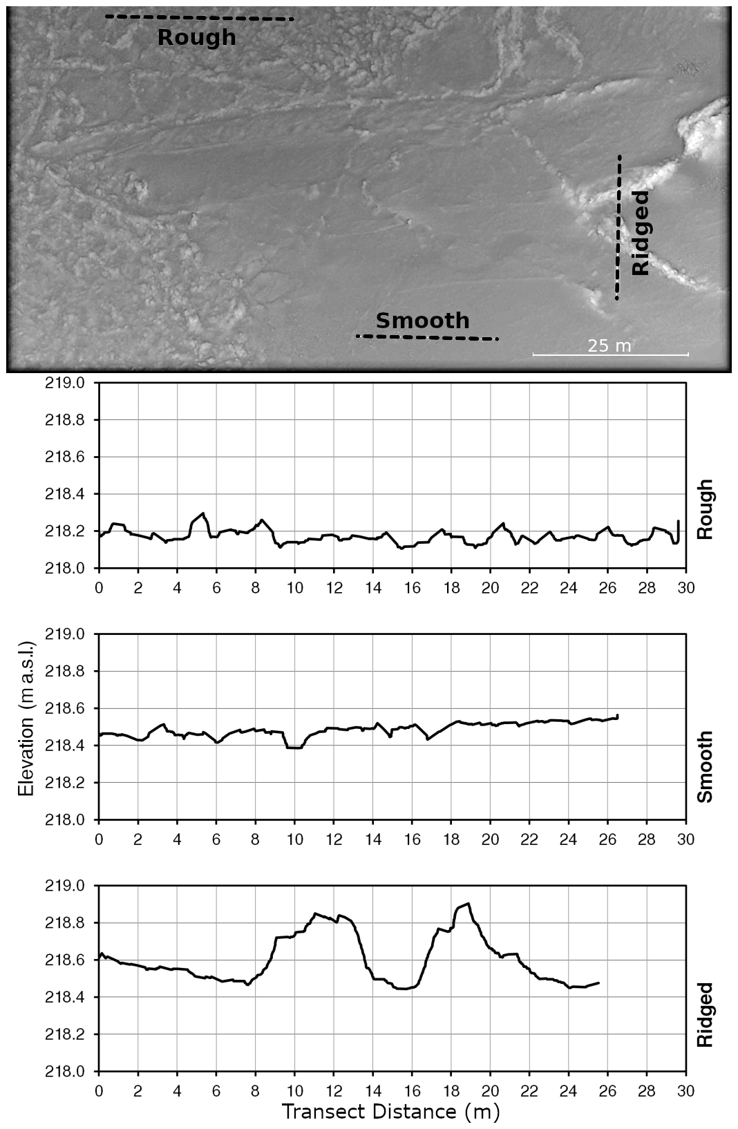
Figure 8Examples of three types of roughness observed in ice surface roughness samples along the indicated transects (dotted lines) at DRLL08a, 13 November 2019.
Two samples were observed to contain ridged ice, both of which occurred at site DRLL08a on 23 November 2017 and 23 November 2019. Ridged ice presented a unique situation for the evaluation of ice roughness based on surface ice characteristics. In sea ice, it is generally the case that the height of an observed pressure ridge above the ice cover (sail) is less than the depth to which the ridge extends below the ice cover (keel) (Johnston et al., 2009). In the fluvial setting this relationship is unknown, potentially complicating the hypothesis of this work. Therefore, samples exhibiting pressure ridge formations were discarded from subsequent comparisons between calculated ice roughness and k-means clustering. However, these data were retained for the general discussion of surface ice roughness characteristics found in Sect. 5.3.
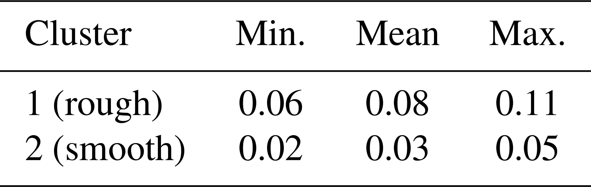
Cluster analysis was conducted using k-means clustering. The optimal number of clusters was found to be two when using average silhouette analysis. Table 3 illustrates the grouping of clusters in the data. The within cluster sum of squares was found to be 5.44 and 11.96 for clusters 1 and 2 respectively.

5.1 Accuracy of the RPA photogrammetry method for fluvial ice analysis
The results of the dry-land RPA photogrammetry accuracy test showed that if three or more targets were used, vertical differences of no more than 0.03 m were observed between resultant DEMs and independently surveyed points. This amount of vertical difference was deemed acceptable when compared to the maximum acceptable vertical difference of 0.03 m established in Sect. 3.2.2. No excessive tilt was observed in DEMs as a result of grouping targets on one side of the study area. AgiSoft PhotoScan Professional® appeared to be able to find an adequate number of tie points between images principally comprised of snow.
As described in Eltner et al. (2016), systemic errors causing deficiencies in DEM accuracy differ due to local-scale errors causing deficiencies in DEM precision. Systemic errors include those incurred by improper sampling technique and by limitations in the analysis. These errors were largely assumed to have been handled to the maximum extent possible in this research by the automated processes in AgiSoft PhotoScan Professional®. Eltner and Schneider (2015) found that AgiSoft PhotoScan Professional® also performed well in reproducing the texture of complex natural surfaces. Direct comparisons could not be made in this research between the naturally occurring ice surfaces and the RPA photogrammetry reproductions. However, the magnitude of such results as the maximum ice peak value matched visual observations and field notes. The accuracy test performed at the La Barrier field site confirmed that with appropriate ground control points this method could accurately reproduce snow-covered land surfaces. It also showed that the method could precisely reproduce features of the same order of magnitude as the chunks of ice expected to be measured on the Dauphin River.
Comparison of geo-rectified and non-geo-rectified DEMs yielded deviations for most metrics well within the 5 % threshold. The percent difference of the median was greater than 5 %; however, its absolute deviation was <0.01 m, which is much less than the maximum vertical error (0.06 m). These results confirm that geo-rectification was not strictly necessary for the analysis of surface ice roughness, since the analysis is principally concerned with surface variation rather than absolute location and orientation. However, geo-rectification would be necessary for most other applications of RPA photogrammetry of ice surfaces, such as those proposed in Sect. 5.4.
5.2 Comparison of ice roughness estimates
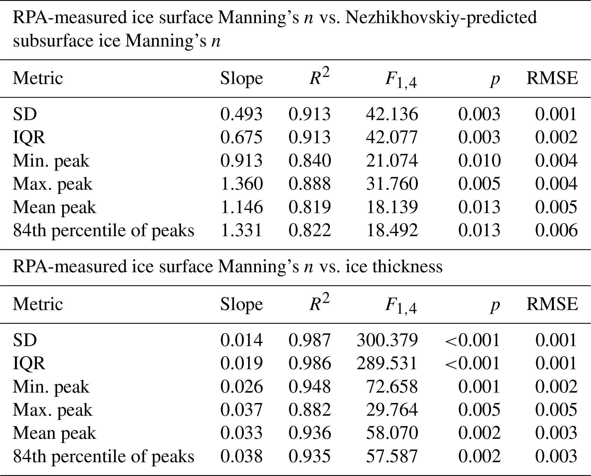
It was unclear which statistical metric would produce the most representative value of roughness height for the LMFFT-full and LMFFT-peak data. Since this has not been attempted in the field of fluvial ice research, a total of six potential options for the calculation of roughness height were selected, and once converted to Manning's n using Eq. (3), they were compared to the Nezhikhovskiy-predicted subsurface ice Manning's n (Fig. 9) and ice thickness (Fig. 10). A linear regression was attempted in each plot, and the corresponding statistical parameters are presented in Table 4. The reported F statistic (F1,4) has 1 and 4 degrees of freedom for the numerator and denominator, respectively. Using the significance value of α≤0.05 established in Sect. 3.2.4, a value of Fcrit of 0.0045 was found. Values of F1,4 greater than this value indicate a significant relationship.
Figure 9 highlights the fact that the Nezhikhovskiy-predicted subsurface ice Manning's n was generally greater than the RPA-measured values and plotted over a fairly narrow range. Most RPA-derived roughness values did not fall on the 1:1 line, indicating that the RPA-measured ice surface Manning's n was not identical to the values predicted using a common empirical relationship. It should be noted, however, that ice cover with relatively high RPA-measured surface ice Manning's n had high Nezhikhovskiy-predicted subsurface ice Manning's n and vice versa.
5.2.1 RPA-measured ice surface Manning's n vs. Nezhikhovskiy-predicted subsurface ice Manning's n
The p statistic found that all relationships were significant (α≤0.05) in this comparison. The F1,4 statistic exceeded the Fcrit value of 0.0045 in all cases. All metrics illustrated strong correlation with high R2 values and low RMSE. The SD and IQR performed the best of all metrics, with the highest R2 values and lowest p and RMSE results. These results indicate the ice roughness values derived from RPA photogrammetry were proportional to roughness values predicted using the Nezhikhovskiy equation.
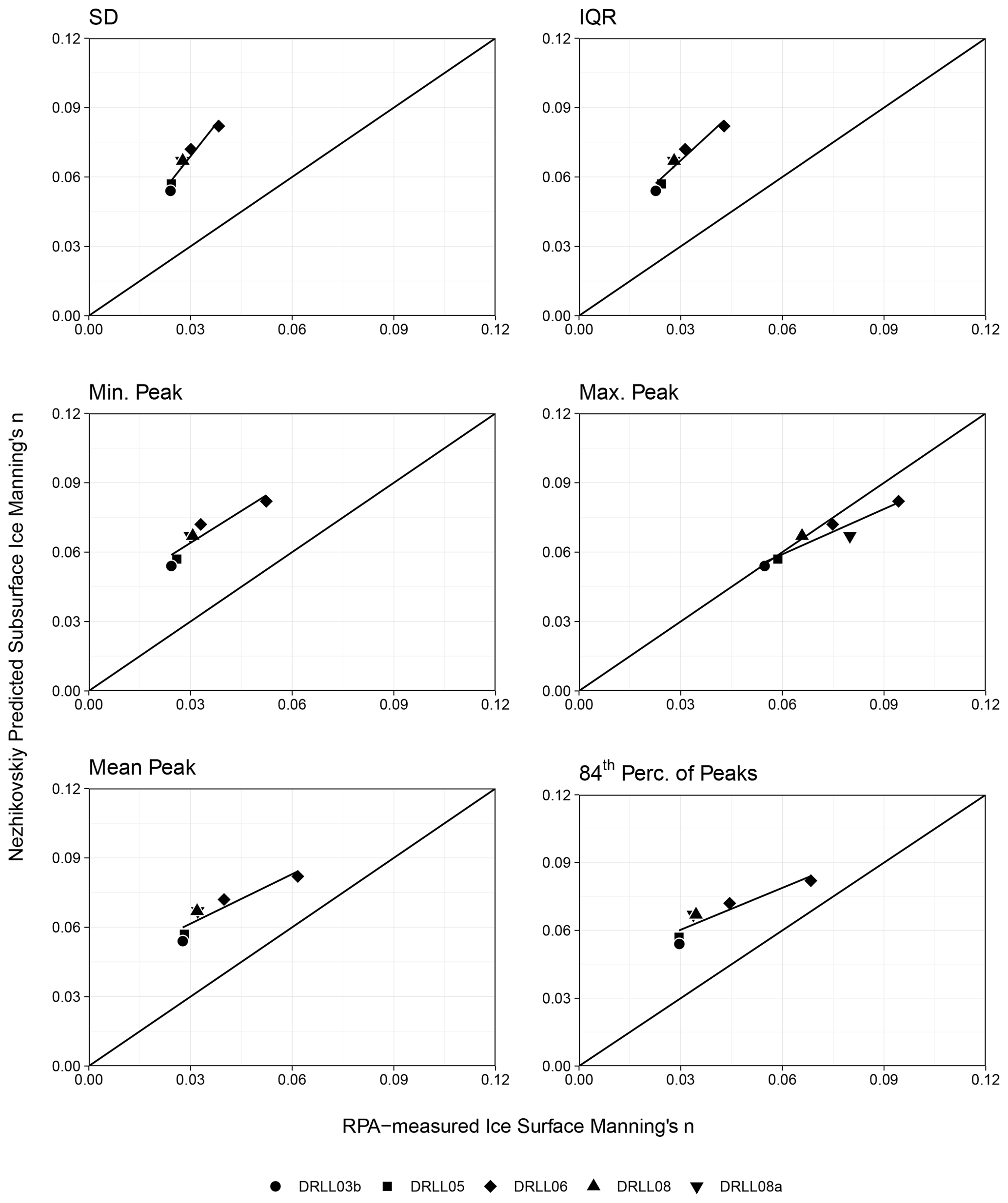
Figure 9Comparison of RPA-measured surface ice Manning's n calculated from various statistical metrics or roughness height to Nezhikhovskiy-predicted subsurface ice Manning's n.
5.2.2 RPA-measured ice surface Manning's n vs. ice thickness
Since the only input parameter for the Nezhikhovskiy equation is ice thickness, the RPA-measured ice surface Manning's n values were compared directly to their associated ice thickness measurements (and estimates) as shown in Fig. 10. All metrics of roughness height taken from the DEMs were found to generate RPA-measured ice surface Manning's n values that were strongly correlated with ice thickness. The corresponding regression statistics are reported in Table 4. The IQR and SD again performed the best, with the highest R2 value and lowest RMSE, although all metrics performed exceptionally well. The p statistic showed that all relationships were significant (α≤0.05), and the F1,4 statistic exceeded the Fcrit value of 0.0045 in all cases. Further research would be required to determine if this relationship may be used to estimate ice thickness based on observed surface roughness.
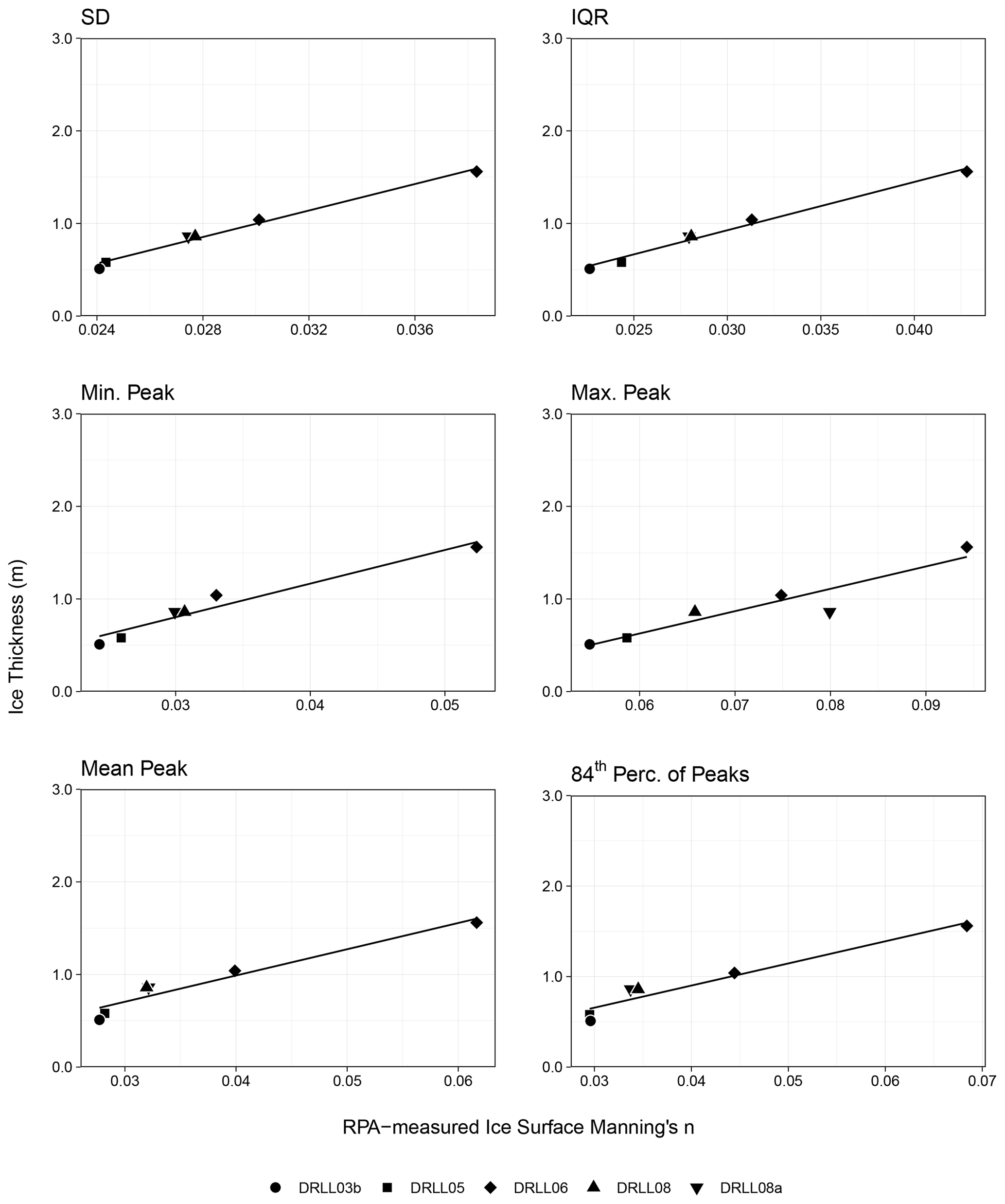
Figure 10Comparison of RPA-measured ice surface Manning's n calculated from various statistical metrics to site ice thickness.
5.3 Statistical properties of ice surface roughness heights
All observations at site DRLL06 were found to belong to cluster “1”, while observations at site DRLL03b, DRLL05, DRLL08, and DRLL08a belonged to cluster “2”. The cluster results were enforced by observations taken at the time of sample collection. The samples were broadly separated into two groups corresponding to the visual extent of rough or smooth ice, as defined earlier in this section. Samples in cluster 1 were observed to be rough, while samples in cluster 2 were observed to be smooth. Considering the SD of the LMFFT-full data, which was the best performing metric in Sect. 5.2, Table 5 provides the minimum, mean, and maximum values of the sites within each identified cluster. Cluster 1, the rough cluster, corresponded to ice surfaces with higher SD values, while cluster 2, the smooth cluster, has lower SD values. The range of values are mutually exclusive, indicating a strong divide between the two groups.
Table 5Minimum, mean, and maximum values of surface SD for clusters.
For each site, the LMFTT-full data as well as the LMFTT-peaks data subset were analysed in detail. Figure 11 presents typical examples of rough, smooth, and ridged ice. The rough and smooth samples corresponded to sites from each of the rough and smooth clusters. The ridged samples were those identified in Sect. 4.2.1. To the authors' knowledge this is the first time that roughness of a river ice cover's surface has been quantified in such detail. The LMFTT-full histograms were observed to have distributions that appeared Gaussian in a qualitative sense, as shown in Fig. 11. Despite the appearance, all distributions failed the Shapiro–Wilk normality test, with p≪0.05, using a randomized subsample (≈5000 points) of the data. Considering the distribution of peak values only, all sites exhibited clearly non-normal distributions that were heavily biased to the extreme left of the chart. This was interpreted to mean that the majority of peaks were small compared to the maximum peak values.
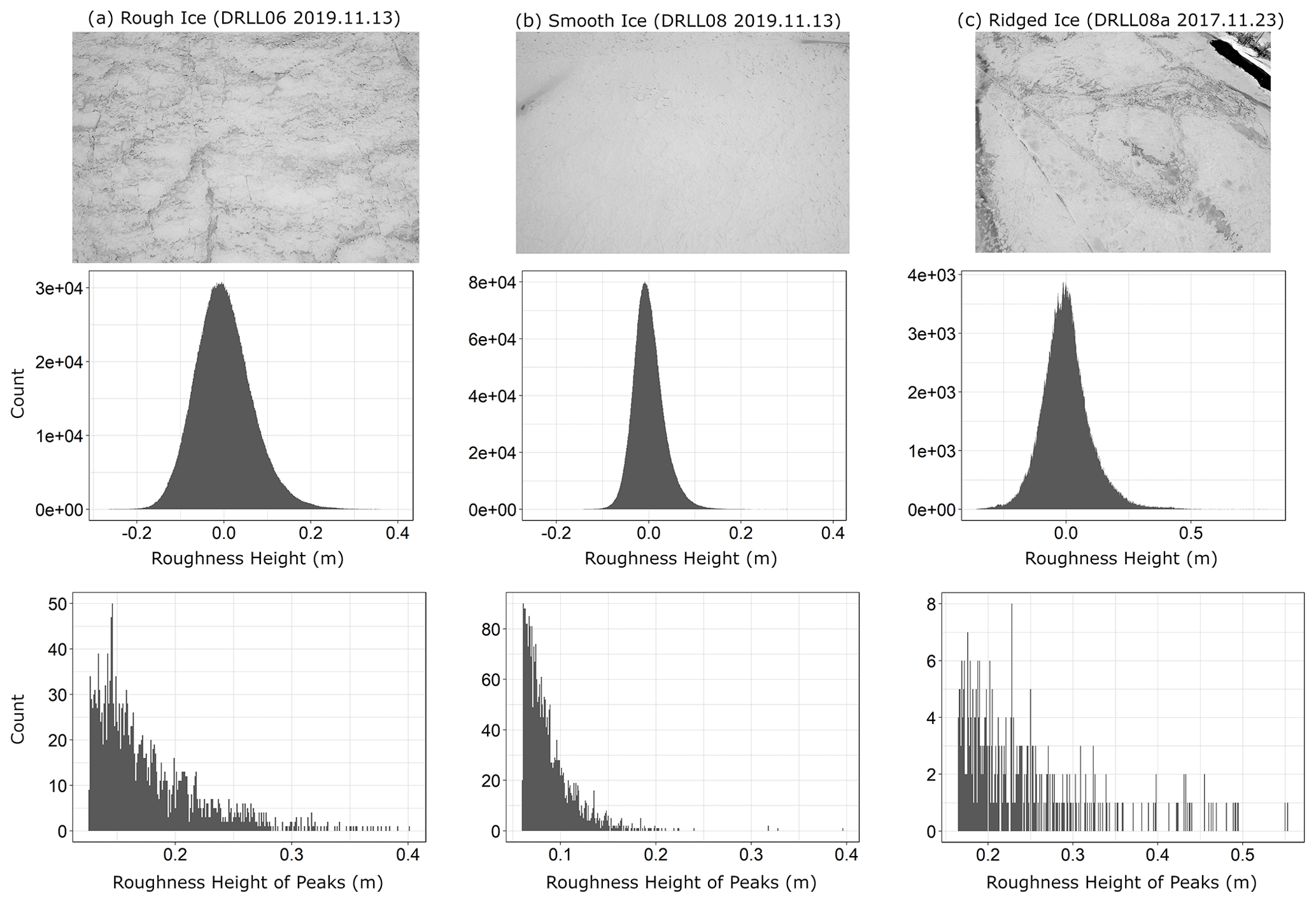
Figure 11Comparison of representative roughness height histograms across three identified ice types.
It was noted that the rough and smooth samples differed primarily in the width and height of their distributions. The rough samples tended to have wider distributions with a lower peak count, while the smooth distributions had a higher peak count and a narrower distribution of roughness heights. The distributions of peak roughness height also differed, with the rough samples having more larger peaks than the smooth samples. The ridged samples exhibited more irregular distributions than the rough or smooth cases but were more similar to rough distributions in being wider and having lower peak counts than smooth distributions.
5.4 Alternative uses for RPA photogrammetry
A common problem in river ice elevation surveys is the selection of a single, representative value to define the average ice surface elevation in a given area, especially when the ice cover is quite rough. It is up to the practitioner to use their best judgement to visually select a single representative point to survey while walking along the river bank, and the simple choice of resting the survey rod on the top of a piece of ice or the bottom of that same piece of ice will cause the local ice elevation measurement to vary considerably. During massive ice jam events, this field task is dangerous and frequently impossible. The above research shows that RPA photogrammetry can be used to accurately survey ice areas for the purpose of observing local topography, with much lower risks to field personnel than traditional ice surveying methods. Once a geo-rectified DEM has been established, a representative ice elevation value of the entire rough ice surface can be determined using the LM approach introduced in Sect. 3.2.3. This analysis could be extended to examine shear walls and determine maximum ice elevation of a freeze-up jam after the fact.
The research presented in this work has developed novel methods for the capture and analysis of fluvial ice surface elevation and roughness data. Through field trials and controlled land-based experiments, it was determined that RPA photogrammetry produced an accurate digital representation of rough or smooth ice covers, with a maximum vertical error of 0.06 m if using three or more ground control points over a 200 m by 100 m area. For the sole purpose of roughness characterization, it was determined that geo-rectification was unnecessary using our equipment. The relatively inexpensive consumer-grade RPA was able to operate in harsh winter field conditions, with an approximately 50 % reduced battery life. For the first time in the river ice engineering field, the top-of-ice surface roughness has been quantified in detail using high-resolution RPA photogrammetry. A combination of linear processing and Fourier filtering were proposed, and bulk statistical properties of the ice roughness samples have been computed. Histograms of different ice types have been presented for the first time, and k-means clustering analysis has identified two distinct classes of surface ice roughness. Through evaluation of the statistical properties of the distribution of DEM heights observed via RPA photogrammetry, several interesting patterns were found. All distributions were found to be non-normal when evaluated with the Shapiro–Wilk normality test; however, they display a qualitatively normal appearance.
The hypothesis of this research, i.e. that the surface roughness of a newly frozen fluvial ice cover is indicative of subsurface roughness, was tested. When comparing the Nezhikhovskiy-predicted values to the RPA-measured values, all roughness height metrics produced significant relationships, many with R2>0.9. In this comparison IQR and SD had the lowest p values, highest R2 values, and lowest RMSE values. It can be concluded that even though the RPA-measured ice surface Manning's n was not equivalent to Nezhikhovskiy-predicted subsurface ice Manning's n, the correlations were strong enough to suggest that RPA-measured surface ice roughness and subsurface ice roughness increase in tandem.
Very strong positive correlation was observed between the RPA-measured surface ice roughness and ice thickness across all tested metrics. Once again the SD and IQR of the roughness height DEM were found to be the best metrics for roughness height, with the highest R2 and lowest RMSE and p values. This relationship also supports the hypothesis that surface ice roughness is related to subsurface ice roughness, since the data show that RPA-measured ice surface roughness increases with ice thickness and a widely used empirical formula predicts the same relationship. Future work should focus on increasing the number of field observations taken using these methods, across a wider range of ice roughness values and on different rivers of various size and flow conditions.
The methods presented in this research can conceivably be applied to further uses in the field of fluvial ice monitoring. For example, the high-resolution DEMs produced by this method can be used to determine a more representative spot measurement of ice elevation, which has the potential to significantly increase the accuracy of river ice jam profile plots. This could potentially improve ice jam numerical model development since model performance is consistently evaluated by comparing simulated jam profiles to measured ice jam profiles. Furthermore, shear walls may be captured and analysed in their entirety, even immediately after or during break-up. This research also presents a possible link between surface ice roughness and ice thickness, which may provide for a method of estimating ice thickness using RPA photogrammetry. The use of RPA photogrammetry for the monitoring of fluvial ice covers offers a quicker, safer, and cheaper alternative to any previous method of high-resolution topographic data collection, and its applications are open for development.
Data related to this study, including raw images, point clouds, and summary data, are available upon request from the corresponding author.
JE, SC, and AW developed the research plan and conducted fieldwork. JE processed all field data and developed all data analysis tools. JE and SC drew conclusions based on the results.
The authors declare that they have no conflict of interest.
Publisher's note: Copernicus Publications remains neutral with regard to jurisdictional claims in published maps and institutional affiliations.
This research has been supported by the Natural Sciences and Engineering Research Council of Canada (grant no. IRCPJ472185-13) and Manitoba Hydro (grant no. G274/P274).
This paper was edited by Nicholas Barrand and reviewed by two anonymous referees.
Aberle, J. and Nikora, V.: Statistical properties of armored gravel bed surfaces, Water Resour. Res., 42, W11414, https://doi.org/10.1029/2005WR004674, 2006. a, b, c
Alfredsen, K., Haas, C., Tuhtan, J. A., and Zinke, P.: Brief Communication: Mapping river ice using drones and structure from motion, The Cryosphere, 12, 627–633, https://doi.org/10.5194/tc-12-627-2018, 2018. a, b
Ashton, G. D. (Ed.): River and lake ice engineering, Water Resources Publication, Chelsea, Michigan, USA, 261–361, ISBN 0-918334-59-4, 1986. a
Beltaos, S. (Ed.): River Ice Formation, The Committee on River Ice Processes and the Environment, Edmonton, Alberta, Canada, 218–232, ISBN 978-0-9920022-0-6, 2013. a, b, c, d
Buffin-Belanger, T., Demers, S., and Olsen, T.: Quantification of under ice cover roughness, in: 18th Workshop on the Hydraulics of Ice Covered Rivers, CGU HS Committee on River Ice Processes and the Environment, Quebec City, QC, Canada, 2015. a, b
Chudley, T. R., Christoffersen, P., Doyle, S. H., Abellan, A., and Snooke, N.: High-accuracy UAV photogrammetry of ice sheet dynamics with no ground control, The Cryosphere, 13, 955–968, https://doi.org/10.5194/tc-13-955-2019, 2019. a
Colomina, I. and Molina, P.: Unmanned aerial systems for photogrammetry and remote sensing: A review, ISPRS Jounral of Photogrammetry and Remote Sensing, 92, 79–97, https://doi.org/10.1016/j.isprsjprs.2014.02.013, 2014. a, b
Crance, M.-J. and Frothingham, K. M.: The Impact of Ice Cover Roughness on Stream Hydrology, in: 65th Eastern Snow Conference, pp. 149–165, Fairlee, Vermont, USA, 2008. a, b
Dammann, D. O., Eicken, H., Mahoney, A. R., Saiet, E., Meyer, F. J., and George, J. C.: Traversing Sea Ice – Linking Surface Roughness and Ice Trafficability Trhough SAR Polarimetry and Interferometry, IEEE Journal of Selected Topics in Applied Earth Observations and Remote Sensing, 11, 416–433, https://doi.org/10.1109/JSTARS.2017.2764961, 2018. a, b, c, d
Eisenbeiss, H., Lambers, K., and Sauerbrier, M.: Photogrammetric recording of the archaeological site of Pinchango Alto (Palpa, Peru) using a mini helicopter (UAV), in: The world is in your eyes: CAA 2005: Computer Applications and Quantitative Methods in Archaeology, proceedings of the 33rd Conference, edited by: Figueiredo, A., pp. 175–184, 2005. a
Eltner, A. and Schneider, D.: Analysis of different methods for 3D reconstruction of natural surfaces from parallel-axes UAV images, The Photogrammetric Record, 30, 279–299, https://doi.org/10.1111/phor.12115, 2015. a, b
Eltner, A., Kaiser, A., Castillo, C., Rock, G., Neugirg, F., and Abellán, A.: Image-based surface reconstruction in geomorphometry – merits, limits and developments, Earth Surf. Dynam., 4, 359–389, https://doi.org/10.5194/esurf-4-359-2016, 2016. a
Fitzpatrick, N., Radić, V., and Menounos, B.: A multi-season investigation of glacier surface roughness lengths through in situ and remote observation, The Cryosphere, 13, 1051–1071, https://doi.org/10.5194/tc-13-1051-2019, 2019. a, b
Fraser, C. S. and Cronk, S.: A hybrid measurement approach for close-range photogrammetry, ISPRS Journal of Photogrammetry and Remote Sensing, 64, 328–333, 2009. a
Gadelmawla, E. S., Koura, M. M., Maksoud, T. M. A., Elewa, I. M., and Soliman, H. H.: Roughness parameters, J. Mater. Proc. Technol., 123, 133–145, https://doi.org/10.1016/S0924-0136(02)00060-2, 2002. a, b, c, d, e
Gerard, R. and Andres, D.: Hydraulic roughness of freeze-up ice accumulations: North Sasksatchewan River through Edmonton, 2nd Workshop on the Hydraulics of Ice Covered Rivers, Edmonton, Alberta, Canada, pp. 62–86, 1984. a
Gini, R., Pagliari, D., Passoni, D., Pinto, L., Sona, G., and Dosso, P.: UAV photogrammetry: Block triangulation comparisons, Internation Archives of the Photogrammetry, Remote Sensing and Spatial Information Sciences, XL-1/W2, 157–162, 2013. a, b
Gomez, B.: Roughness of Stable, Armored Gravel Beds, Water Resour. Res., 29, 3631–3642, 1993. a, b
Hamshaw, S. D., Engel, T., Rizzo, D. M., O'Neil-Dunne, J., and Dewoolkar, M. M.: Application of unmanned aircraft system (UAS) for monitoring bank erosion along river corridors, Geomatics, Nat. Haz. Risk, 10, 1285–1305, https://doi.org/10.1080/19475705.2019.1571533, 2019. a
Jain, A. K.: Data clustering: 50 years beyond k-means, Pattern Recogn. Lett., 31, 651–666, https://doi.org/10.1016/j.patrec.2009.09.011, 2010. a
Johnston, M., Masterdon, D., and Wright, B.: Multi-Year Ice Thickness: Knowns and Unknowns, in: Proceedings of the International Conference on Port and Ocean Engineering Under Arctic Conditions, pp. 969–981, 2009. a
Kirby, R. P.: Measurement of Surface Roughness in Desert Terrain By Close Range Photogrammetry, Photogrammetric Record, 13, 855–875, 1991. a
Nezhikhovskiy, R. A.: Coefficients of roughness of bottom surface on slush-ice cover, Soviet Hydrology, Washington, American Geophysical Union, Selected Papers 2, pp. 127–150, 1964. a, b
Niethammer, U., James, M., Rothmund, S., Travelletti, J., and Joswig, M.: UAV-based remote sensing of the Super-Sauze landslide: Evaluation and results, Eng. Geol., 128, 2–11, https://doi.org/10.1016/j.enggeo.2011.03.012, 2012. a
Nikora, V. I., Goring, D. G., and Biggs, B. J. F.: On gravel-bed roughness characterization, Water Resour. Res., 34, 517–527, 1998. a
Nikuradse, J.: Laws of Flow in Rough Pipes, Technical Memorandum 1292, National Advisory Committee for Aeronautics, 1950. a
Razali, N. M. and Wah, Y. B.: Power Comparisons of Shapiro0Wilk, Komolgorov-Smirnov, Lilliefors and Anderson-Darling tests, J. Stat. Model. Anal., 2, 21–33, 2011. a
Strickler, A.: Contributions to the Question of a Velocity Formula and Roughness Data for Streams, Channels and Closed Pipelines, Tech. Rep. 16, Swiss Department of the Interior, Bureau of Water Affairs, 1923. a
Sturm, T. W.: Open Channel Hydraulics, McGraw Hill, 2001. a
Watts, A. C., Ambrosia, V. G., and Hinkley, E. A.: Unmanned Aircraft Systems in Remote Sensing and Scientific Research: Classification and Considerations of Use, Remote Sens., 4, 1671–1692, https://doi.org/10.3390/rs4061671, 2012. a
Wazney, L., Clark, S. P., and Wall, A. J.: Field monitoring of secondary consolidation events and ice cover progression during freeze-up on the Lower Dauphin River, Manitoba, Cold Reg. Sci. Technol., 148, 159–171, https://doi.org/10.1016/j.coldregions.2018.01.014, 2018. a, b, c
Wazney, L., Clark, S. P., and Malenchak, J.: Effects of freeze-up consolidation event surges on river hydraulics and ice dynamics on the Lower Dauphin River, Cold Reg. Sci. Technol., 158, 264–274, https://doi.org/10.1016/j.coldregions.2018.09.003, 2019. a
Weber, C. M., Ramachandran, S., and Henikoff, S.: Nucleosomes are context-specific, H2A.Z-modulated barriers to RNA polymerase, Molecular Cell, 53, 819–830, 2014. a
Westoby, M. J., Brasington, J., Glasser, N. F., Hambrey, M. J., and Reynolds, J. M.: 'Structure-from-Motion' photogrammtery: A low-cost, effective tool for geoscience applications, Geomorphology, 179, 300–314, https://doi.org/10.1016/j.geomorph.2012.08.021, 2012. a
Yitayew, T. G., Dierking, W., Divine, D. V., Eltoft, T., Ferro-Famil, L., Rösel, A., and Negrel, J.: Validation of Sea-Ice Topographic Heights Derived From TanDEM-X Interferometric SAD Data With Results From Laser Profiler and Photogrammetry, IEEE T. Geosci. Remote, 56, 6504–6520, https://doi.org/10.1109/TGRS.2018.2839590, 2018. a