the Creative Commons Attribution 4.0 License.
the Creative Commons Attribution 4.0 License.
 | 17 Aug 2021
What is the surface mass balance of Antarctica? An intercomparison of regional climate model estimates
Nicolaj Hansen
Christoph Kittel
J. Melchior van Wessem
Cécile Agosta
Charles Amory
Fredrik Boberg
Willem Jan van de Berg
Xavier Fettweis
Alexandra Gossart
Nicole P. M. van Lipzig
Erik van Meijgaard
Andrew Orr
Tony Phillips
Stuart Webster
Sebastian B. Simonsen
Niels Souverijns
We compare the performance of five different regional climate models (RCMs) (COSMO-CLM2, HIRHAM5, MAR3.10, MetUM, and RACMO2.3p2), forced by ERA-Interim reanalysis, in simulating the near-surface climate and surface mass balance (SMB) of Antarctica. All models simulate Antarctic climate well when compared with daily observed temperature and pressure, with nudged models matching daily observations slightly better than free-running models. The ensemble mean annual SMB over the Antarctic ice sheet (AIS) including ice shelves is 2329±94 Gt yr−1 over the common 1987–2015 period covered by all models. There is large interannual variability, consistent between models due to variability in the driving ERA-Interim reanalysis. Mean annual SMB is sensitive to the chosen period; over our 30-year climatological mean period (1980 to 2010), the ensemble mean is 2483 Gt yr−1. However, individual model estimates vary from 1961±70 to 2519±118 Gt yr−1. The largest spatial differences between model SMB estimates are in West Antarctica, the Antarctic Peninsula, and around the Transantarctic Mountains. We find no significant trend in Antarctic SMB over either period. Antarctic ice sheet (AIS) mass loss is currently equivalent to around 0.5 mm yr−1 of global mean sea level rise (Shepherd et al., 2020), but our results indicate some uncertainty in the SMB contribution based on RCMs. We compare modelled SMB with a large dataset of observations, which, though biased by undersampling, indicates that many of the biases in SMB are common between models. A drifting-snow scheme improves modelled SMB on ice sheet surface slopes with an elevation between 1000 and 2000 m, where strong katabatic winds form. Different ice masks have a substantial impact on the integrated total SMB and along with model resolution are factored into our analysis. Targeting undersampled regions with high precipitation for observational campaigns will be key to improving future estimates of SMB in Antarctica.
- Article
(8531 KB) - Full-text XML
- BibTeX
- EndNote


The Antarctic ice sheet (AIS) is the largest body of freshwater on the planet and an important contributor to global sea level rise. It is also a significant part of the climate system, contributing freshwater to the ocean and with high relief that influences atmospheric circulation. Studies by Rignot et al. (2011, 2019) and Shepherd et al. (2018) showed the AIS to have had a net loss since at least 2002. Current estimates suggest that around 10 % of observed sea level rise since 1993 is from Antarctica; however that rate of contribution is also increasing (Oppenheimer et al., 2019). Most ice loss in Antarctica occurs as a result of submarine melting, that is melt at the water–ice interface underneath ice shelves, or by the calving of icebergs from ice shelves. Recent ice dynamics studies (DeConto and Pollard, 2016; Edwards et al., 2019; Sutter et al., 2016; Shepherd et al., 2018) have shown that there is potential for rapid ice sheet loss owing to ice sheet dynamics that are currently poorly understood, especially in West Antarctica. Ice sheet models of the AIS have thus largely concentrated on parameterizing sub-shelf and calving processes. However, surface mass balance (SMB), also known as climate mass balance (Cogley et al., 2010), is also of crucial importance in controlling the stability and evolution of the vast ice sheet. Changes in precipitation and increases in surface melt and run-off will change the mass balance and therefore both ice dynamics and the sea level rise contribution from Antarctica in the future. Moreover there has been disagreement between studies focused on the SMB contribution to the total mass budget of Antarctica and therefore the contribution to sea level rise (Scambos and Shuman, 2016; Zwally et al., 2015) that makes it essential to understand potential biases and uncertainties.
SMB is the difference between accumulation and ablation at the surface of a glacier. In Antarctica, accumulation is derived primarily from solid precipitation, but on local or regional scales wind-driven processes can have a significant effect on accumulation rates. Surface ablation in Antarctica is primarily a result of erosion and sublimation due to the high winds and generally dry atmosphere (Scambos et al., 2012; Das et al., 2013; Agosta et al., 2019), although increasing melt rates are documented in some areas (Stokes et al., 2019). In the future, a “Greenlandification” of the ice sheet climate is projected due to anthropologically induced climate change (Trusel et al., 2018). This will lead to more melt with more refreezing in the snowpack as well as increasing run-off.
It is important to distinguish between the continental grounded ice sheet and ice shelves when considering values for SMB integrated over a wider area, whether regional or continent-wide. Snowfall and melt on ice shelves is not directly relevant to sea level rise contributions as they are already floating, but precipitation and ablation on grounded parts of the ice sheet is. As the models used in this study by and large do not distinguish between grounded and floating ice in their ice masks, in this paper when we refer to SMB over an area, we include ice shelves unless specifically noted.
Currently, run-off is a relatively minor contribution (Lenaerts et al., 2019) to mass loss in Antarctica. Increasing snowfall, associated with higher saturated vapour pressure, is expected to dominate future changes in SMB, compensating for the projected increase in surface run-off (Krinner et al., 2008; Lenaerts et al., 2016), but the balance between these processes is still a matter of debate. This makes it even more important to evaluate the effectiveness of modelled precipitation and sublimation across the continent to be able to estimate SMB at present. Accurate SMB estimates are required to both drive ice sheet dynamical models and to accurately partition sea level rise contributions determined from observations. SMB from regional climate models (RCMs) is also used to correct altimetry measurements by accounting for firn compaction processes for remote sensing applications.
The most common way to observe SMB is by geodetic mass balance stakes (Lenaerts et al., 2019), but this is challenging due to the size and environmental conditions in Antarctica, and the most practical alternative is to use output from (high-resolution) RCMs to make continent-wide estimates. There are now an increasing number of RCMs downscaling Antarctic climate simulations available via the CORDEX (CoOrdinated Regional climate Downscaling EXperiments) database. CORDEX is a project of the World Climate Research Programme that aims to produce representative ensembles of regional climate models for different regions of the world. The purpose is to better understand regional climate change, assess regional impacts, and improve adaptation to future climate conditions (http://climate-cryosphere.org/activities/polar-cordex/antarctic, last access: 5 May 2021).
In the polar regions, CORDEX simulations can also be used to assess the mass budget of the large polar ice sheets but have not yet been evaluated together for Antarctica. Souverijns et al. (2019) made a 30-year hindcast with COSMO-CLM2, and Agosta et al. (2019) estimated the SMB using MAR, while various versions of RACMO2 have been used to estimate the SMB of the AIS (Van Wessem et al., 2014; van Wessem et al., 2018). Both MetUM and HIRHAM5 have been run for the Antarctic domain, but evaluation of the SMB results has not yet been published in peer review literature (Hansen, 2019). Here, we use the framework of the Polar CORDEX project to assess climate model performance in Antarctica for the period 1979–2018 derived from an ensemble of six simulations from five different RCMs. The RCMs cover a range of resolutions, physical and dynamical schemes in the atmosphere, and types of surface and snow and ice schemes. This allows us to determine the relative importance of individual model components needed to accurately model the climate by comparing the modelled SMB against the sparse observational datasets available in Antarctica. We also investigate some of the uncertainties within the individual models and between the ensemble members.
In this paper, we seek to quantify present-day Antarctic SMB and understand the sources of variation as a baseline to assess mass budget changes and better understand sea level rise observations and projections both directly in terms of the amount of meltwater added to oceans and indirectly as surface forcing for ice sheet dynamical models (Robel et al., 2019; Nowicki et al., 2016).
We compare six climate simulations made with five different RCMs (COSMO-CLM2, HIRHAM5, MAR, MetUM, RACMO) in the newest available version of the given RCM. However, to provide backwards continuity, we also briefly compare three older versions that have been widely used in earlier studies to examine how results have varied (or not) as RCMs have been developed. We assess the climate of Antarctica in the models and derive estimates for SMB. All models were forced on the lateral boundaries with the ERA-Interim climate reanalysis (Dee et al., 2011), but downscaling used different grids, over slightly different domains, and at different resolutions, with slightly different ice masks used in the different model versions (see Fig. A1). Simulations with MAR forced by different reanalyses (Agosta et al., 2019) found that results were rather similar to ERA-Interim, but to exclude additional variability potentially introduced by using different boundary forcings, we chose to use a single common reanalysis only. The MAR, RACMO, and COSMO-CLM2 models were nudged within the domain using upper-air relaxation, and MetUM was run as a 12 h reinitialized hindcast. With this technique the model is run in weather forecast mode and restarted with new boundary conditions every 12 h. The two versions (high- and low-resolution) of the HIRHAM5 model were allowed to run freely within the domain and forced only on the boundaries.
We first give a brief overview of each of the participating models, summarized in Table 1. The CORDEX protocol (Christensen et al., 2014) prescribes a simulation domain for Antarctica with a minimum common analysis extent and a resolution of 0.44∘. Lucas-Picher et al. (2012), Lenaerts et al. (2012b), Franco et al. (2012), and van Wessem et al. (2018), among others, have found that a higher spatial model resolution gives more physically plausible results, especially with respect to precipitation processes in areas with steep terrain. Hence, several participating groups have chosen to run their RCMs at higher spatial resolution. To quantify both the absolute and relative integrated and basin-scale SMB for the continent, we compare outputs from the different models with each other and the ensemble mean. We also evaluate the models with SMB observations (including ice cores and stakes) and near-surface climate observations (surface pressure, temperature, and wind speed) measured across the continent. Unfortunately, as we are constrained to using existing simulations, the models cover slightly differing periods (see Table 1 for details). We have therefore defined a common 30-year climatological period of 1980 to 2010 for all models to simplify the integrated mass budget comparison, except for COSMO-CLM2, where the period covers 1987 to 2010. Figures that show time series of data show the full period relevant for each model.
2.1 Models
The model versions we include in this paper all fulfil the requirements of being the most up-to-date model version as well as being forced on the boundaries with ERA-Interim reanalysis. We also include the earlier RACMO v2.1 and MAR v3.6 as part of the initial SMB comparison as these models have been widely used and are still available for scientific use online; for example, results from RACMO2.1P were used in compiling the IPCC AR5 climate atlas. However, they are no longer considered up to date and have been replaced by RACMO2.3p2 and MARv3.10, respectively; therefore we do not consider them in the detailed results analysis in this paper. The models also have snow schemes of differing complexity, so the comparison of SMB necessarily includes slightly different terms for different models. For example, the RACMO model has been developed to include the wind-blown snow sublimation terms in SMB, and both RACMO and MARv3.10 include melt and refreezing of meltwater. As these terms cannot easily be removed without retuning the models, we have opted to include these within the SMB calculation for these two models. We also explicitly include a second simple SMB calculation Eq. (1) based only on the precipitation and sublimation for a fairer model intercomparison within the results section. The individual model descriptions give further details of each model's outputs.
2.1.1 COSMO-CLM2
COSMO-CLM2 is a non-hydrostatic RCM developed at the German Weather Service together with an extensive scientific community (Rockel et al., 2008). The model is applied over the Antarctic at a spatial resolution of ∼25 km and 40 vertical levels in the atmosphere. The model is forced every 6 h at the boundaries by ERA-Interim. Additionally, this model is coupled to the Community Land Model (version 4.5; Oleson and Lawrence, 2013), with adjustments in the perennial snow proposed by van Kampenhout et al. (2017) to better represent the SMB of ice sheets (COSMO-CLM2). Apart from this, several model parameters were adjusted for polar regions, particularly those related to the turbulent-kinetic-energy scheme and the cloud scheme. A full description of the set-up over Antarctica including an evaluation of its performance in simulating the Antarctic climate and SMB is available in Souverijns et al. (2019). In this paper, precipitation minus sublimation is taken as a proxy for the SMB.
2.1.2 HIRHAM5
HIRHAM5 is an RCM developed at the Danish Meteorological Institute and run in this study at both low (0.44∘ ∼ 50 km) and high (0.11∘ ∼ 12 km) resolution, with all other model elements being kept identical. The model combines the atmospheric dynamics of the HIRLAM7 numerical weather prediction model (Eerola, 2006) and the physics of the ECHAM5 global climate model (GCM) (Roeckner et al., 2003). There are 31 vertical levels in the atmosphere, and the model is forced at 6 h intervals on the lateral boundaries with temperature, pressure, relative humidity, and the wind vectors. Sea surface temperature (SST) and sea ice concentration (SIC) are forced on the lower boundary at daily intervals. The set-up for Antarctica is similar to that of Lucas-Picher et al. (2012) in Greenland, that is with only a very simple surface physics scheme over glacier ice. A subsurface scheme developed for Greenland by Langen et al. (2017) is currently undergoing optimization for Antarctic SMB processes but was not available for use in these simulations. We used the model outputs of precipitation, evaporation, and sublimation to compute a simple SMB.
2.1.3 MetUM
The UK Met Office Unified Model (MetUM) is a numerical modelling system based on non-hydrostatic dynamics (Walters et al., 2017), which can be run as either a global model or a regional mesoscale model, as presented by e.g. Orr et al. (2015). Here, we run version 11.1 of the mesoscale model over the standard Antarctic CORDEX domain at a spatial resolution of 50 km and 70 vertical levels (reaching up to 80 km). The mesoscale model is nested within a global version of the MetUM with a horizontal resolution of N320 (i.e. 640×480 longitude–latitude grid implying a nominal 40 km horizontal mesh), which was initialized by ERA-Interim. For this study we ran a series of consecutive twice-daily 24 h forecasts at 00:00 and 12:00 UTC from the beginning of 1980 to the end of 2018. The first 12 h of each forecast were discarded as spin-up, with the remaining output concatenated together to form a continuous time series. Although the mesoscale model includes a multi-layer snow scheme (Walters et al., 2019), in these simulations we used a simplified single-layer scheme with, for example, no refreezing (Cox et al., 1999). We therefore calculate SMB based on output precipitation and sublimation and evaporation.
2.1.4 MARv3.10
The “Modèle Atmosphérique Régional” (MAR) (Gallée and Schayes, 1994) is a hydrostatic RCM specifically designed for polar areas (e.g. Fettweis et al., 2017; Kittel et al., 2018; Agosta et al., 2019). The model has 24 vertical atmospheric levels and a horizontal resolution of 35 km. MAR is coupled to the 1-D multi-layer surface scheme SISVAT (Soil Ice Snow Vegetation Atmosphere Transfer; De Ridder and Gallée, 1998), which simulates mass and energy fluxes between the atmosphere and the surface. The snow–ice module, based on the CROCUS model (Brun et al., 1992), represents the evolution of the snowpack for 30 snow layers through subroutines of snow metamorphism, surface albedo, meltwater run-off, percolation, retention, and refreezing. MAR is forced with ERA-Interim every 6 h over 1979–2018 at its atmospheric lateral and upper boundaries (pressure, wind, specific humidity, and temperature at each vertical level) and over the ocean surface (SST and SIC). Furthermore, an upper-air relaxation is used to constrain the MAR general atmospheric circulation (van de Berg and Medley, 2016). Relative to previous studies over the AIS (Kittel et al., 2018; Agosta et al., 2019), the version used in this study (MARv3.10) only improves the cloud lifetime, the model stability, and its computational efficiency, enhancing a larger independence of MAR to its time steps. Furthermore, the definition of the AIS mask has also been improved by taking into account rock outcrops. An extensive description of the adaptation of MAR to the AIS can be found in Agosta et al. (2019).
2.1.5 RACMO2.3p2
The Regional Atmospheric Climate Model RACMO2.3p2 combines the dynamical processes of the High Resolution Limited Area Model (HIRLAM) (Undén et al., 2002) and the physics package CY33r1 of the European Centre for Medium-range Weather Forecasts (ECMWF) Integrated Forecast System (IFS). RACMO2.3p1 was built by porting the polar-physics components that were part of RACMO2.1P into the standard climate model RACMO2.3 developed at the Royal Netherlands Meteorology Institute (KNMI). RACMO2.3p2 is the follow-up of RACMO2.3p1 and has been applied to the polar ice sheets of Greenland and Antarctica by the Institute for Marine and Atmospheric research Utrecht (IMAU). RACMO2.3p2 includes a multi-layer snow model that calculates melt, percolation, refreezing, and run-off of liquid water (Ettema et al., 2010). RACMO2.3p2 also uses a prognostic scheme for snow grain size used to calculate surface albedo (Kuipers Munneke et al., 2011) and a drifting-snow routine that simulates the interaction of drifting snow with the surface and the lower atmosphere (Lenaerts et al., 2012a). For this study, the model operates at a horizontal resolution of ∼27 km, with 40 vertical atmospheric levels. Surface topography is based on Cook et al. (2012a) and Bamber and Gomez-Dans (2009). At the lateral and the upper-atmospheric boundaries the model is forced by ERA-Interim reanalysis data every 6 h and at the ocean boundaries by prescribed ocean temperatures and sea ice cover. The model atmosphere is initialized on 1 January 1979 with the ERA-Interim reanalysis data and the snow and firn layers with data generated by the IMAU Firn Densification Model (IMAU-FDM) (Ligtenberg et al., 2011). The precursor version, RACMO2.3p1, includes an older ice mask and surface topography, no upper-air nudging, a more severe drifting-snow formulation eroding more snow, and changes in the formulations of surface melting and precipitation. Further details can be found in van Wessem et al. (2018), who intercompare versions p1 and p2 more fully.
2.1.6 RACMO2.1P
RACMO2.1P is an earlier version of RACMO2 using the ECMWF-IFS physics package CY23r4 that does not include ice cloud supersaturation and utilizes earlier parameterizations for short-wave radiation and boundary-layer turbulence as described in Van Wessem et al. (2014). This version of RACMO2.1 includes the polar multi-layer snow routines as well as the schemes for drifting snow and albedo as described for RACMO2.3p2 above. In essence, its polar-physics components are identical to those in RACMO2.3p1. Simulations with RACMO2.1P have been performed on a modelling domain matching the CORDEX ANT-44 domain in the interior plus a 16-point extension on each domain side for boundary relaxation of ERA-Interim fields. There is also no nudging within the domain in this version.
Table 1Summary of differences and similarities between the RCMs. Horizontal resolution is given in degrees and (kilometres), while the number of atmospheric levels refers to the vertical resolution. Nudging refers to the level of forcing within the domain; refer to the individual model descriptions for more details.

a GLOBE Task Team et al. (1999), b Earth Resources Observation and Science Center (1997), c Fretwell (2013), d Liu (2015), e Cook et al. (2012b), Bamber (1994)
2.2 Model set-up and outputs
2.2.1 Surface mass balance calculations in RCMs
Two of the models (RACMO and MAR) have subsurface schemes optimized over snow and ice for Antarctica (see references under the model descriptions). The models include parameterizations to account for retention and refreezing of meltwater and also in the case of RACMO2.3p2 wind-driven processes such as erosion at the surface and sublimation of blowing snow. Thus, the definition of the calculation of the SMB changes depending on the complexity of the model. Three models (HIRHAM5, METUM, COSMO-CLM2) have only simple surface snow physics over ice surfaces in these experiments. The basic SMB we calculate for them in this study is
For MAR with optimized subsurface schemes, the SMB is calculated from Eq. (2):
This differs slightly in RACMO2.3p2 and RACMO2.1P as sublimation and erosion of drifting snow (SUds and ERds, respectively) are also included as a mass loss term as in Eq. (3):
Both models account for refreezing and retention and thus use run-off rather than melt. Due to the low temperatures in Antarctica, most meltwater refreezes, and run-off is negligible in the current climate (van Wessem et al., 2018; Agosta et al., 2019), so for the remaining models without the multi-layer subsurface schemes, SMB is calculated without the run-off component.
2.2.2 Nudging and upper-atmosphere relaxation
As von Storch et al. (2000) pointed out, nudging, whether spectral or with simpler techniques, keeps a regional model closer to the driving large-scale fields (GCM or reanalysis) and is thus a valuable technique where a close match to observations or to a driving GCM is required. Within Polar CORDEX, upper-air relaxation and other forms of nudging have been included as a standard where observational campaigns in large domains require close matches between modelled and observed weather. For example, Arctic cyclone systems and the presence of clouds in particular appear to be better resolved in models that include nudging (Akperov et al., 2018, and Sedlar et al., 2011). Similarly, nudging of RCMs run over Antarctica ties their synoptic evolution to these of the driving reanalysis, improving the representation of the interannual variability in SMB to similar levels as in the reanalysis as shown in van de Berg and Medley (2016).
In the experiments presented here, COSMO-CLM2, MARv3.10, and RACMO2.3p2 are nudged by adjusting temperature and wind fields to the global fields with a minimum relaxation timescale of 6 h. The strongest relaxation is applied at the top of the atmosphere, and relaxation decreases gradually for lower levels. Below typically 4 km (ocean) to 6.2 km (4 km land topography) no relaxation is applied. In the case of MARv3.10, the relaxation of the temperature is weaker than the relaxation of the wind between the highest cloud level and the lowest nudging level. This prevents inconsistency between the temperature inherited from the reanalyses and the humidity and clouds conditioned by the MAR microphysics scheme. Moisture fields are not adjusted by nudging as this would introduce artificial uphill moisture transport. HIRHAM5 and MetUM are not nudged, but MetUM is run in a 12-hourly reinitialization hindcast that keeps the model evolution close to the driving reanalysis.
2.2.3 Grids and land–sea–ice masks
All models have been run for a domain covering the entire Antarctic continent, but not all of the domains are the same. HIRHAM5 0.44∘ and MetUM use the standard CORDEX domain and grid. However, COSMO-CLM2 extends this slightly to cover more ocean around Queen Maud Land, while the HIRHAM5 0.11∘ simulations and MARv3.10 were run over slightly smaller domains than the CORDEX domain to reduce computational time, though only after running experiments to determine that e.g. precipitation was not affected. RACMO2.3p2 and RACMO2.1 are run for a domain slightly larger than CORDEX but are trimmed back to remove the relaxation zone such that final results are presented on the CORDEX domain. As the model resolutions are different, and each model had its own land–sea mask, the area of Antarctica is not the same in all models, which complicates the SMB results when integrated over the continent. To correct for this areal difference, all the data have been bilinearly regridded to the HIRHAM5 0.11∘ grid, with the unglaciated land of MARv3.10 included and a threshold for the ice mask of 50 %. This was used to generate a common ice mask for the models in order to calculate the integrated SMB over the ice sheet and ice shelves and in the individual basin. In the Appendix, Fig. A1 shows all masks compared to the common mask. Most models had very few grid points different from the common mask, but these are also areas with high precipitation rates, and this therefore would give measurable differences in annual SMB. We do not report these differences here, but it is important to bear in mind the ice masks used when comparing our results with those from other studies.
Modelled SMB is integrated over drainage basins defined as in Shepherd et al. (2020). The horizontal resolution of the models is not altered, and the drainage basin masks are defined by selecting all model grid points that fall within the drainage basin outlines. In addition to the drainage basins, which are by definition grounded ice, outlines of the ice shelves that the basins drain into are also used. This allows us to partition SMB over the floating ice shelves (ISs) and grounded ice only excluding floating ice shelves (GrISs), as well as the ice sheet as a whole including both grounded ice and floating shelves (ToTIS).
2.3 Observations
2.3.1 Automatic weather station (AWS) observations
We use weather observations to assess how well RCMs reproduce the meteorological conditions over the AIS. Although a detailed evaluation of the near-surface model climates of each of the models is not the purpose of this study, this comparison helps to explain model biases in simulating SMB and especially the coherence between the modelled SMB and the near-surface climate. The original dataset is a compilation of surface pressure, near-surface temperature, and wind speed from 307 AWSs over the ice sheet used in the MET-READER database (Turner et al., 2004) but also collected by the BAS (British Antarctic Survey), IMAU (van Wessem et al., 2014), and the Institut des Géosciences de l’Environnement (IGE) and Institut Polaire Français Institut Paul-Emile Victor (IPEV) (Amory, 2020). The original data were available at several sampling time steps (sub-hourly, hourly, 3-hourly) and were averaged to obtain daily values. Only daily averages computed from more than 75 % of the original data are considered to be representative of the entire measurement (UTC) day and are used for comparison. Several stations displayed suspicious measurements (sudden discontinuity in pressure and temperature, temperature values capped to the lower bound of the measurement range during the whole winter season, etc.), and these were removed from the dataset. Stations occasionally exhibited wind speeds of 0 m s−1 for day-long periods, probably as a result of sensor riming. For these cases the daily averages were considered to be no data (see Kittel, 2021 in preparation for details on the full list of AWSs and the data selection protocol). Although we use a homogenized and quality-controlled dataset for the comparison, observations may still be biased in ways that are hard to quantify due to e.g. burial of stations by snow, battery failures, tilt due to strong winds, and other instrument failures that remained undetected, reflecting the difficulties involved in collecting data in the harsh and remote Antarctic environment.
As the different models have different ice masks and topographies, we only retain stations on the common mask where the difference in elevation is lower than 500 m for each model. This gives a total of 184 AWSs (see Fig. A2 in the Appendix for locations of AWS used in this study). We compute the modelled surface pressure, near-surface temperature, and wind speed as well as the model elevation using a four-nearest-neighbours inverse-distance-weighted method. Finally, since the measurement height is not known for every station, we use the vertical level closest to the surface (10 or 2 m) of the models for all comparisons with the observations.
2.3.2 Comparison with 10 m snow temperature observations
Deep snow temperatures in Antarctica are indicative of the annual long-term mean surface air temperature. Here, we use 64 observations of 10 m snow temperature, collected from a broad range of climatic regions of Antarctica, representing a spatially complete picture of climatological surface temperature (Van Wessem et al., 2014), to compare with model output.
2.3.3 Observed SMB
Observations of SMB are sparse over the wide Antarctic continent and have been obtained from diverse measurement techniques such as stake measurements, ice cores, and radar stratigraphy. For the purpose of our model evaluation, we use the SAMBA dataset from Favier et al. (2013), which has been updated with observations from Wang et al. (2016), and yearly values of shallow ice cores from Thomas et al. (2017), giving a total dataset of 7136 observations for various time periods and for a wide range of locations scattered across the AIS. We did not use the radar measurements published by Medley et al. (2014) in this study as the spatial variability is very high and difficult to smooth appropriately for all model grids.
To evaluate the models, we selected observations of SMB on the common ice mask and for which the measurement period falls between 1950 and 2018. These conditions reduced the total number of observations used in the comparison to 3671. We used observations between 1950 and 1987 or 2015 and 2018 that are not fully included in the common modelling period of 1987 to 2015 for evaluation only if they covered more than 5 years. These 1849 SMB observations are compared to modelled values averaged over the common modelling period in order to compute a climatological mean, while we averaged modelled SMB values over the exact same period for the observations between 1987 and 2015 (1822 observations).
Since the models have different resolutions and grids, we do not directly compare the modelled SMB values to the observations. As in Kittel et al. (2018) and Agosta et al. (2019), we compute modelled and observed SMB values in two steps. Firstly, the SMB values modelled in the original resolution were interpolated, as for AWS observations, to the observation location using a four-nearest-neighbours inverse-distance-weighted method. Secondly, all the interpolated SMB values contained in the same grid cell from the common ice mask were averaged as well as the observations to finally create 923 comparison pairs. This leads to a fair comparison for each model that takes into account the benefit of using a higher resolution for a specific model and removing the very high spatial variability in the observations that cannot be reproduced by the models.
Like the meteorological data, SMB observations are subject to measurement biases notably due to post-depositional redistribution of snow and the related formation of sastrugi that can considerably complicate the interpretation of measurements at the very local scale (Andersen et al., 2006). SMB observations should therefore be considered to be a best estimate of accumulation rather than an absolute value. As SMB observations are not evenly distributed over the ice sheet, the comparison statistics are artificially influenced by over- and/or undersampled regions.
We first focus on how the RCMs characterize the surface climate over the ice sheet before turning to assessing the SMB and take note of the differences in precipitation distribution.
3.1 Temperature, surface pressure, and wind speed from models and observations
Weather observations in Antarctica extend farther back in time, and there is generally better spatial and temporal coverage than for direct SMB measurements. In Fig. 1, we show Taylor diagrams for pressure, temperature, and wind velocities. Taylor diagrams offer an efficient way to assess model skill by comparing the Pearson correlation coefficient, the centred root mean square error (CRMSE), and the standard deviation of the modelled output with the observed values. CRMSE is equivalent to the root mean square error, but systematic biases are removed by subtracting the mean observation and mean modelled values from each value as shown in Eq. (4):
where n is the number of observations; mi is the modelled value; oi is the observed value; and and are the average of the modelled and observed values, respectively.
A perfect model should be in the same place as the observations (shown by the black star in Fig. 1, with a correlation of 1, the same standard deviation, and zero CRMSE). The farther away a model is from the observations, the more poorly it matches the observed weather. Mean biases and the observational mean are also indicated. In this case, modelled values closest to the dashed line have a more correct representation of the standard deviation, and the closer to the black reference star, the closer the model correlates to the observations values. We list the bias below the diagrams.
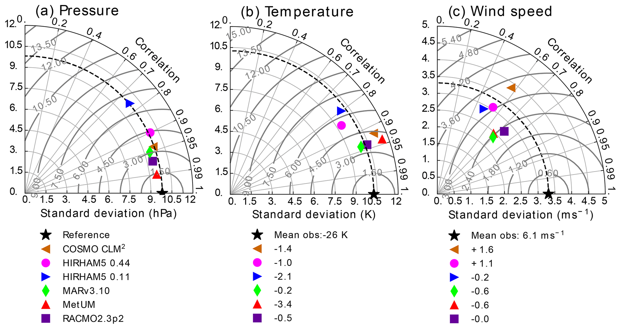
Figure 1Taylor diagrams showing model performance compared to daily observations of surface pressure (a), near-surface temperature (b), and observed wind speeds (c). The horizontal and vertical axes represent the standard deviation; the dashed line in bold shows the standard deviation of the observations. The Taylor plot also shows the correlation which is measured by the angle with the x axis. Finally, the CRMSE is represented by the curved lines in light grey. The units of standard deviation, CRMSE, mean bias, and mean of the observations are the same (hPa for surface pressure, K for near-surface temperature, and m s−1 for wind speed).
Figure 1 analysis shows that, depending on the variable, all the models perform reasonably well though with some variation. With respect to surface pressure, the majority of models are similarly skilful, with the exception of HIRHAM5 0.11∘, which has the lowest correlation and highest bias, although the model is still close to the pattern of the standard deviation. The other models have quite a high degree of nudging, including upper-atmosphere pressure fields within the domain, so it is not so surprising to see the good performance here as the nudging forces the models to be closer to the observed pressure. Without nudging, the large domain size in Antarctica means that synoptic-scale systems have more degrees of freedom to evolve away from the observed quantities. This is likely to be a particular problem for higher-resolution models, where there are more grid points between the boundary and a given station compared to a lower-resolution model with fewer grid points. Our results show that the high-resolution (0.11∘) version of HIRHAM5, which has many more grid cells than the low-resolution (0.44∘) version, has a higher divergence due to internal variability. MetUM is not nudged by surface relaxation but is run in daily reinitialization mode, and while this probably also helps to keep surface pressure close to observed, it is also likely that the large number of atmospheric levels in MetUM also improves modelled surface pressures. The near-surface temperatures in Fig. 1 show that, although overall the models perform well (Pearson correlation of 0.85 and higher), on average all the models are too cold, and only MARv3.10 and RACMO2.3p2 have a bias of less than 1 K (respectively −0.16 and −0.51 K), with MetUM having the highest bias (−3.44 K). As with the surface pressure analysis, the HIRHAM5 high-resolution simulations have a relatively lower correlation coefficient (0.85 compared to above 0.9 for the other simulations), and this may well be again the consequence of the un-nudged simulations. However, biases in cloud cover and long-wave radiation reaching the surface are likely the main explanation for divergence from observations and should be investigated for all RCMs run for Antarctica as shown by van Wessem et al. (2014). In their study, significant improvements in the RACMO2.3p2 model were obtained by adjustments to the cloud microphysics. Furthermore, the lack of detailed subsurface snowpack schemes including processes such as refreezing (and subsequent latent heat release) and densification also likely has an impact on the near-surface and subsurface temperature bias in HIRHAM5 and MetUM (see also Fig. 2).
Figure 1 shows that all of the models perform less well for wind speeds than for temperature or pressure observations. The wind speed plot shows that all models have higher CRMSE, higher standard deviation, and lower correlation values when compared with observations. Even so, the RACMO2.3p2, MetUM, and MARv3.10 still show a correlation above 0.9 with observations, suggesting that the nudging schemes in these models are effective in helping to reproduce observed wind speeds. There are also likely to be large uncertainties in the observations, especially at unattended stations, where burial by snow, changes in orientation, and sensor breakdown are more likely. However, the effects of different resolution and differences in turbulent schemes between the models may also be important. In particular, the extremely stable boundary layer over most of Antarctica is hard to represent in models, particularly at lower resolutions (Zentek and Heinemann, 2020). The models appear to fall into two groups on the Taylor diagram: MARv3.10, MetUM, and RACMO2.3p2 on the one hand and the two HIRHAM5 runs and COSMO-CLM2 on the other hand. In the case of COSMO-CLM2 wind speeds are output at 20 m and then interpolated to 10 m using Monin–Obukhov theory (Souverijns et al., 2019), which may not be sufficient to properly represent near-surface winds and associated interactions. The HIRHAM5 results may again be biased due to the lack of nudging within the domain. However, it is worth pointing out that HIRHAM5 correctly represents the mean spatial variability (both runs are the closest to the dashed line indicating the standard deviation) and, in the case of the high-resolution run, has a very low bias in the mean observed wind speed.
3.2 Comparison with 10 m snow temperature observations
Figure 2 shows the modelled surface temperature of the RCMs as a function of 64 measurements of temperature at 10 m depth as also used by Van Wessem et al. (2014). The majority of the AIS has negligible snowmelt, and in these regions the 10 m snow temperature is representative of the long-term average annual surface temperature. This comparison, therefore, is a robust assessment of the climatological surface signal calculated by the models also because the observations are evenly scattered across the continent and represent most climatic regions. All models capture the wide range of surface temperatures from ≈218 to 260 K. HIRHAM5 0.44∘ consistently underestimates temperature for most locations, a bias that closely resembles RACMO2.1 in Van Wessem et al. (2014) and which the authors concluded was predominantly related to biases in the downwelling long-wave radiation. The other models overestimate temperature in the higher-elevation, colder locations while underestimating temperature at lower elevations in the coastal regions. For the colder regions below ≈240 K, these biases are most likely related to discrepancies in cloud cover, likely snowfall, affecting downwelling longwave radiation and surface albedo. Some of the Antarctic models have been tuned to improve the dry and cold biases in the interior that were persistent in earlier model versions (see RACMO2.1P; Van Wessem et al., 2014; van Wessem et al., 2018) but now overestimate temperature slightly instead. While subsequent model updates have led to significant improvements in simulated SMB, this has come at the expense of surface temperature due to excessive increases in downwelling radiative fluxes that accompany increases in snowfall.
For the lower-elevation, mostly coastal regions, most models have a cold bias. This bias is likely related to the effects of surface meltwater percolating into the firn and refreezing within, raising deeper snow temperature, implying modelled surface temperature is not a good metric for observed 10 m snow temperatures in the percolation zone. A more accurate comparison would therefore be to directly compare 10 m snow temperatures from the models with the observations. However, not all models calculate snow temperatures, and given the scope of this paper, we only intercompare the surface temperature. Here, Fig. 2 illustrates a consistent intermodel scatter, with mainly the models that do not include a sophisticated snow model outside of this range. This points to a significant potential source of improvements for modelled SMB in the future.
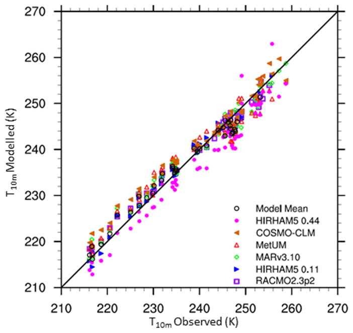
Figure 2Modelled surface temperature as a function of observed 10 m snow temperature (Van Wessem et al., 2014). Observations not fully located on the model ice mask are excluded.
3.3 Comparison with observed SMB
Evaluating SMB is hindered by poor observations across the cryosphere, particularly in Antarctica, where remoteness and extreme weather conditions add to the challenge of observing SMB. Our analysis uses a large dataset of observations, but there are large areas significantly undersampled (see, for example, Fig. A2). We therefore separate the comparison of modelled and observed SMB into elevation bins in Fig. 3 in order to make the results clearer. Note that Fig. 3 is plotted on logarithmic axes because the distribution of both the observed and simulated SMB is not Gaussian. As linear regression is strongly influenced by the extreme values, which skew r2 errors in both modelled and observed SMB for the largest values, but is only weakly influenced by the errors in the smallest absolute values, a logarithmic plot better displays how well models reproduce SMB in both high- and low-SMB regions. It is also important to note that for the scatter plots by elevation class, if an observation or one of the models had a negative value, the observation and modelled values were removed from the analysis using logarithmic values for the scatter plots by elevation class (hereafter, rlog is the correlation computed on the logarithm of SMB values) but are retained in the analysis using the original populations. We show detailed statistics for the SMB comparison in Table 2. In order to show the large scatter in the observations and the models clearly, we also plot all modelled SMB values against observed SMB values in Fig. 4. We show individual model comparisons in the Appendix to save space here (Figs. A3, A4, A5, A6, A7, A8).
Apart from COSMO-CLM2 and HIRHAM5 0.11∘, the RCMs show similar root mean square error (RMSE) and r2 values when compared over the full dataset, but breaking them down by elevation class or locally by regions as in Fig. 4 shows a more complex story. In general, all models, with the possible exception of MARv3.10, underestimate SMB at the ice shelf observation locations as well as in the low-elevation coastal regions of Antarctica (see also statistics in Table 2a and b and Fig. 3). The highest mean bias, lowest RMSE, and lowest r values in particular are given in the COSMO-CLM2 and HIRHAM5 0.11∘ models at the lowest elevations. However, while all the other RCMs underestimate SMB, especially over the Ross Ice Shelf, MARv3.10 overestimates it, probably related to a poorer representation of the surface climate by the model over this ice shelf. There are indications in Fig. 4 that both HIRHAM simulations overestimate SMB on the Ronne Ice Shelf, but we lack observations to be able to test this properly.
The blowing-snow module included in RACMO2.3p2 may explain the lower bias and RMSE in this model at elevations between sea level and 1200 m and especially 1200 and 2200 m (we show all statistics in detail in Table 2b and c) compared to the other models. A previous comparison shows higher sublimation in RACMO2.3p2 than in MARv3.10 (Agosta et al., 2019), notably at the elevations where katabatic winds are strong due to the slope of the ice sheet and where the atmosphere is not too cold, enabling large amounts of sublimation from blowing snow particles. COSMO-CLM2 and HIRHAM5 0.44∘ have the highest RMSE, while HIRHAM5 0.11, MARv3.10, and MetUM have similar statistics at this elevation. For the highest elevations (above 2200 m), all the model RMSE scores are relatively low and similar to each other, except HIRHAM5 0.44∘ (and to a lesser extent MARv3.10) between 2800 and 3400 m (Table 2e). However, the less extensively optimized models (HIRHAM5 at both resolutions and MetUM) are both too dry over the high plateau of the AIS.
If we look at all the elevation ranges, no model is systematically in the top three for every range, but RACMO2.3p2 has the best comparison with all the observations, closely followed by MetUM, with MARv3.10 and HIRHAM5 0.44∘ performing almost equally. It is worth emphasizing though that as Fig. 4 shows, the observations in this elevation class are also very noisy, and the poor relative performance of the models may result as much from unrepresentative and sparse repeat observations as it does from missing or poorly resolved processes in models. Analysis of these results indicates not only areas where models need to be improved but also areas where more observations to test models are desirable, notably between 1200 and 2200, where the mean biases of the models used in this study display large discrepancies (Table 2c). It is also likely that there are compensating errors within each model that hide the true performance. For example, the mean bias between the two different HIRHAM runs has opposite signs in the 1200–2800 m range, likely reflecting the difference in model resolution. Orographic precipitation is very sensitive to slope effects, and the presence of steep topography is very different between the two resolutions, affecting where precipitation falls across the continent. The wide scatter in modelled SMB in the 2200–2800 m elevation range is therefore also likely to reflect in part the resolution of the different models and how well they capture orography and the consequent precipitation. Studies by, for example, Hermann et al. (2018) and Schmidt et al. (2017) show that hydrostatic models like HIRHAM5 and RACMO2.3 typically overestimate precipitation on the upslope and have a dry bias downwind of initial steep topography; this pattern seems to some extent to be repeated in Antarctica in Figs. 3 and 4. Comparing the observations used in this analysis with the RCM ensemble, modelled SMB in Fig. 6 also highlights that the largest differences between models and compared with the ensemble mean are mostly in regions with very few or no observations. These are also regions where precipitation is typically high, making it difficult to assess the ability of models to truly simulate the SMB of Antarctica. Our analysis therefore also helps to identify areas where increased observations will be most useful to help assess and improve model processes.
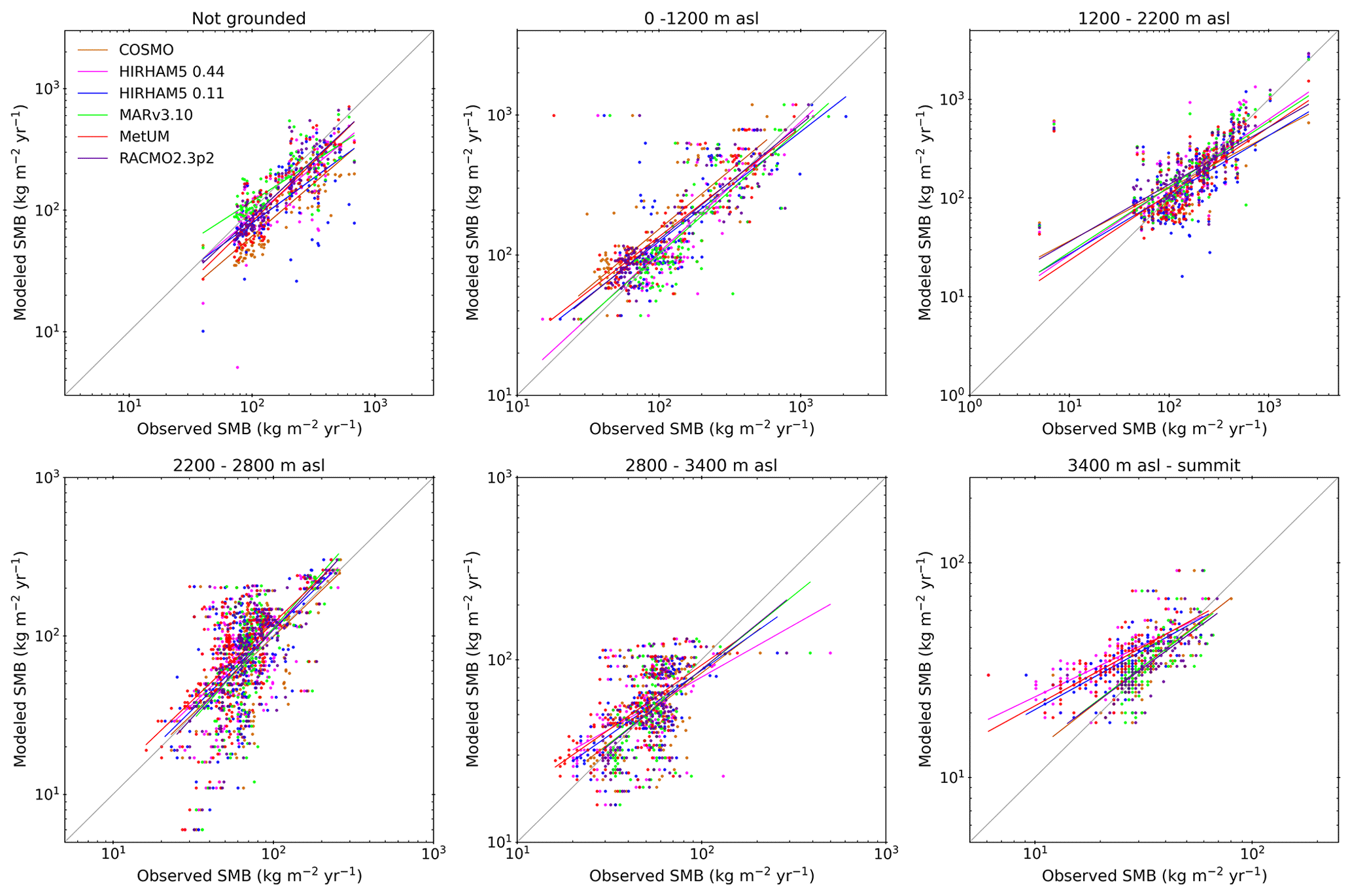
Figure 3Comparison between modelled SMB and observed SMB in a gridded dataset. Trend lines and points are plotted for each model in a different colour. Note different x and y axes for different elevation bins. The figures are plotted on logarithmic axes because the datasets do not have Gaussian distributions, and this better represents the relative error in both high- and low-SMB regions than linear axes.
Mean bias and RMSE for each model by elevation bin is summed up in the Appendix in Figs. A3 to A9. However as Fig. 4 also shows, this is not a straightforward comparison either due to the large areas with only few observations.
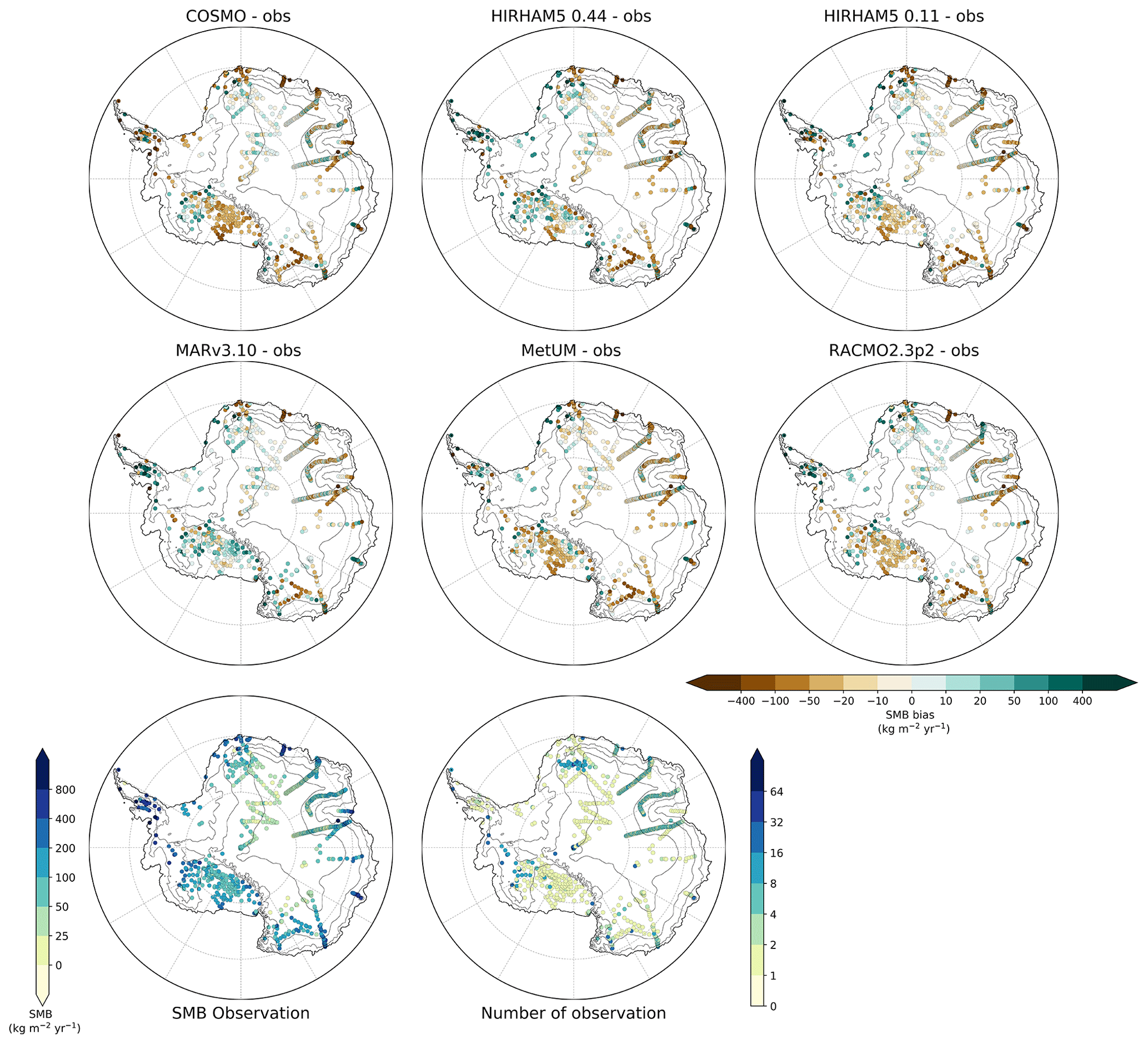
Figure 4Observed SMB values and the number of observations at each point. The model plots show the difference between observed and modelled SMB for COSMO-CLM2, HIRHAM5 0.44∘, HIRHAM5 0.11∘, MARv3.10, MetUM, and RACMO2.3p2.
Table 2Comparison of the modelled SMB to the SMB observations over the ice shelves (a), by elevation bins (b–f), and over the whole AIS (g). Unit of mean bias (MB), root mean square error (RMSE), and mean of the observation is kg m−2 yr−2. N denotes the number of comparison used for each bin, while L represents the number of comparisons that used the log distribution.

3.4 Assessing the surface mass balance of Antarctica
Bearing in mind the results presented in the preceding section evaluating the RCMs, we show here the range of best estimates for Antarctic SMB based on RCMs. Figure 5 shows the modelled specific surface mass balance (SSMB); this is defined as the SMB integrated over the whole basin and divided by the area. We use the 19 drainage basins defined in Shepherd et al. (2020) for the full 9 climate simulations as well as the ensemble mean and standard deviation in order to better compare the more recent estimates in this study with older modelled results. Figure 5 also lists the total integrated SMB of the basin in units of gigatonnes (shown by the numbers in a box in each basin). All models simulate a comparable SSMB for the East Antarctic ice sheet (EAIS), with values between 100 and 400 mm yr−1. Due to the moist coastal climates over the ice shelves, SSMB values here reach values as high as 1000 mm yr−1. The main intermodel differences are found over the West Antarctic ice sheet (WAIS) and the Antarctic Peninsula (AP) and are most likely related to differences in horizontal resolution and, therefore, orographic precipitation. The higher-resolution models (RACMO2.3p2, HIRHAM5 0.11∘, and MARv3.10) generate the highest SSMB values over the AP and WAIS basins, up to 2000 mm yr−1. The other models have considerably lower SSMB, especially over the adjacent ice shelves. COSMO-CLM2 is drier than the ensemble mean and all other models in all basins, with the exception of the Queen Mary Land basin in the EAIS, where HIRHAM5 0.11∘ is slightly drier, and the interior of the EAIS, where MARv3.10 is slightly drier. The two areas with the largest ensemble mean deviation are the western-peninsula basin but also the interior of the EAIS bordering the Transantarctic Mountains and including the South Pole. In this region the MARv3.10 model has the highest SMB (196 Gt), but MetUM has the lowest (77 Gt). Figure 5 also shows some of the striking features in the pattern of SMB present in all the models where the magnitude differs; for example, all models have a steep gradient in the SMB over the Antarctic Peninsula, but this is much more pronounced in HIRHAM5 0.11∘ than in HIRHAM5 0.44∘, demonstrating the importance of resolution in this region. MetUM and COSMO-CLM2 also show the same pattern but with considerably lower absolute values, particularly on the western side, than the other models. These differences in modelled SMB on the basin scale may have a considerable impact on dynamic ice sheet models used to determine the evolution of the AIS and are consequently important to take into account when selecting SMB to force ice dynamics models. Looking at the total surface mass budget including ice shelves for the period 1980 to 2010 (numbers in the caption and summarized in Table 3) generated by the models, the HIRHAM5 0.44∘ simulation is the wettest model (2752 Gt yr−1; 2328 Gt excluding ice shelves), while COSMO-CLM2 is the driest (2031 Gt yr−1; 1751 Gt excluding ice shelves). The other simulations are all closer to each other and are within an SMB range of ±200 Gt yr−1, while the two dedicated polar models (RACMO2.3p2 and MARv3.10) have only a small difference of 83 Gt yr−1 on average, corresponding to around 3 % of the total budget. These two models have been evaluated and optimized for Antarctica the most intensely of all the models (van Wessem et al., 2018; Agosta et al., 2019). We also include MAR3.6 and RACMO2.1 in this figure to give context to earlier studies. The two closest models overall are in fact HIRHAM5 0.11∘ and MARv3.10, which differ by only 26 Gt overall, with much of the difference accounted for by the SMB of the ice shelves.
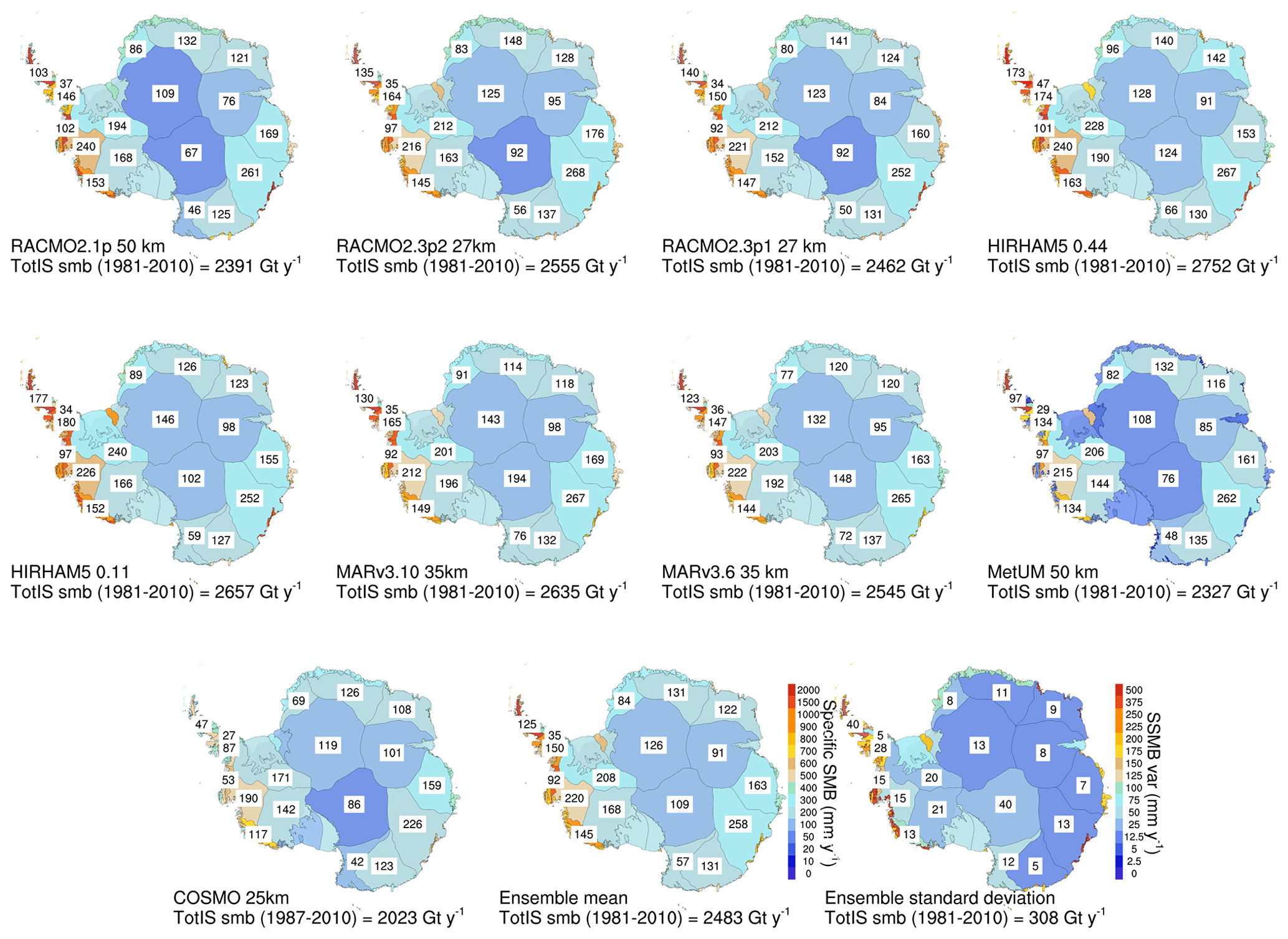
Figure 5Integrated SMB and specific SMB (SSMB) for the nine models included in this study (RACMO2.1, RACMO2.3p2, RACMO2.3p1, HIRHAM5 50 km, HIRHAM5 12.5 km, MARv3.10, MARv3.6, MetUM, and COSMO-CLM2) as well as the ensemble mean and standard deviation shown. Colours denote the SSMB in millimetres of water equivalent per year for all grounded ice sheet basins as well as the ice shelves these drain into, defined in Shepherd et al. (2019). The numbers included in the basins denote the basin-integrated SMB in Gt yr−1 for the grounded ice sheet for the period 1980 to 2010 with the exception of COSMO-CLM2, where the time series starts in 1987. Finally, the total integrated number for the grounded ice sheet including ice shelves is shown in the figure label.
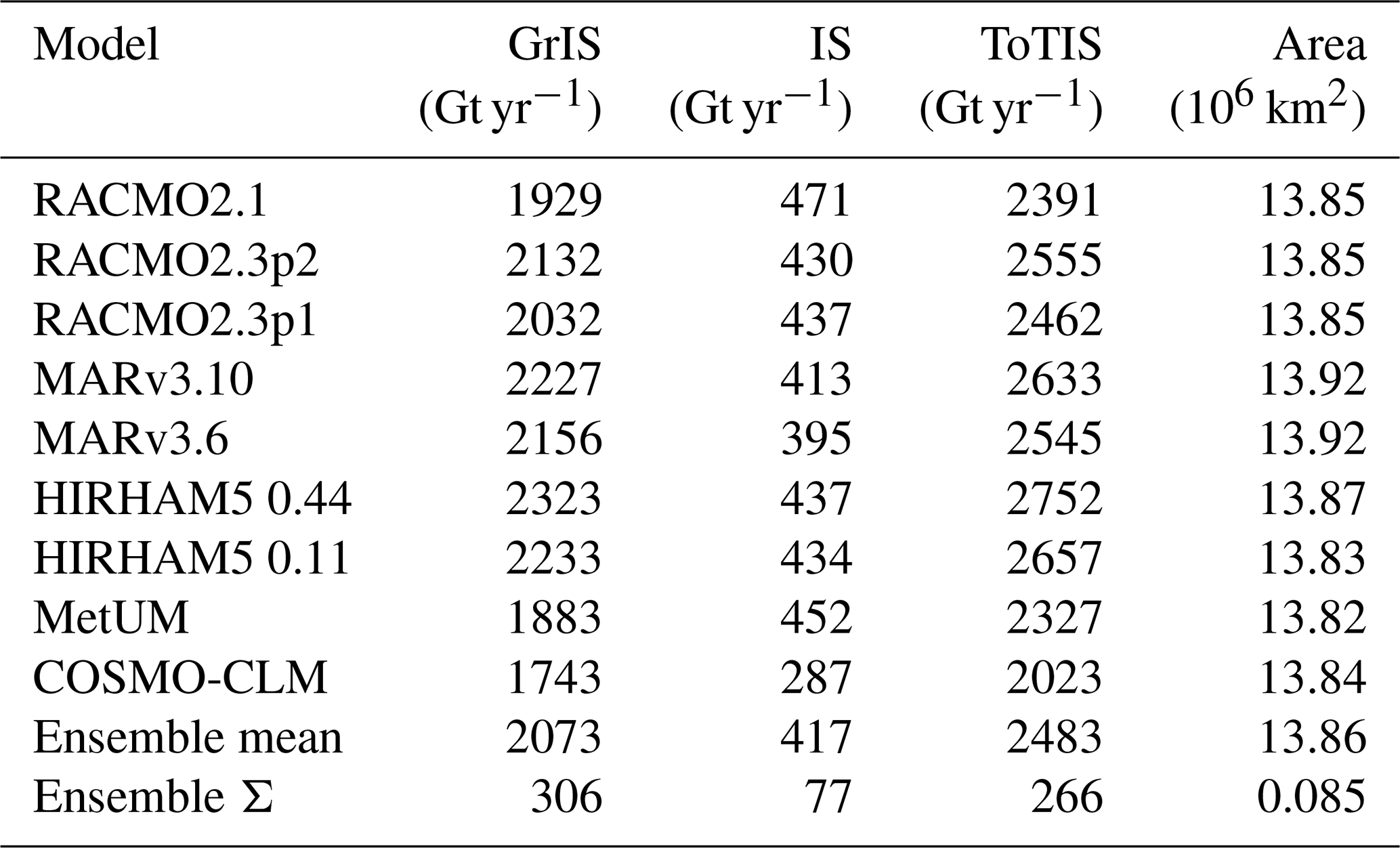
Table 3Integrated mean annual SMB for the six models used in this study for the period 1980 to 2010 except for COSMO-CLM2, where the period was 1987 to 2010. Three older model versions, ensemble mean, and standard deviation as shown in Fig. 5. All calculations done on the original grid of the individual models using a common set of drainage basins and ice mask defined by IMBIE2 (IMBIE2 is the second assessment by the ice mass budget intercomparison exercise, published by Shepherd et al., 2020). The ensemble mean was calculated by transforming all models to the RACMO2.3p2 grid. GrIS denotes grounded ice sheet, IS denotes ice shelf, and ToTIS denotes the full AIS including ice shelves.
As the basin-scale SMB values differ quite substantially between models, in Fig. 6 we plot the mean annual SMB from the ensemble mean and the anomaly to that for each of the different models. The ensemble mean is calculated on a common grid, but the model anomalies are calculated from it on their own grids, which more clearly shows the effects of the different resolutions on the SMB. The figure shows quite substantial agreement between models over large areas of Antarctica but also some considerable local variability. Features such as the Transantarctic Mountains and the rugged coastal topography in West Antarctica, both of which substantially influence local weather patterns, are picked out in the spatial pattern of the SMB. These features are more clearly delineated in the higher-resolution runs. However, the ensemble mean can also hide large disagreements between the models. For example, there is an interesting asymmetry in the model results for the region of the Queen Maud Mountains and Queen Elizabeth ranges of the Transantarctic Mountains. The MAR model and to a lesser extent the HIRHAM5 0.44∘ model show rather different patterns in SMB compared to the other models, with higher SMB south of the range and lower-than-ensemble mean values north of the range. The other models show the reverse, with values lower than the mean south of the range and higher to the north. A similar but less clear pattern is also seen along the Ross and Amundsen Sea coastal sectors. The coastal margin of the whole continent in general shows a blotchy pattern in the SMB anomaly plots that reflects rugged topography. In these regions the resolution of the model determines the location of orographic precipitation. Analysis of similar SMB simulations in Greenland with the HIRHAM, MAR, and RACMO models (Hermann et al., 2018; Schmidt et al., 2017) suggests that in these types of locations HIRHAM and RACMO overestimate precipitation at lower elevations in steep terrain, whereas MAR tends to have a wet bias at a slightly higher elevation, where the other two models are drier. Agosta et al. (2019) related this different pattern of biases in MAR to the advection of precipitation in the model's prognostic precipitation scheme. Understanding these biases is crucial to understanding and interpreting modelled SMB, and comparing Fig. 6 with Fig. 4 it is clear that the locations where there is the highest disagreement between models are also the regions with the poorest systematic observational coverage of SMB, especially in coastal regions and in West Antarctica.
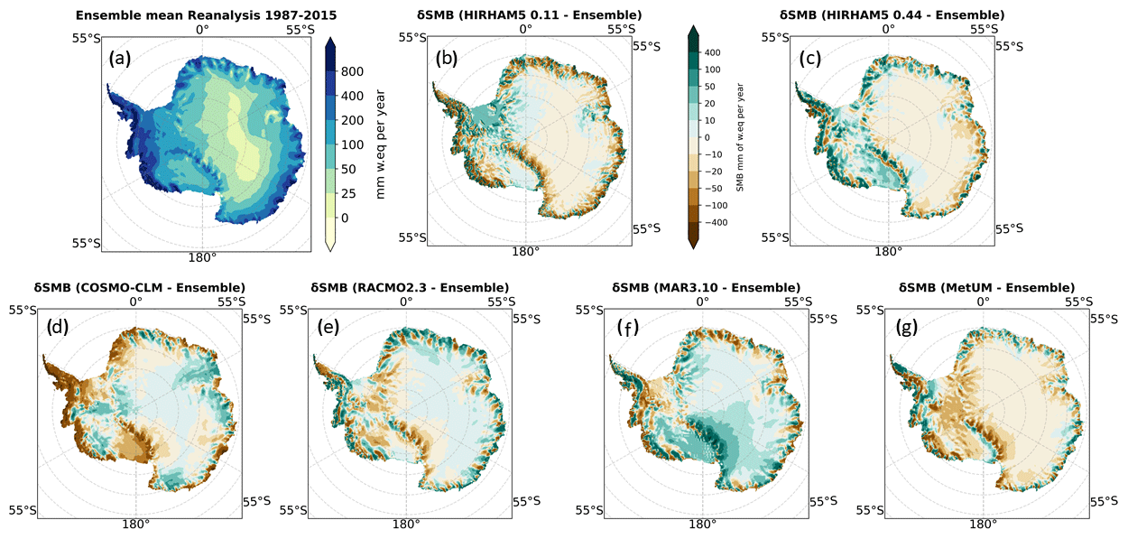
Figure 6Panel (a) shows the SMB ensemble mean for the common period on the common mask. Panels (b)–(g) show the difference between each model and the ensemble mean.
SMB varies not only spatially but also temporally, and average annual SMB values hide large interannual variability of around 4 % in SMB as depicted in Fig. 7. The spread in the range of estimates of SMB is, however, consistent from year to year. The integrated continental SMB calculated over the common mask has a spread of more that 550 Gt between the highest and lowest estimate on average (see also Table 4), but all the models show similar annual- and decadal-scale variability. This implies that the driving model, in this case ERA-Interim, is the most important source of SMB variability but that the individual models are important when considering both the absolute number and the local spatial variability.
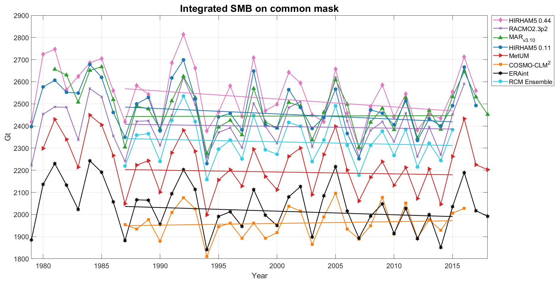
Figure 7Annually resolved SMB integrated over the common ice mask for the different RCMs in the period 1979–2018. All RCMs are driven by ERA-Interim, and except for MARv3.10 and RACMO2.3p2, SMB is calculated according to Eq. (1). The ensemble is a mean calculated from all six RCMs in the period 1987–2015, where there are data from all the models. All trend lines are calculated for the period 1987–2015.
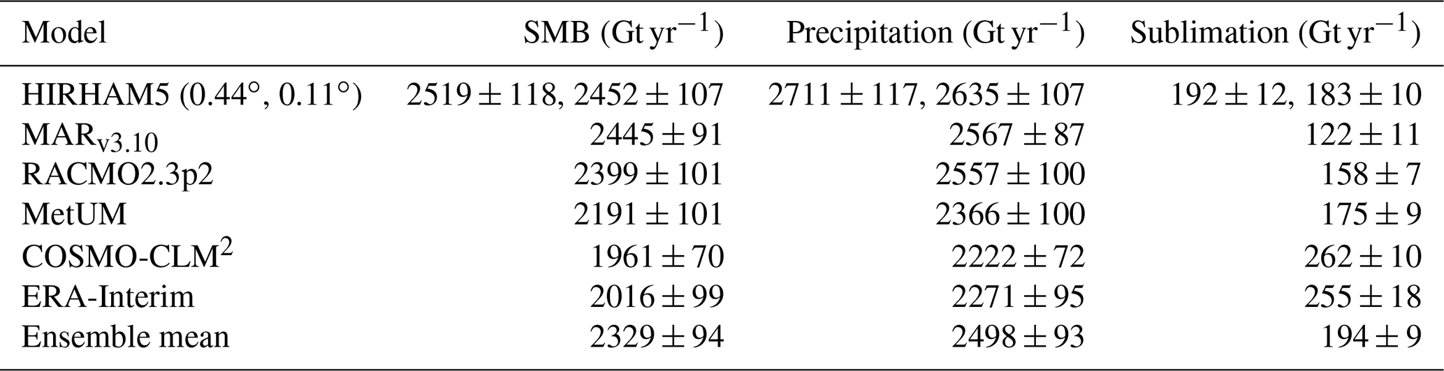
We calculate the mean annual SMB and components across the continent including ice shelves, as given in Table 4, over the period 1987 to 2015, for which outputs are available for all the models. Note that this is calculated over a common ice mask and a common simulation period and using the simple SMB calculation given in Eq. (1), and results are therefore slightly different to those already published for different models or shown in Fig. 5 or Table 3. The simple SMB is used to compare the models more fairly against each other and with the ERA-Interim-derived SMB in Figs. 7 and 6. In this time series HIRHAM5 0.11∘ and MARv3.10 are the closest two models to each other in integrated SMB. RACMO2.3p2 is closest to the ensemble mean, but COSMO-CLM2 is closest to the driving ERA-Interim modelled values. The trend lines are very sensitive to starting and ending years and in some cases change sign if a longer period is chosen, but as we have only a short common period we have chosen to calculate the trend over the common period. For this chosen period, COSMO-CLM2 and MARv3.10 show a slightly increasing trend in SMB, whereas the rest show a slightly declining trend in SMB, although the trend in RACMO2.3 and MetUM is almost flat. The ERA-Interim trend over the period declines slightly more than the MetUM trend, which is otherwise extremely close. The different trends from the models and in particular the sensitivity to different start and end points do not give us confidence to ascribe a statistically significant trend to Antarctic SMB over the whole continent. We note though that all models show a declining trend in the 1990s and early 2000s but with a recent increase in SMB since 2014. The early part of the record appears to have higher variability, but this may be related to changes in data assimilation in the driving reanalysis (Dee et al., 2011).
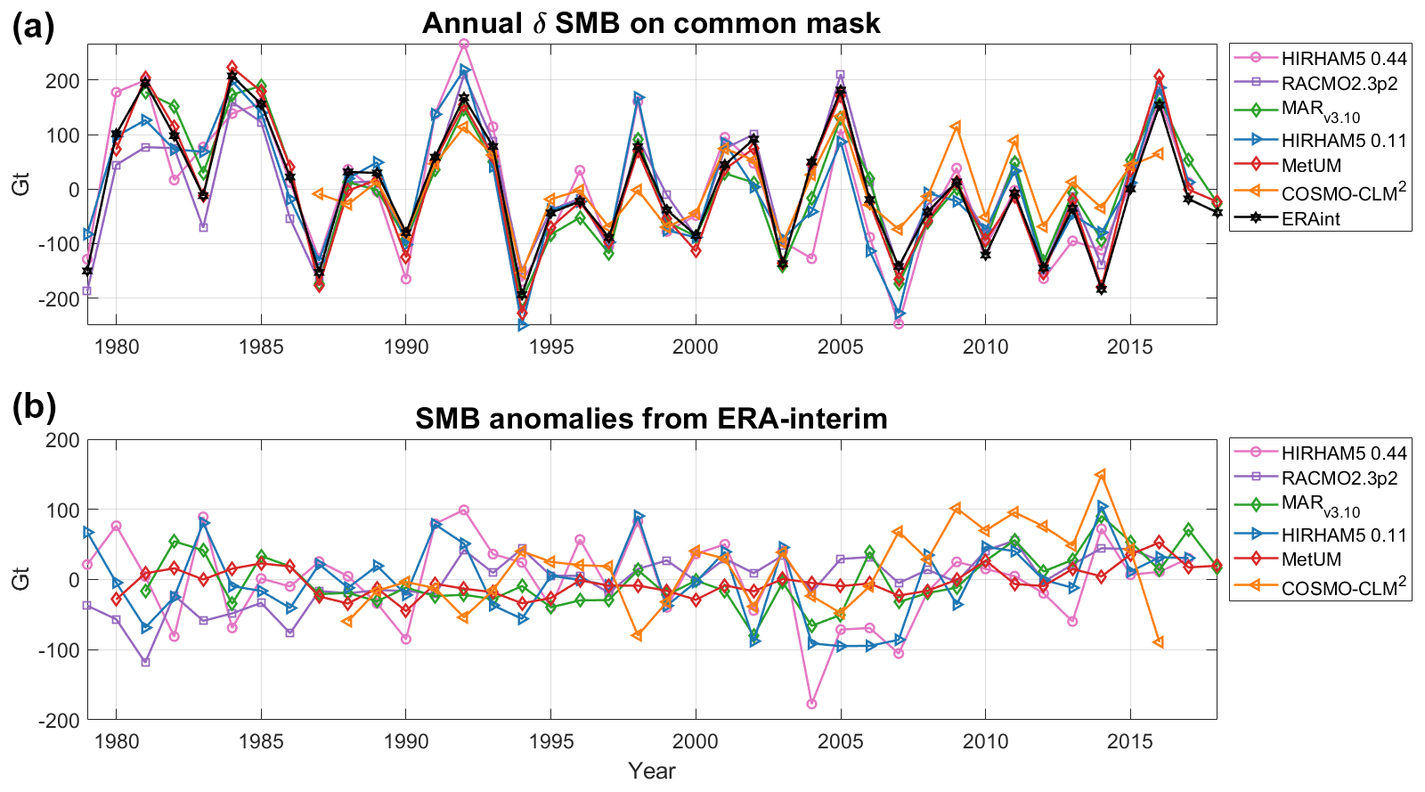
Figure 8Panel (a) shows the annual variability in surface mass balance over the common mask for each of the different RCMs in the period 1979–2018. It is calculated by subtracting the respective model mean from each RCM's SMB time series. Panel (b) displays how modelled SMB from each RCM deviates from the ERA-Interim SMB.
Figure 8 emphasizes the large variability in SMB on an annual to decadal scale by plotting the variation from the mean for each model and the variation from ERA-Interim for each model. We show that while all the models have more or less the same anomaly when compared to their own mean, the sign of the anomaly compared to the ERA-Interim value can be different. Since the most highly constrained models show the lowest anomaly compared to ERA-Interim, we suggest that most of the variation is related to internal variability (weather) within the domain. Both HIRHAM5 0.11∘ and 0.44∘ show the highest values of variability, probably due to the unconstrained nature of the runs, but in different years, different models show higher variability than the others. The lower panel in Fig. 8 demonstrates that MetUM is by far the closest to the driving model, with much less variability than the others (likely due to its frequent reinitialization). HIRHAM5 again shows the highest difference compared to the driving model, but from year to year the model showing maximum difference varies, and there appears to be no systematic pattern as to whether or not modelled SMB is higher or lower than the ERA-Interim reanalysis when quantified on the common mask and over the whole of Antarctica. The implication is that while the driving model controls broad-scale pattern of SMB, the downscaling model adds its own weather variability to the broad-scale pattern. The variability, or weather noise, is unsurprisingly largest in un-nudged models. The effect of this noise on ice sheet dynamics may be small overall, but, as for example, Mikkelsen et al. (2018) show, small stochastic variations in SMB can have a non-negligible impact on ice sheet dynamics.
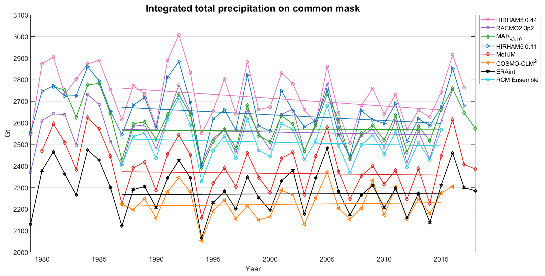
Figure 9Annually resolved precipitation integrated over the common mask for the different RCMs in the period 1979–2018. All RCMs use ERA-Interim. The ensemble is a mean calculated from all five RCMs in the period 1987–2015, where all models have data.
Since SMB is made up of accumulation and ablation components, and in Antarctica precipitation is the dominant term, Fig. 9 shows the precipitation component only over the common mask for the different models and ERA-Interim. There is a very similar pattern to that in Fig. 7, but compensating effects from sublimation, which is higher in HIRHAM than in MAR, explain the bigger offset between HIRHAM5 0.11∘ and MARv3.10. MAR is closer to RACMO2.3 in terms of precipitation, separated by only 10 Gt. The mean values for the SMB components of precipitation, evaporation, and sublimation as well as SMB for the common period 1987–2015 over the common ice mask are also displayed in Table 4. These values confirm that the very much higher precipitation in both HIRHAM5 runs compared to the other models is to some extent compensated for by higher values of sublimation. Precipitation in HIRHAM5 0.44∘ is 80 Gt higher than that in the 0.11∘ simulation, which in turn is 68 Gt higher than the next wettest model, MARv3.10, but precipitation in the RACMO2.3 model is only 10 Gt lower than in MAR. On the other hand, sublimation in HIRHAM5 is higher (192 and 183 Gt in the 0.44 and 0.11∘ runs, respectively) than in MARv3.10 (122 Gt), RACMO2.3p2 (158 Gt), and MetUM (175 Gt), but COSMO-CLM and ERA-Interim both have higher values than HIRHAM (262 and 255 Gt, respectively). Although the RACMO2.3p2 model includes sublimation from ventilated snow, the sublimation rates are still lower than all models except MARv3.10. MetUM, which performs similarly to RACMO2.3 when compared with SMB observations, has lower precipitation and higher sublimation rates than RACMO2.3, however, suggesting that ventilation of drifting snow alone does not explain the higher sublimation rates. MARv3.10 has the lowest sublimation rates of all and COSMO-CLM2 the highest. Our results suggest that the dry bias in COSMO-CLM2 is a result in part of the lower precipitation values, which are very close to those of the driving ERA-Interim model but also a consequence of the much higher sublimation values. This dry bias is mostly confined to the coastal regions and peninsula and is identified and discussed in Souverijns et al. (2019). The RACMO2.3 model is closest to the ensemble mean annual precipitation, but as the MARv3.10 model mean values are only different to RACMO2.3 by 10 Gt, in some years shown in Fig. 9 it is actually even closer to the ensemble mean than RACMO2.3 is.
Table 4Mean annual SMB and components on common mask for each model averaged over the 1987–2015 period, where all the models overlap. Standard deviations are also shown. SMB is calculated using the simple Eq. (1) to enable a fair comparison.
4.1 The surface mass budget of Antarctica
The range of models in this intercomparison study allows us to not only estimate the likely range of SMB over Antarctica but also to identify sources of disagreement and bias within and between models. Accounting for differences in ice mask, the ensemble mean annual SMB integrated over the whole of Antarctica between 1987 and 2018 is 2329 ± 94 Gt yr−1. The RACMO2.3p2 model has a value closest to the ensemble mean, with the high-resolution HIRHAM5 model 190 Gt over this number and the COSMO-CLM2 model 368 Gt below. The HIRHAM5 0.11∘ and MARv3.10 numbers are almost exactly the same, at 2452 and 2445 Gt yr−1, respectively, around 150 Gt above the mean. MetUM and COSMO-CLM2 are much lower, at about 138 and 368 Gt below the mean, respectively. Given that the models perform fairly similarly when evaluated against SMB observations, we here give all models equal weight, although we suspect that there is a dry bias in COSMO-CLM2 and a wet bias in HIRHAM5 0.44∘. With an identical forcing from ERA-Interim, the present-day estimate of the surface mass budget of Antarctica ranges from 2519 to 1961 Gt yr−1, a 558 Gt range that alone is equivalent to around 1.5 mm of global mean sea level rise. Narrowing this range for the purposes of estimating sea level change at present and in the future is an important task, and for this reason we have evaluated the models against observations in Antarctica (see below).
We can compare our results for the total mass budget of Antarctica with those produced by the IMBIE2 study (Shepherd et al., 2020). In Fig. 10 we show the SMB discharge for two different datasets, where the IMBIE2-reconciled (Shepherd et al., 2020) estimate of mean annual discharge is 2103 ± 56 Gt yr−1, and the discharge of 2247 ±140 Gt yr−1 estimated by Rignot et al. (2019) for the same period is subtracted from SMB calculated from each model. We use the simple SMB calculation in Eq. (1) for the period 1992 to 2017 over the grounded ice sheet only. The Rignot et al. (2019) dataset has a wider uncertainty range than the Shepherd et al. (2020) estimate and a larger discharge that gives a lower total mass budget overall, but in all cases the two overlap within the uncertainty ranges. Note that the RACMO2.3p2 model was used to produce both the IMBIE2 and Rignot et al. (2019) estimates, and it is thus not a truly independent comparison. The earlier MARv3.6 model was also included in the Shepherd et al. (2020) study.
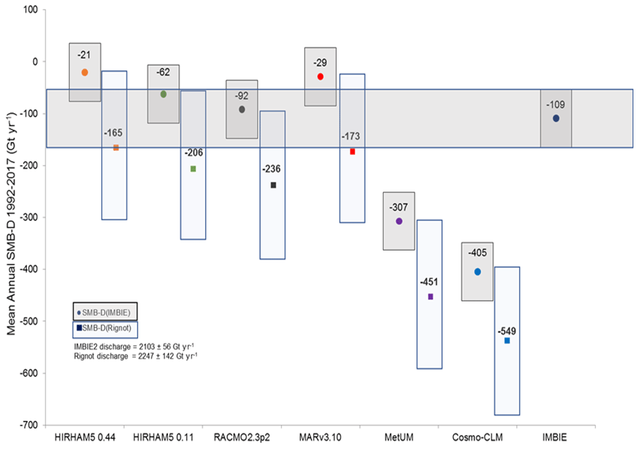
Figure 10Modelled SMB minus discharge calculated from IMBIE2 results (Shepherd et al., 2020) (filled circles indicate mean; light-grey box indicates IMBIE2 uncertainty range of ±56 Gt yr−1) and Rignot et al. (2019) (mean showed in filled square; uncertainty range of 142 Gt yr−1 shown by narrow shaded blue box). The range for the Rignot discharge is taken from Table 1 in Rignot et al. (2019). We assume that the same uncertainty range for the period 2009 to 2017 is applicable over the longer 1992–2017 period. The total mass budget estimated by IMBIE2 is also shown by the horizontal shaded dark-grey box for ease of comparison. Numbers are mean annual SMB-D for the 1992–2017 IMBIE period for each model.
When taking into account the published uncertainties in the observational mass budget estimates of discharge, only the COSMO-CLM2 and MetUM estimates are completely outside the range defined by the IMBIE study (109 ± 56 Gt yr−1) for the total mass budget of Antarctica. However, as the statistics in Fig. 1 show, both models perform well compared to the weather station observations, particularly MetUM, and both have higher correlations and lower biases than the two HIRHAM simulations) for pressure and temperature. Comparison with the SMB observations shows that while COSMO-CLM2 has a large dry bias (of ∼40 %) over ice shelves and at lower elevations, at higher elevations the mean bias is close to zero for the COSMO-CLM2 model and in fact much lower than the other models in the 2800–3400 m elevation range (see Fig. A9). MetUM on the other hand has a middle-of-the-range mean bias at low elevations compared to other models but a much higher (−25 % to −30 %) mean bias as shown in Fig. A9 at the upper elevations. The combination of these results, bearing in mind also the undersampling in the dataset, thus indicates either that some of the components of SMB are poorly captured by the models or that there are compensating errors in the modelled SMB components and/or their spatial variability. Most likely a combination of factors is responsible for the wide variation in integrated SMB estimates. This means that there are large uncertainties in both observations and the biases in models that we discuss in this paper that complicate assessing the contribution to sea level rise from Antarctica from SMB processes.
Unlike previous studies, we detect no obvious strong trend in the modelled SMB in any of the models or in the driving ERA-Interim model. Shorter periods within the time series appear to have quite strong trends. For example, a steady declining trend is apparent through the 1990s and 2000s but appears to reverse after 2014. Our results suggest that strong interannual and decadal variability makes the identification of meaningful trends over periods shorter than multidecadal very difficult. Distinguishing noise from signal will be challenging in the coming decades, and this also emphasizes the importance of long time series of observations. SMB variability is a result of low- and mid-latitude weather variability, but interannual variability is particularly large at the beginning of the ERA-Interim period up to 1990, and we hypothesize this is related to improved data assimilation in the Southern Hemisphere in the period between 1979 and 1989 (Dee et al., 2011). The models disagree on both the magnitude and the sign of the overall trend in the 1987–2018 common period of all models. Figure 8 demonstrates that the external forcing model, in this case ERA-Interim, is extremely important in determining both the total SMB and the year-to-year variability in the SMB trend, even though the absolute values are somewhat dependent on the individual RCM. This is not an unexpected result given that these are all limited-area models forced at the boundaries, but it has important implications for estimates of future projections of SMB in Antarctica. Decadal- and multidecadal-scale climate variability expressed in global climate models will have a strong influence on Antarctica mass budget (including the dynamical components via ocean forcing) that may suppress or enhance the anthropogenic forcing in ways that are difficult to predict given the large internal variability in the system. Long climate simulations with large ensembles will be necessary to define the likely range of internal climate variability, and this poses challenges of computing resources when regional downscaling is required to represent the spatial patterns of SMB over the ice sheet at high resolution.
Even between models with similar values for the integrated SMB, there is substantial spatial variability in the pattern of SMB, as shown by the basin-level breakdown in Fig. 5 and the variation from the ensemble mean in Fig. 6. These together show a nuanced picture. Over most of Antarctica, particularly in the east, the variation between models is rather small; the biggest deviations are largely around the coast. These small areas have a disproportionate influence on the continental integrated SMB values due to high accumulation rates. Basins in West Antarctica, and particularly on the Antarctica peninsula, have very large differences, where, for example, HIRHAM5 0.11∘ shows an average annual SMB of 176 Gt, but COSMO-CLM2 has the lowest estimate of 46 Gt in the same basin. The MAR model, which shows an integrated SMB value similar to HIRHAM5 over the whole continent, gives 130 Gt in the same basin, closer to the RACMO2.3p2 value of 134 Gt, while MetUM is again lower at 96 Gt. Averaging SMB over the whole continent smooths out a good deal of the spatial variability, which in turn is also important for driving ice dynamics. Equally, as some basins especially in West Antarctica have very high precipitation rates, differences between models in relatively small areas here can make a large contribution to the difference in the integrated numbers over the whole continent.
Similarly, relatively small differences in ice masks that are primarily in coastal regions with high accumulation rates can lead to relatively large differences in SMB estimates (see Fig. A1), as Vernon et al. (2013) have also shown in Greenland. Figure A1 in the Appendix compares the ice masks of all the models. We found that, although the variation looks quite small, the grid points affected include some of the highest precipitation points within the domain, and thus small differences can have large effects. This is one of the main differences between the earlier RACMO2.1, with one of the smallest ice masks, and RACMO2.3 for example. Almost all the other models were larger around the entire coastline. The total SMB integrated over the continent is therefore highly sensitive to the size of the common mask. For example, the SMB for HIRHAM5 0.11∘ is computed on its native mask and gives an integrated SMB on average 9.95 % higher compared to the common mask result, even though the native mask is only 2.93 % larger than the common mask. These differences suggest that the CORDEX community should agree on a common protocol to calculate the ice mask to reduce uncertainties in Antarctic SMB. The deviation from ensemble mean SMB shown in Fig. 6 suggests that while over the high plateau of East Antarctica there is little deviation in general, much bigger differences occur between model SMB estimates around the Transantarctic Mountains, where the effect of higher resolution becomes obvious in resolving the topography, but model physics also likely play a role. We see a similar effect in the high-relief topography of West Antarctica. Finally, our results show that between 14 % (COSMO-CLM2) and 19 % (MetUM) of the SMB is accounted for by the ice shelves around Antarctica.
A comparison of the high- and low-resolution HIRHAM5 simulations is interesting here as the models are identical other than resolution. There is a substantial difference in the location of the maximum upslope precipitation as well as the downslope precipitation shadow. We attribute these differences to resolution that allows high-resolution simulations to better represent steep topography. A similar but less marked impact is seen between the earlier RACMO2.1P and newer RACMO2.3p2, though in this case changes in model physics may also be responsible.
4.2 Model evaluation with observations
Evaluating the models against observations is very important for assessing where there are important biases, but evaluation of model performance is significantly hampered by the lack of observations in key regions. Nonetheless, Fig. 1 shows that the models do have skill in simulating surface climate, particularly temperature and pressure. The skill in simulating surface climate does not however translate perfectly to simulating SMB, partly due to the difficulties of modelling and evaluating precipitation. Our analysis shows that, for example, COSMO-CLM2 better simulated surface climate compared to observations than HIRHAM5, but it has a lower skill in SMB. Variables such as temperature and pressure are more easily measured and are assimilated into the reanalysis used to drive the models. RCMs have also been optimized to give good performance compared to these kinds of observations. However, Antarctic SMB is dominated by the precipitation term that is much harder to measure accurately and also has much higher uncertainty in models.
SMB observations themselves are not always very reliable, and sub-grid-scale surface snow processes, such as the build-up of sastrugi, can give substantially different results over short spatial scales (Andersen et al., 2006). Therefore, it is important to break down the data into different regions and elevation classes to see where models have better or weaker performance. We note the scatter in both models and observations within the different elevation bins and that the two polar-optimized models (MAR and RACMO) perform, broadly speaking, better than the others (see also Figs. A3 to A8 in the Appendix), though the differences are rather small in some of the elevation bins and are not always very significant. It is clear that more work needs to be done to understand exactly how SMB varies spatially over the continent in order to better optimize parameterizations. The use of nudging in models does however seem to make it easier to replicate both observed climate and SMB in RCMs. We discuss further below the use of nudging in regional climate simulations.
4.3 Ice sheet SMB processes
Evaluation against observations helps to identify missing and mischaracterized processes within RCMs. Models that have not undergone specific adjustments for Antarctica represent the SMB in Antarctica more poorly than those that have been adjusted in some regions. However, Table 2 shows that introducing new parameterizations is not unambiguously an improvement as in some elevation bands the unmodified models have lower bias and RMSE, as also shown in the Appendix (Fig. A9). Other biases are also evident in this analysis. The driest model, COSMO-CLM2, underestimates SMB close to the coast, a region very relevant for total ice sheet mass balance. This is due to an overestimated sublimation amplified by an underestimated snowfall rate close to the coast. High values for the sublimation originate from an underestimated albedo due to ageing of the snow that occurs too fast in the model (Souverijns et al., 2019). The low values for the snowfall rate are likely related to cloud microphysics, namely a too slow conversion of ice to snow or a too slow deposition of water vapour on the solid hydrometeors. Currently, efforts are ongoing to improve the coastal SMB performance in COSMO-CLM2. The HIRHAM5 climate simulations both appear to have a wet bias, likely again related to the cloud microphysics and precipitation schemes but also probably a result of a diagnostic precipitation scheme commonly used in hydrostatic models. The models typically have a wet bias on the upslope of steep topography and a dry bias on the downslope. The RACMO2.3 model shows a similar, though less pronounced effect that derives also from the IFS physical schemes (Hermann et al., 2018; Schmidt et al., 2017). New prognostic precipitation schemes have been developed for numerical weather prediction models to solve this problem (Forbes et al., 2011), and implementation of a similar prognostic scheme in MAR probably explains the different pattern of SMB in areas with steep topography (Agosta et al., 2019). As RACMO and MAR are the only two models that have a specific subsurface scheme for ice sheets, in this model comparison we have excluded detailed discussion of melt and run-off, and this will likely be the subject of future work. Given the high amount of precipitation over Antarctica, this run-off is still very small in absolute and relative senses, accounting for only 2 Gt of mass loss from the grounded parts of the AIS in RACMO2.3p2 for instance, but as a warming future climate is expected to bring increasing amounts of melt, a more sophisticated treatment that includes refreezing within the snowpack will become increasingly important. More importantly, with respect to the radiative schemes within the models, adding an ice-sheet-specific snowpack to the surface module in MAR and RACMO does improve the surface temperature (and 10 m snow temperature) and therefore the air temperature. This is clear in Fig. 2 and may also be a factor in some of the biases shown in Fig. 1. Improving these surface schemes is therefore important not just for future projections of SMB but also to improve the near-surface climate.
4.4 Model topography and resolution
The inclusion of two simulations with the HIRHAM5 model, varying only the resolution, allows us to assess the impact that higher resolution has on the results, as shown in Fig. 7 and Table 4. The higher-resolution version adds value with higher spatial variability that should better capture local topography and associated weather phenomena. This is especially important in areas of high relief such as in the coastal areas and around the Transantarctic Mountains. These are also the areas where models vary from each other and the ensemble mean the most. While there are very few observations to confirm the better performance on a local scale, the pattern of SMB suggests that the high-relief rugged topography is better captured in HIRHAM5 0.11∘ than 0.44∘. However, the higher-resolution model is not only more computationally expensive; in a simulation where there is no nudging, like here, the larger number of grid points gives increased degrees of freedom for the model to evolve freely and thus introduces more internal variability. While this is not necessarily a problem for climate simulations in the future, the enhanced internal variability is inevitably punished when compared with observations and models that have been internally nudged.
Nudged models (MAR, RACMO, COSMO-CLM2) show a generally lower variance from the ERA-Interim mean SMB compared to the un-nudged models (HIRHAM5, MetUM), though MetUM, run as a hindcast, shows the closest values to ERA-Interim overall. They also show a closer match to observed climate than the un-nudged model runs. The advantages of nudged runs are thoroughly explored in van de Berg and Medley (2016), who run two versions of RACMO2 for Antarctica, one nudged and one not nudged. They find that RACMO2 nudged gives SMB results that better represent the temporal variability in the observations because the top of the atmosphere is constrained, thus preventing the model from deviating too far from large-scale systems in the mid-latitudes. The nudging as applied in RACMO is not spectral nudging but relaxation of temperature, pressure, and wind fields, and this leads to some systematic mid-tropospheric warming and hence to slightly lower SMB in the interior of Antarctica also. Other studies (Alexandru et al., 2009; Berg et al., 2013) show that spectral nudging can also lead to lower precipitation extremes and reduced vorticity, while Akperov et al. (2018) show better representation of Arctic cyclones in nudged models. The daily reinitialization and close forcing by ERA-Interim also explain why the MetUM modelled SMB is closest to the ERA-Interim values when integrated over the common mask. The MetUM simulation is a hindcast series where the full prognostic model state is replaced daily or twice daily. The series is technically made continuous by construction, but it is in fact likely to be discontinuous in terms of energy, momentum, and moisture budgets, and like all nudged models, they are in general not energy-, moisture-, or momentum-conserving. Berg et al. (2013) argue for caution in applying nudging during climate simulations as, while it compensates for the RCM’s deficiencies in mesoscale and large-scale circulation, the assumption is that the driving model represents the large-scale circulation well. In the ERA-Interim reanalysis dataset, this is a minor problem, but for free-running GCMs, large-scale circulation may well be more poorly simulated. As the external forcing controls what is delivered on the boundaries, future projections of Antarctic climate and ice sheet change will be highly controlled by the quality of the forcing on the RCM boundaries. Models nudged internally within the domain will be further constrained in estimates of SMB by the driving models, implying that rigorous assessment of global climate models should be performed before downscaling GCMs for future projections to determine which biases will be introduced (Agosta et al., 2015; Barthel et al., 2020).
The Polar CORDEX regional climate simulations for Antarctica are a valuable and freely available dataset for climate researchers. In this paper, we compare the models against each other and against observational datasets. Much more analysis is possible and will be followed up by this group. We hope also to encourage other scientists to make use of the CORDEX dynamically downscaled models. Analysis and model intercomparison are useful techniques to evaluate models and to show directions for model improvements. Our results can be summarized as showing that the RCMs in this analysis produced skilful climate simulations over the Antarctic continent, though with more uncertainty surrounding estimates of SMB due to precipitation uncertainty. There is a high annual and decadal as well as spatial variability in SMB across Antarctica and no clear long-term trend. Model resolution and model dynamics interact in interesting ways in areas with high relief and complex topography that make it important to focus on observational campaigns in these regions. In particular, we argue that given the importance of precipitation for SMB, new observational programmes are needed that focus on accumulation and snow processes, e.g. stakes, firn cores, and radar. Furthermore, focusing on new observations in regions (see, for example, Fig. A2) where there is both a lack of current data and strong disagreement between models will be valuable for understanding climate in Antarctica.
There is closer model agreement on SMB for the interior of the Antarctic ice sheet than there is in the margins and on the Antarctic Peninsula. The largest areas of disagreement between models are primarily in West Antarctica. In this paper we focus mostly on precipitation as well as sublimation and evaporation, but reliable subsurface snow and firm schemes will become increasingly important, particularly when making projections of SMB in the future. Models that have been optimized for the Antarctic climate and which incorporate nudging typically demonstrate more model skill than those which do not.
A1 Model ice masks
All title masks are larger than the common mask: HIRHAM5 0.11∘ is 2.43 % larger, MARv3.10 is 2.89 % larger, RACMO2.3P2 is 1.85 % larger, MetUM is 2.49 % larger, COSMO-CLM2 is 1.94 % larger, and HIRHAM5 0.44∘ is 2.49 % larger. Some of the differences are due to inclusion of nunataks and mountain ranges within the continent. The common mask also includes nunataks. The SMB for each model calculated over the common mask (GrIS) with the Rignot et al. (2019) regional basins is given in Table A1 below for the common period of 1981 to 2016 (except COSMO-CLM2, which starts in 1987).
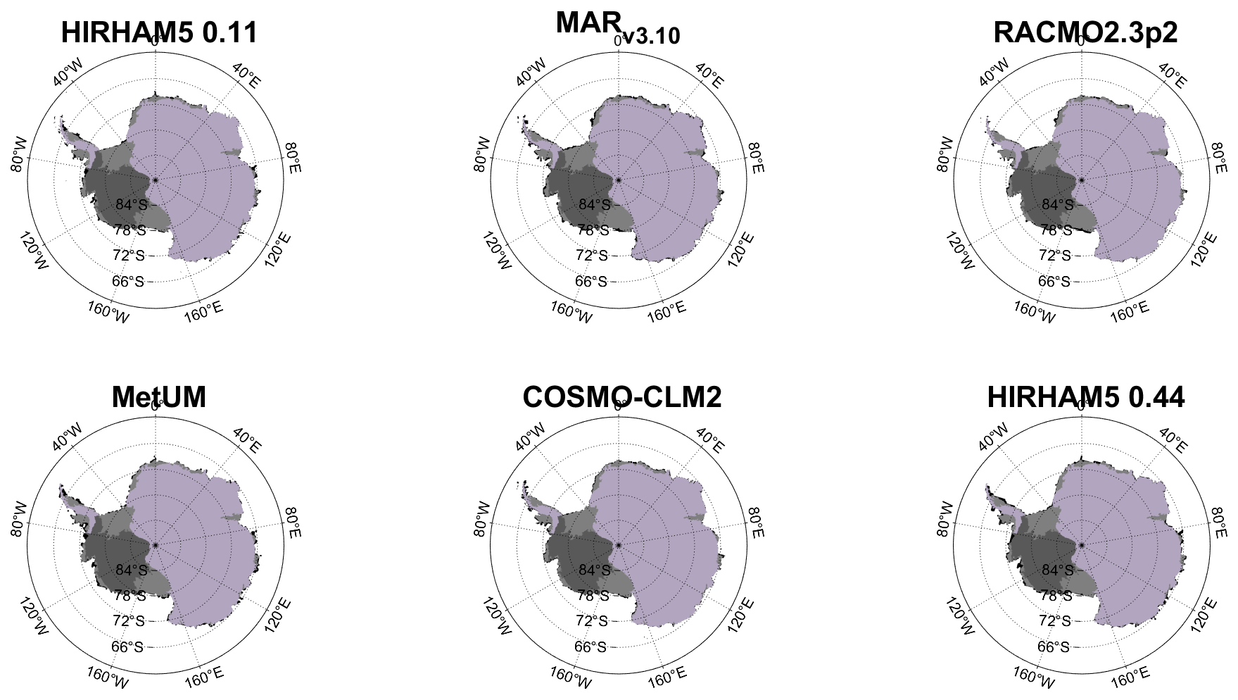
Figure A1Ice masks used in this study differ for each model, and we therefore define a common mask where all models have ice present in the domain. The sub-figures show where the common mask and the individual model masks are identical; black indicates where individual models have ice that does not occur in the common mask. Most models do not distinguish the physiography between ice shelves and grounded land ice. Overlaid is the regional mask for the grounded ice sheet as calculated by Rignot et al. (2019). Purple shows the grounded ice in the East Antarctic (EAIS) and Antarctic Peninsula (AP) regions; dark grey is the grounded West Antarctic (WAIS) ice sheet. Floating ice shelves within the common mask are shown in light grey.
Table A1Mean annual SMB for the grounded ice sheet over the total (GAIS), the East Antarctic (EAIS), West Antarctic (WAIS), and Antarctic Peninsula (AP) regions over the common mask for the common 1981–2016 period, where all the models overlap (except COSMO-CLM2, which is shown for 1987–2015). The ensemble mean is calculated only from models that cover the full period and therefore excludes the COSMO-CLM2 results but includes the driving ERA-Interim model. SMB here is calculated using the simple Eq. (1) to enable a fair comparison. We used the Rignot et al. (2019) definitions for the different regions of Antarctica.
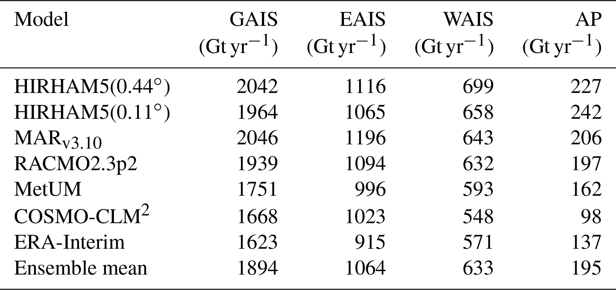
A2 Comparison with SMB observations
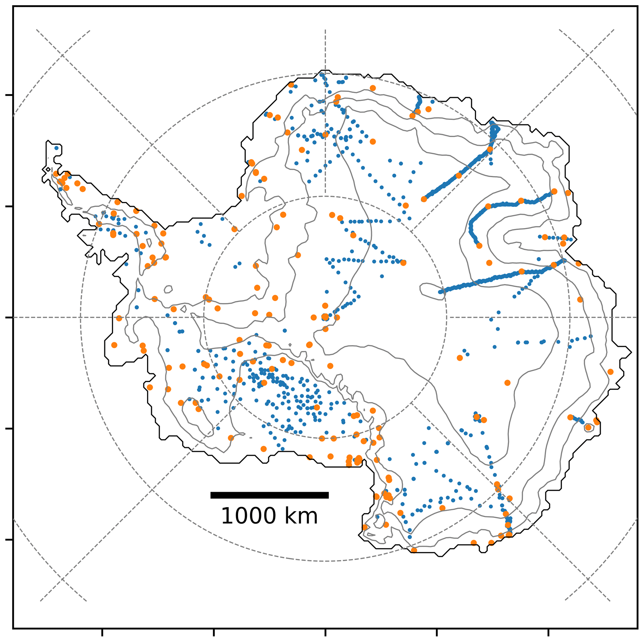
Figure A2Location of automatic weather stations and SMB observations in Antarctica and used in this study.
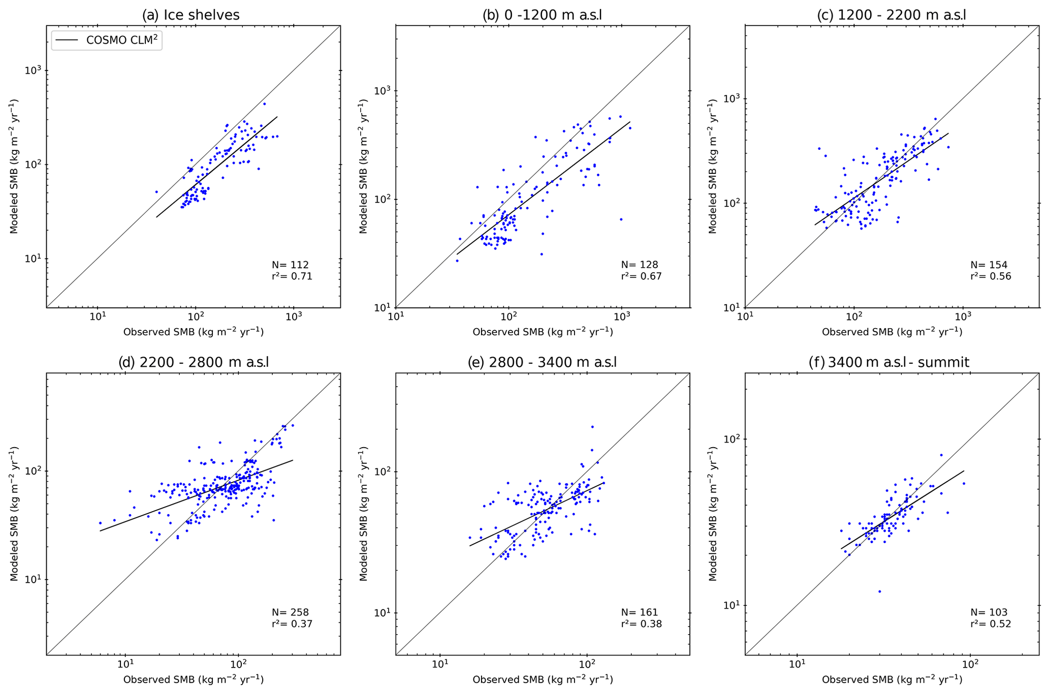
Figure A3Comparison between COSMO-CLM2 and observed SMB (units: kg m−2 yr−1) over the ice shelves (a) and by elevation classes (b–f). Due to the use of logarithmic axes, only positive values for the observed and modelled SMB from all the RCMs in this study are used (number for each bin N). Finally, the regression coefficient of each regression line is also shown (r2).
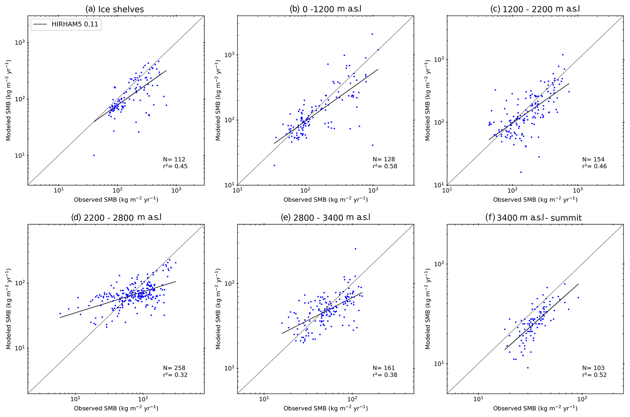
Figure A4Comparison between HIRHAM5 0.11∘ and observed SMB (units: kg m−2 yr−1) over the ice shelves (a) and by elevation classes (b–f). Due to the use of logarithmic axes, only positive values for the observed and modelled SMB from all the RCMs in this study are used (number for each bin N). Finally, the regression coefficient of each regression line is also shown (r2).
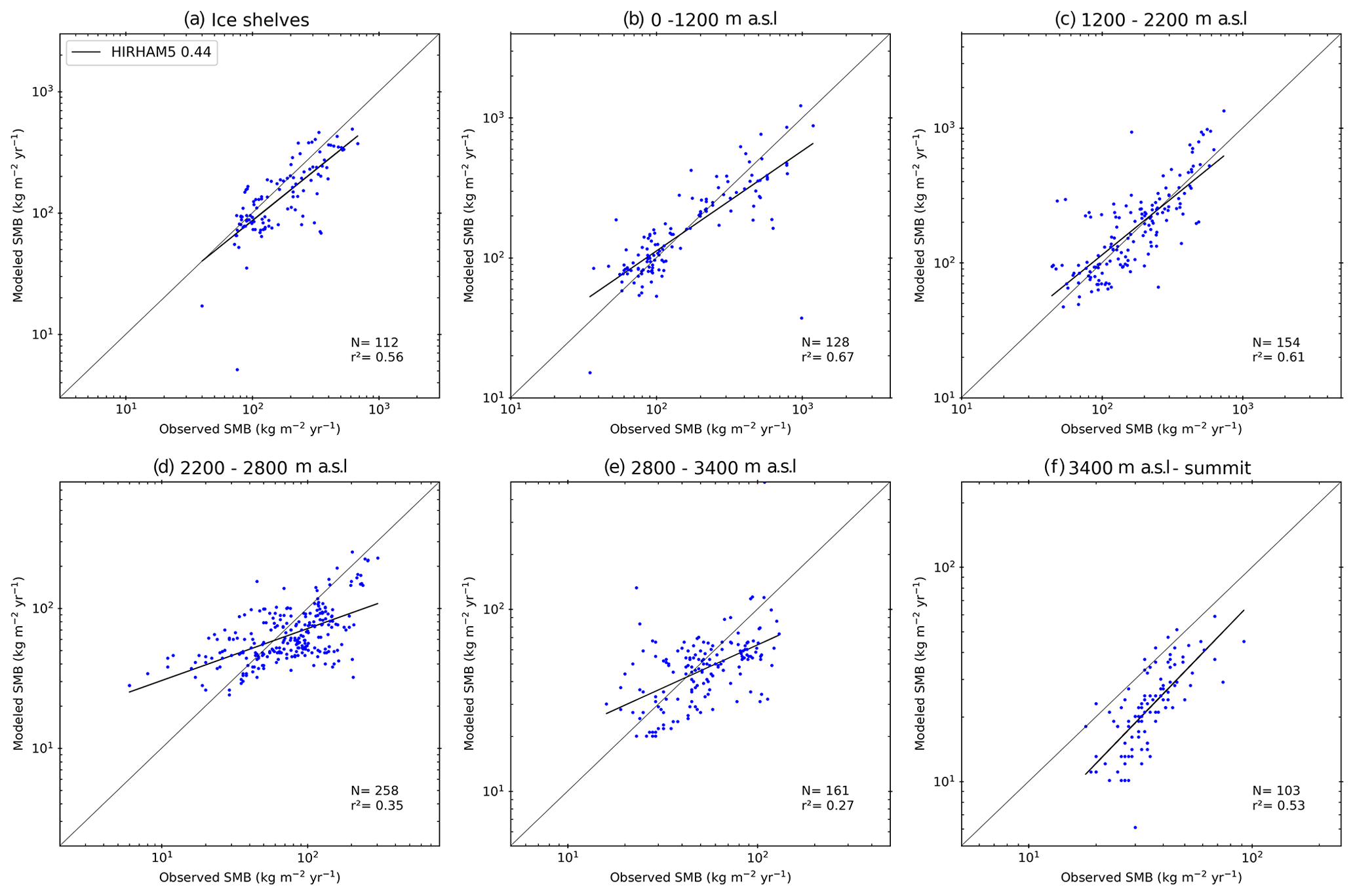
Figure A5Comparison between HIRHAM5 0.44∘ and observed SMB (units: kg m−2 yr−1) over the ice shelves (a) and by elevation classes (b–f). Due to the use of logarithmic axes, only positive values for the observed and modelled SMB from all the RCMs in this study are used (number for each bin N). Finally, the regression coefficient of each regression line is also shown (r2).
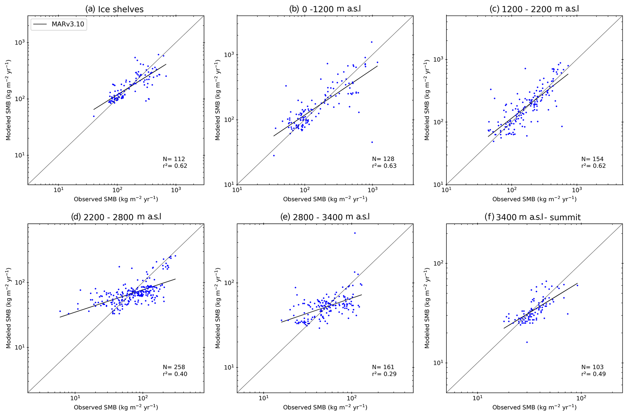
Figure A6Comparison between MARv3.10 and observed SMB (units: kg m−2 yr−1) over the ice shelves (a) and by elevation classes (b–f). Due to the use of logarithmic axes, only positive values for the observed and modelled SMB from all the RCMs in this study are used (number for each bin N). Finally, the regression coefficient of each regression line is also shown (r2).
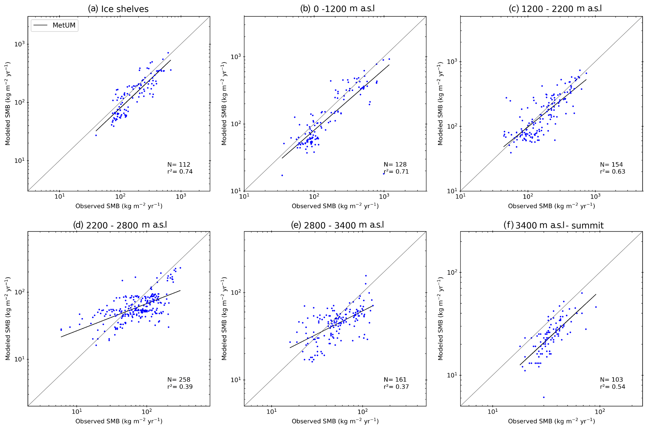
Figure A7Comparison between MetUM and observed SMB (units: kg m−2 yr−1) over the ice shelves (a) and by elevation classes (b–f). Due to the use of logarithmic axes, only positive values for the observed and modelled SMB from all the RCMs in this study are used (number for each bin N). Finally, the regression coefficient of each regression line is also shown (r2).
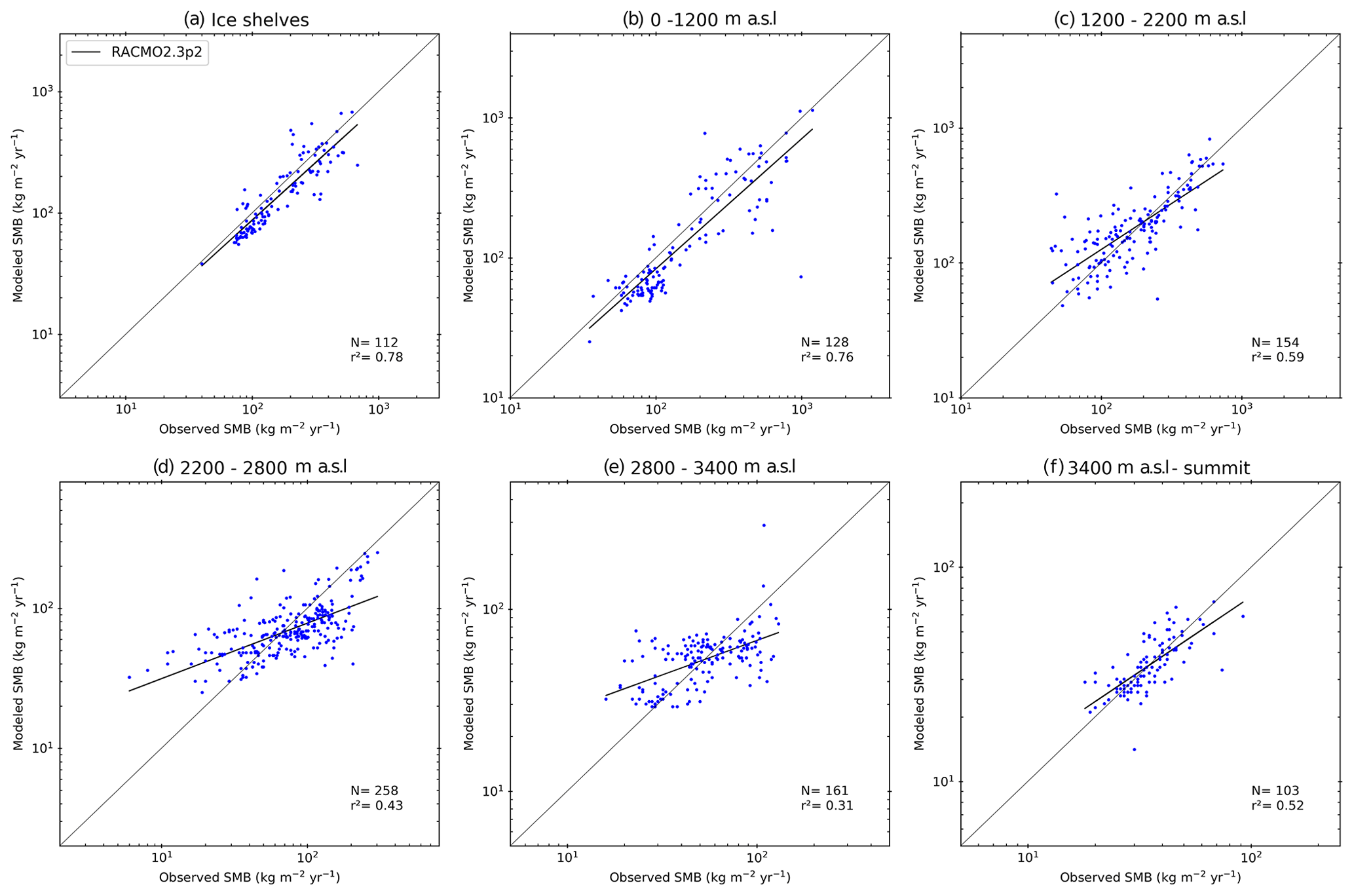
Figure A8Comparison between RACMO2.3p2 and observed SMB (units: kg m−2 yr−1) over the ice shelves (a) and by elevation classes (b–f). Due to the use of logarithmic axes, only positive values for the observed and modelled SMB from all the RCMs in this study are used (number for each bin N). Finally, the regression coefficient of each regression line is also shown (r2).
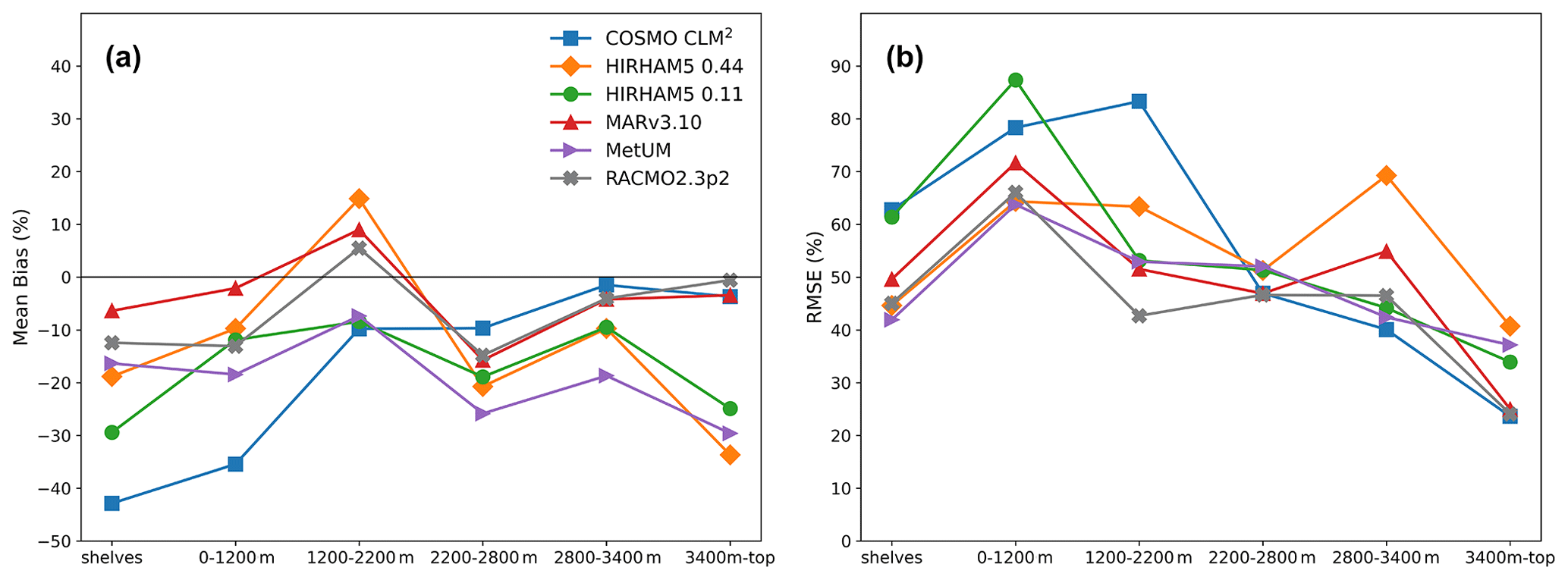
Model outputs used in this paper are available to download from the CORDEX archive; see https://www.cordex.org/data-access/how-to-access-the-data/ (CORDEX, 2021) for instructions. In addition The COSMO-CLM2 monthly output of key variables is open-access and available at https://doi.org/10.5281/zenodo.2539147 (Souverijns, 2019). Output for key variables from the high-resolution HIRHAM5 simulations is available here: http://ensemblesrt3.dmi.dk/data/prudence/temp/RUM/HIRHAM/ANTARCTICA/ERAI/ (Mottram and Boberg, 2021); further data are available on request. MAR3.10 monthly outputs are available here: https://doi.org/10.5281/zenodo.5195636 (Kittel et al., 2020); all other variables are available on request. Modelled SMB for the common period and broken down regionally for all models (see Appendix A1) is open-access and available on Zenodo: https://doi.org/10.5281/zenodo.4590263 (Mottram, 2021).
RM and SBS conceived the study. Analysis of simulations was carried out by CK, JMVW, NH, and RM. Model simulations were carried out by FB, CK, NS, AG, AO, SW, TP, JWVM, and EVM. All authors contributed to the paper.
The authors declare that they have no conflict of interest.
This article is part of the special issue “The Ice Sheet Model Intercomparison Project for CMIP6 (ISMIP6)”. It is not associated with a conference.
Acquisition of meteorological data in Adélie Land has been made with the financial and logistical support of the French Polar Institute IPEV (programme CALVA-1013). The authors appreciate the support of the University of Wisconsin-Madison Automatic Weather Station programme for the dataset, data display, and information (NSF grant no. 1924730).
The COSMO-CLM2 integrations were supported by the Belgian Science Policy Office (BELSPO; grant no. 747 BR/143/A2/AEROCLOUD) and the Research Foundation Flanders (FWO; grant nos. 748 G0C2215N and GOF5318N; EOS ID: 30454083). Computational resources and services were provided by the Flemish Supercomputer Center, funded by the FWO and the Flemish Government, EWI department. Matthias Demuzere, Jan Lenaerts, Irina Gorodetskaya, and Sam Vanden Broucke are gratefully acknowledged for supporting the COSMO-CLM2 integrations. COSMO-CLM2 is the community model of the German regional climate research jointly further developed by the CLM community. Computational resources for MAR simulations have been provided by the Consortium des Équipements de Calcul Intensif (CÉCI), funded by the Fonds de la Recherche Scientifique de Belgique (F.R.S. – FNRS) under grant no. 2.5020.11 and the Tier-1 supercomputer (Zenobe) of the Fédération Wallonie Bruxelles infrastructure funded by the Walloon Region under grant agreement no. 1117545. Christoph Kittel's work was supported by the Fonds de la Recherche Scientifique – FNRS under grant no. T.0002.16.
Melchior van Wessen, Willem Jan van de Berg, and Erik van Meijgaard acknowledge the ECMWF for the use of their computing and archive facilities for the RACMO2 simulations.
Ruth Mottram, Nicolaj Hansen, and Sebastian B. Simonsen acknowledge the ESA Climate Change Initiative for the Greenland ice sheet funded via ESA-ESRIN contract no. 4000104815/11/I-NB and the Sea Level Budget Closure CCI project funded via ESA-ESRIN contract no. 4000119910/17/I-NB. HIRHAM5 regional climate model simulations were carried out by Ruth Mottram and Fredrik Boberg as part of the ice2ice project, a European Research Council project under the European Community’s Seventh Framework Programme (FP7/ 2007–2013)/ ERC grant agreement 610055. Data analysis was supported by the Danish state through the National Centre for Climate Research (NCKF).
This publication was supported by PROTECT. This project has received funding from the European Union's Horizon 2020 research and innovation programme under grant agreement no. 869304 and PROTECT contribution number 19.
This paper was edited by Ayako Abe-Ouchi and reviewed by Jan Lenaerts, Masashi Niwano, and one anonymous referee.
Agosta, C., Fettweis, X., and Datta, R.: Evaluation of the CMIP5 models in the aim of regional modelling of the Antarctic surface mass balance, The Cryosphere, 9, 2311–2321, https://doi.org/10.5194/tc-9-2311-2015, 2015. a
Agosta, C., Amory, C., Kittel, C., Orsi, A., Favier, V., Gallée, H., van den Broeke, M. R., Lenaerts, J. T. M., van Wessem, J. M., van de Berg, W. J., and Fettweis, X.: Estimation of the Antarctic surface mass balance using the regional climate model MAR (1979–2015) and identification of dominant processes, The Cryosphere, 13, 281–296, https://doi.org/10.5194/tc-13-281-2019, 2019. a, b, c, d, e, f, g, h, i, j, k, l
Akperov, M., Rinke, A., Mokhov, I. I., Matthes, H., Semenov, V. A., Adakudlu, M., Cassano, J., Christensen, J. H., Dembitskaya, M. A., Dethloff, K., Fettweis, X., Glisan, J., Gutjahr, O., Heinemann, G., Koenigk, T., Koldunov, N. V., Laprise, R., Mottram, R., Nikiéma, O., Scinocca, J. F., Sein, D., Sobolowski, S., Winger, K., and Zhang, W.: Cyclone Activity in the Arctic From an Ensemble of Regional Climate Models (Arctic CORDEX), 123, 2537–2554, https://doi.org/10.1002/2017JD027703, 2018. a, b
Alexandru, A., de Elia, R., Laprise, R., Separovic, L., and Biner, S.: Sensitivity Study of Regional Climate Model Simulations to Large-Scale Nudging Parameters, Mon. Weather Rev., 137, 1666–1686, https://doi.org/10.1175/2008MWR2620.1, 2009. a
Amory, C.: Drifting-snow statistics from multiple-year autonomous measurements in Adélie Land, East Antarctica, The Cryosphere, 14, 1713–1725, https://doi.org/10.5194/tc-14-1713-2020, 2020. a
Andersen, K. K., Ditlevsen, P. D., Rasmussen, S. O., Clausen, H. B., Vinther, B. M., Johnsen, S. J., and Steffensen, J. P.: Retrieving a common accumulation record from Greenland ice cores for the past 1800 years, J. Geophys. Res.-Atmos., 111, D15106, https://doi.org/10.1029/2005JD006765., 2006. a, b
Bamber, J. L.: A digital elevation model of the Antarctic ice sheet derived from ERS-1 altimeter data and comparison with terrestrial measurements, Annals Glaciology, 20, 48–54, 1994. a
Bamber, J. L., Gomez-Dans, J. L., and Griggs, J. A.: A new 1 km digital elevation model of the Antarctic derived from combined satellite radar and laser data – Part 1: Data and methods, The Cryosphere, 3, 101–111, https://doi.org/10.5194/tc-3-101-2009, 2009 a
Barthel, A., Agosta, C., Little, C. M., Hattermann, T., Jourdain, N. C., Goelzer, H., Nowicki, S., Seroussi, H., Straneo, F., and Bracegirdle, T. J.: CMIP5 model selection for ISMIP6 ice sheet model forcing: Greenland and Antarctica, The Cryosphere, 14, 855–879, https://doi.org/10.5194/tc-14-855-2020, 2020. a
Berg, P., Döscher, R., and Koenigk, T.: Impacts of using spectral nudging on regional climate model RCA4 simulations of the Arctic, Geosci. Model Dev., 6, 849–859, https://doi.org/10.5194/gmd-6-849-2013, 2013. a, b
Brun, E., David, P., Subul, M., and Brunot, G.: A numerical model to simulate snow-cover stratigraphy for operational avalanche forescating, J. Glaciol., 38, 13–22, 1992. a
Christensen, O., Gutowski, W., Nikulin, G., and Legutke, S.: CORDEX Archive design, Danish Meteorological Institute, Copenhagen, Denmark, 2014. a
Cogley, J. G., Hock, R., Rasmussen, L. A., Arendt, A. A., Bauder, A., Braithwaite, R. J., Jansson, P., Kaser, G., Möller, M., Nicholson, L., and Zemp, M.: Glossary of Glacier Mass Balance and Related Terms, IHP-VII Technical Documents in Hydrology No. 86, IACS Contribution No. 2, UNESCO-IHP, Paris, France, 114 pp., 2010. a
Cook, A. J., Murray, T., Luckman, A., Vaughan, D. G., and Barrand, N. E.: A new 100-m Digital Elevation Model of the Antarctic Peninsula derived from ASTER Global DEM: methods and accuracy assessment, Earth Syst. Sci. Data, 4, 129–142, https://doi.org/10.5194/essd-4-129-2012, 2012a. a
Cook, A. J., Murray, T., Luckman, A., Vaughan, D. G., and Barrand, N. E.: Antarctic Peninsula 100 m Digital Elevation Model Derived from ASTER GDEM, Boulder, Colorado, USA, National Snow and Ice Data Center, https://doi.org/10.7265/N58K7711, 2012b. a
CORDEX: The World Climate Research Programme Project “Co-Ordinated Regional Downscaling Experiment”, available at: https://cordex.org/data-access/how-to-access-the-data/, last access: 1 June 2021. a
Cox, P., Betts, R., Bunton, C., Essery, R., Rowntree, P., and Smith, J.: The impact of new land surface physics on the GCM simulation of climate and climate sensitivity, Clim. Dynam., 15, 183–203, 1999. a
Das, I., Bell, R. E., Scambos, T. A., Wolovick, M., Creyts, T. T., Studinger, M., Frearson, N., Nicolas, J. P., Lenaerts, J. T., and Van Den Broeke, M. R.: Influence of persistent wind scour on the surface mass balance of Antarctica, Nat. Geosci., 6, 367–371, https://doi.org/10.1038/ngeo1766, 2013 a
De Ridder, K. and Gallée, H.: Land surface-induce regional climate change in Southern Israel, J. Appl. Meteorol., 37, 1470–1485, 1998. a
DeConto, R. and Pollard, D.: Contribution of Antarctica to past and future sea-level rise, Nature, 531, 591–597, https://doi.org/10.1038/nature17145, 2016. a
Dee, D. P., Uppala, S. M., Simmons, A. J., Berrisford, P., Poli, P., Kobayashi, S., Andrae, U., Balmaseda, M. A., Balsamo, G., Bauer, P., Bechtold, P., Beljaars, A. C. M., van de Berg, L., Bidlot, J., Bormann, N., Delsol, C., Dragani, R., Fuentes, M., Geer, A. J., Haimberger, L., Healy, S. B., Hersbach, H., Hólm, E. V., Isaksen, L., Kållberg, P., Köhler, M., Matricardi, M., McNally, A. P., Monge-Sanz, B. M., Morcrette, J.-J., Park, B.-K., Peubey, C., de Rosnay, P., Tavolato, C., Thépaut, J.-N., and Vitart, F.: The ERA-Interim reanalysis: configuration and performance of the data assimilation system, Q. J. Roy. Meteor. Soc., 137, 553–597, https://doi.org/10.1002/qj.828, 2011. a, b, c
Edwards, T. L., Brandon, M. A., Durand, G., Edwards, N. R., Golledge, N. R., Holden, P. B., Nias, I. J., Payne, A. J., Ritz, C., and Wernecke, A.: Revisiting Antarctic ice loss due to marine ice-cliff instability, Nature, 566, 58–64, https://doi.org/10.1038/s41586-019-0901-4, 2019. a
Earth Resources Observation and Science Center/U.S. Geological Survey/U.S. Department of the Interior: USGS 30 ARC-second Global Elevation Data, GTOPO30, Research Data Archive at the National Center for Atmospheric Research, Computational and Information Systems Laboratory, https://doi.org/10.5065/A1Z4-EE71, 1997. a
Eerola, K.: About the performance of HIRLAM version 7.0, Hirlam Newsletter, 51, 93–102, available at: https://hirlam.org/index.php/hirlam-documentation/doc_view/473-hirlam-newsletter-no-51-article14-eerola-performance-hirlam7-0 (last access: 1 June 2021), 2006. a
Ettema, J., van den Broeke, M. R., van Meijgaard, E., and van de Berg, W. J.: Climate of the Greenland ice sheet using a high-resolution climate model – Part 2: Near-surface climate and energy balance, The Cryosphere, 4, 529–544, https://doi.org/10.5194/tc-4-529-2010, 2010. a
Favier, V., Agosta, C., Parouty, S., Durand, G., Delaygue, G., Gallée, H., Drouet, A.-S., Trouvilliez, A., and Krinner, G.: An updated and quality controlled surface mass balance dataset for Antarctica, The Cryosphere, 7, 583–597, https://doi.org/10.5194/tc-7-583-2013, 2013. a
Fettweis, X., Box, J. E., Agosta, C., Amory, C., Kittel, C., Lang, C., van As, D., Machguth, H., and Gallée, H.: Reconstructions of the 1900–2015 Greenland ice sheet surface mass balance using the regional climate MAR model, The Cryosphere, 11, 1015–1033, https://doi.org/10.5194/tc-11-1015-2017, 2017. a
Forbes, R., Tompkins, A., and Ungatch, A.: A new prognostic bulk microphysics scheme for the IFS, Technical Memorandum 649, ECMWF, available at: http://www.ecmwf.int/sites/default/files/elibrary/2011/9441-new-prognostic-bulk-microphysics-scheme-ifs.pdf (last access: 1 June 2021), 2011. a
Franco, B., Fettweis, X., Lang, C., and Erpicum, M.: Impact of spatial resolution on the modelling of the Greenland ice sheet surface mass balance between 1990–2010, using the regional climate model MAR, The Cryosphere, 6, 695–711, https://doi.org/10.5194/tc-6-695-2012, 2012. a
Fretwell, P., Pritchard, H. D., Vaughan, D. G., Bamber, J. L., Barrand, N. E., Bell, R., Bianchi, C., Bingham, R. G., Blankenship, D. D., Casassa, G., Catania, G., Callens, D., Conway, H., Cook, A. J., Corr, H. F. J., Damaske, D., Damm, V., Ferraccioli, F., Forsberg, R., Fujita, S., Gim, Y., Gogineni, P., Griggs, J. A., Hindmarsh, R. C. A., Holmlund, P., Holt, J. W., Jacobel, R. W., Jenkins, A., Jokat, W., Jordan, T., King, E. C., Kohler, J., Krabill, W., Riger-Kusk, M., Langley, K. A., Leitchenkov, G., Leuschen, C., Luyendyk, B. P., Matsuoka, K., Mouginot, J., Nitsche, F. O., Nogi, Y., Nost, O. A., Popov, S. V., Rignot, E., Rippin, D. M., Rivera, A., Roberts, J., Ross, N., Siegert, M. J., Smith, A. M., Steinhage, D., Studinger, M., Sun, B., Tinto, B. K., Welch, B. C., Wilson, D., Young, D. A., Xiangbin, C., and Zirizzotti, A.: Bedmap2: improved ice bed, surface and thickness datasets for Antarctica, The Cryosphere, 7, 375–393, https://doi.org/10.5194/tc-7-375-2013, 2013. a
Gallée, H. and Schayes, G.: Development of a Three-Dimensional Meso-γ Primitive Equation Model: Katabatic Winds Simulation in the Area of Terra Nova Bay, Antarctica, Mon. Weather Rev., 122, 671–685, https://doi.org/10.1175/1520-0493(1994)122<0671:DOATDM>2.0.CO;2, 1994. a
GLOBE Task Team and others (Hastings, D. A., Dunbar, P. K., Elphingstone, G. M., Bootz, M., Murakami, H., Maruyama, H., Masaharu, H., Holland, P., Payne, J., Bryant, N. A., Logan, T. L., Muller, J.-P., Schreier, G., and MacDonald, J. S.), eds.: The Global Land One-kilometer Base Elevation (GLOBE) Digital Elevation Model, Version 1.0, National Oceanic and Atmospheric Administration, National Geophysical Data Center, 325 Broadway, Boulder, Colorado 80305-3328, USA, Digital data base on the World Wide Web, available at: http://www.ngdc.noaa.gov/mgg/topo/globe.html (last access: 1 June 2021) and CD-ROMs, 1999. a
Hansen, N.: Modelling the present day and future climate of Antarctica, Master's thesis, The Technical University of Denmark, Anker Engelunds Vej 1 Bygning 101A 2800 Kgs. Lyngby, Denmark, 2019. a
Hermann, M., Box, J. E., Fausto, R. S., Colgan, W. T., Langen, P. L., Mottram, R., Wuite, J., Noël, B., van den Broeke, M. R., and van As, D.: Application of PROMICE Q-Transect in Situ Accumulation and Ablation Measurements (2000–2017) to Constrain Mass Balance at the Southern Tip of the Greenland Ice Sheet, J. Geophys. Res.-Earth, 123, 1235–1256, https://doi.org/10.1029/2017JF004408, 2018. a, b, c
Kittel, C., Amory, C., Agosta, C., Delhasse, A., Doutreloup, S., Huot, P.-V., Wyard, C., Fichefet, T., and Fettweis, X.: Sensitivity of the current Antarctic surface mass balance to sea surface conditions using MAR, The Cryosphere, 12, 3827–3839, https://doi.org/10.5194/tc-12-3827-2018, 2018. a, b, c
Kittel, C., Amory, C., Agosta, C., and Fettweis, X.: MARv3.10 outputs: What is the Surface Mass Balance of Antarctica? An Intercomparison of Regional Climate Model Estimates [data set], Zenodo, https://doi.org/10.5281/zenodo.5195636, 2020. a
Kittel, C.: Present and future sensitivity of the Antarctic surface mass balance to oceanic and atmospheric forcings: insights with the regional climate model MAR, PhD thesis, Université de Liège, Liège, Belgique, available at: https://orbi.uliege.be/handle/2268/258491, last access: 1 June 2021. a
Krinner, G., Guicherd, B., Ox, K., Genthon, C., and Magand, O.: Influence of oceanic boundary conditions in simulations of Antarctic climate and surface mass balance change during the coming century, J. Climate, 21, 938–962, 2008. a
Kuipers Munneke, P., Van den Broeke, M., Lenaerts, J., Flanner, M., Gardner, A., and Van de Berg, W.: A new albedo parameterization for use in climate models over the Antarctic ice sheet, J. Geophys. Res.-Atmos., 116, D05114, https://doi.org/10.1029/2010JD015113, 2011. a
Langen, P. L., Fausto, R. S., Vandecrux, B., Mottram, R. H., and Box, J. E.: Liquid water flow and retention on the Greenland ice sheet in the regional climate model HIRHAM5: Local and large-scale impacts, Front. Earth Sci., 4, 110, https://doi.org/10.3389/feart.2016.00110, 2017. a
Lenaerts, J. T., Van den Broeke, M., Déry, S., Van Meijgaard, E., Van de Berg, W., Palm, S. P., and Sanz Rodrigo, J.: Modeling drifting snow in Antarctica with a regional climate model: 1. Methods and model evaluation, J. Geophys. Res.-Atmos., 117, D05108, https://doi.org/10.1029/2011JD016145, 2012a. a
Lenaerts, J. T., Van Den Broeke, M. R., Scarchilli, C., and Agosta, C.: Impact of model resolution on simulated wind, drifting snow and surface mass balance in Terre Adélie, East Antarctica, J. Glaciol., 58, 821–829, 2012b. a
Lenaerts, J. T., Vizcaino, M., Fyke, J., Van Kampenhout, L., and van den Broeke, M. R.: Present-day and future Antarctic ice sheet climate and surface mass balance in the Community Earth System Model, Clim. Dynam., 47, 1367–1381, 2016. a
Lenaerts, J. T., Medley, B., van den Broeke, M. R., and Wouters, B.: Observing and Modeling Ice-Sheet Surface Mass Balance, Rev. Geophys., 376–420, https://doi.org/10.1029/2018RG000622, 2019. a, b
Ligtenberg, S. R. M., Helsen, M. M., and van den Broeke, M. R.: An improved semi-empirical model for the densification of Antarctic firn, The Cryosphere, 5, 809–819, https://doi.org/10.5194/tc-5-809-2011, 2011. a
Liu, H., Jezek, K. C., Li, B., and Zhao, Z.: Radarsat Antarctic Mapping Project Digital Elevation Model, Version 2, Boulder, Colorado USA, NASA National Snow and Ice Data Center Distributed Active Archive Center, https://doi.org/10.5067/8JKNEW6BFRVD, 2015. a
Lucas-Picher, P., Wulff-Nielsen, M., Christensen, J. H., Aðalgeirsdóttir, G., Mottram, R., and Simonsen, S. B.: Very high resolution regional climate model simulations over Greenland: Identifying added value, J. Geophys. Res.-Atmos., 117, https://doi.org/10.1029/2011JD016267, 2012. a, b
Medley, B., Joughin, I., Smith, B. E., Das, S. B., Steig, E. J., Conway, H., Gogineni, S., Lewis, C., Criscitiello, A. S., McConnell, J. R., van den Broeke, M. R., Lenaerts, J. T. M., Bromwich, D. H., Nicolas, J. P., and Leuschen, C.: Constraining the recent mass balance of Pine Island and Thwaites glaciers, West Antarctica, with airborne observations of snow accumulation, The Cryosphere, 8, 1375–1392, https://doi.org/10.5194/tc-8-1375-2014, 2014. a
Mikkelsen, T. B., Grinsted, A., and Ditlevsen, P.: Influence of temperature fluctuations on equilibrium ice sheet volume, The Cryosphere, 12, 39–47, https://doi.org/10.5194/tc-12-39-2018, 2018. a
Mottram, R.: Regional Surface Mass Balance of Antarctica (1981–2016) estimated from five high resolution Regional Climate Models (Version 1.0) [Data set], Zenodo, https://doi.org/10.5281/zenodo.4590263, 2021. a
Mottram, R. and Boberg, F.: Atmospheric climate model output from the regional climate model HIRHAM5 forced with ERA-Interim for Antarctica, available at: http://ensemblesrt3.dmi.dk/data/prudence/temp/RUM/HIRHAM/ANTARCTICA/ERAI/, last access: 1 June 2021. a
Nowicki, S. M. J., Payne, A., Larour, E., Seroussi, H., Goelzer, H., Lipscomb, W., Gregory, J., Abe-Ouchi, A., and Shepherd, A.: Ice Sheet Model Intercomparison Project (ISMIP6) contribution to CMIP6, Geosci. Model Dev., 9, 4521–4545, https://doi.org/10.5194/gmd-9-4521-2016, 2016. a
Oleson, K. W. and Lawrence, D. M.: Technical description of version 4.5 of the Community Land Model (CLM), Tech. Rep. July, NCAR, Boulder, Colorado, https://doi.org/10.5065/D6RR1W7M, 2013. a
Oppenheimer, M., Glavovic, B. C., Hinkel, J., van de Wal, R., Magnan, A. K., Abd-Elgawad, A., Cai, R., Cifuentes-Jara, M., DeConto, R. M., Ghosh, T., Hay, J., Isla, F., Marzeion, B., Meyssignac, B., and Sebesvari, Z.: Sea Level Rise and Implications for Low-Lying Islands, Coasts and Communities, in: IPCC Special Report on the Ocean and Cryosphere in a Changing Climate, edited by: Pörtner, H.-O., Roberts, D. C., Masson-Delmotte, V., Zhai, P., Tignor, M., Poloczanska, E., Mintenbeck, K., Alegría, A., Nicolai, M., Okem, A., Petzold, J., Rama, B., and Weyer, N. M., Cambridge University Press, Cambridge, UK, 126 pp., 2019. a
Orr, A., Hosking, J. S., Hoffmann, L., Keeble, J., Dean, S. M., Roscoe, H. K., Abraham, N. L., Vosper, S., and Braesicke, P.: Inclusion of mountain-wave-induced cooling for the formation of PSCs over the Antarctic Peninsula in a chemistry–climate model, Atmos. Chem. Phys., 15, 1071–1086, https://doi.org/10.5194/acp-15-1071-2015, 2015. a
Rignot, E., Velicogna, I., van den Broeke, M. R., Monaghan, A., and Lenaerts, J. T.: Acceleration of the contribution of the Greenland and Antarctic ice sheets to sea level rise, Geophys. Res. Lett., 38, https://doi.org/10.1029/2011GL046583, 2011. a
Rignot, E., Mouginot, J., Scheuchl, B., Broeke, M. v. d., Wessem, M. J. v., and Morlighem, M.: Four decades of Antarctic Ice Sheet mass balance from 1979–2017, P. Natl. Acad. Sci. USA, 116, 1095–1103, https://doi.org/10.1073/pnas.1812883116, 2019. a, b, c, d, e, f, g, h, i
Robel, A. A., Seroussi, H., and Roe, G. H.: Marine ice sheet instability amplifies and skews uncertainty in projections of future sea-level rise, P. Natl. Acad. Sci. USA, 116, 14887–14892, 2019. a
Rockel, B., Will, A., and Hense, A.: The Regional Climate Model COSMO-CLM (CCLM), Meteorologische Zeitschrift, 17, 347–348, https://doi.org/10.1127/0941-2948/2008/0309, 2008. a
Roeckner, E., Bäuml, G., Bonaventura, L., Brokopf, R., Esch, M., Giorgetta, M., Hagemann, S., Kirchner, I., Kornblueh, L., Manzini, E., Rhodin, A., Schlese, U., Schulzweida, U., and Tompkins, A: The atmospheric general circulation model ECHAM 5. PART I: Model description, Max Planck Institute, Hamburg, Germany, 2003. a
Scambos, T. and Shuman, C.: Comment on “Mass gains of the Antarctic ice sheet exceed losses” by Zwally, H. J. and others, J. Glaciol., 62, 599–603, https://doi.org/10.1017/jog.2016.59, 2016. a
Scambos, T., Frezzotti, M., Haran, T., Bohlander, J., Lenaerts, J., van Den Broeke, M., Jezek, K., Long, D., Urbini, S., Farness, K., Neumann, T., Albert, M., and Winther, J.: Extent of low-accumulation “wind glaze” areas on the East Antarctic plateau: implications for continental ice mass balance, J. Glaciol., 58, 633–647, https://doi.org/10.3189/2012JoG11J232, 2012. a
Schmidt, L. S., Aðalgeirsdóttir, G., Guðmundsson, S., Langen, P. L., Pálsson, F., Mottram, R., Gascoin, S., and Björnsson, H.: The importance of accurate glacier albedo for estimates of surface mass balance on Vatnajökull: evaluating the surface energy budget in a regional climate model with automatic weather station observations, The Cryosphere, 11, 1665–1684, https://doi.org/10.5194/tc-11-1665-2017, 2017. a, b, c
Sedlar, J., Tjernström, M., Mauritsen, T., Shupe, M. D., Brooks, I. M., Persson, P. O. G., Birch, C. E., Leck, C., Sirevaag, A., and Nicolaus, M.: A transitioning Arctic surface energy budget: the impacts of solar zenith angle, surface albedo and cloud radiative forcing, Clim. Dynam., 37, 1643–1660, 2011. a
Shepherd, A., Fricker, H. A., and Farrell, S. L.: Trends and connections across the Antarctic cryosphere, Nature, 558, 223–232, https://doi.org/10.1038/s41586-018-0171-6, 2018. a, b
Shepherd, A., Ivins, E., Rignot, E., Smith, B., van den Broeke, M., Velicogna, I., Whitehouse, P., Briggs, K., Joughin, I., Krinner, G., Nowicki, S., Payne, T., Scambos, T., Schlegel, N., A, G., Agosta, C., Ahlstrøm, A., Babonis, G., Barletta, V. R., Bjørk, A. A., Blazquez, A., Bonin, J., Colgan, W., Csatho, B., Cullather, R., Engdahl, M. E., Felikson, D., Fettweis, X., Forsberg, R., Hogg, A. E., Gallee, H., Gardner, A., Gilbert, L., Gourmelen, N., Groh, A., Gunter, B., Hanna, E., Harig, C., Helm, V., Horvath, A., Horwath, M., Khan, S., Kjeldsen, K. K., Konrad, H., Langen, P. L., Lecavalier, B., Loomis, B., Luthcke, S., McMillan, M., Melini, D., Mernild, S., Mohajerani, Y., Moore, P., Mottram, R., Mouginot, J., Moyano, G., Muir, A., Nagler, T., Nield, G., Nilsson, J., Noël, B., Otosaka, I., Pattle, M. E., Peltier, W. R., Pie, N., Rietbroek, R., Rott, H., Sandberg Sørensen, L., Sasgen, I., Save, H., Scheuchl, B., Schrama, E., Schröder, L., Seo, K.-W., Simonsen, S. B., Slater, T., Spada, G., Sutterley, T., Talpe, M., Tarasov, L., van de Berg, W. J., van der Wal, W., van Wessem, M., Vishwakarma, B. D., Wiese, D., Wilton, D., Wagner, T., Wouters, B., Wuite, J., and The IMBIE Team: Mass balance of the Greenland Ice Sheet from 1992 to 2018, Nature, 579, 233–239, https://doi.org/10.1038/s41586-019-1855-2, 2020. a, b, c, d, e, f, g, h, i
Shepherd, A., Gilbert, L., Muir, A. S., Konrad, H., McMillan, M., Slater, T., Briggs, K. H., Sundal, A. V., Hogg, A. E., and Engdahl, M.: Trends in Antarctic Ice Sheet Elevation and Mass, Geophys. Res. Lett., 46, 8174–8183, https://doi.org/10.1029/2019GL082182, 2019. a
Souverijns, N., Gossart, A., Demuzere, M., Lenaerts, J. T. M., Medley, B., Gorodetskaya, I. V., Vanden Broucke, S., and van Lipzig, N. P. M.: A New Regional Climate Model for POLAR-CORDEX: Evaluation of a 30-Year Hindcast with COSMO-CLM2 Over Antarctica, J. Geophys. Res.-Atmos., 124, 1405–1427, https://doi.org/10.1029/2018JD028862, 2019. a, b, c, d, e
Souverijns, N., Gossart, A., Demuzere, M., Lenaerts, J. T. M., Medley, B., Gorodetskaya, I. V., Vanden Broucke, S., and van Lipzig, N. P. M.: Atmospheric climate model output of the COSMO-CLM2 regional climate model hindcast run over Antarctica (1987–2016) (Version COSMO-CLM version 5.0_clm6 – Community Land Model version 4.5), Data set, Zenodo, https://doi.org/10.5281/zenodo.2539147, 2019. a
Stokes, C. R., Sanderson, J. E., Miles, B. W., Jamieson, S. S., and Leeson, A. A.: Widespread distribution of supraglacial lakes around the margin of the East Antarctic Ice Sheet, Sci. Rep., 9, 1–14, 2019. a
Sutter, J., Gierz, P., Grosfeld, K., Thoma, M., and Lohmann, G.: Ocean temperature thresholds for Last Interglacial West Antarctic Ice Sheet collapse, Geophys. Res. Lett., 43, 2675–2682, 2016. a
Thomas, E. R., van Wessem, J. M., Roberts, J., Isaksson, E., Schlosser, E., Fudge, T. J., Vallelonga, P., Medley, B., Lenaerts, J., Bertler, N., van den Broeke, M. R., Dixon, D. A., Frezzotti, M., Stenni, B., Curran, M., and Ekaykin, A. A.: Regional Antarctic snow accumulation over the past 1000 years, Clim. Past, 13, 1491–1513, https://doi.org/10.5194/cp-13-1491-2017, 2017. a
Trusel, L. D., Das, S. B., Osman, M. B., Evans, M. J., Smith, B. E., Fettweis, X., McConnell, J. R., Noël, B. P., and van den Broeke, M. R.: Nonlinear rise in Greenland runoff in response to post-industrial Arctic warming, Nature, 564, 104–108, https://doi.org/10.1038/s41586-018-0752-4, 2018. a
Turner, J., Colwell, S. R., Marshall, G. J., Lachlan-Cope, T. A., Carleton, A. M., Jones, P. D., Lagun, V., Reid, P. A., and Iagovkina, S.: The SCAR READER project: toward a high-quality database of mean Antarctic meteorological observations, J. Climate, 17, 2890–2898, 2004. a
Undén, P., Rontu, L., Järvinen, H., Lynch, P., Calvo, J., Cats, G., Cuxart, J., Eerola, K., Fortelius, C., Garcia-Moya, J.-A., Jones, C., Lenderlink, G., McDonald, A., McGrath, R., Navascués, B., Nielsen, N.-W., Odegaard, V., Rodríguez, E., Rummukainen, M., Rõõm, R., Sattler, K., Sass, B.-H., Savijärvi, H., Schreur, B.-W., Sigg, R., The, H., and Tijm, A.: HIRLAM-5 Scientific Documentation, available at: http://hirlam.org/index.php/hirlam-documentation/doc_download/308-unden-et-al-2002 (last access: 1 June 2021), 2002 a
van de Berg, W. J. and Medley, B.: Brief Communication: Upper-air relaxation in RACMO2 significantly improves modelled interannual surface mass balance variability in Antarctica, The Cryosphere, 10, 459–463, https://doi.org/10.5194/tc-10-459-2016, 2016. a, b, c
van Kampenhout, L., Lenaerts, J. T. M., Lipscomb, W. H., Sacks, W. J., Lawrence, D. M., Slater, A. G., and van den Broeke, M. R.: Improving the Representation of Polar Snow and Firn in the Community Earth System Model, J. Adv. Model. Earth Syst., 9, 2583–2600, https://doi.org/10.1002/2017MS000988, 2017. a
van Wessem, J. M., Reijmer, C. H., Morlighem, M., Mouginot, J., Rignot, E., Medley, B., Joughin, I., Wouters, B., Depoorter, M. A., Bamber, J. L., Lenaerts, J. T. M., De Van Berg, W. J., Van Den Broeke, M. R., and Van Meijgaard, E.: Improved representation of East Antarctic surface mass balance in a regional atmospheric climate model, J. Glaciol., 60, 761–770, https://doi.org/10.3189/2014JoG14J051, 2014. a, b, c, d, e, f, g
van Wessem, J. M., Reijmer, C. H., Lenaerts, J. T. M., van de Berg, W. J., van den Broeke, M. R., and van Meijgaard, E.: Updated cloud physics in a regional atmospheric climate model improves the modelled surface energy balance of Antarctica, The Cryosphere, 8, 125–135, https://doi.org/10.5194/tc-8-125-2014, 2014. a, b
van Wessem, J. M., van de Berg, W. J., Noël, B. P. Y., van Meijgaard, E., Amory, C., Birnbaum, G., Jakobs, C. L., Krüger, K., Lenaerts, J. T. M., Lhermitte, S., Ligtenberg, S. R. M., Medley, B., Reijmer, C. H., van Tricht, K., Trusel, L. D., van Ulft, L. H., Wouters, B., Wuite, J., and van den Broeke, M. R.: Modelling the climate and surface mass balance of polar ice sheets using RACMO2 – Part 2: Antarctica (1979–2016), The Cryosphere, 12, 1479–1498, https://doi.org/10.5194/tc-12-1479-2018, 2018. a, b, c, d, e, f
Vernon, C. L., Bamber, J. L., Box, J. E., van den Broeke, M. R., Fettweis, X., Hanna, E., and Huybrechts, P.: Surface mass balance model intercomparison for the Greenland ice sheet, The Cryosphere, 7, 599–614, https://doi.org/10.5194/tc-7-599-2013, 2013. a
von Storch, H., Langenberg, H., and Feser, F.: A Spectral Nudging Technique for Dynamical Downscaling Purposes, Mon. Weather Rev., 128, 3664–3673, https://doi.org/10.1175/1520-0493(2000)128<3664:ASNTFD>2.0.CO;2, 2000. a
Walters, D., Boutle, I., Brooks, M., Melvin, T., Stratton, R., Vosper, S., Wells, H., Williams, K., Wood, N., Allen, T., Bushell, A., Copsey, D., Earnshaw, P., Edwards, J., Gross, M., Hardiman, S., Harris, C., Heming, J., Klingaman, N., Levine, R., Manners, J., Martin, G., Milton, S., Mittermaier, M., Morcrette, C., Riddick, T., Roberts, M., Sanchez, C., Selwood, P., Stirling, A., Smith, C., Suri, D., Tennant, W., Vidale, P. L., Wilkinson, J., Willett, M., Woolnough, S., and Xavier, P.: The Met Office Unified Model Global Atmosphere 6.0/6.1 and JULES Global Land 6.0/6.1 configurations, Geosci. Model Dev., 10, 1487–1520, https://doi.org/10.5194/gmd-10-1487-2017, 2017. a
Walters, D., Baran, A. J., Boutle, I., Brooks, M., Earnshaw, P., Edwards, J., Furtado, K., Hill, P., Lock, A., Manners, J., Morcrette, C., Mulcahy, J., Sanchez, C., Smith, C., Stratton, R., Tennant, W., Tomassini, L., Van Weverberg, K., Vosper, S., Willett, M., Browse, J., Bushell, A., Carslaw, K., Dalvi, M., Essery, R., Gedney, N., Hardiman, S., Johnson, B., Johnson, C., Jones, A., Jones, C., Mann, G., Milton, S., Rumbold, H., Sellar, A., Ujiie, M., Whitall, M., Williams, K., and Zerroukat, M.: The Met Office Unified Model Global Atmosphere 7.0/7.1 and JULES Global Land 7.0 configurations, Geosci. Model Dev., 12, 1909–1963, https://doi.org/10.5194/gmd-12-1909-2019, 2019. a
Wang, Y., Ding, M., van Wessem, J. M., Schlosser, E., Altnau, S., van den Broeke, M. R., Lenaerts, J. T., Thomas, E. R., Isaksson, E., Wang, J., and Sun, W: A comparison of Antarctic Ice Sheet surface mass balance from atmospheric climate models and in situ observations, J. Climate, 29, 5317–5337, https://doi.org/10.1175/JCLI-D-15-0642.1, 2016. a
Zentek, R. and Heinemann, G.: Verification of the regional atmospheric model CCLM v5.0 with conventional data and lidar measurements in Antarctica, Geosci. Model Dev., 13, 1809–1825, https://doi.org/10.5194/gmd-13-1809-2020, 2020. a
Zwally, H. J., Li, J., Robbins, J. W., Saba, J. L., Yi, D., and Brenner, A. C.: Mass gains of the Antarctic ice sheet exceed losses, J. Glaciol., 61, 1019–1036, https://doi.org/10.3189/2015JoG15J071, 2015. a