the Creative Commons Attribution 4.0 License.
the Creative Commons Attribution 4.0 License.
 | 06 Aug 2021
Significant additional Antarctic warming in atmospheric bias-corrected ARPEGE projections with respect to control run
Julien Beaumet
Michel Déqué
Gerhard Krinner
Cécile Agosta
Antoinette Alias
Vincent Favier
In this study, we use run-time bias correction to correct for the Action de Recherche Petite Echelle Grande Echelle (ARPEGE) atmospheric model systematic errors on large-scale atmospheric circulation. The bias-correction terms are built using the climatological mean of the adjustment terms on tendency errors in an ARPEGE simulation relaxed towards ERA-Interim reanalyses. The bias reduction with respect to the Atmospheric Model Intercomparison Project (AMIP)-style uncorrected control run for the general atmospheric circulation in the Southern Hemisphere is significant for mean state and daily variability. Comparisons for the Antarctic Ice Sheet with the polar-oriented regional atmospheric models MAR and RACMO2 and in situ observations also suggest substantial bias reduction for near-surface temperature and precipitation in coastal areas. Applying the method to climate projections for the late 21st century (2071–2100) leads to large differences in the projected changes of the atmospheric circulation in the southern high latitudes and of the Antarctic surface climate. The projected poleward shift and strengthening of the southern westerly winds are greatly reduced. These changes result in a significant 0.7 to 0.9 K additional warming and a 6 % to 9 % additional increase in precipitation over the grounded ice sheet. The sensitivity of precipitation increase to temperature increase (+7.7 % K−1 and +9 % K−1) found is also higher than previous estimates. The highest additional warming rates are found over East Antarctica in summer. In winter, there is a dipole of weaker warming and weaker precipitation increase over West Antarctica, contrasted by a stronger warming and a concomitant stronger precipitation increase from Victoria to Adélie Land, associated with a weaker intensification of the Amundsen Sea Low.
- Article
(12840 KB) - Full-text XML
-
Supplement
(8788 KB) - BibTeX
- EndNote


The Antarctic Ice Sheet (AIS) contribution to sea-level rise (SLR) has increased substantially since the 1990s (Velicogna, 2009; Shepherd et al., 2018). The largely positive AIS surface mass balance (SMB), for which positive but generally not significant trends have been reported during the second part of the 20th century (Lenaerts et al., 2016; Palerme et al., 2017; King and Watson, 2020), is now largely overtaken by the increasing ice losses of the West Antarctic Ice Sheet (WAIS, Velicogna, 2009; Pritchard et al., 2012; Shepherd et al., 2018). During the course of the 21st century, the AIS contribution to SLR is expected to increase (Ritz et al., 2015), possibly dramatically (Pollard et al., 2015). Regarding AIS SMB, existing studies agree on expected increasing rates of 5 ± 1 % K−1 (Agosta et al., 2013; Ligtenberg et al., 2013; Frieler et al., 2015; Krinner et al., 2014), as a result of increase in snowfall due to higher water vapor saturation pressure in a warmer climate. Therefore, it is crucial to reduce remaining uncertainties on Antarctic regional warming and changes in SMB in order to assess the SMB negative contribution to SLR and to better constrain surface forcings for ice dynamics, as well as ocean and ice shelf interaction studies. Main sources of uncertainties arise from poorly represented sea surface conditions and changes in atmospheric general circulation over southern high latitudes in most climate models (Turner et al., 2013; Bracegirdle et al., 2013). Due to a lack of in situ measurements and the difficulty of measuring SMB from space (Favier et al., 2013; Thomas et al., 2017), polar-oriented regional climate models (RCMs) driven by climate reanalyses are deemed the most reliable and are the most commonly used method to provide estimates of the current Antarctic SMB (e.g., Agosta et al., 2019; van Wessem et al., 2018). For future Antarctic SMB projections, RCMs are usually driven by output from coarser-resolution coupled atmosphere–ocean general circulation models (AOGCMs), such as those involved in the Coupled Model Intercomparison Project Phase 5 (CMIP5, Taylor et al., 2012) or the ongoing Phase 6 (CMIP6, Eyring et al., 2016). Since all these models show substantial biases (Gleckler et al., 2008; Flato et al., 2013), there are large uncertainties associated with the dynamical downscaling using RCMs of their future projections. This is particularly relevant for Antarctica, firstly because many state-of-the-art AOGCMs fail to reproduce Southern Hemisphere sea-ice extent (SIE) seasonal cycle and recent trends (Turner et al., 2013; Mahlstein et al., 2013). This is concerning as sea surface conditions (SSCs) around Antarctica were shown to have larger instantaneous control on future Antarctic climate than increases in greenhouse gas (GHG) concentration (Krinner et al., 2014). Secondly, because in the southern mid-latitudes the CMIP5 ensemble mean shows a large (∼ 3∘) equatorward bias on the position of the surface westerly winds maximum (or “jet”) (Bracegirdle et al., 2013) and there are large uncertainties associated with the atmospheric circulation change signals suggested by these models, as there is a historical state dependence, models with a larger equatorward bias show a larger poleward shift in a warmer climate (Bracegirdle et al., 2013). For Antarctic climate change assessment, it is of prime importance to evaluate the poleward shift of the westerlies and the variations of their intensity, which are among the most salient expected consequences of GHG forcing for the Southern Hemisphere atmospheric circulation (Arblaster and Meehl, 2006; Miller et al., 2006; Fyfe and Saenko, 2006). The associated storm track changes have influenced regional warming and SMB changes in Antarctica and other southern mid- and high latitudes (Jones et al., 2019; Medley and Thomas, 2019; Verfaillie et al., 2019) and will continue to do so in the future (Bracegirdle et al., 2018). Besides, wind-driven oceanic currents in the Amundsen Sea sector influence the rate of ice shelf basal melt (Rignot et al., 2013), which can enhance ice discharge in this sector (Pritchard et al., 2012; Fürst et al., 2016), where large ice losses have been reported recently (e.g., Shepherd et al., 2018).
Another possibility for the downscaling of climate model outputs is the use of variable-resolution or stretched-grid atmosphere-only general circulation models (GCMs; e.g., VarGCM, Fox-Rabinovitz et al., 2006; McGregor, 2015). For projections, the anomaly method, which consists in driving the atmospheric model with observed SSCs for historical climate and bias-corrected SSCs coming from AOGCM scenarios for future projections, has been extensively used with such models (e.g., Gibelin and Déqué, 2003; Déqué, 2007; Krinner et al., 2008; Beaumet et al., 2019a). Using these methods, the uncertainties on baseline historical climate as well as on climate change signals are reduced. However, even when driven by observed SSCs, biases in atmospheric models remain substantial. For instance, the CMIP5 AMIP (Atmospheric Model Intercomparison Project, Gates, 1992) ensemble mean still shows the classical double Intertropical Convergence Zone (ITCZ) problem, even if it is reduced with respect to the CMIP5 coupled model ensemble (Li and Xie, 2012).
Because all regional and global climate models bear some biases, and provide information at horizontal resolution too coarse for impact studies, outputs from climate model projections are generally bias-corrected (or bias-adjusted) and downscaled a posteriori using statistical methods (Hall, 2014; Maraun and Widmann, 2018). However, such methods fail to correct for biases associated with atmospheric general circulation errors (Eden et al., 2012; Stocker et al., 2015; Maraun et al., 2017) or for biases due to poorly represented feedback processes in a warming climate (Maraun et al., 2017).
Empirical run-time bias correction of systematic errors on atmospheric general circulation using the statistics of a nudged simulation towards climate reanalysis has been applied for instance in seasonal forecasting applications (Guldberg et al., 2005; Kharin and Scinocca, 2012). This type of empirical bias correction has been implemented in this study and is similar to flux corrections methods which have been used in many studies over the last decades (Manabe and Stouffer, 1988; Schneider, 1996; Collins et al., 2006), even though it is not currently deployed in state-of-the-art AOGCMs. Dommenget and Rezny (2018) argued that well-documented flux correction is more valuable than model tuning in future climate projection, as it is “cheaper, simpler, more transparent and does not introduce artificial error interactions between submodels”. Bias stationarity is a strong hypothesis needed to justify the application of such methods for future climate projections. Recently, Krinner and Flanner (2018) have demonstrated that state-of-the-art coupled AOGCMs show striking stationarity of large-scale atmospheric circulation biases under strong warming scenarios. Furthermore, Krinner et al. (2020) have evidenced that the added value of run-time bias correction is mostly preserved in future projections (at least until the end of current century) using a set of perfect model tests. Taking advantage of these findings and justifications, we apply in this study run-time bias correction using the statistics on tendency errors of atmospheric variables in an ARPEGE (Déqué et al., 1994) simulation nudged towards ERA-Interim reanalysis (Dee et al., 2011), following closely the method described in Guldberg et al. (2005). The method is presented in Sect. 2. In Sect. 3.1, we present the bias reductions obtained for the representation of the southern hemispheric atmospheric general circulation as well as for Antarctic surface climate and SMB. In Sect. 3.2, climate change signals obtained for the late 21st century are presented. Differences between climate change signals obtained with bias correction and those obtained in the control simulations are emphasized and discussed in Sect. 4.
2.1 CNRM-ARPEGE setup
In this study, the configuration of the CNRM-ARPEGE model is the same as in Beaumet et al. (2019a). The 6.2.4 version of ARPEGE (Déqué et al., 1994), a spectral primitive equation, atmospheric general circulation model (AGCM), is used with a T255 truncation, a stretching pole on the center of the East Antarctic Plateau (80∘ S, 90∘ E) and a 2.5 stretching factor, which means that the horizontal resolution is increased by a factor of 2.5 with respect to a regular grid of equal size at the stretching pole. With this setting, the horizontal resolution over Antarctica varies between 30 km at the stretching pole and 45 km over the northernmost parts of the Antarctic Peninsula (AP). More details on the model grid are given in the Supplement (Sect. S1). The horizontal resolution at the antipodes in the Northern Hemisphere is 135 km. The atmosphere is discretized into 91 sigma-pressure vertical levels. The surface processes are solved by the Surface Externalisée – Interaction Sol-Biosphère-Atmosphère surface scheme (SURFEX-ISBA, Noilhan and Mahfouf, 1996). Over snow-covered land surfaces more specifically, a three-layer intermediate snow scheme (ISBA explicit snow, Boone and Etchevers, 2001) is used, which explicitly accounts for the evolution of the surface albedo, heat transfer through the snow layers and refreezing of liquid water. Over the ocean, a 1D version (that is, without sea-ice advection) of the sea-ice model GELATO (Mélia, 2002) is used in order to correctly model surface energy balance (SEB) over sea ice. In each simulation, a spin-up phase of 2 years for the atmosphere is considered, and these 2 years are dismissed for the analysis. The ARPEGE setup and prescribed oceanic surface conditions used in this study are identical to those used in Beaumet et al. (2019a).
2.2 Empirical bias correction of the AGCM
Following the method presented by Guldberg et al. (2005), we use the climatological mean correction terms of a nudged ARPEGE simulation to build a climatology of the tendency errors of the atmospheric model in a first step. The second step consists in adding a term derived from the climatology of the model drift to the prognostic equations of the model, in order to correct in-line (at each time step) selected atmospheric state variables (see below). A recent study applying a similar method has been performed for Antarctic climate change (Krinner et al., 2019) using the LMDZ model, the atmospheric component of the Institut Pierre-Simon Laplace (IPSL) coupled climate model.
More precisely, in the first nudged experience, ARPEGE was relaxed (Jeuken et al., 1996) towards ERA-Interim reanalysis (Dee et al., 2011) over 18 years (1993–2010) in order to use the most reliable period of the reanalysis over the Southern Hemisphere. In this simulation, initial first guest for a given prognostic variables ψ are relaxed towards the reanalysis reference data following Guldberg et al. (2005):
The upper index ⋆ stands for the prognostic solution of the atmospheric model dynamics and physics for the corresponding time step, while REF indicates the reference variable, from ERA-Interim reanalysis in this case, towards which the model is nudged. The relaxation time (τ) for the nudging is 72 h for each variable, with an update every 6 h using a linear interpolation. The nudged variables are the following: air temperature, air specific humidity, logarithm of surface pressure, divergence and vorticity. The term in Eq. (1) is the estimate of the tendency residual and is stored in memory at each time step in order to build the correction terms:
In Eq. (2), the AC exponent indicates that climatological mean is applied to the tendency residuals in order to produce a seasonally and spatially varying correction term which can be seen as a climatology of the free atmospheric model bias with respect to the reference data set. In a second experiment, this correction term G is then added at each time step to the atmospheric model prognostic equations for the variables mentioned above:
which yields the empirically-bias-corrected solution ψC. The 72 h value for τ in the first nudged experiment was chosen after a few sensitivity tests, as this value yields acceptably small errors in the corrected experiment and weak bias-correction terms of the order of a few percent of typical physical tendencies (see Fig. B3). Moreover, Guldberg et al. (2005) found that small values of τ (e.g., 6 h) are not recommended for variables that are poorly constrained in the climate reanalyses, such as the divergence. In the bias-corrected experiment, variables are corrected only above the planetary boundary layer (around 1500 m above sea level), with a progressive transition to uncorrected variables towards the lowest layers (around 100 m).
Some examples of the values obtained for the correction terms are given in the Supplement. Orders of magnitude of the correction terms with respect to other tendencies associated with model physics are briefly discussed in the Supplement (Sect. S1.1).
2.3 Simulation setup
In this work, we use a set of six simulations, summarized in Table 1. Three simulations use atmospheric bias correction, whereas the three other simulations are the uncorrected reference. Both of these subsets consist of one AMIP-type present-day simulation using observed sea surface conditions and atmospheric boundary conditions, e.g., greenhouse gas concentrations, and of two simulations for the 2071–2100 period under the RCP8.5 forcing scenario, using oceanic surface anomalies from coupled CMIP5 projections.
Observed sea surface temperatures (SSTs) are used for the AMIP-type control run (denoted ARP-AMIP in the following) and for the present-day run with atmospheric bias correction (denoted ARP-AMIP-AC). As already mentioned above, the 1D version of sea-ice model GELATO is used over the sea-ice area. However the sea-ice concentration (SIC) is nudged towards observed or bias-corrected (for future projections) SIC. In order to obtain a consistent sea-ice thickness (SIT) with concentration, especially between recent climate simulations and projected climate, the SIT is prescribed using a simple parametrization (Krinner et al., 1997, 2010). SSTs and SIC in future projections are bias-corrected following methods and recommendations from Beaumet et al. (2019b).
For future projections, prescribed SSTs and SIC changes come from the Model for Interdisciplinary Research on Climate Earth System Model (MIROC-ESM) and the Norwegian Earth System Model (NorESM1-M) under their radiative concentration pathway RCP8.5 (Moss et al., 2010). The reason for this choice and a more complete analysis are presented in Beaumet et al. (2019a). To summarize, these two models were chosen among the CMIP5 ensemble because they display very different changes in winter sea-ice extent (SIE) in their RCP8.5 projection for the late 21st century (2071–2010) around Antarctica (respectively −45 % and −14 %). Since we bias-correct SSCs from the AOGCM scenarios, our choice of model is guided by the desire to cover a large range of possible future evolution of SSCs around Antarctica rather than by their skills for SSCs in present climate. The use of bias-corrected SSCs in our future projections is justified by the need to remain consistent with the bias-correction terms for the atmospheric model derived in the present climate with an experiment using observed SSCs. We combine corrected SSCs from the two chosen AOGCMs and the bias-corrected or uncorrected atmospheric model to produce four different future climate projections, which are presented and compared in this study. The suffix “OC” in the simulation names (see Table 1) indicates that only the oceanic boundary conditions are bias-corrected, whereas the suffix “AOC” indicates that in addition to using bias-corrected oceanic boundary conditions, the atmospheric correction is also applied.
Table 1Summary of the period, sea surface conditions, greenhouse gas concentration and reference historical simulation for each ARPEGE future projections and historical simulation presented in this study. AC, OC and AOC acronyms stand for atmospheric and/or oceanic correction. ⋆ ARP-AMIP, ARP-MIR-21-OC and ARP-NOR-21-OC are also described in Beaumet et al. (2019a).

2.4 Evaluation method for historical climate
In Sect. 3.1, we present the differences between ARP-AMIP-AC and ARP-AMIP for the representation of the atmospheric general circulation in the Southern Hemisphere (south of 20∘ S) and for the Antarctic surface climate over the 1981–2010 period. For atmospheric general circulation, both simulations are compared to the ERA-Interim reanalyses (ERA-I in the following, Dee et al., 2011), with evaluation of temperature, geopotential heights and specific humidity at different pressure levels for the representation of the mean state. The relative root mean square error (RMSE, denoted E in the following) reduction obtained for the new ARP-AMIP-AC simulation with respect to the previous uncorrected reference is calculated using
Besides, an assessment of the high-frequency variability in ARP-AMIP-AC, ARP-AMIP and ERA-I has been performed using an artificial neural network also called a self-organizing map (SOM, Kohonen, 1990, 2013), as already done in other climate studies (e.g., Reusch et al., 2007; Sheridan and Lee, 2011; Krinner et al., 2014). The unsupervised machine-learning algorithm was given as input the daily sea-level pressure (SLP) maps of the first 10 years (1981–1990) of each ARPEGE simulation presented in this study and from the corresponding period in ERA-I. The 20 typical circulation patterns (also called best-matching units, BMUs) that were identified after this first step are presented on a 5×4 hexagonal grid in Fig. 2. In a second step, each daily SLP map from each simulation is attributed to the closest BMU using the same distance metric as used to determine the BMU in the first step.
For surface climate, ERA-I reanalyses were shown to have substantial biases in Antarctic near-surface atmospheric temperatures (T2 m hereafter), especially over the East Antarctic Plateau (Fréville et al., 2014; Dutra et al., 2015). On the other hand, Antarctic T2 m and SMB in polar-oriented RCMs such as MAR and RACMO2 (Van Meijgaard et al., 2008) have been successfully validated against in situ observations in many studies (van Wessem et al., 2014; Agosta et al., 2019; van Wessem et al., 2018) and were found to generally outperform climate reanalyses for Antarctic precipitation and SMB. Therefore, ARPEGE T2 m, precipitation and SMB are evaluated against MAR (Agosta et al., 2019) and RACMO2 (van Wessem et al., 2018) ERA-I-driven simulations (later MAR-ERA-I and RACMO2-ERA-I respectively in the text) and in situ data (for temperature only) from the SCAR READER database (Turner et al., 2004), as in Beaumet et al. (2019a). The significance of the differences is assessed using double-sided t tests as in Beaumet et al. (2019a). The limitations and potential improvement of the method are also addressed.
3.1 Evaluation for present climate
In this section, the results of the evaluation for the representation of atmospheric general circulation mean state and daily variability are first presented and are followed by the results of the evaluation for surface climate. The results are briefly commented and discussed. Where relevant, we also discuss the possible suppression of bias compensation associated with the empirical correction of the systematic errors in atmospheric general circulation.
3.1.1 Atmospheric general circulation: mean state
The errors with respect to winter and summer ERA-I SLP for ARP-AMIP and ARP-AMIP-AC over the 1981–2010 period can be seen in Fig. 1. As already presented in Beaumet et al. (2019a), the mean SLP of the uncorrected ARP-AMIP control run is low biased in the southern mid-latitudes, especially in the Pacific sector, while the depth of the circum-Antarctic troughs is underestimated (that is, there is a positive pressure bias), particularly the Amundsen Sea Low (ASL). In ARP-AMIP-AC, most of these errors are removed and only a slight positive SLP bias around the Antarctic coasts remains in winter (JJA, Fig. 1a). The magnitude of the bias is substantially reduced in the Amundsen Sea sector. The slight remaining positive bias in winter around the Antarctic coasts for ARP-AMIP-AC is also found in the 850 and 500 hPa geopotential height (not shown).
We evaluate the decrease in ARPEGE model errors associated with run-time bias correction through the RMSE reduction (ΔrE) south of 20∘ S with respect to ERA-I over the whole period 1981–2010 (Table 2). In order to assess the method independently from the period from which the correction terms where derived (1993–2010), we also assessed the ΔrE for a few key variables in ARP-AMIP-AC for the earliest and independent 1981–1992 period (Table S1). The results of the evaluation using any of the two periods are similar, and large RMSE reduction are found. For SLP, the RMSE reduction in ARP-AMIP-AC with respect to ARP-AMIP ranges between 50 % and 90 %, with the lowest reductions in spring. Reductions of the seasonal RMSE between 50 % and 70 % with respect to ARP-AMIP are found for many mid- and upper tropospheric variables. The largest improvements are found for mid- and upper tropospheric temperatures with RMSE decrease around 90 % in all seasons. At 200 hPa, a large cold bias, increasing with height, was found in the southern tropics and mid-latitudes in the ARP-AMIP simulation. In ARP-AMIP-AC, these biases are completely suppressed. In this regard, it is interesting to note that Guldberg et al. (2005) also found large (20 %–30 %) improvement in the seasonal forecasting skills of their corrected model in the Southern Hemisphere, while none were reported on average in the Northern Hemisphere.
A larger warm bias at 200 hPa (∼ 2 K) is present over Antarctica in winter and spring (Fig. S4b). ΔrE (Table 2) indicates little bias reductions for 850 hPa geopotential in summer (Z850) and 850 and 500 hPa specific humidity (Q850 and Q500). Below 850 hPa, we remind that tendencies on atmospheric variables are progressively less corrected in ARP-AMIP-AC, while the lowest 100 m near the surface is totally uncorrected. The new bias patterns appearing at this level in ARP-AMIP-AC over southern mid-latitudes land masses and the adjacent oceans (see Supplement) are most likely linked to surface processes (e.g., development of marine stratocumulus, convective boundary layer). The typical timescale for the development of such processes is shorter than the 72 h relaxation time used in the nudged simulation realized to build the correction terms. As a consequence, this advocates for further sensitivity tests using different relaxation times depending on the variable, especially for specific humidity, in order to improve the skills of the corrected model for this variable in future similar experiment. Retuning the atmospheric model during the nudging step could also be an option to ensure consistency of the free physical parameters with the modified circulation characteristics.
The position and the value of the maximum of 850 hPa zonal wind component, referred to as westerlies maximum position (WMPOS) and strength (WMSTR) henceforth, are presented in Table 3. In the uncorrected ARP-AMIP simulation, the westerlies maximum is characterized by significant large equatorward bias (3.4∘) and underestimation of its strength (−1.4 m s−1). The agreement for WMPOS and WMSTR is much better in ARP-AMIP-AC, and remaining errors are insignificant (p<0.05). The annual variabilities of WMPOS and WMSTR decrease in ARP-AMIP-AC with respect to AMIP. This is beneficial, because ARP-AMIP shows a larger variability in WMPOS than what is found in the ERA-I reanalysis.
3.1.2 Atmospheric general circulation: daily variability
The relative frequencies for each BMU for AMIP, ARP-AMIP-AC and ERA-I are presented in Fig. 3. ARP-AMIP-AC simulation shows a clearly better distribution of daily SLP with reduced RMSE compared to ARP-AMIP and a much better correlation with the ERA-I distribution. The BMU frequencies in ARP-AMIP are generally overestimated for circulation patterns with a low meridional pressure gradient and low-pressure center located relatively far off the Antarctic coasts (1, 2, 3, 6, 11) and/or pressure ridges over the Pacific sector (1, 2, 3, 5). Conversely, frequencies of patterns with large meridional pressure gradient and low-pressure systems closer to the Antarctic coasts are mostly underestimated in ARP-AMIP. These errors are consistent with the biases evidenced in the analysis of the errors of the mean state in the previous paragraph. For ARP-AMIP-AC, although it is also clearly the most frequent pattern in ERA-I, there is a large overestimation of the 20th BMU. The large overestimation of pattern 20 probably reflects the fact that a certain number of circulation patterns present in ARP-AMIP-AC are not correctly represented in the 20 BMU derived using the daily SLP from all simulations and reanalyses. BMU 20 represents synoptic situations with a very high meridional pressure gradient and strongly zonal circulation. As indicated by its position at the fringe of the figure, it represents patterns that are in this sense extreme among the situations appearing in the ARP-AMIP simulation, and it apparently best represents the presumably even more zonal circulation patterns with stronger meridional gradients only present in ARP-AMIP-AC.
Overall, the analysis of the best-matching-unit frequencies in the self-organizing maps evidences a much better representation of daily variability in ARP-AMIP-AC, which is not an expected results as by construction the empirical bias correction is only expected to improve mean state.
Table 2Relative seasonal root mean square error reduction ΔrE (in percent; see Eq. 4) south of 20∘ S with respect to ERA-Interim for ARP-AMIP-AC with respect to ARP-AMIP during the 1981–2010 period for different surface and tropospheric variables at constant-pressure levels.
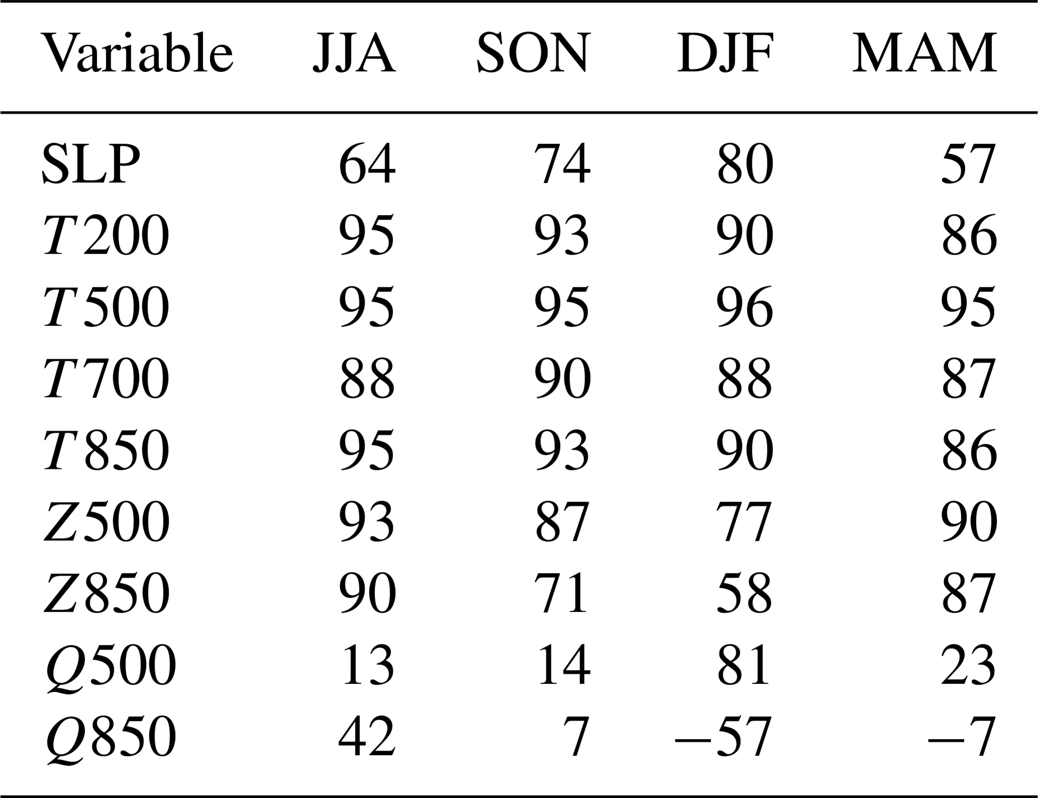
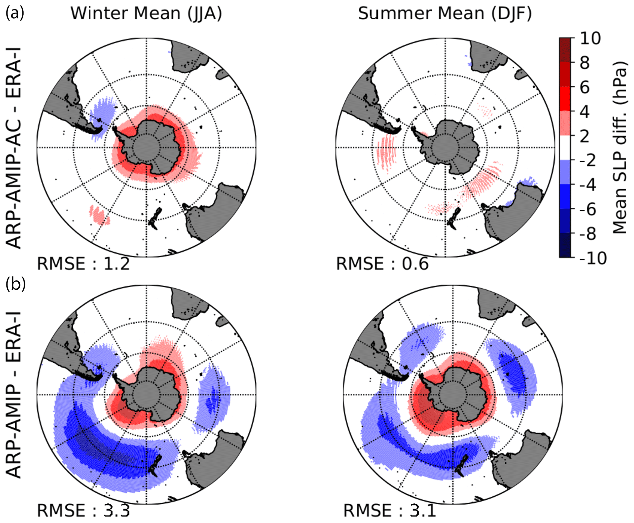
Figure 1Mean SLP difference between ARP-AMIP-AC (a) and ARP-AMIP (b) simulations minus ERA-I for the reference period 1981–2010 in winter (JJA, left) and summer (DJF, right). Value of the RMSE are given below the plots.
Table 3Mean annual 850 hPa westerly maximum strength (WMSTR) and position (WMPOS) in ERA-Interim, ARP-AMIP and ARP-AMIP-AC ± 1 standard deviation of the annual mean. Differences significant at p=0.05 with respect to ERA-I are presented in bold.
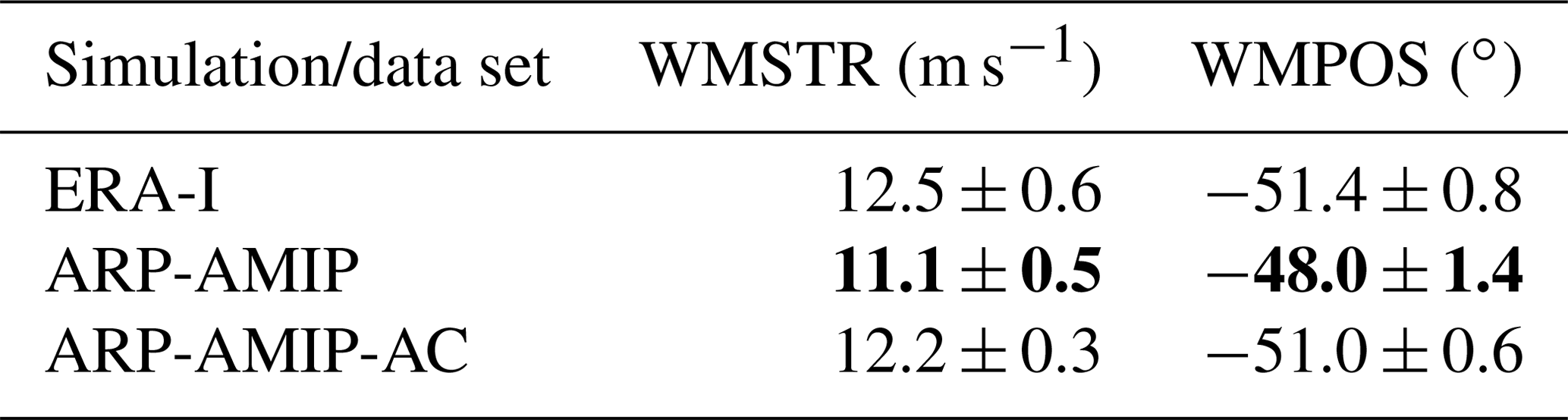
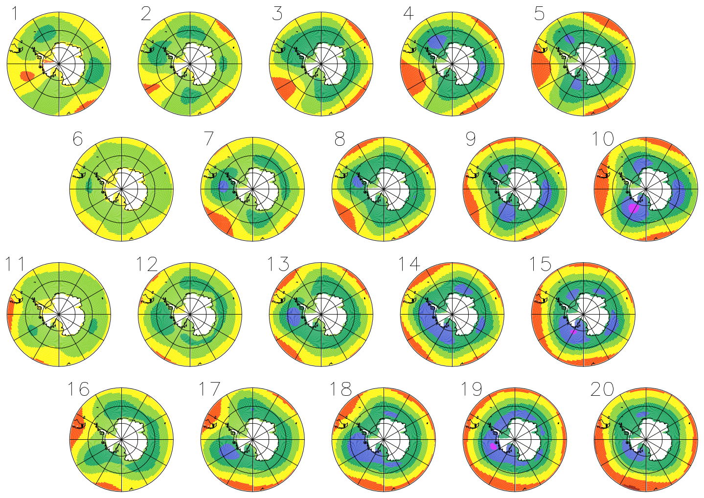
Figure 2Mean sea-level pressure (SLP) map for the 20 best-matching units (BMUs) obtained after a self-organizing map analysis on daily SLP fields. SLP ranges from 1030 hPa (red) to 960 hPa (purple) with 10 hPa intervals.
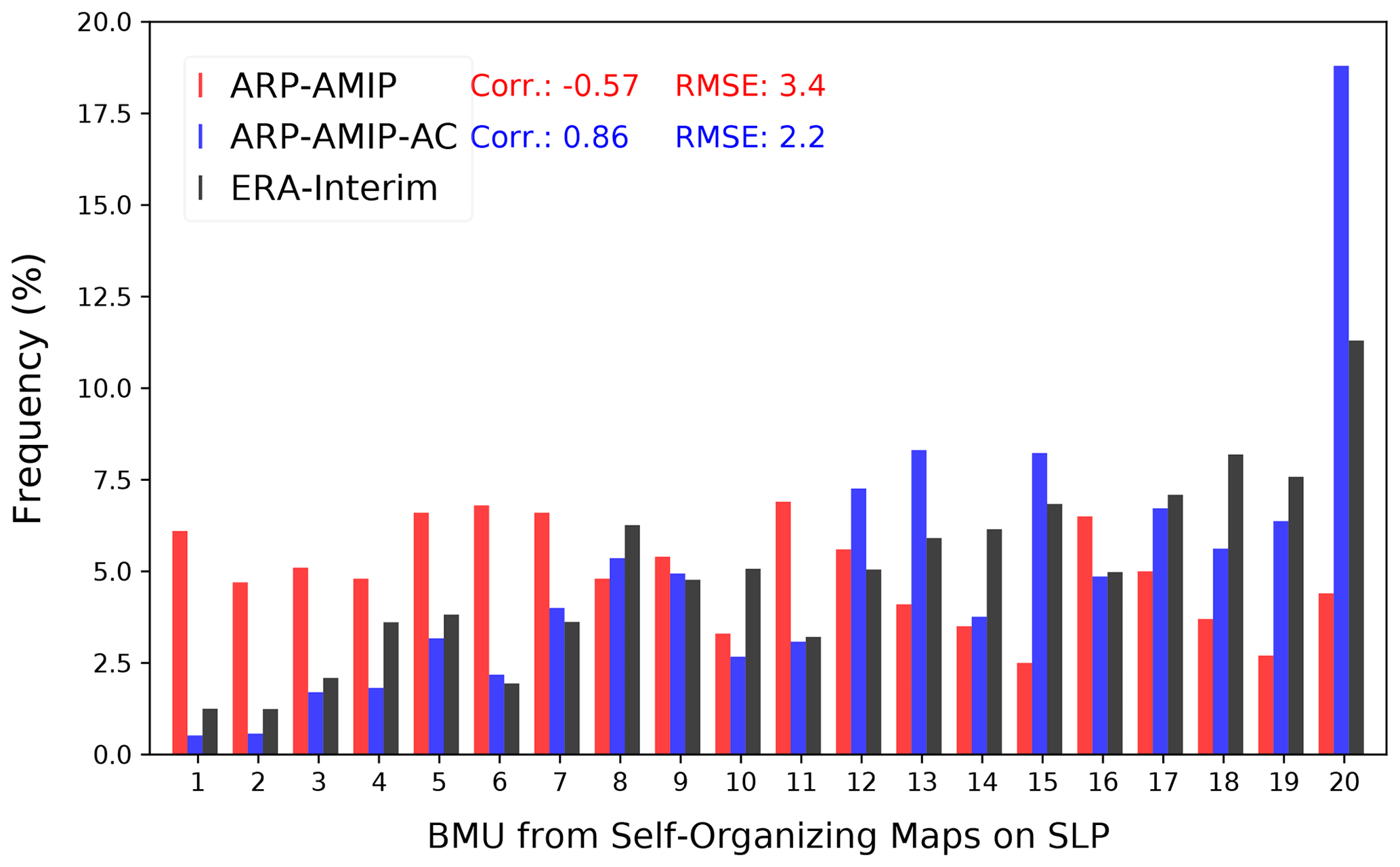
Figure 3Best-matching-unit (BMU) relative frequency (%) of ARP-AMIP (red), ARP-AMIP-AC (blue) and ERA-I (black) on daily SLP map over the 1981–2010 period. Root mean square errors and Pearson correlation coefficient with respect to ERA-I BMU frequencies are shown to the right of the legend.
3.1.3 Near-surface temperatures
The effect of the atmospheric correction on ARPEGE mean near-surface air temperatures (T2 m) can be seen in the ARP-AMIP-AC minus ARP-AMIP difference (Fig. 4a). Here, T2 m values from the corrected ARPEGE simulation are also compared with those from MAR (Agosta et al., 2019) and RACMO2 (van Wessem et al., 2018) RCMs simulations driven at their lateral boundary by ERA-I and those from the weather station of the READER database (Fig. 4b and c). In this analysis, weather stations for which less than 80 % of valid data were available for the season and the period considered have been discarded from the analysis. The same figure for the ARP-AMIP simulation already presented in Beaumet et al. (2019a) can be seen in the Supplement (Fig. S8). The errors for each station and each season, as well as the mean bias for each Antarctic regions for ARP-AMIP-AC and ARP-AMIP, are also presented in the Supplement (Table S4).
On the East Antarctic Plateau (EAP), the impact of the atmospheric bias correction is a winter warming (1–3 ∘C) over large parts of the center of the Plateau. The warm bias with respect to MAR during this season increases, which is confirmed for instance by a decrease in ARPEGE skills at Vostok in all seasons but summer. This bias increase seems to result from the removal of a bias compensation that was present in ARP-AMIP. We investigated the value of the near-surface temperature inversion in both historical ARPEGE simulation (not shown) as the difference between surface temperature (TS) and the temperature of the first atmospheric layer, located around 6 to 10 m height in this ARPEGE setting (level at 0.9988 × surface pressure). The value of this near-surface temperature inversion around (−15 ∘C) does not decrease in ARP-AMIP-AC. It even increases locally, suggesting small changes in surface boundary layer processes. However, there was a substantial negative bias with respect to MAR in incoming long-wave radiation (LWD) in ARP-AMIP, which disappears in ARP-AMIP-AC due to considerable warming at 500 hPa in winter (Fig. S6). The warm bias in winter found over the East Antarctic Plateau with respect to MAR or READER weather stations (between 3 and 5 ∘C), whereas smaller differences are found in the comparison with RACMO2 T2 m), is to be put into perspective with even larger biases sometimes found over the East Antarctic Plateau in climate models or even in climate reanalyses (Dutra et al., 2015; Fréville et al., 2014; Bracegirdle and Marshall, 2012).
For coastal East Antarctic READER stations, the cold bias present in every season, particularly in winter, is greatly reduced in ARP-AMIP-AC. The bias reduction is very large for some stations in eastern East Antarctic (e.g., McMurdo, Dumont D'Urville, Casey, Davis). The effect of the bias correction is also a cooling of some margins of the eastern East Antarctic Plateau in summer, where the warm bias with respect to MAR decreases. However, the errors remain substantial and significant (p<0.05) in many stations and seasons, especially in the winter (mean error ∘C). In this perspective, the comparison with McMurdo and Scott Base is interesting. These stations, distant by only 3 km and located at the same altitude, belong to the same ARPEGE grid point. While ARP-AMIP-AC bias with respect to Scott Base is small and statistically insignificant in all season but summer, the cold bias is ∼ 3 ∘C (significant) throughout the year with respect to McMurdo. This example shows the limited spatial representativity of weather stations in coastal Antarctica, and therefore the comparisons with a 35 km horizontal resolution atmospheric model should be interpreted carefully.
Over West Antarctica and the Peninsula, the effect of the atmospheric bias correction is a warming over much of coastal and central West Antarctica and on the southern and western parts of the Peninsula in winter. In summer, this warming is restricted to the southwestern part of the Peninsula, while there is a cooling of the eastern coasts, particularly marked on the Larsen Ice Shelf. The systematic cold bias with respect to MAR and READER stations of the southern and western part of the Antarctic Peninsula is greatly reduced, with the largest improvements found in the southernmost stations (Rothera and Faraday). Warm and moist advection from the northwest over this part of the Peninsula is indeed underestimated in ARP-AMIP. However, the errors remain significant in summer (mean error ∘C) and in winter for the comparison with RACMO2. Besides, ARP-AMIP-AC is cold biased with respect to MAR over the Larsen Ice Shelf in summer, which was not the case of ARP-AMIP.
No reduction is found for the warm bias on the ice shelves and coastal regions of Dronning Maud Land or for the stations located on the islands of the Southern Ocean where the skill of the AMIP-style control run was already fairly high.
The warm temperature bias with respect to MAR-ERA-I over Antarctic ice shelves does not decrease in ARP-AMIP-AC; it even increases over Neumayer and Halley stations, especially in winter. ARPEGE model deficiencies for surface temperatures over the large Ronne–Filchner and Ross ice shelves have been widely addressed in Beaumet et al. (2019a). They are mostly due to misrepresented stable boundary layer processes and excess (with respect to MAR) in long-wave downward radiation in winter associated with higher cloud cover. Large disagreement have also been evidenced between MAR and RACMO2 for these areas. Indeed, we note that this large winter warm bias is not found over the Ronne–Filchner and is much reduced over the Ross Ice Shelf in the comparison with RACMO2-ERA-I.
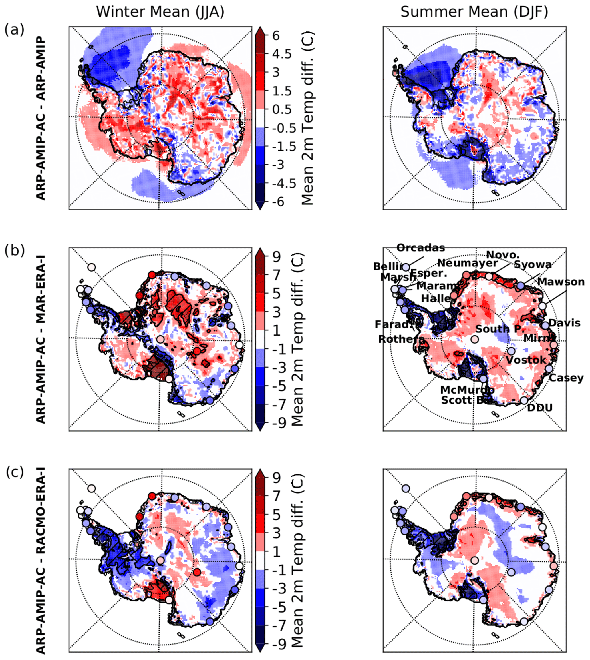
Figure 4(a) ARP-AMIP-AC minus ARP-AMIP T2 m in winter (left) and summer (right). (b) Same as panel (a) but for ARP-AMIP-AC minus MAR-ERA-I. Circles represent mean bias for weather stations from the monthly READER database. Black contour lines represents where the difference is 1 standard deviation of MAR T2 m. (c) Same as panel (b) but for ARP-AMIP-AC minus RACMO2-ERA-I.
3.1.4 Precipitation
Total precipitation integrated over the grounded ice sheet (GIS) for the two ARPEGE simulation over the historical period as well as for MAR and RACMO2 (Agosta et al., 2019; van Wessem et al., 2018) driven by ERA-I reanalysis are shown in Table 4. The spatial distributions of precipitation in ARP-AMIP-AC, ARP-AMIP, MAR-ERA-I and RACMO2-ERA-I are compared in Fig. 5. Precipitation over the GIS significantly decreases in ARP-AMIP-AC with respect to ARP-AMIP (−284 Gt yr−1, ∼ 3 times the inter-annual variability) and is about 10 % lower than the estimates from the two polar RCMs, whereas precipitation in ARP-AMIP is in good agreement with the latter. Unsurprisingly, the precipitation minus evaporation difference (P−E), which is a good approximation of moisture transport, has also decreased in ARP-AMIP-AC (−221 Gt yr−1). The main change in atmospheric general circulation in ARP-AMIP-AC with respect to ARP-AMIP is an increase of SLP at mid-latitude and a decrease around Antarctica, together with a poleward position of the westerly winds maximum, which can be seen as a larger dominance of SAM+-type patterns (see BMU 15, 17, 18, 19 and 20 in Figs. 2 and 3). We note that changes in precipitation in ARP-AMIP-AC with respect to ARP-AMIP (Fig. 5c) bear many similarities with the signature of a positive SAM pattern on Antarctic precipitation assessed in a RACMO2 ERA-Interim-driven simulation in Marshall et al. (2017). It is noteworthy that the link between circulation changes induced by the bias correction and ensuing precipitation changes seen in our simulations is very similar to the effect of bias corrections in the LMDZ model reported by Krinner et al. (2019). It shows mainly a drying in many parts of Antarctica such as Marie Byrd Land, Dronning Maud Land, Victoria Land and the Transantarctic Mountains, a large part of the East Antarctic Plateau up to Adélie Land, and the eastern side of the AP. Conversely, precipitation increases in ARP-AMIP-AC over central and western West Antarctica and over the western side of the Antarctic Peninsula. These changes in precipitation result in a better agreement for the spatial distribution of precipitation with MAR-ERA-I (Fig. 5e and f) over large parts of West Antarctica, Dronning Maud Land and the Peninsula. However, the disagreement between the two model is still considerable (> 20 %) in many places, and the dry bias with respect to MAR-ERA-I present in ARP-AMIP over the East Antarctic Plateau and the Transantarctic Mountains increases. In the comparison of ARPEGE precipitation with those from RACMO2-ERA-I (Fig. 5h and i), the increase in the agreement for ARP-AMIP-AC is much more significant. Many differences between ARP-AMIP with RACMO2 are the same as those seen in the comparison with MAR, and these are also reduced in ARP-AMIP-AC. Moreover, ARP-AMIP-AC and RACMO2 agree remarkably well (errors below 20 %) in many areas with rather complex topography such as Dronning Maud Land, coastal West Antarctica or the Transantarctic Mountains. The systematic dry bias with respect to MAR over the Transantarctic Mountains and Victoria Land is not found in the comparison with RACMO2. This seems to confirm a wet bias in MAR over this area, such as suggested by the comparison with sparse in situ observations evidenced in Agosta et al. (2019).
The widespread dry bias in ARPEGE over the eastern part of the East Antarctic Plateau and the ridges of the western parts of the Plateau is confirmed in the comparison with RACMO2 and explains most of the ∼ 10 % precipitation deficit at the continental scale in the ARP-AMIP-AC simulation with respect to both RCMs. Further investigations are needed in order to identify possible causes of this error, such as deficiencies in moisture transport over the high continental interior or misrepresented clear-sky precipitation processes, which bring a large share of total precipitation in this area (Walden et al., 2003). Improvement for the representation of precipitation, cloudiness and therefore radiative budget for the high continent interior of Antarctica could be obtained for ARPEGE by accounting for saturation with respect to the ice for the formation of cloud condensates and by tuning cloud microphysics to the cold context of Antarctica such as done in van Wessem et al. (2014).
The better agreement (decrease in RMSE) with precipitation modeled by the polar-oriented RCMs MAR and RACMO2 precipitation increases the confidence in the reliability of spatial distribution of Antarctic precipitation modeled in ARP-AMIP-AC. Both RCMs have been widely validated against in situ measurements of Antarctic SMB (e.g., Agosta et al., 2019; van Wessem et al., 2018). The closer agreement between the ARP-AMIP-AC simulation and RACMO2 in coastal areas offers an interesting opportunity to further investigate causes of remaining disagreement between MAR and RACMO2 in Antarctic precipitation and SMB identified in Agosta et al. (2019). In this paper, it is argued that RACMO2 does not account for horizontal transport of falling precipitation and therefore misses some of the sublimation of snowfall in the dry katabatic layer such as shown in Grazioli et al. (2017). The same issue could be present in ARPEGE simulations due to the relatively large model physics time step used (15 min).
3.1.5 Surface mass balance
The SMB and its components integrated over the whole grounded ice sheet (GIS) for the 1981–2010 reference period are also presented in Table 4 for the two historical ARPEGE simulations and for ERA-I-driven MAR and RACMO2 simulations. The spatial distribution of SMB for the different model and associated differences can be seen in Fig. 6. The same figure for surface sublimation is shown in the Supplement (Fig. E1). The difference in GIS SMB in ARP-AMIP-AC with respect to MAR-ERA-I and RACMO2-ERA-I is about 4 times the GIS SMB inter-annual variability (σ) of the latter as a consequence of lower precipitation and largely overestimated surface sublimation rates (and, to a lesser extent, runoff). In the atmosphere-corrected simulation, there is a significant decrease in runoff and surface snow sublimation with respect to previously uncorrected simulation yet insufficient to match with the estimates from the two polar-oriented RCMs. The overestimation is still large for the comparison with RACMO2 simulation where sublimation includes surface and blowing snow sublimation (see Table 4). The overestimation of surface sublimation in ARPEGE is consistent with the warm bias evidenced previously in winter over the Antarctic Plateau and in summer at the fringe of the Plateau (see Fig. 4). The model deficiencies in capturing the frequent formation of very stable boundary layer in Antarctica are indeed expected to cause an overestimation of turbulent mixing and heat fluxes near the surface. These biases are also consistent with an overestimation of surface runoff and snowmelt in summer. Estimations of surface snowmelt in ARP-AMIP-AC are nevertheless within the 1σ uncertainty range when compared to RACMO2 and MAR.
Vaughan et al. (1999)Table 4Mean GIS surface mass balance and its components (Gt yr−1) ± 1 standard deviation of the annual value for the reference period 1981–2010. ARPEGE values are integrated over the original model grid and take into account the model land mask. ARPEGE, 1 MAR and RACMO2 ERA-Interim-driven statistics for 1981–2010 for the Antarctic GIS using MAR grounded ice masks (GIS area = 12.37 × 10⁶ km2). 2 RACMO2 original data source is van Wessem et al. (2018). Statistics in bold for ARP-AMIP-AC are statistically different from ARP-AMIP at p=0.05.
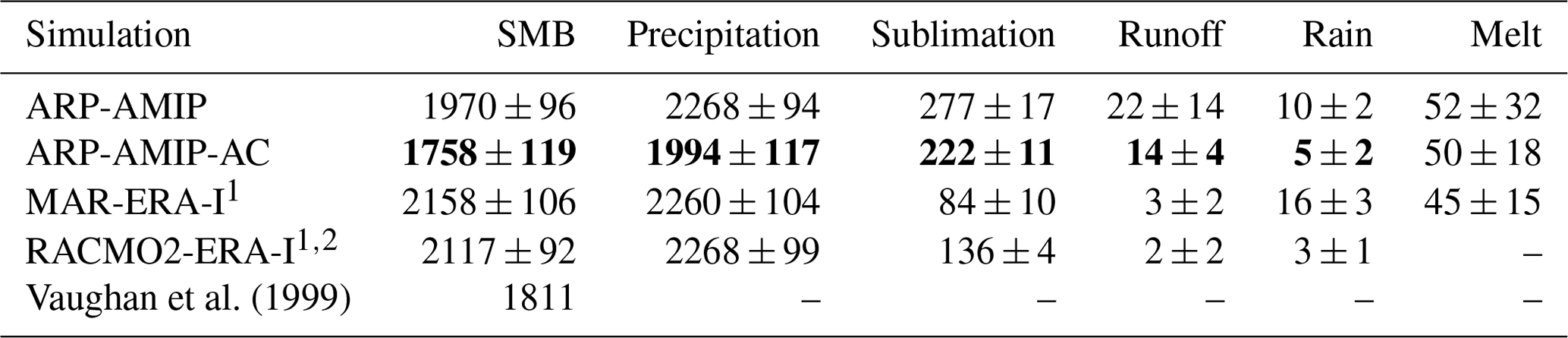
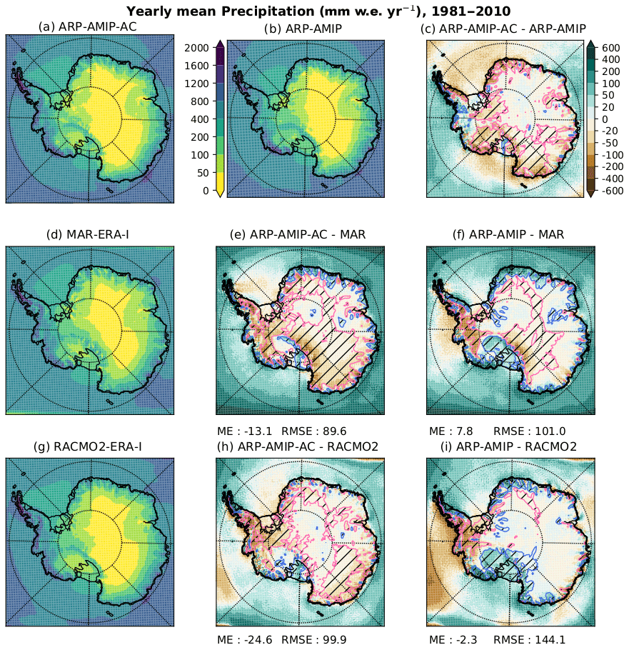
Figure 5Yearly mean total precipitation (mm w.e. yr−1) for ARP-AMIP-AC (a), ARP-AMIP (b), MAR-ERA-I (d) and RACMO2-ERA-I (g) for the reference period 1981–2010. Difference (mm w.e. yr−1) for ARP-AMIP-AC minus ARP-AMIP (c), ARP-AMIP-AC minus MAR-ERA-I (e), ARP-AMIP minus MAR-ERA-I (f), ARP-AMIP-AC minus RACMO2-ERA-I (h) and ARP-AMIP minus RACMO2-ERA-I (i). Blue (magenta) hatched contour lines represent areas where the positive (negative) difference is larger than 20 %. Mean error (ME) and RMSE statistics (mm w.e. yr−1) for the comparison with MAR and RACMO2 are shown below the panel.
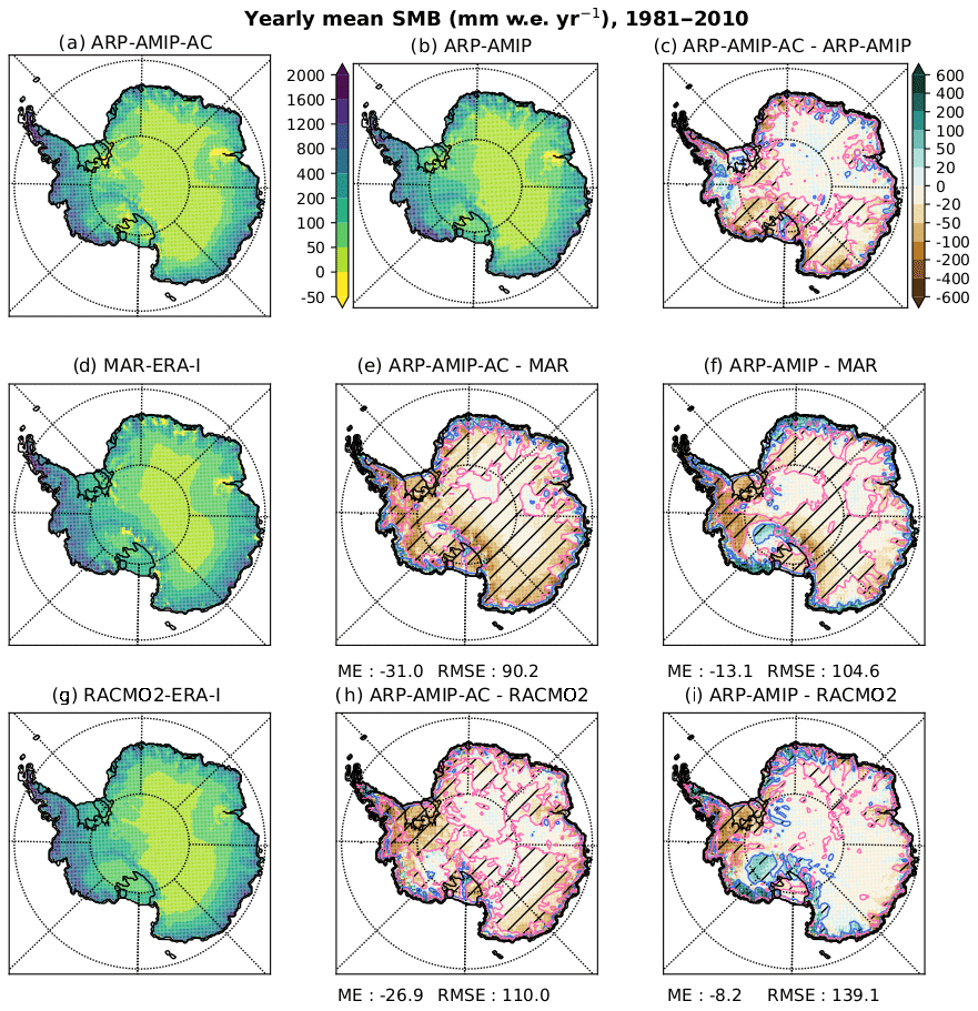
Figure 6Yearly mean total SMB (mm w.e. yr−1) for ARP-AMIP-AC (a), ARP-AMIP (b), MAR-ERA-I (d) and RACMO2-ERA-I (g) for the reference period 1981–2010. Difference (mm w.e. yr−1) for ARP-AMIP-AC minus ARP-AMIP (c), ARP-AMIP-AC minus MAR-ERA-I (e), ARP-AMIP minus MAR-ERA-I (f), ARP-AMIP-AC minus RACMO2-ERA-I (h) and ARP-AMIP minus RACMO2-ERA-I (i). Blue (magenta) hatched contour lines represent areas where the positive (negative) difference is larger than 20 %. Mean error (ME) and RMSE statistics (mm w.e. yr−1) for the comparison with MAR and RACMO2 are shown below the panel.
3.2 Climate change signal
In this section, we present and compare the climate change signals for late 21st century obtained in the different ARPEGE RCP8.5 projections presented in this study. Climate change signals are obtained by computing the difference with their reference simulation in present-day climate (see Table 1). Differences in changes in atmospheric general circulation, near-surface temperature, precipitation and SMB obtained when using atmospheric bias correction and their consistency with previous studies are more specifically emphasized and discussed.
3.2.1 Atmospheric general circulation
Changes in atmospheric general circulation are summarized by representing the Southern Hemisphere latitudinal profiles of sea-level pressure for each of the present-day simulation and future projections (Fig. 7). The simulated climate change signal is represented by the difference between each projection (colored lines) and their reference simulation for present-day climate (dashed or plain lines). It can be seen that each future projection is characterized by a strengthening of the mid-latitude highs and a deepening of the circum-Antarctic troughs and by a poleward movement of these features with respect to their reference historical simulation. This corresponds to an increasingly positive phase of the Southern Annular Mode (SAM) index, the main mode of variability of atmospheric general circulation in the southern high latitudes, which is in good agreement with the generally expected consequences of the increase in GHG concentration on the Southern Hemisphere's high-latitude atmospheric circulation for the late 21st century (Arblaster and Meehl, 2006; Miller et al., 2006; Fyfe and Saenko, 2006).
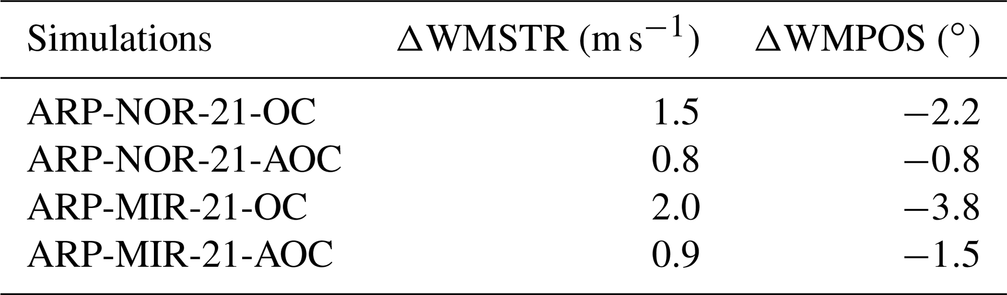
However, it is noteworthy that both projections realized with atmospheric bias corrections show substantially weaker changes in this increase of the meridional surface pressure gradient as well as a weaker poleward shift. This is confirmed by statistics from the changes in 850 hPa westerly maximum strength and position (ΔWMPOS and ΔWMSTR, Table 5). Each future projection (bias-corrected or not) displays a strengthening and poleward movement of the westerly maximum, but the magnitude of these climate change signals is about 50 % smaller in ARPEGE bias-corrected projections with respect to the non-corrected control run. In similar experiments conducted with the LMDZ model (Krinner et al., 2019) with different oceanic forcings, similar results were found. The magnitude of this difference is however much more reduced when compared to the results with ARPEGE. The realism of this reduced poleward shift and strengthening is discussed more extensively in Sect. 4.1 and in the Supplement. Future projections realized with MIROC-ESM SSCs (higher decrease in sea ice) show a larger southward displacement of the westerlies than the one realized with NorESM1-M SSCs, which is consistent with the impact of sea-ice extent on the position of the westerly winds maximum evidenced in previous studies (Krinner et al., 2014; Bracegirdle et al., 2018).
Another main difference in projected changes in atmospheric general circulation is the largely reduced deepening (not shown) of the Amundsen Sea Low (ASL), the main pressure climatological minimum, which is located at the fringe of the Amundsen and the Ross Sea in winter and off the Bellingshausen Sea, west of the Antarctic Peninsula in summer (Raphael et al., 2016). Blocking activity in the Amundsen Sea region and a negative phase of the SAM, which both correlate with El Niño conditions (Scott Yiu and Maycock, 2019), have been found to influence warming rates in West Antarctica (Scott et al., 2019). Since the SAM pattern and the deepening of the ASL were found to be different in ARPEGE bias-corrected projections, this will likely impact blocking activity in the Amundsen Sea region and therefore warming in West Antarctica. A detailed analysis in our ARPEGE simulation of this relationship between regional warming and blocking activity associated with the propagation of Rossby waves in the Pacific sector is however beyond the scope of this study.

Figure 7Yearly mean sea-level pressure (hPa) for ARPEGE historical simulation (1981–2010) and RCP8.5 projections (2071–2100). Uncorrected control runs are displayed in dashed lines and runs with atmospheric bias correction are presented in plain lines. Historical simulations realized with observed SSCs are displayed in black (ARP-AMIP-AC) or gray (AMIP). Future projections (RCP8.5) driven by bias-corrected SSCs from NorESM1-M (MIROC-ESM) are shown in red (green).
Table 5Anomalies in southern westerlies maximum strength (ΔWMSTR, m s−1) and position (ΔWMPOS, ∘) for the different ARPEGE projections.
3.2.2 Near-surface temperature
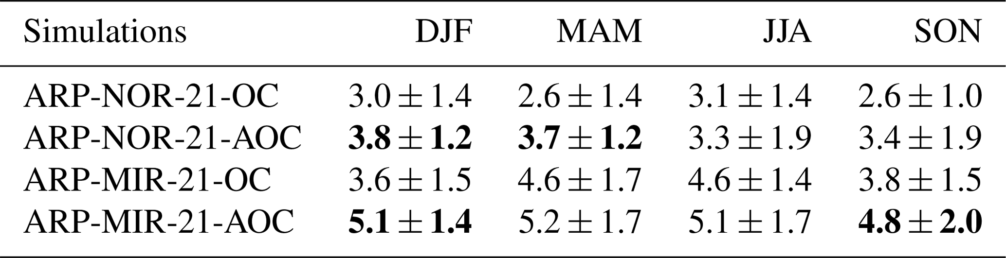
The increases in mean yearly T2 m averaged over the GIS are respectively 3.5 ± 1.0 and 5.0 ± 1.3 ∘C for ARP-NOR-21-AOC and ARP-MIR-21-AOC. This represents respectively a +0.7 and +0.9 ∘C additional warming (significant at p<0.05) compared to the corresponding projections without atmospheric bias correction. Differences in warming rate per season are presented in Table 6. Differences in warming for the atmospheric-corrected simulations are the largest in summer and are significant for both projections, while they are smaller and not significant in winter. For ARP-NOR-21-AOC, the larger warming in autumn (MAM) is also significant, and so it is in spring for ARP-MIR-21-AOC.
The spatial distribution of the increase in T2 m and corresponding differences in winter (JJA) and summer (DJF) warming are presented in Fig. 8. The two sets of projections show very similar patterns in terms of differences in regional warming. The larger surface warming in summer in the atmospheric-corrected experiment is essentially the consequence of a stronger temperature increase over East Antarctica. This larger additional warming found for the surface of the East Antarctic Plateau in summer (+1 to +2 ∘C) is also found at higher altitudes (500 hPa), which results in increased LWD. This additional warming is consistent with the weaker increase of the pressure gradient and a reduced poleward shift of the westerly winds in these projections, as this corresponds to a lower increase towards a more positive phase of the SAM in future climate. The link between negative (positive) anomalies of the SAM and positive (negative) temperatures anomalies over the East Antarctic Plateau has been established in many previous studies (e.g., Marshall and Thompson, 2016; Kwok and Comiso, 2002) and was found to be stronger in summer and autumn (Marshall, 2007; Clem et al., 2016). However, following this hypothesis and the findings from Marshall and Thompson (2016), less pronounced positive phase of the SAM should also result in a larger warming over West Antarctica and a weaker warming over the northeastern Peninsula in atmosphere-corrected projections, which is not the case here.
In winter, there is a well-marked dipole with lower warming over West Antarctica and the Ross Ice Shelf and higher warming over southern Victoria and Adélie Land. The much weaker deepening of the Amundsen Sea Low found in our atmosphere-corrected experiments is consistent with these differences in regional warming. The mean position of the Amundsen Sea Low was indeed shown to be located over the east side of the Ross Sea in winter (Raphael et al., 2016), and so it is in ARPEGE simulations.
Systematically, near-surface temperature increases are the strongest where sea ice is lost. This is particularly noticeable over the northern part of the Weddell Sea. This area (together with Larsen and Ronne–Filchner ice shelves) shows a large additional warming in atmosphere-corrected experiments.
Overall, most of the differences in near-surface temperatures warming found are consistent with corresponding differences in large-scale atmospheric circulation changes and the relation found between pressure and temperature anomalies in previous studies.

Figure 8T2 m anomaly for ARPEGE RCP8.5 projection for the late 21st century (reference period: 1981–2010) with atmospheric bias correction (AOC, left), uncorrected atmosphere (OC, center) and difference (right). Anomalies for winter (JJA) are displayed at the top of the subfigures and for summer (DJF) at the bottom. Results for projections with bias-corrected SSCs from NorESM1-M (respectively MIROC-ESM) are shown in panel (a) (respectively b). Gray contour lines show where differences in anomaly are >25 % with respect to the uncorrected control run.
Table 6Mean seasonal T2 m increase (K) for the Antarctic GIS for the different ARPEGE RCP8.5 projection for the late 21st century with respect to their historical reference simulation. Anomalies in projections with bias-corrected atmosphere significantly different (p<0.05) from the anomaly in the uncorrected control run level are shown in bold.
3.2.3 Precipitation and surface mass balance
Absolute and relative increase in SMB and for its different components for the Antarctic GIS are presented in Table 7. All projections show an increase in surface mass balance, resulting from the absolute increase in precipitation still being much larger than the corresponding increases in surface sublimation and runoff. This is in agreement with previous Antarctic climate change studies for the late 21st century (e.g., Lenaerts et al., 2016; Krinner et al., 2014; Frieler et al., 2015). Additional increases in total precipitation of +78 and +90 Gt yr−1, which corresponds respectively to a +6 and +9 % additional relative increase (not significant at p<0.05), are found respectively for ARP-NOR-21-AOC and ARP-MIR-21-AOC atmospheric-corrected projections. In ARP-MIR-21-AOC, a significant higher increase in surface sublimation mitigates slightly the increase in SMB with respect to ARP-MIR-21-OC. Despite a larger warming at the continental scale, increases and cumulated amounts of precipitation are significantly lower in projections with atmospheric bias correction. There is an additional increase in moisture transport towards the AIS (approximated through P−E) of +3.5 and +5.8 % respectively with respect to uncorrected control run. The sensitivity to temperature of the increase in precipitation (α) in ARP-NOR-21-AOC and ARP-MIR-21-AOC is respectively +7.7 % K−1 and +9.1 % K−1, whereas it was respectively +5.2 % and +8.8 % in the uncorrected control run. This suggests that a significant part of the additional increase in precipitation is due to different changes in the atmospheric general circulation, particularly in the projection driven by NorESM1-M oceanic boundary conditions, while a remaining part is of course due to increased moisture-holding capacity of the atmosphere due to higher warming. The latest values found for α are somewhat higher than previous estimates (Krinner et al., 2008; Frieler et al., 2015; Ligtenberg et al., 2013; Palerme et al., 2017), which usually range between +5 and +7 % K−1. However, Bracegirdle et al. (2015) also evidenced that α tends to be higher in models projecting a larger decrease in sea-ice extent, which is the case for experiments forced by MIROC-ESM sea-ice anomaly.
The spatial distribution of precipitation changes for each projection are shown in Fig. 9 along with the differences between the corrected simulations and the uncorrected control runs. Projections with atmospheric bias correction show a smaller precipitation increase over most of West Antarctica, the Transantarctic Mountains and western Dronning Maud Land. Conversely, the increase in precipitation is larger on the coastal AP, on the Ross side of Marie Byrd Land and on Adélie and southern Victoria Land, where uncorrected projections suggest a precipitation decrease. The higher precipitation increase over Adélie and southern Victoria Land and the corresponding weaker increase over most of West Antarctica can be related, as for the corresponding dipole in differences of warming in winter, to the weaker deepening to the Amundsen Sea Low in bias-corrected projections. Winter is indeed, with autumn, the season of highest precipitation rates over peripheral Antarctica (Palerme et al., 2017).
Additionally, Palerme et al. (2017) found that CMIP5 models which agree better with Antarctic snowfall derived from CloudSat show a larger warming (+0.4 ∘C) and a higher precipitation increase (+4.8 %) with respect to the ensemble mean in their RCP8.5 projections. In light of our results, it would be interesting to investigate whether models agreeing with CloudSat snowfall are doing so because of a better representation of the atmospheric general circulation and whether the higher increase in temperature and precipitation can be generally linked to the better representation of atmospheric general circulation in the context of CMIP ensembles such as found in our bias-corrected experiment.
Table 7Absolute values and absolute (Abs.) and relative (Rel.) anomalies for mean SMB and its components (Gt yr−1) for the Antarctic GIS in the different ARPEGE RCP8.5 projections (reference period: 1981–2019). Anomalies and absolute values significantly different (p<0.05) in projections realized with bias-corrected atmosphere with respect to control run are displayed in bold.
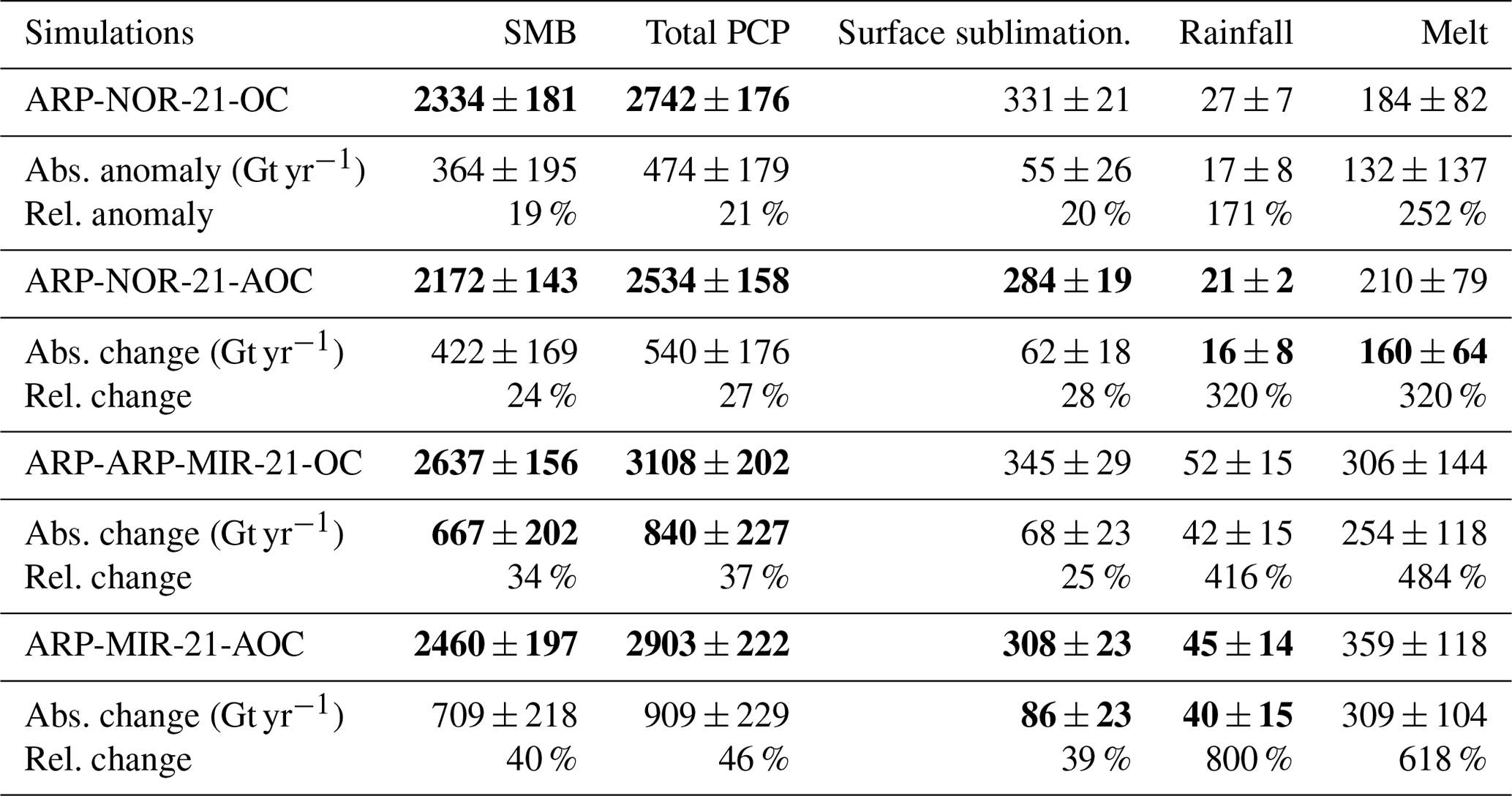
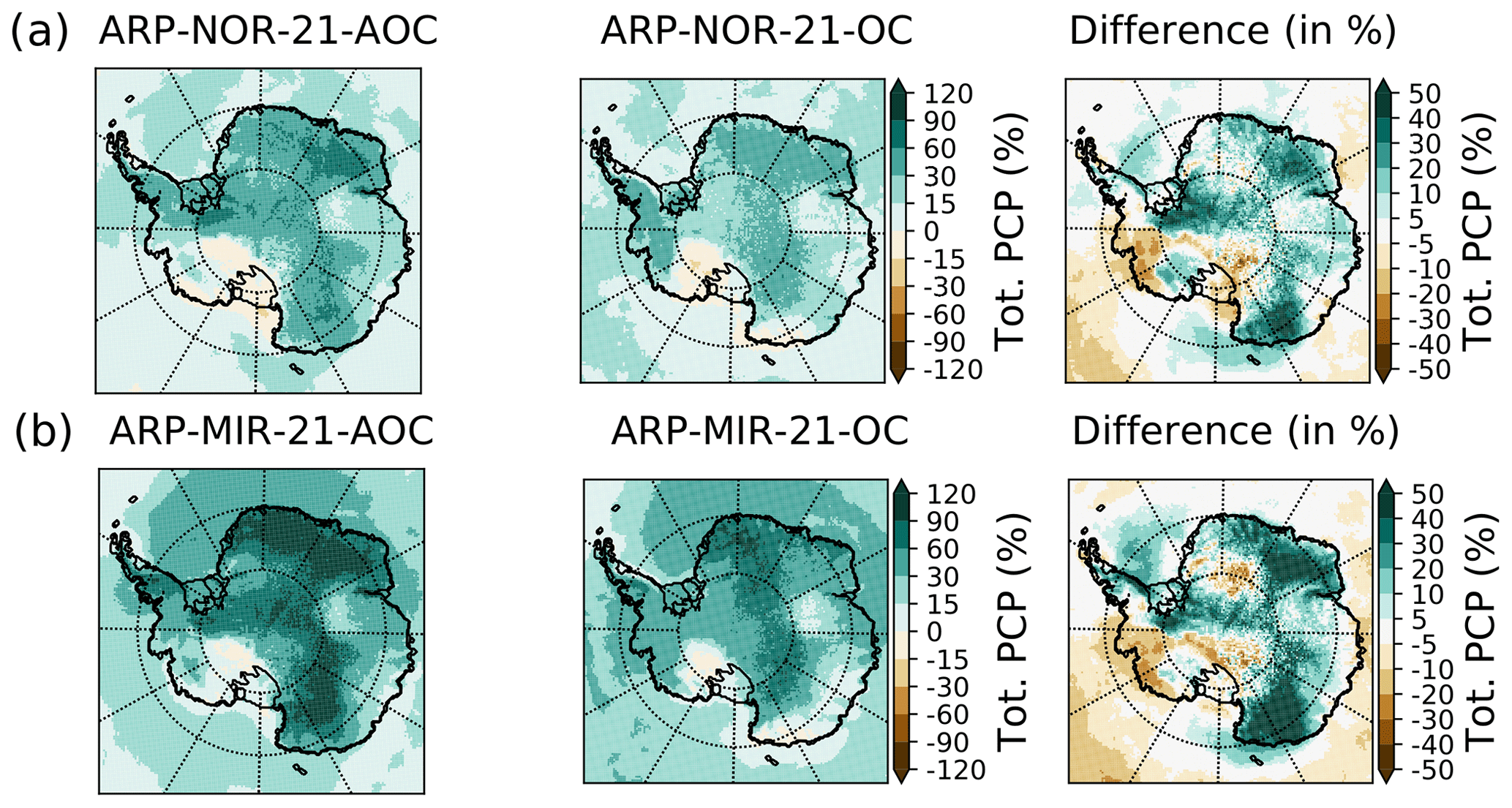
Figure 9Late 21st century anomalies in yearly total precipitation (%) for ARPEGE RCP8.5 projections with atmospheric bias correction (left), uncorrected reference simulation (center) and difference (right). Results for projections with bias-corrected SSCs from NorESM1-M (respectively MIROC-ESM) are presented in panel (a) (respectively b).
In this section, we discuss the realism of projected climate change in bias-corrected projections as well as the future perspectives associated with the method and the results presented in this study.
4.1 Realism of projected changes
In future works, the remaining uncertainties on the less pronounced strengthening of the pressure gradient and the large magnitude of the reduced poleward shift found in atmospheric bias-corrected experiments should be reduced with additional experiments using either another set oceanic surface forcing or other atmospheric models, considering the large impacts of these on the projected climate change for the Southern Hemisphere high latitudes. These results are however consistent with results from Barnes and Hartmann (2012), who found, using GCMs future projections and an idealized-case barotropic model, that there is a theoretical limit to how far south the maximum of cyclonic wave breaking can move as these dynamical changes are constrained by the absolute vorticity gradient. Their results suggested that the currently observed Southern Hemisphere general circulation might already be close to this limit. Investigating these same physical mechanisms such as done in Barnes and Hartmann (2012) in our ARPEGE bias-corrected experiments is out of the scope of this study, and generalizing results from a set of only two pairs of 30-year experiments would be impossible due to the climate's internal variability. Nevertheless, when we put them in the context of previous CMIP5 large ensemble analyses (Bracegirdle et al., 2013), we confirm that these processes are likely at play in our simulations (Fig. S4).
Even though the realism of projected changes in bias-corrected experiments still and will always bear uncertainties (as by construction future climate projections are impossible to verify), the uncorrected projections are expected to be of limited use for impact assessment studies since biases in the historical reference experiment are of the same order of magnitude as projected changes. In such impact assessment studies, the absolute future state of the climate is more relevant than relative projected changes. An interesting example is given with the impact of the position and depth of the Amundsen Sea Low on the regional changes in temperature and precipitation over western West Antarctica, Victoria and Adélie Land. While the more reliable deepening and displacement of the ASL in the bias-corrected projections with respect to non-corrected reference can still to some extent be questioned, the impact of this deepening and displacement on regional temperature and precipitation changes are by construction more realistic in the bias-corrected projections as the biased position and depth of the ASL in the historical uncorrected simulation already induce incorrect regional temperature and precipitation patterns for present time. Assessing the impact of extreme events in a changing climate using projections that have a highly biased representation of the Antarctic's climate mean state and variability in their historical reference is unrealistic. In our study, we found that the climate's variability at the daily timescale is better represented in ARPEGE bias-corrected experiment. This is an important result as by construction the empirical bias correction is expected to reduce biases on mean state only. Krinner et al. (2019, 2020) found similar results in their application with LMDZ and other atmospheric models for the representation of climate variability ranging from daily to inter-decadal timescales. This is another argument in favor of using bias-corrected projections for impact assessment studies as a better representation of the climate variability is expected to bring more useful information on extreme events.
4.2 Implication and perspectives
The large bias reductions for large-scale atmospheric circulation and surface climate obtained in this study should not be perceived as an argument against pursuing the efforts to improve the dynamics and physics of coupled and atmospheric models in a physically consistent and comprehensive way nor as a loss of confidence in these tools. These are crucial in order to explore some feedbacks and interactions between the different component of the Earth system in a warming climate. Yet, as long as biases of state-of-the-art climate models are of about the same order of magnitude as projected changes at the end of current century (Flato et al., 2013), a posteriori statistical bias correction (Hall, 2014; Maraun and Widmann, 2018) will be applied to future projections before they are used as input for impact assessment studies. However, these methods fail to correct for biases due to atmospheric circulation errors (Eden et al., 2012; Stocker et al., 2015; Maraun et al., 2017). Therefore, the method presented in this study offers an excellent opportunity to circumvent this drawback. Bias stationarity is a strong hypothesis needed to support the application of run-time atmospheric bias correction in climate projections. However, the evidence of large stationarity in biases of coupled models on large-scale atmospheric circulation evidenced in Krinner and Flanner (2018) and the preservation of the added value of the value until late 21st century climate evidenced in Krinner et al. (2020) using the perfect model test framework supports this application under strong climate change.
Bias correction can be easily turned off, and its impact on projected climate change can easily be identified. Therefore, applying these bias-correction methods also allows us to assess remaining uncertainties on projected climate change in coupled and atmospheric climate models such as suggested by Dommenget and Rezny (2018) and could help in identifying which efforts one should focus on in order to reduce these uncertainties. Considering it removes most of the biases on large-scale atmospheric circulation, the bias-correction method implemented in this study also offers the opportunity to test the tuning of the parametrizations of smaller-scale processes (e.g., boundary layer) in a different context (freely evolving simulation) than nudged simulations often used in this purpose. This would allow us to test whether introduced modifications in new parametrizations are detrimental to the model skills on large-scale atmospheric circulation when the model is not constrained by atmospheric reanalysis.
Even though they still bear some uncertainties, the significant differences in large-scale atmospheric circulation and surface climate changes reported in this study could have large impacts on projected changes of the Antarctic ice-sheet mass balance. Therefore, we suggest to use surface forcing provided by our bias-corrected projections to drive ice dynamics or ocean and ice shelf interaction studies. Downscaling the projections presented in this study with polar-oriented RCMs such as MAR and RACMO2 could also help to identify remaining uncertainties associated with ARPEGE biases on Antarctic surface climate and SMB mostly associated with its less sophisticated surface snow scheme, and these new downscaled projections would help better constrain future ice dynamics or ice–ocean–atmosphere interactions.
In this study, we used empirical run-time bias correction following the method described in Guldberg et al. (2005) or in Kharin and Scinocca (2012). In order to build correction terms, we used the climatology of the adjustment term on tendency errors coming from an ERA-Interim-driven ARPEGE simulation over the 1993–2010 period. In this experiment, nudged variables were air temperature, air specific humidity, logarithm of surface pressure, divergence and vorticity with a relaxation time of 72 h.
The application of this method over present climate (1981–2010) yielded a substantial bias reduction in the representation of large-scale atmospheric circulation in the Southern Hemisphere. The biases of westerly wind maximum position and strength were almost completely suppressed. This improvement of southern hemispheric general circulation produced a decrease of the biases on near-surface temperature over the Antarctic Peninsula, while we found a slightly increased warm winter bias on the East Antarctic Plateau. Regarding precipitation, the agreement with polar-oriented RCMs MAR and RACMO2 has increased, especially in the comparison with the latter, where differences below 20 % are reported over most coastal areas. A dry bias in the atmosphere-corrected experiment over the summit of the East Antarctic Plateau was also evidenced by this comparison with polar-oriented RCMs.
The application of the method for future climate projections (RCP8.5) using bias-corrected oceanic forcing from MIROC-ESM and NorESM1-M has revealed considerable differences in projected changes in large-scale atmospheric circulation. The strengthening and the poleward shift of the westerly wind maximum are reduced by about 50 % with respect to uncorrected reference projections. These differences in change of atmospheric general circulation have caused significant additional warming of +0.7 to 0.9 K, resulting essentially from the much larger warming of East Antarctica in summer. A dipole with higher warming and increase in precipitation over southern Victoria and Adélie Land and corresponding lower warming and increase in precipitation over most of West Antarctica is also found in winter. This is attributed to a reduced deepening of the Amundsen Sea Low in the atmosphere-corrected projections.
The magnitude of the difference in changes of large-scale atmospheric circulation needs to be confirmed with experiments using other oceanic forcing or other atmospheric models, as these would have large impacts on the evolution of the Antarctic ice-sheet mass balance. However, a reduced poleward shift of the westerlies maximum in the bias-corrected experiments is consistent with the state dependence on historical biases in CMIP5 projections evidenced in previous studies. Many of the differences found in projected changes in temperature and precipitation are also consistent with previously evidenced signatures of pressure anomalies, especially considering a weaker SAM+ anomaly.
Because statistical bias corrections, usually applied to climate model output before their use for impact studies, generally fail to correct biases associated with errors on atmospheric general circulation, the method proposed in this study offers interesting perspectives. The downscaling of atmosphere-corrected projections with polar-oriented RCMs could help to better constrain the evolution of the future Antarctic ice-sheet surface mass balance and evaluate remaining uncertainties in this study associated with ARPEGE biases on surface climate. The potentially large effect on the Antarctic ice sheet of the differences in snow accumulation and surface climate changes suggested in this study should be explored using surface forcings coming from atmosphere-corrected projections to drive ice dynamics or ocean and ice shelf interaction impact studies.
Historical run and future projections presented in this study are available on the Antarctic CORDEX grid at a daily time step for atmospheric surface temperature (mean, min and max), precipitation, snowfall, surface snowmelt, surface runoff and surface snow sublimation at the following address: https://doi.org/10.5281/zenodo.4059193 (Beaumet et al., 2020). Data and metadata mostly follow CORDEX recommendations. Atmospheric variables (temperature, wind specific humidity, geopotential and surface pressure) over 17 constant-pressure levels at a 6-hourly resolution are available for the Southern Hemisphere upon request.
The supplement related to this article is available online at: https://doi.org/10.5194/tc-15-3615-2021-supplement.
AA prepared the ARPEGE version and scripts that were used to produce the ARPEGE runs used in this study. MD performed the sensitivity tests and ran the bias-corrected simulations. JB ran the non-corrected reference runs, analyzed the output, and prepared the manuscript and the figures. CA provided MAR outputs and useful scripts for the interpolation and comparisons of MAR, RACMO2 and ARPEGE output. GK read and corrected the manuscript many times. All the authors have provided complete reviews and relevant remarks for the improvement of the manuscript.
The authors declare that they have no conflict of interest.
Publisher's note: Copernicus Publications remains neutral with regard to jurisdictional claims in published maps and institutional affiliations.
We acknowledge the World Climate Research Programme's Working Group on Coupled Modelling, which is responsible for CMIP, and we thank the climate modeling groups participating in CMIP5 for producing and making available their model output. For CMIP the U.S. Department of Energy's Program for Climate Model Diagnosis and Intercomparison provided coordinating support and led development of software infrastructure in partnership with the Global Organization for Earth System Science Portals.
The Centre National de Recherches Météorologiques (Météo-France, CNRS) and associated colleagues are warmly thanked for providing resources and help to run ARPEGE model.
We also thank the Scientific Committee on Antarctic Research (SCAR) and the British Antarctic Survey for the availability of the SCAR READER database.
We kindly acknowledge Michiel van den Broeke for providing RACMO2 data and helpful discussions.
Finally, we want to thank the two anonymous reviewers for their constructive remarks and the editor for helping in improving the quality of this paper.
This publication was supported by PROTECT. This project has received funding from the European Union’s Horizon 2020 research and innovation program under grant agreement no. 869304. This is PROTECT contribution number 21.
This paper was edited by Masashi Niwano and reviewed by two anonymous referees.
Agosta, C., Favier, V., Krinner, G., Gallée, H., Fettweis, X., and Genthon, C.: High-resolution modelling of the Antarctic surface mass balance, application for the twentieth, twenty first and twenty second centuries, Clima. Dynam., 41, 3247–3260, https://doi.org/10.1007/s00382-013-1903-9, 2013. a
Agosta, C., Amory, C., Kittel, C., Orsi, A., Favier, V., Gallée, H., van den Broeke, M. R., Lenaerts, J. T. M., van Wessem, J. M., van de Berg, W. J., and Fettweis, X.: Estimation of the Antarctic surface mass balance using the regional climate model MAR (1979–2015) and identification of dominant processes, The Cryosphere, 13, 281–296, https://doi.org/10.5194/tc-13-281-2019, 2019. a, b, c, d, e, f, g, h
Arblaster, J. M. and Meehl, G. A.: Contributions of External Forcings to Southern Annular Mode Trends, J. Climate, 19, 2896–2905, https://doi.org/10.1175/JCLI3774.1, 2006. a, b
Barnes, E. A. and Hartmann, D. L.: Detection of Rossby wave breaking and its response to shifts of the midlatitude jet with climate change, J. Geophys. Res.-Atmos., 117, D09117, https://doi.org/10.1029/2012JD017469, 2012. a, b
Beaumet, J., Déqué, M., Krinner, G., Agosta, C., and Alias, A.: Effect of prescribed sea surface conditions on the modern and future Antarctic surface climate simulated by the ARPEGE atmosphere general circulation model, The Cryosphere, 13, 3023–3043, https://doi.org/10.5194/tc-13-3023-2019, 2019a. a, b, c, d, e, f, g, h, i, j
Beaumet, J., Krinner, G., Déqué, M., Haarsma, R., and Li, L.: Assessing bias corrections of oceanic surface conditions for atmospheric models, Geosci. Model Dev., 12, 321–342, https://doi.org/10.5194/gmd-12-321-2019, 2019b. a
Beaumet, J., Krinner, G., Déqué, M., and Alias, A.: CNRM-ARPEGE v6.2.4 contribution to Antarctic Cordex (Version version1), Zenodo [data set], https://doi.org/10.5281/zenodo.4059193, 2020. a
Boone, A. and Etchevers, P.: An Intercomparison of Three Snow Schemes of Varying Complexity Coupled to the Same Land Surface Model: Local-Scale Evaluation at an Alpine Site, J. Hydrometeorol., 2, 374–394, https://doi.org/10.1175/1525-7541(2001)002<0374:AIOTSS>2.0.CO;2, 2001. a
Bracegirdle, T. J. and Marshall, G. J.: The Reliability of Antarctic Tropospheric Pressure and Temperature in the Latest Global Reanalyses, J. Climate, 25, 7138–7146, https://doi.org/10.1175/JCLI-D-11-00685.1, 2012. a
Bracegirdle, T. J., Shuckburgh, E., Sallee, J.-B., Wang, Z., Meijers, A. J. S., Bruneau, N., Phillips, T., and Wilcox, L. J.: Assessment of surface winds over the Atlantic, Indian, and Pacific Ocean sectors of the Southern Ocean in CMIP5 models: historical bias, forcing response, and state dependence, J. Geophys. Res.-Atmos., 118, 547–562, https://doi.org/10.1002/jgrd.50153, 2013. a, b, c, d
Bracegirdle, T. J., Stephenson, D. B., Turner, J., and Phillips, T.: The importance of sea ice area biases in 21st century multimodel projections of Antarctic temperature and precipitation, Geophys. Res. Lett., 42, 10832–10839, https://doi.org/10.1002/2015GL067055, 2015. a
Bracegirdle, T. J., Hyder, P., and Holmes, C. R.: CMIP5 Diversity in Southern Westerly Jet Projections Related to Historical Sea Ice Area: Strong Link to Strengthening and Weak Link to Shift, J. Climate, 31, 195–211, https://doi.org/10.1175/JCLI-D-17-0320.1, 2018. a, b
Clem, K. R., Renwick, J. A., McGregor, J., and Fogt, R. L.: The relative influence of ENSO and SAM on Antarctic Peninsula climate, J. Geophys. Res.-Atmos., 121, 9324–9341, 2016. a
Collins, M., Booth, B. B., Harris, G. R., Murphy, J. M., Sexton, D. M., and Webb, M. J.: Towards quantifying uncertainty in transient climate change, Clim. Dynam., 27, 127–147, 2006. a
Dee, D. P., Uppala, S. M., Simmons, A., Berrisford, P., Poli, P., Kobayashi, S., Andrae, U., Balmaseda, M., Balsamo, G., Bauer, d. P., et al.: The ERA-Interim reanalysis: Configuration and performance of the data assimilation system, Q. J. Roy. Meteorol. Soc., 137, 553–597, 2011. a, b, c
Déqué, M.: Frequency of precipitation and temperature extremes over France in an anthropogenic scenario: Model results and statistical correction according to observed values, Glob. Planet. Change, 57, 16–26, https://doi.org/10.1016/j.gloplacha.2006.11.030, 2007. a
Déqué, M., Dreveton, C., Braun, A., and Cariolle, D.: The ARPEGE/IFS atmosphere model: a contribution to the French community climate modelling, Clim. Dynam., 10, 249–266, https://doi.org/10.1007/BF00208992, 1994. a, b
Dommenget, D. and Rezny, M.: A Caveat Note on Tuning in the Development of Coupled Climate Models, J. Adv. Model. Earth Syst., 10, 78–97, https://doi.org/10.1002/2017MS000947, 2018. a, b
Dutra, E., Sandu, I., Balsamo, G., Beljaars, A., Freville, H., Vignon, E., and Brun, E.: Understanding the ECMWF winter surface temperature biases over Antarctica, European Centre for Medium-Range Weather Forecasts, available at: https://www.ecmwf.int/sites/default/files/elibrary/2015/15262-understanding-ecmwf-winter-surface-temperature-biases-over-antarctica.pdf (last access: 30 July 2021), 2015. a, b
Eden, J. M., Widmann, M., Grawe, D., and Rast, S.: Skill, correction, and downscaling of GCM-simulated precipitation, J. Climate, 25, 3970–3984, 2012. a, b
Eyring, V., Bony, S., Meehl, G. A., Senior, C. A., Stevens, B., Stouffer, R. J., and Taylor, K. E.: Overview of the Coupled Model Intercomparison Project Phase 6 (CMIP6) experimental design and organization, Geosci. Model Dev., 9, 1937–1958, https://doi.org/10.5194/gmd-9-1937-2016, 2016. a
Favier, V., Agosta, C., Parouty, S., Durand, G., Delaygue, G., Gallée, H., Drouet, A.-S., Trouvilliez, A., and Krinner, G.: An updated and quality controlled surface mass balance dataset for Antarctica, The Cryosphere, 7, 583–597, https://doi.org/10.5194/tc-7-583-2013, 2013. a
Flato, G., Marotzke, J., Abiodun, B., Braconnot, P., Chou, S. C., Collins, W. J., Cox, P., Driouech, F., Emori, S., Eyring, V., Forest, C., Gleckler, P., Guilyardi, E., Jakob, C., Kattsov, V., Reason, C., and Rummukainen, M.: Evaluation of Climate Models, in: Climate Change 2013: The Physical Science Basis. Contribution of Working Group I to the Fifth Assessment Report of the Intergovernmental Panel on Climate Change, Climate Change 2013, 5, 741–866, 2013. a, b
Fox-Rabinovitz, M., Côté, J., Dugas, B., Dèqué, M., and McGregor, J. L.: Variable resolution general circulation models: Stretched-grid model intercomparison project (SGMIP), J. Geophys. Res.-Atmos., 111, D16104, https://doi.org/10.1029/2005JD006520, 2006. a
Fréville, H., Brun, E., Picard, G., Tatarinova, N., Arnaud, L., Lanconelli, C., Reijmer, C., and van den Broeke, M.: Using MODIS land surface temperatures and the Crocus snow model to understand the warm bias of ERA-Interim reanalyses at the surface in Antarctica, The Cryosphere, 8, 1361–1373, https://doi.org/10.5194/tc-8-1361-2014, 2014. a, b
Frieler, K., Clark, P. U., He, F., Buizert, C., Reese, R., Ligtenberg, S. R. M., van den Broeke, M., Winkelmann, R., and Levermann, A.: Consistent evidence of increasing Antarctic accumulation with warming, Nat. Clim. Change, 5, 348–352, https://doi.org/10.1038/nclimate2574, 2015. a, b, c
Fürst, J. J., Durand, G., Gillet-Chaulet, F., Tavard, L., Rankl, M., Braun, M., and Gagliardini, O.: The safety band of Antarctic ice shelves, Nature Climate Change, 6, 479–482, https://doi.org/10.1038/nclimate2912, 2016. a
Fyfe, J. C. and Saenko, O. A.: Simulated changes in the extratropical Southern Hemisphere winds and currents, Geophys. Res. Lett., 33, L06701, https://doi.org/10.1029/2005GL025332, 2006. a, b
Gates, W. L.: AN AMS CONTINUING SERIES: GLOBAL CHANGE–AMIP: The Atmospheric Model Intercomparison Project, Bull. Am. Meteorol. Soc., 73, 1962–1970, 1992. a
Gibelin, A.-L. and Déqué, M.: Anthropogenic climate change over the Mediterranean region simulated by a global variable resolution model, Clim. Dynam., 20, 327–339, 2003. a
Gleckler, P. J., Taylor, K. E., and Doutriaux, C.: Performance metrics for climate models, J. Geophys. Res.-Atmos., 113, D06104, https://doi.org/10.1029/2007JD008972, 2008. a
Grazioli, J., Madeleine, J.-B., Gallée, H., Forbes, R. M., Genthon, C., Krinner, G., and Berne, A.: Katabatic winds diminish precipitation contribution to the Antarctic ice mass balance, P. Natl. Acad. Sci., 114, 10858–10863, https://doi.org/10.1073/pnas.1707633114, 2017. a
Guldberg, A., Kaas, E., Déqueé, M., Yang, S., and Vester, T.: Reduction of systematic errors by empirical model correction: impact on seasonal prediction skill, Tellus A, 57, 575–588, https://doi.org/10.1111/j.1600-0870.2005.00120.x, 2005. a, b, c, d, e, f, g
Hall, A.: Projecting regional change, Science, 346, 1461–1462, 2014. a, b
Jeuken, A., Siegmund, P., Heijboer, L., Feichter, J., and Bengtsson, L.: On the potential of assimilating meteorological analyses in a global climate model for the purpose of model validation, J. Geophys. Res.-Atmos., 101, 16939–16950, 1996. a
Jones, M. E., Bromwich, D. H., Nicolas, J. P., Carrasco, J., Plavcová, E., Zou, X., and Wang, S.-H.: Sixty Years of Widespread Warming in the Southern Middle and High Latitudes (1957–2016), J. Climate, 32, 6875–6898, https://doi.org/10.1175/JCLI-D-18-0565.1, 2019. a
Kharin, V. and Scinocca, J.: The impact of model fidelity on seasonal predictive skill, Geophys. Res. Lett., 39, L18803, https://doi.org/10.1029/2012GL052815, 2012. a, b
King, M. A. and Watson, C. S.: Antarctic Surface Mass Balance: Natural Variability, Noise, and Detecting New Trends, Geophys. Res. Lett., 47, e2020GL087493, https://doi.org/10.1029/2020GL087493, 2020. a
Kohonen, T.: The self-organizing map, Proceedings of the IEEE, 78, 1464–1480, 1990. a
Kohonen, T.: Essentials of the self-organizing map, Neural Networks, 37, 52–65, 2013. a
Krinner, G. and Flanner, M. G.: Striking stationarity of large-scale climate model bias patterns under strong climate change, P. Natl. Acad. Sci., 15, 9462–9466, https://doi.org/10.1073/pnas.1807912115, 2018. a, b
Krinner, G., Genthon, C., Li, Z.-X., and Le Van, P.: Studies of the Antarctic climate with a stretched-grid general circulation model, J. Geophys. Res.-Atmos., 102, 13731–13745, https://doi.org/10.1029/96JD03356, 1997. a
Krinner, G., Guicherd, B., Ox, K., Genthon, C., and Magand, O.: Influence of Oceanic Boundary Conditions in Simulations of Antarctic Climate and Surface Mass Balance Change during the Coming Century, J. Climate, 21, 938–962, https://doi.org/10.1175/2007JCLI1690.1, 2008. a, b
Krinner, G., Rinke, A., Dethloff, K., and Gorodetskaya, I. V.: Impact of prescribed Arctic sea ice thickness in simulations of the present and future climate, Clim. Dynam., 35, 619–633, https://doi.org/10.1007/s00382-009-0587-7, 2010. a
Krinner, G., Largeron, C., Ménégoz, M., Agosta, C., and Brutel-Vuilmet, C.: Oceanic Forcing of Antarctic Climate Change: A Study Using a Stretched-Grid Atmospheric General Circulation Model, J. Climate, 27, 5786–5800, https://doi.org/10.1175/JCLI-D-13-00367.1, 2014. a, b, c, d, e
Krinner, G., Beaumet, J., Favier, V., Déqué, M., and Brutel-Vuilmet, C.: Empirical Run-Time Bias Correction for Antarctic Regional Climate Projections With a Stretched-Grid AGCM, J. Adv. Model. Earth Syst., 11, 64–82, https://doi.org/10.1029/2018MS001438, 2019. a, b, c, d
Krinner, G., Kharin, V., Roehrig, R., Scinocca, J., and Codron, F.: Historically-based run-time bias corrections substantially improve model projections of 100 years of future climate change, Commun. Earth Environ., 1, 29, https://doi.org/10.1038/s43247-020-00035-0, 2020. a, b, c
Kwok, R. and Comiso, J. C.: Spatial patterns of variability in Antarctic surface temperature: Connections to the Southern Hemisphere Annular Mode and the Southern Oscillation, Geophys. Res. Lett., 29, 14, https://doi.org/10.1029/2002GL015415, 2002. a
Lenaerts, J. T. M., Vizcaino, M., Fyke, J., van Kampenhout, L., and van den Broeke, M. R.: Present-day and future Antarctic ice sheet climate and surface mass balance in the Community Earth System Model, Clim. Dynam., 47, 1367–1381, https://doi.org/10.1007/s00382-015-2907-4, 2016. a, b
Li, G. and Xie, S.-P.: Origins of tropical-wide SST biases in CMIP multi-model ensembles, Geophys. Res. Lett., 39, L22703, https://doi.org/10.1029/2012GL053777, 2012. a
Ligtenberg, S. R. M., van de Berg, W. J., van den Broeke, M. R., Rae, J. G. L., and van Meijgaard, E.: Future surface mass balance of the Antarctic ice sheet and its influence on sea level change, simulated by a regional atmospheric climate model, Clim. Dynam., 41, 867–884, https://doi.org/10.1007/s00382-013-1749-1, 2013. a, b
Mahlstein, I., Gent, P. R., and Solomon, S.: Historical Antarctic mean sea ice area, sea ice trends, and winds in CMIP5 simulations, J. Geophys. Res.-Atmos., 118, 5105–5110, https://doi.org/10.1002/jgrd.50443, 2013. a
Manabe, S. and Stouffer, R.: Two stable equilibria of a coupled ocean-atmosphere model, J. Climate, 1, 841–866, 1988. a
Maraun, D. and Widmann, M.: Statistical downscaling and bias correction for climate research, Cambridge University Press, Cambridge, UK, https://doi.org/10.1017/9781107588783, ISBN 978-1-107-06605-2, 2018. a, b
Maraun, D., Shepherd, T. G., Widmann, M., Zappa, G., Walton, D., Gutiérrez, J. M., Hagemann, S., Richter, I., Soares, P. M., Hall, A., and Mearns, L. O.: Towards process-informed bias correction of climate change simulations, Nat. Clim.e Change, 7, 764–773, https://doi.org/10.1038/nclimate3418, 2017. a, b, c
Marshall, G. J.: Half-century seasonal relationships between the Southern Annular mode and Antarctic temperatures, Int. J. Climatol., 27, 373–383, https://doi.org/10.1002/joc.1407, 2007. a
Marshall, G. J. and Thompson, D. W. J.: The signatures of large-scale patterns of atmospheric variability in Antarctic surface temperatures, J. Geophys. Res.-Atmos., 121, 3276–3289, https://doi.org/10.1002/2015JD024665, 2016. a, b
Marshall, G. J., Thompson, D. W., and van den Broeke, M. R.: The signature of Southern Hemisphere atmospheric circulation patterns in Antarctic precipitation, Geophys. Res. Lett., 44, 580–589, https://doi.org/10.1002/2017GL075998, 2017. a
McGregor, J. L.: Recent developments in variable-resolution global climate modelling, Clim. Change, 129, 369–380, 2015. a
Medley, B. and Thomas, E.: Increased snowfall over the Antarctic Ice Sheet mitigated twentieth-century sea-level rise, Nat. Clim.Change, 9, 34–39, 2019. a
Mélia, D. S.: A global coupled sea ice-ocean model, Ocean Model., 4, 137–172, https://doi.org/10.1016/S1463-5003(01)00015-4, 2002. a
Miller, R., Schmidt, G., and Shindell, D.: Forced annular variations in the 20th century intergovernmental panel on climate change fourth assessment report models, J. Geophys. Res.-Atmos., 111, D18101, https://doi.org/10.1029/2005JD006323, 2006. a, b
Moss, R. H., Edmonds, J. A., Hibbard, K. A., Manning, M. R., Rose, S. K., Van Vuuren, D. P., Carter, T. R., Emori, S., Kainuma, M., Kram, T., Meehl, G. A., Mitchell, J. F. B., Nakicenovic, N., Riahi, K., Smith, S. J., Stouffer, R. J., Thomson, A. M., Weyant, J. P., and Wilbanks, T. J.: The next generation of scenarios for climate change research and assessment, Nature, 463, 747–756, https://doi.org/10.1038/nature08823, 2010. a
Noilhan, J. and Mahfouf, J.-F.: The ISBA land surface parameterisation scheme, Glob. Planet. Change, 13, 145–159, https://doi.org/10.1016/0921-8181(95)00043-7, 1996. a
Palerme, C., Genthon, C., Claud, C., Kay, J. E., Wood, N. B., and L'Ecuyer, T.: Evaluation of current and projected Antarctic precipitation in CMIP5 models, Clim. Dynam., 48, 225–239, https://doi.org/10.1007/s00382-016-3071-1, 2017. a, b, c, d
Pollard, D., DeConto, R. M., and Alley, R. B.: Potential Antarctic Ice Sheet retreat driven by hydrofracturing and ice cliff failure, Earth Planet. Sci. Lett., 412, 112–121, https://doi.org/10.1016/j.epsl.2014.12.035, 2015. a
Pritchard, H., Ligtenberg, S., Fricker, H., Vaughan, D., Van den Broeke, M., and Padman, L.: Antarctic ice-sheet loss driven by basal melting of ice shelves, Nature, 484, 502–505, https://doi.org/10.1038/nature10968, 2012. a, b
Raphael, M., Marshall, G., Turner, J., Fogt, R., Schneider, D., Dixon, D., Hosking, J., Jones, J., and Hobbs, W.: The Amundsen sea low: variability, change, and impact on Antarctic climate, B. Am. Meteorol. Soc., 97, 111–121, 2016. a, b
Reusch, D. B., Alley, R. B., and Hewitson, B. C.: North Atlantic climate variability from a self-organizing map perspective, J. Geophys. Res.-Atmos., 112, D02104, https://doi.org/10.1029/2006JD007460, 2007. a
Rignot, E., Jacobs, S., Mouginot, J., and Scheuchl, B.: Ice-shelf melting around Antarctica, Science, 341, 266–270, 2013. a
Ritz, C., Tamsin, E. L., Durand, G., Payne, A. J., Peyaud, V., and Hindmarsh, R. C. A.: Potential sea-level rise from Antarctic ice-sheet instability constrained by observations, Nature, 528, 115, https://doi.org/10.1038/nature16147, 2015. a
Schneider, E. K.: Flux correction and the simulation of changing climate, Ann. Geophys., 14, 336–341, https://doi.org/10.1007/s00585-996-0336-8, 1996. a
Scott, R. C., Nicolas, J. P., Bromwich, D. H., Norris, J. R., and Lubin, D.: Meteorological drivers and large-scale climate forcing of West Antarctic surface melt, J. Climate, 32, 665–684, 2019. a
Scott Yiu, Y. Y. and Maycock, A. C.: On the seasonality of the El Niño teleconnection to the Amundsen Sea region, J. Climate, 32, 4829–4845, 2019. a
Shepherd, A., Ivins, E., Rignot, E., Smith, B., van den Broeke, M., Velicogna, I., Whitehouse, P., Briggs, K., Joughin, I., Krinner, G., et al.: Mass balance of the Antarctic Ice Sheet from 1992 to 2017, Nature, 556, 219–222, 2018. a, b, c
Sheridan, S. and Lee, C.: The self-organizing map in synoptic climatological research, Prog. Phys. Geogr., 35, 109–119, 2011. a
Stocker, T. F., Dahe, Q., Plattner, G.-K., and Tignor, M.: IPCC Workshop on Regional Climate Projections and their Use in Impacts and Risk Analysis Studies, in: Workshop Report, vol. 15, p. 18, Citeseer, 2015. a, b
Taylor, K. E., Stouffer, R. J., and Meehl, G. A.: An overview of CMIP5 and the experiment design, B. Am. Meteorol. Soc., 93, 485–498, 2012. a
Thomas, E. R., van Wessem, J. M., Roberts, J., Isaksson, E., Schlosser, E., Fudge, T. J., Vallelonga, P., Medley, B., Lenaerts, J., Bertler, N., van den Broeke, M. R., Dixon, D. A., Frezzotti, M., Stenni, B., Curran, M., and Ekaykin, A. A.: Regional Antarctic snow accumulation over the past 1000 years, Clim. Past, 13, 1491–1513, https://doi.org/10.5194/cp-13-1491-2017, 2017. a
Turner, J., Colwell, S. R., Marshall, G. J., Lachlan-Cope, T. A., Carleton, A. M., Jones, P. D., Lagun, V., Reid, P. A., and Iagovkina, S.: The SCAR READER Project: Toward a High-Quality Database of Mean Antarctic Meteorological Observations, J. Climate, 17, 2890–2898, https://doi.org/10.1175/1520-0442(2004)017<2890:TSRPTA>2.0.CO;2, 2004. a
Turner, J., Bracegirdle, T. J., Phillips, T., Marshall, G. J., and Hosking, J. S.: An Initial Assessment of Antarctic Sea Ice Extent in the CMIP5 Models, J. Climate, 26, 1473–1484, https://doi.org/10.1175/JCLI-D-12-00068.1, 2013. a, b
Van Meijgaard, E., Van Ulft, L., Van de Berg, W., Bosveld, F., Van den Hurk, B., Lenderink, G., and Siebesma, A.: The KNMI regional atmospheric climate model RACMO version 2.1, Koninklijk Nederlands Meteorologisch Instituut, 43, 2008. a
van Wessem, J. M., Reijmer, C. H., Lenaerts, J. T. M., van de Berg, W. J., van den Broeke, M. R., and van Meijgaard, E.: Updated cloud physics in a regional atmospheric climate model improves the modelled surface energy balance of Antarctica, The Cryosphere, 8, 125–135, https://doi.org/10.5194/tc-8-125-2014, 2014. a, b
van Wessem, J. M., van de Berg, W. J., Noël, B. P. Y., van Meijgaard, E., Amory, C., Birnbaum, G., Jakobs, C. L., Krüger, K., Lenaerts, J. T. M., Lhermitte, S., Ligtenberg, S. R. M., Medley, B., Reijmer, C. H., van Tricht, K., Trusel, L. D., van Ulft, L. H., Wouters, B., Wuite, J., and van den Broeke, M. R.: Modelling the climate and surface mass balance of polar ice sheets using RACMO2 – Part 2: Antarctica (1979–2016), The Cryosphere, 12, 1479–1498, https://doi.org/10.5194/tc-12-1479-2018, 2018. a, b, c, d, e, f, g
Vaughan, D. G., Bamber, J. L., Giovinetto, M., Russell, J., and Cooper, A. P. R.: Reassessment of Net Surface Mass Balance in Antarctica, J. Climate, 12, 933–946, https://doi.org/10.1175/1520-0442(1999)012<0933:RONSMB>2.0.CO;2, 1999. a
Velicogna, I.: Increasing rates of ice mass loss from the Greenland and Antarctic ice sheets revealed by GRACE, Geophys. Res. Lett., 36, L19503, https://doi.org/10.1029/2009GL040222, 2009. a, b
Verfaillie, D., Favier, V., Gallée, H., Fettweis, X., Agosta, C., and Jomelli, V.: Regional modeling of surface mass balance on the Cook Ice Cap, Kerguelen Islands (49∘ N, 69∘ E, Clim. Dynam., 53, 5909–5925, 2019. a
Walden, V. P., Warren, S. G., and Tuttle, E.: Atmospheric ice crystals over the Antarctic Plateau in winter, J. Appl. Meteorol., 42, 1391–1405, 2003. a