the Creative Commons Attribution 4.0 License.
the Creative Commons Attribution 4.0 License.
 | 30 Jul 2021
Dynamic crack propagation in weak snowpack layers: insights from high-resolution, high-speed photography
Alec van Herwijnen
Benjamin Reuter
Grégoire Bobillier
Jürg Dual
Jürg Schweizer
Dynamic crack propagation in snow is of key importance for avalanche release. Nevertheless, it has received very little experimental attention. With the introduction of the propagation saw test (PST) in the mid-2000s, a number of studies have used particle tracking analysis of high-speed video recordings of PST experiments to study crack propagation processes in snow. However, due to methodological limitations, these studies have provided limited insight into dynamical processes such as the evolution of crack speed within a PST or the touchdown distance, i.e. the length from the crack tip to the trailing point where the slab comes to rest on the crushed weak layer. To study such dynamical effects, we recorded PST experiments using a portable high-speed camera with a horizontal resolution of 1280 pixels at rates of up to 20 000 frames s−1. We then used digital image correlation (DIC) to derive high-resolution displacement and strain fields in the slab, weak layer and substrate. The high frame rates enabled us to calculate time derivatives to obtain velocity and acceleration fields. We demonstrate the versatility and accuracy of the DIC method by showing measurements from three PST experiments, resulting in slab fracture, crack arrest and full propagation. We also present a methodology to determine relevant characteristics of crack propagation, namely the crack speed (20–30 m s−1), its temporal evolution along the column and touchdown distance (2.7 m) within a PST, and the specific fracture energy of the weak layer (0.3–1.7 J m−2). To estimate the effective elastic modulus of the slab and weak layer as well as the weak layer specific fracture energy, we used a recently proposed mechanical model. A comparison to already-established methods showed good agreement. Furthermore, our methodology provides insight into the three different propagation results found with the PST and reveals intricate dynamics that are otherwise not accessible.
- Article
(6385 KB) - Full-text XML
-
Supplement
(325 KB) - BibTeX
- EndNote


Snow avalanches are among the most prominent natural hazards that threaten infrastructure and people in mountain regions (Schweizer et al., 2021; Pudasaini and Hutter, 2007). While avalanches come in many different types and sizes, here we focus on dry-snow slab avalanches, as these are typically the most dangerous (McClung and Schaerer, 2006). Dry-snow slab avalanche release is the result of a sequence of fracture processes. Failure initiation induced by external loading or the coalescence of sub-critical failures can lead to a localized crack of critical size such that rapid crack propagation starts (onset of crack propagation) and the slab–weak layer system becomes unstable. In the subsequent dynamic crack propagation phase, the crack self-propagates across the slope without requiring additional load besides the load applied by the slab. Avalanche release then occurs if the gravitational pull on the slab overcomes frictional resistance to sliding, initiating cracks at the crown, flank and stauchwall of the forming avalanche (Schweizer et al., 2003).
While avalanche release is a large-scale process (slope scale, up to several hundreds of metres), the process zones of the preceding fractures occur on a much smaller scale (snowpack scale, centimetre to decimetre; Sigrist et al., 2005). At the small scale, the snowpack consists of layers with specific mechanical properties related to their complex and often anisotropic microstructure (Walters and Adams, 2014). Studying fracture processes related to avalanche release thus requires experiments large enough to relate to slope-scale processes while also detailed enough to resolve processes at the snowpack scale.
The propagation saw test (PST), a fracture mechanical field experiment for snow (Sigrist et al., 2006; Gauthier and Jamieson, 2006b), can resolve processes at the snowpack scale. It has been intensely used to study the onset of crack propagation (e.g. Birkeland et al., 2019; van Herwijnen et al., 2016b). If the PST is a proper test to study self-sustained crack propagation and thus relates to slope-scale processes is an open question. To the best of our knowledge, no study shows that the PST geometry (isolated beam) has an influence on self-sustained crack propagation, and recent findings suggest that crack propagation speeds measured during PST experiments may be indicative of slope-scale processes (Bergfeld et al., 2020). However, quantities characterizing self-sustained crack propagation may depend on PST length, snowpack characteristics and slope angle, as these parameters influence crack propagation (Gaume et al., 2019).
Quantities of particular interest during self-sustained crack propagation are the speed of the propagating crack; the touchdown distance, which is the length from the crack tip to the trailing point where the slab rests on the crushed weak layer; and the specific fracture energy of the weak layer (e.g. van Herwijnen et al., 2010, 2016b; Schweizer et al., 2011).
During the dynamic crack propagation phase, self-sustaining cracking of the weak layer may arrest. It is generally assumed that crack arrest occurs due to spatial variations in snowpack properties. When the weak layer is locally stronger, or the slab thinner, the energy required to extend the crack in the weak layer can be larger than that released during crack extension (Jamieson and Johnston, 1992). If these local disturbances are of a small extent, the kinetic energy of the slab can overcome this energy deficit and maintain crack propagation (Broberg, 1996). High crack propagation speeds, resulting in more kinetic energy, may thus favour widespread crack propagation and result in the release of larger avalanches. Despite the importance of crack speed (Gross and Seelig, 2001), very few direct measurements have been made, in particular over distances larger than a couple of metres. High-speed photography of the PST combined with particle tracking velocimetry (PTV) has provided new insight into weak layer fracture and crack propagation (Schweizer et al., 2011; van Herwijnen et al., 2010, 2016a, 2016b). Results have highlighted a progressive settlement of the slab during weak layer fracture and compaction (van Herwijnen and Jamieson, 2005; van Herwijnen and Heierli, 2010). Crack propagation speeds derived using threshold values for slope-normal displacement range from 10 to 50 m s−1 (van Herwijnen and Birkeland, 2014; van Herwijnen and Jamieson, 2005; van Herwijnen et al., 2016b; Bair et al., 2014). A comparison to an alternative experimental technique deriving crack speeds in PSTs is missing but needed since the current methodology assumes that collapse is in line with crack advance. Crack speeds from PSTs are in line with theoretical predictions of incipient shear cracks (McClung, 2005) and asymptotic flexural speeds (Heierli, 2005). However, much higher crack speeds have been estimated as well (Hamre et al., 2014; Gaume et al., 2019; Trottet et al., 2021). This highlights again that reported PSTs do not cover the full parameter space, especially in terms of PST length.
Experimental data on the touchdown distance are very limited. Bair et al. (2014) have been the only ones to report experimentally estimated touchdown distances. These ranged from 2.5 to 3.3 m (for slab densities ranging from 197 to 249 kg m−3 and slab thicknesses between 0.45 and 0.58 m) and were therefore twice as large as what was predicted with the model of Heierli (2008).
To determine weak layer specific fracture energy wf, different methodologies exist, yielding results comparable to the specific fracture energy reported for opening cracks in solid ice (tensile loading). Thus, one might conclude that the reported values for snow are not realistic. However, experimentally obtained fracture parameters are always related to the applied loading condition. In other words, the fracture energies for a Mode I and a Mode II crack are different material properties; the same accounts for specific fracture energies measured in compressional and tensional loading experiments. Both energies are independent material properties, although both are considered Mode I (Heierli et al., 2012; Alfarah et al., 2017). For snow, specific fracture energies were mostly obtained with PST experiments, hence in mixed-mode (compression–shear) loading, typically with the compressive part dominating. A comparison to the compressive specific fracture energy of solid ice would therefore be more appropriate, yet such values are not reported in the literature. Sigrist and Schweizer (2007) were the first to estimate wf for snow (mean 0.07 J m−2), combining field experiments with finite element (FE) modelling. Their method used the critical cut length from a PST and snow micro-penetrometer (SMP) measurements (Schneebeli and Johnson, 1998) to estimate the effective elastic modulus of the slab. Using the same approach, Schweizer et al. (2011) reported values an order of magnitude larger, typically around 1 J m−2. This discrepancy was in part attributed to lower estimates of the slab effective modulus resulting from different signal processing methods for SMP force signals (Marshall and Johnson, 2009; Löwe and van Herwijnen, 2012). This demonstrates a weakness of the method, as the back-calculated specific fracture energy relies on the input of the elastic modulus, a property that cannot easily be measured and introduces large uncertainties. To resolve this discrepancy, van Herwijnen et al. (2016b) presented a field-based experimental approach to simultaneously determine the effective elastic modulus and the specific fracture energy. They reported values for the specific fracture energy ranging from 0.08 to 2.7 J m−2. Similar values (0.5 and 2 J m−2) were also found by integrating the SMP penetration force signal over the weak layer thickness (Reuter et al., 2013, 2019). Hence, there is no single method available to derive consistent values of the important metrics describing crack propagation.
The aim of the present work is to introduce a field applicable method to investigate the dynamics of crack propagation and derive characteristic measures of crack propagation such as speed, touchdown distance and specific fracture energy. To this end, we employed a portable high-speed camera (up to 20 000 frames s−1) and recorded densely speckled flanks (or side walls) of PST experiments. These sequences of images were then used to perform digital image correlation (DIC), providing full-field displacement and strain fields. We show results from three flat-field PST experiments that resulted in slab fracture (SF), crack arrest (ARR) or crack propagation until the far end of the column (END). For the latter, we evaluated crack speed evolution along the PST column from slab displacement as well as from alternative methods based on slab acceleration or weak layer strain. Finally, the touchdown distance was estimated from the downward slab velocity, and we computed weak layer specific fracture energy as well as the weak layer and slab elastic modulus from the displacement field of the slab.
We performed fracture mechanical field experiments based on the propagation saw test (PST) design on 3 measurement days on a flat and uniform site close to Davos, Switzerland. Using high-speed videos of the experiments, we applied digital image correlation (DIC) to derive high-resolution displacement and strain fields of the slab, weak layer and substrate.
2.1 Field measurements
On each of the 3 measurement days, we performed a PST. This is a standard fracture mechanical test for snow (Sigrist and Schweizer, 2007; Gauthier and Jamieson, 2006a) whereby a 30 cm wide column is isolated and an artificial cut is introduced within a weak snow layer until, at the critical cut length rc, a self-propagating crack starts. Unlike the standard PST guidelines (Greene et al., 2016), recommending a column length of 120 cm, our PSTs were at least 230 cm long.
Close to the PST experiment, we characterized the snowpack with a traditional manual snow profile following Fierz et al. (2009). Density was measured using a 100 cm3 cylindrical density cutter (38 mm diameter) with a vertical resolution of 5 cm.
Spatial variability in the snowpack was assessed with snow micro-penetrometer (SMP) measurements approximately every 50 cm along the PST experiments.
The exposed side wall of the PST was speckled with black ink (Indian Ink, Lefranc & Bourgeois) applied with a commercial garden pump sprayer. Using a high-speed camera (Phantom, VEO 710), we filmed the entire speckled wall of the PST experiment with rates of up to 20 000 frames s−1 and a horizontal resolution of 1280 pixels. We adjusted the vertical resolution for each PST individually to maximize the frame rate and recording duration, which is limited by the 18 GB internal memory of the camera. Due to this limitation, we could not always record the full sawing phase prior to rapid crack propagation in the PST experiments. We attached a circular marker to the tip of the 2 mm thick snow saw to determine the location of the saw tip in all frames using particle tracking.
2.2 Image processing
2.2.1 Camera distortion correction
To avoid perspective distortion, we aligned the camera to be vertically and horizontally perpendicular to the wall and aimed the optical axis of the camera at the centre of the PST, both horizontally and vertically. To correct for radial and tangential image distortion introduced by the camera lens, we used calibration factors using a pinhole camera model. The distortion coefficients k1, k2, k3, p1 and p2 as well as the camera model were estimated using chessboard calibration images and routines using OpenCV for Python (Bradski and Kaehler, 2008). The distortion coefficients are constant, as these only depend on lens characteristics.
In the field, we changed the image resolution to allow for longer recording times and higher frame rates. We thus scaled the camera model matrix accordingly. Camera calibration was performed on the fly while correlating the images with DICengine (Turner, 2015). As a result, curved black borders are introduced into the corrected images (Fig. 1).
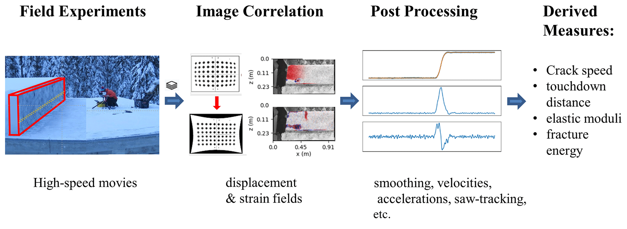
Figure 1Schematic of data processing. After the field experiments were filmed, the frames were analysed using digital image correlation. Displacements obtained with DIC were smoothed to derive velocity and acceleration and thus quantities relevant for crack propagation.
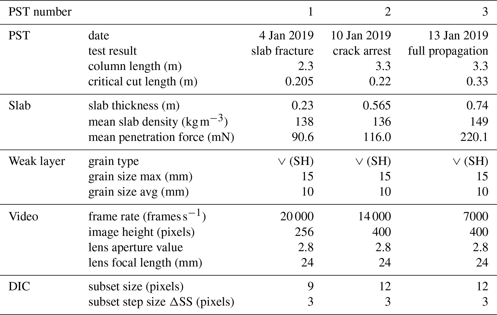
Table 1Overview of experimental parameters and slab and weak layer characteristics from the manual profile and SMP measurements as well as video and DIC analysis parameters for the three flat-field PSTs (slope angle 0∘).
2.2.2 Digital image correlation
For the digital image correlation (DIC) analysis we used DICengine, open-source software provided by Sandia National Laboratories (Turner, 2015). In the images, a region of interest (ROI) was selected encompassing the speckled PST wall. To derive displacement and strain fields of the PST, the ROI was further subdivided into quadratic DIC subsets with a certain side length and step size (Table 1). The position and deformation of each DIC subset was then tracked over time using the first frame of the movie as a reference. In order to find the unique DIC subsets in all subsequent frames, the DIC subsets were allowed to translate, rotate and deform with normal and shear. For an arbitrary DIC subset i, we thus obtained the initial horizontal and vertical position (xi,zi) within the reference image as well as the time (t)-dependent horizontal and vertical displacement ui(t) and wi(t) relative to the initial position, the rotation, normal strain εzz,i(t), and shear strain εxz,i(t).
2.2.3 Post-processing
Since the DIC output is in image space, we first converted it to real space with units of metres. For this, we manually picked a reference length of 2 m in a reference image taken before the experiment to determine the conversion factor. We also changed the origin and orientation of the coordinate system to the upper left corner of the slab with x positive right and z positive downwards.
In the next step, we divided the ROI into three subregions: (i) slab, (ii) weak layer and (iii) substrate. This was performed by drawing an upper and lower boundary of the weak layer manually into the displacement field after fracture. All DIC subsets above the upper boundary were assigned to the slab, all those below the lower boundary to the substrate and all in between to the weak layer.
Since the frame rate of the recorded videos is high compared to crack propagation time, we smoothed the displacements ui(t) and wi(t) using a third-order Savitzky–Golay filter with a window size of 201 frames. To compute velocity and acceleration of the DIC subsets, the first and second derivatives of the smoothed displacement curves were taken (Fig. 1).
2.2.4 Tracking the saw
When sawing into the weak layer, the location of the saw needs to be known to model the resulting slab deformation. We therefore tracked the dot mounted on the tip of the saw using DICengine's tracking functionality (Turner, 2015). Since the dot was not perfectly aligned with the PST side wall, the camera perspective introduced an offset, which was estimated as the mean difference between the automatically tracked cut length rdot and the manually picked cut length rman. We corrected for this offset by (Fig. 2b). Uncertainty in the manual picking was estimated to be 3 pixels (Fig. 2b, transparent red region). For the uncertainty in the automatic tracking we took 3 times the predicted standard deviation of the tracking solution (not visible in Fig. 2b).
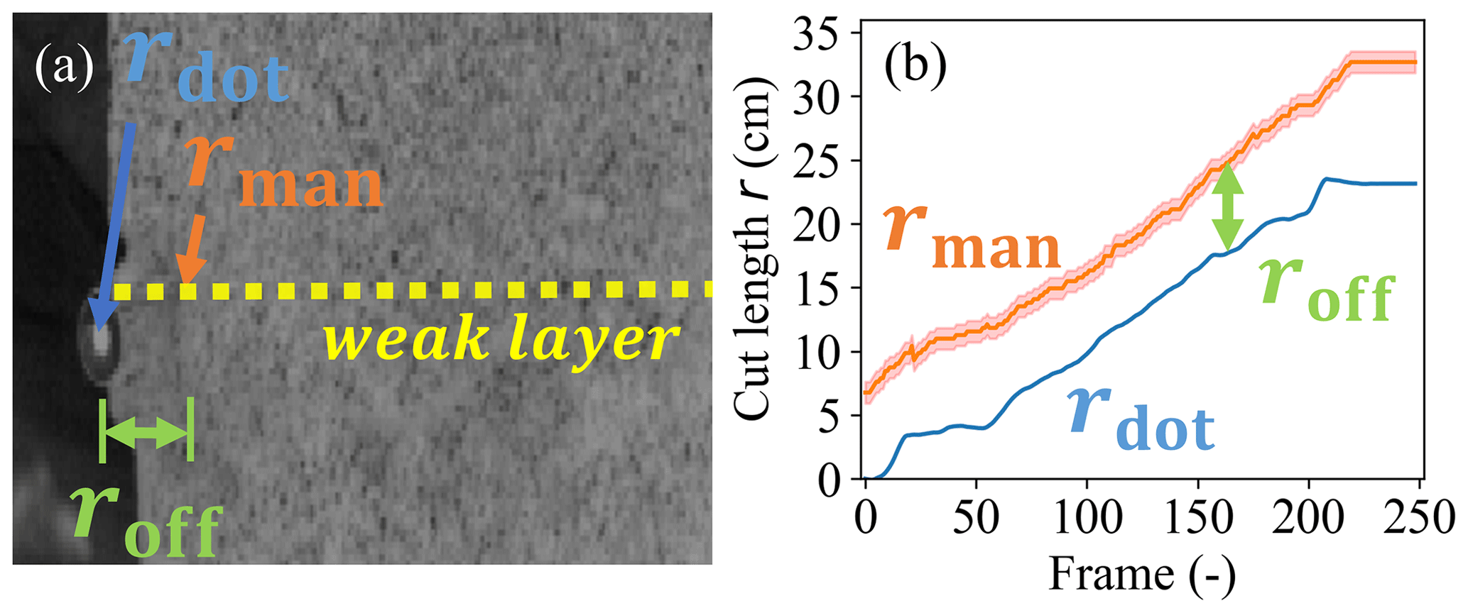
Figure 2(a) Close-up of the saw end of a PST experiment. The saw cut in the weak layer (dashed yellow line) extended to the orange arrow. Due to the camera perspective, the tracked dot on the saw tip (blue arrow) appears at an offset (roff) to the manually estimated saw cut position (rman, orange line in b). (b) The offset between the tracked (blue) and the manually picked cut length (orange) was approximately constant over all frames. Uncertainty is depicted as the transparent red region.
2.3 Mechanical properties
To determine the effective elastic modulus of the slab Esl and the weak layer specific fracture energy wf, a mechanical model is required to fit to the experimental data (e.g. van Herwijnen et al., 2016b). We used two different approaches based on the displacement field and one approach based on SMP measurements.
As a first approach, we followed the methodology described by van Herwijnen et al. (2016b), based on fitting the equation for the mechanical energy provided by Heierli et al. (2008a). We will call this the “VH” method. van Herwijnen et al. (2016b) estimated the effective elastic modulus of the slab and the weak layer specific fracture energy from changes in mechanical energy Vm(r) with cut length r. Using the theorem of Clapeyron, the mechanical energy of the slab is derived from the loss in gravitational potential energy Vp. In our experiments, for a given cut length r, we computed the median z displacement 〈wr(x)〉 for each column in the slab (DIC subsets with the same location x) and summed their contributions to the gravitational potential energy Vp:
where g is the gravitational acceleration. The column mass per unit width was determined as m=ΔSS D ρslab, with ΔSS being the DIC subset step size, D the slab thickness and ρslab the mean slab density (Table 1). Fitting the expression for the mechanical energy (Heierli et al., 2008a; Eqs. 1 and 5) to the data, the slab elastic modulus can be determined (orange line in Fig. 3a). Here, νsl is Poisson's ratio (assumed to be 0.25) and θ is the slope angle. The specific fracture energy of the weak layer is then obtained by numerical differentiation of the mechanical energy at the critical cut length rc. The latter equation holds, independently of the chosen expression for Vm. The only constraint on Vm is that it is zero at the origin (r=0) and that it decreases monotonically with r. We therefore also fitted a power-law function of the form to the data (dashed black line in Fig. 3a) to provide an alternative estimate of the specific fracture energy . To assess the quality of both functions, Vm(r) and f(r), we computed the root mean squared errors, denoted RMSEVH and RMSEFU, respectively.
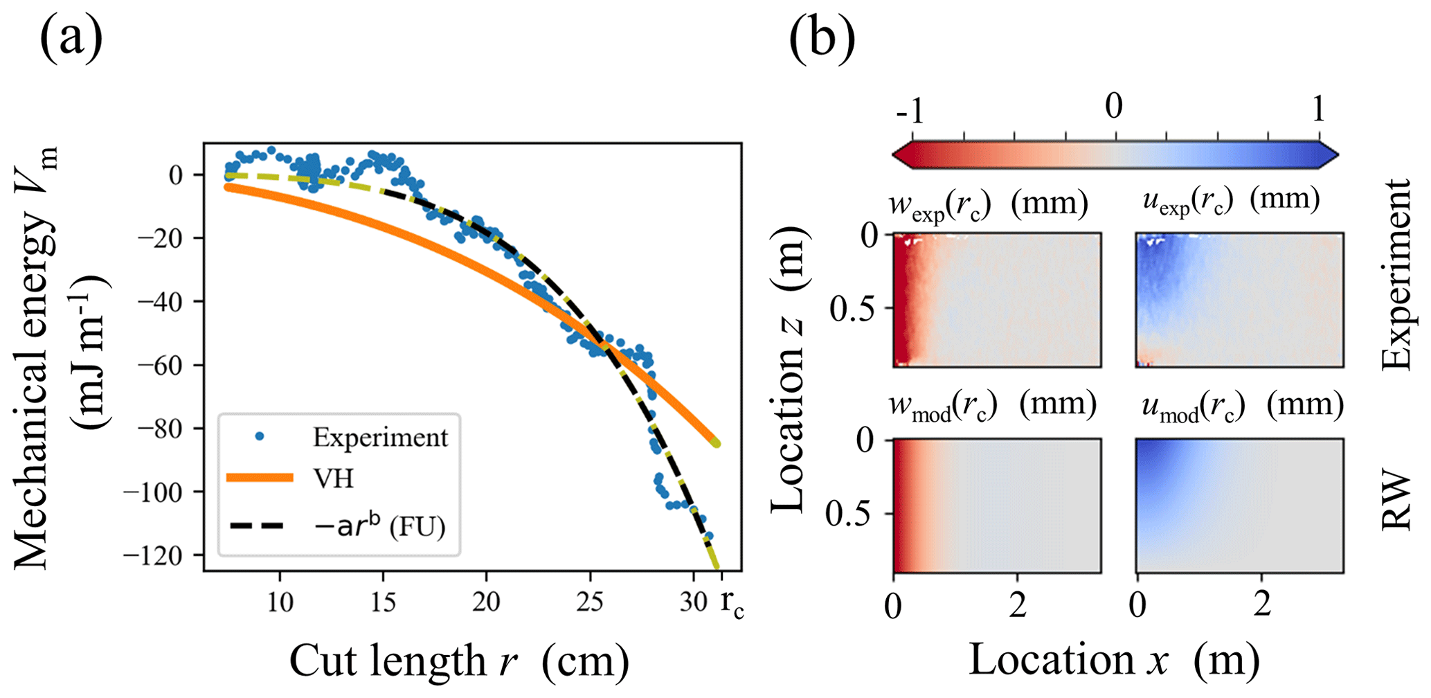
Figure 3(a) Mechanical energy Vm(r) of the slab as a function of cut length r. The orange line is a fit of the theoretical expression of Vm with slab elastic modulus as a free parameter. The dashed black line is a power-law fit to the data. The green sections of the curve are extrapolations of the fits extended to r=rc, where the derivative is taken to estimate the weak layer specific fracture energy and . (b) Vertical (w) and horizontal (u) displacement fields at r=rc in the left and right column, respectively. Measured displacement fields are shown in the top row, while the corresponding modelled displacements using the approach described by Rosendahl and Weissgraeber (2020) are shown in the bottom row.
Second, we used the model suggested by Rosendahl and Weissgraeber (2020), which we will call the “RW” method. Their model considers a Timoshenko beam sitting on a weak layer represented by smeared springs, in contrast to the model of Heierli et al. (2008a), where the weak layer is assumed to be rigid. The RW model predicts horizontal (along the PST column length l, x direction) and vertical (along D, z direction) slab displacements u(x,z) and w(x,z) for different cut lengths r. Required model parameters are the geometrical PST parameters (D, l, θ, column width b and weak layer thickness d); the elastic modulus of the slab and the weak layer (); and Poisson's ratios of the slab (νsl) and the weak layer (νwl), both assumed to be 0.25. To derive and , we computed a residual ε between the measured (uexp,wexp) and modelled (uRW,wRW) displacements (Fig. 3b, top and bottom, respectively):
where the sum is over all DIC subsets SS contained in the slab. Then we used a least-squares optimization routine from SciPy (Virtanen et al., 2020) to find the optimal set of and . The weak layer fracture energy is obtained by
where GI and GII are the contributions from Mode I and Mode II, respectively.
As a third approach, we used SMP measurements. The effective elastic modulus was derived from SMP data as described by Reuter and Schweizer (2018), using the signal interpretation method suggested by Löwe and van Herwijnen (2012). Reuter et al. (2015) suggested a parameterization of the specific fracture energy based on the penetration resistance F(z). Using a moving window (size w=2.5 mm) to integrate F(z), they defined the specific fracture energy as the minimum of the integral within the weak layer:
where A is a fitting parameter. The integration has units of energy (J) and relates to the work required to destroy the snow structure along the integration path. Specific fracture energy, however, has unit energy per area. Therefore, it is necessary to divide by an effective area, the fitting parameter A. While the effective area is unknown, it is likely larger than the cross section of the tip diameter (Johnson, 2003) and depends on snow structure (van Herwijnen, 2013). We therefore followed Reuter et al. (2019) and introduced a fitting parameter A to implicitly account for the unknown effective area. The fitting parameter was derived using a linear regression to PTV-derived specific fracture energies (Fig. 6 in Reuter et al., 2019), resulting in , which relates to a plausible effective cone area of 3.4 cm2 (radius ≈1 cm).
2.4 Crack propagation properties
As characteristics of crack propagation, we computed the temporal evolution of crack speed and touchdown distance for PST experiment no. 3 (PST3), where the crack travelled to the end of the column.
2.4.1 Crack speed
We investigated three methods to derive crack speed. First, we used a method similar to that described by van Herwijnen and Jamieson (2005). As the crack propagates through the weak layer, the weak layer collapses, and displacement curves of DIC subsets in the slab gradually show settlement (Fig. 4a). We used the time delay Δt when the smoothed displacement curves crossed a threshold value of 0.2 mm (the typical standard deviation of w) to determine crack speed (inset in Fig. 4a). The time each DIC subset crossed the threshold value was linked to its x position (blue dots in Fig. 4b). Computing the median for all DIC subsets with the same x location (orange crosses in Fig. 4c), crack speed was then determined as the slope of linear fits in overlapping moving windows (15 cm, step size 3.4 cm, red line in Fig. 4c).
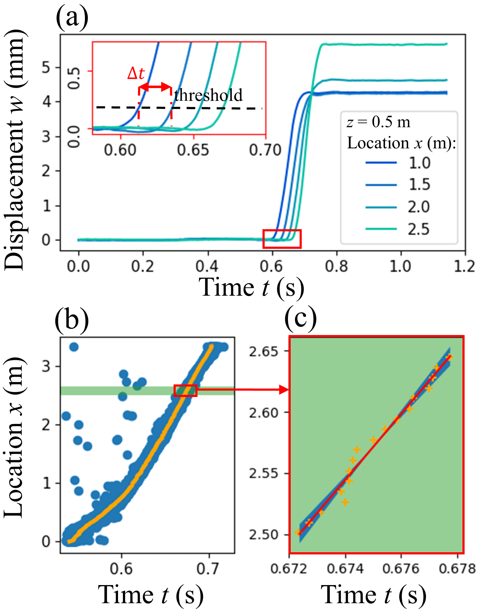
Figure 4(a) Slope-normal displacement with time for four DIC subsets along the PST. Colours indicate the x location of the DIC subsets. The inset shows the displacement threshold (dotted line) used to determine the time difference Δt between the different DIC subsets. (b) Position of DIC subset with time the threshold was passed. Blue dots show individual DIC subsets, while the orange dots show the median of all DIC subsets with the same x location. (c) Position of DIC subset with median time of threshold crossing (orange crosses) for the green area shown in (b). The red line shows the linear fit used to obtain crack speed. The shaded blue areas show the 95 % confidence interval.
Secondly, we used the normal strain from weak layer DIC subsets. Similarly to the displacement-based method, we first smoothed the strain curves εzz,i(t) (Savitzky–Golay filter, window size 31 DIC subsets and order 3) before applying a threshold of −0.01 to the strain in the weak layer. We removed outliers by neglecting time stamps below the 5th percentile and above the 95th percentile. For the remaining time stamps, we calculated the median of all DIC subsets with the same x location before we estimated crack speed cstrain as the slope of linear fits to overlapping moving windows (25 cm, step size 2.5 cm).
Thirdly, we calculated crack speed by cross-correlating the slope-normal acceleration of the DIC subsets. For a given beam section of width Δx=30 cm, we cross-correlated the slope-normal acceleration curves of all DIC subset pairs with the same z location (without repetition) to obtain time lags Δt with pair spacing Δd (Fig. 5). Crack propagation speed was then determined by a linear fit for data pairs of time and pair spacing, Δt vs. Δd. Thus, this approach allowed us to obtain a crack speed estimate ccorr(x) for a specific beam section without having to choose a threshold value.
For all three methods, the uncertainty in the crack speed values was obtained from the 95 % confidence interval of the fit (e.g. blue region in Fig. 4c), and the crack speed over the entire PST experiment was taken as the mean of c(x).
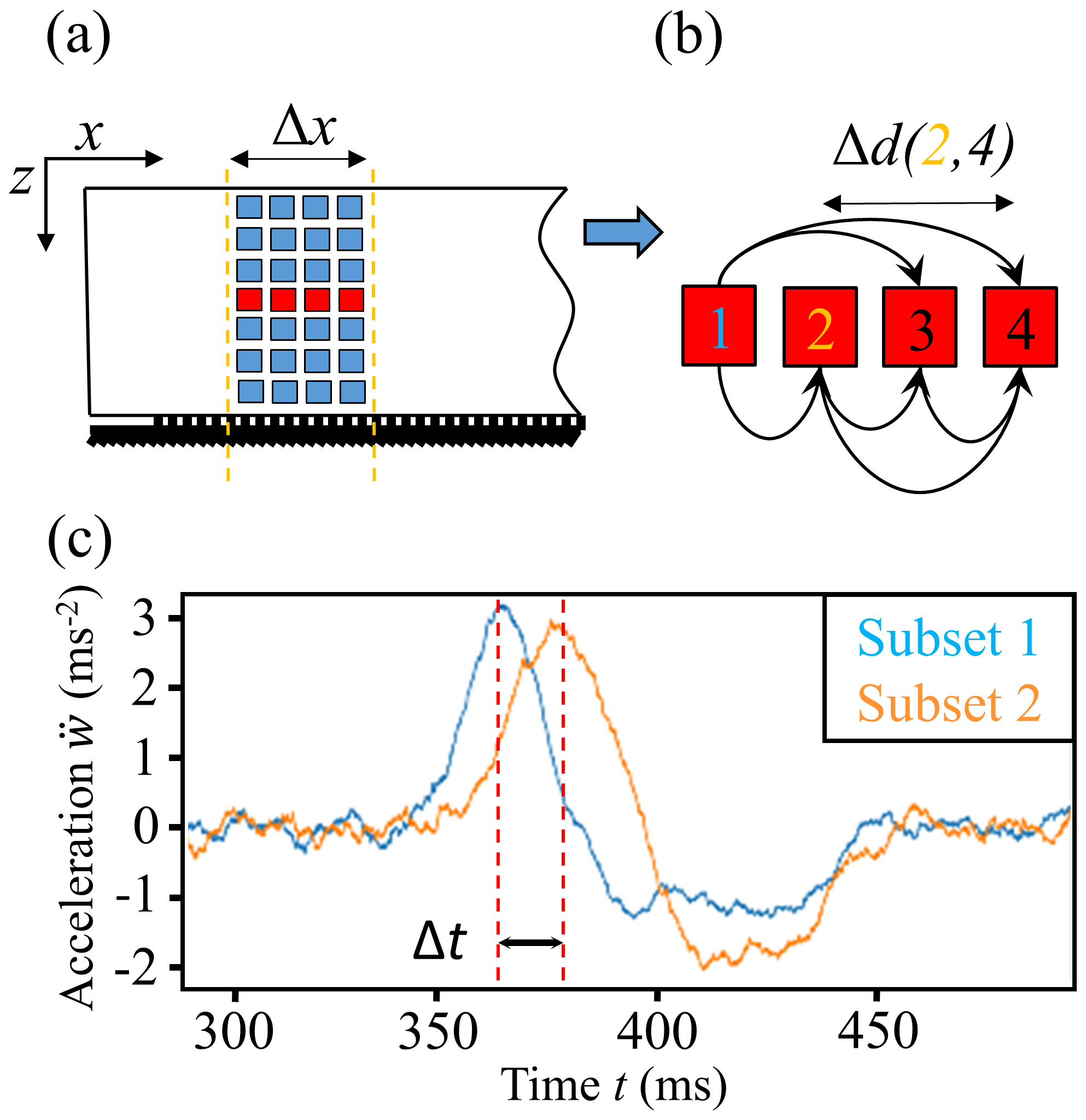
Figure 5(a) For the correlation-based speed estimation we used beam sections containing vertically and horizontally aligned DIC subsets (squares). (b) For a line of DIC subsets (same z location), all possible combinations of DIC subset pairs with a distinct distance Δd are shown (black arrows). (c) By cross-correlating the normal acceleration of a subset pair, we derived the time lag Δt needed to determine crack speed.

Figure 6Raw (solid lines) and smoothed (dashed red lines) vertical velocity of DIC subsets in the slab with x location for different times during crack propagation. At each time step, the touchdown distance λ was estimated as the distance between the two closest subsets that are at rest, i.e. below the threshold value (dashed black line). The touchdown distance at time 0.67 s is shown in red.
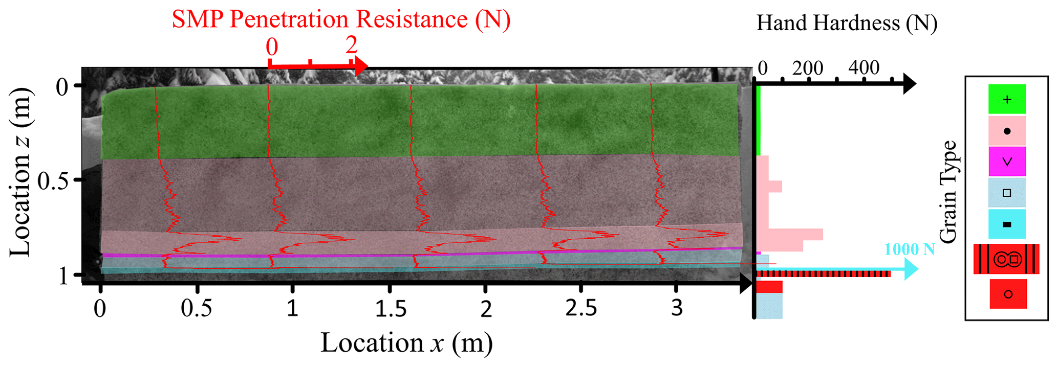
Figure 7SMP-measured penetration resistance (red lines plotted on the PST image) throughout experiment PST3. The colouring of the background corresponds to the layers identified in the manual profile (right side). The manual profile shows the hand hardness index and grain shape indicated by colours (Fierz et al., 2009).
2.4.2 Touchdown distance
As the crack propagates through the PST column, the slab subsides before it comes to rest on the crushed weak layer. As long as a DIC subset in the slab is ahead of the crack tip, it has a slope-normal velocity of zero. The velocity then increases as the crack passes underneath. Finally, as the crack has passed, returns to zero. We therefore defined the length λ as the distance between DIC subsets at rest before and after the collapse. To estimate λ, we averaged normal velocities of all vertically aligned DIC subsets in the slab for each time step (coloured lines in Fig. 6). Then, we performed spatial smoothing along x (Savitzky–Golay, window 61, order 3, dashed red lines in Fig. 6) before applying a threshold of m s−1 to (standard deviation before crack propagation). The touchdown distance λ was then defined as the distance over which subsets exceeded the velocity threshold (red arrow in Fig. 6). The uncertainty in λ was arbitrarily defined as the difference with the value obtained using a 3-times-larger threshold value for .
We analysed three PSTs performed within 10 d in January 2019 at the same site and on the same weak layer consisting of buried surface hoar. We did not note any changes in the weak layer during this period in terms of layer thickness and grain size (Table 1). The thickness of the slab, on the other hand, increased from 23 to 83 cm; the load increased from 318 to 1217 Pa, and mean slab density ranged between 136 and 149 kg m−3. The mean penetration resistance of the slab increased from 90.6 to 220 mN. Overall, the heterogeneity along the three PSTs was negligible and the SMP measurements were in good agreement with manual profiles (e.g. PST3 in Fig. 7).
The critical cut length increased from PST1 to PST3, and crack propagation characteristics were very different. Indeed, PST1 resulted in crack arrest due to a slab fracture (SF), PST2 showed crack arrest (ARR) without slab fracture, and in PST3 the crack propagated to the very end of the column: full propagation (END).
3.1 Displacement and strain
While visual observation of the PSTs in the field allowed us to detect the outcome of PST1 as SF and PST3 as END, we could not discern the result of PST2. We noticed crack propagation did not reach the far end, without seeing obvious indications of where the crack had stopped. It only became clear after consulting the displacement and strain fields that PST2 had resulted in ARR.
For PST3 (END), w(t) increased with time, starting at the sawing end. Total z displacement after weak layer fracture was lowest between positions along the beam. For x>2 m, the total w(t) increased up to 10 mm – about twice as much as for smaller x. This large w(t) is attributed to a secondary crack propagating in the opposite direction, which is particularly clear in the strain field after crack propagation (Fig. 8c3 and Supplement A for the temporal evolution). This secondary crack propagated when the initial crack in the surface hoar weak layer at z=0.8 m reached the far end of the column. The propagation of this secondary crack is also clearly visible in the x displacement (Fig. 8c2). For x<2 m, u(t) returned to zero after crack propagation. For x>2 m, on the other hand, a residual positive x displacement remained after crack propagation (e.g. t=0.8 s). This residual x displacement is grouped into three sections that align very well with the two slab fractures stopping this reverse propagating crack (Video S1 in the Supplement). While in the field we classified PST3 as END, the displacement and strain data clearly show that the crack propagation dynamics were more intricate and a combination of END, SF and ARR. This unexpected result was not recognized in the field.
In PST1 the slab fracture (SF) was visible in the field and also clearly reflected in the measurements, most notably in the strain field (Fig. 9). When the saw reached r=20 cm, a crack within the weak layer started propagating (t=90 ms in Fig. 9b). A tensile crack in the slab then opened at xSF=32 cm (t=120 ms in Fig. 9c) and stopped crack propagation in the weak layer (t=160 ms in Fig. 9d). As the slab fractured, w(t) left of the SF (x<xSF) exhibited downward displacement (positive z) whereas columns very close to xSF showed upward displacement (negative w(t), Fig. 8a1). This suggests that the portion of the slab that became detached rotated with a rotation point close to xSF. The x displacement (mean along z) of all DIC subsets in the detached part of the slab was very similar (blue and green lines in Fig. 8a2).
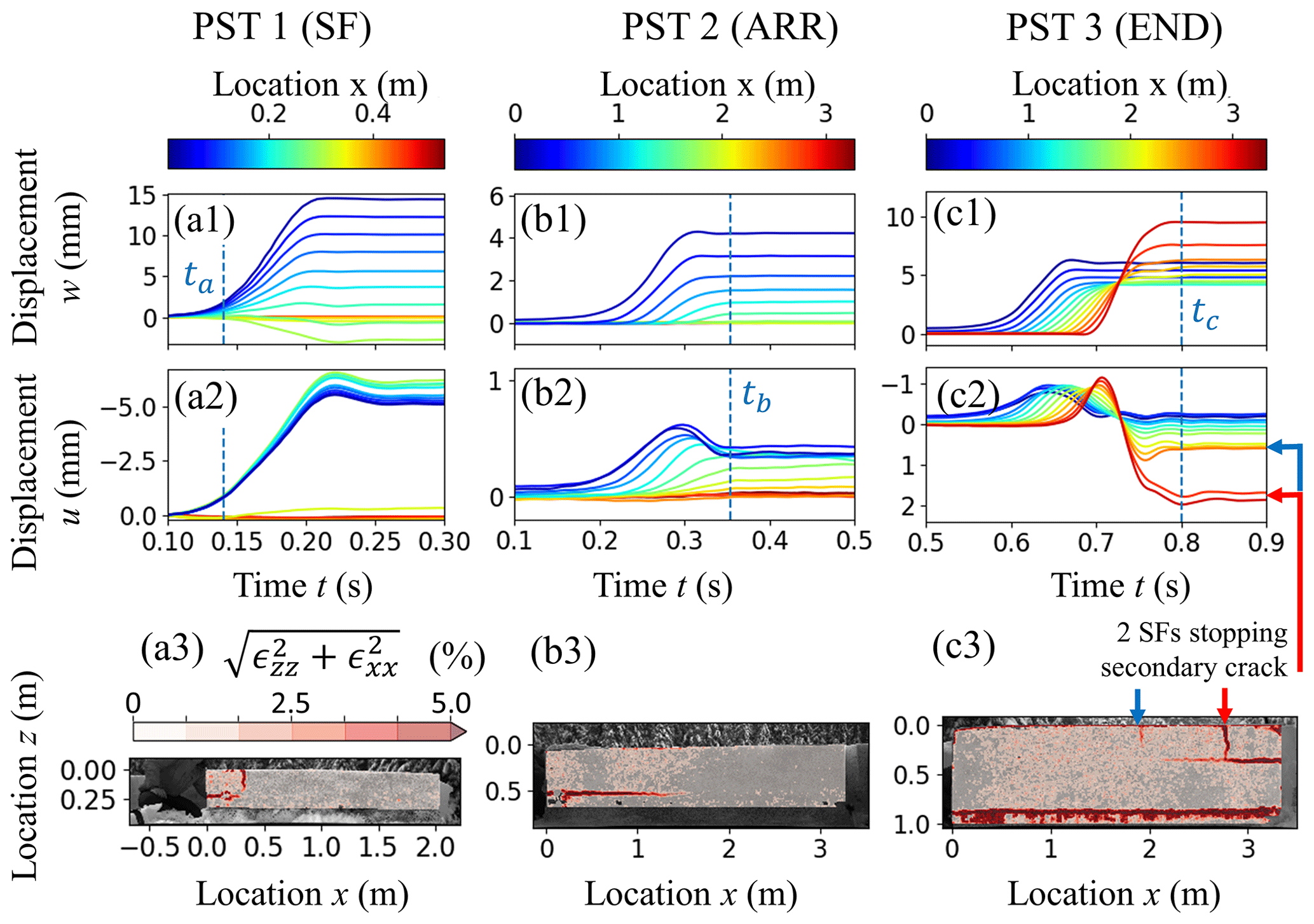
Figure 8Displacement and strain fields for the three different PSTs. (a) Slab fracture, (b) arrest, (c) full propagation. The deformation of the slab with time is shown as displacement curves w (vertical, along z, first row) and u (horizontal, along x, second row) measured at various locations x along the PST beam (colours). The third row shows the strain fields at the respective times ta, tb and tc, indicated with the dashed lines in the upper two rows. Strain concentration around cracks is clearly visible.
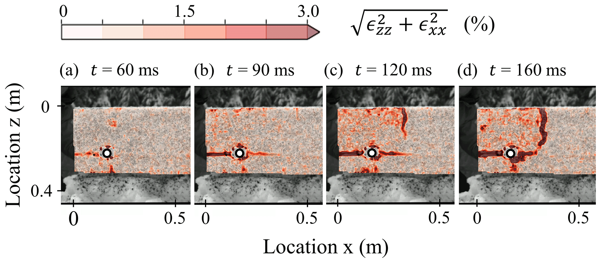
Figure 9Magnitude of normal strains (colours) in the first half metre of PST1 at four different time steps: (a) no weak layer cracking ahead of the snow saw (black circles with white dot), (b) crack propagation ahead of the saw, (c) appearance of a crack in the slab propagating downwards from the snow surface and (d) both cracks are merged.
PST2 resulted in crack arrest (ARR) and the strain at time t=tb at the end of crack propagation was largest in the weak layer, up to a distance of around x=1.6 m (Fig. 8b3). That the crack propagated to this point was also clearly visible in the w(t) of the DIC subsets in the slab. Indeed, the end displacement (t>tb) of the slab decreased continuously with increasing x until no vertical displacement was observed for x>1.6 m (Fig. 8b1). The horizontal displacement u(t), on the other hand, extended beyond the arrested crack tip (), as expected for a bending slab. Interestingly, for x<1.2 m, u(t) decreased after reaching a maximum value before tb, suggesting that the slab experienced some support from the disaggregated weak layer and substrate. This recovered support introduced a bending moment, acting in the opposite direction to the bending moment of the free-hanging beam end.
3.2 Mechanical properties
Depending on the method, the effective elastic modulus of the slab ranged from 1.3 to 5.4 MPa (Table 2). The SMP-based modulus was the average from the five measurements along the PST. Using the RW method, the elastic modulus of the weak layer was also estimated at 0.12 MPa.
To verify the robustness of the derived elastic moduli and , we progressively increased the upper bound of the fit interval rmax from 17 cm to rc (Fig. 10a). Values of rapidly decreased from 22 to 1.8 MPa for rmax=25 cm (orange triangles in Fig. 10a). Subsequently, the decrease was much slower, finally reaching a value of 1.3 MPa at rc. While values of were also larger for shorter fit intervals (blue triangles in Fig. 10a), the decrease was less pronounced than for . Furthermore, and were very consistent for rmax>15 cm (Fig. 10a).
Table 2Effective elastic modulus of the slab and weak layer (Esl and Ewl) as well as the weak layer specific fracture energy wf derived from the VH, RW and BR methods for PST3. For the specific fracture energy wf we additionally used a power-law fit (FU).
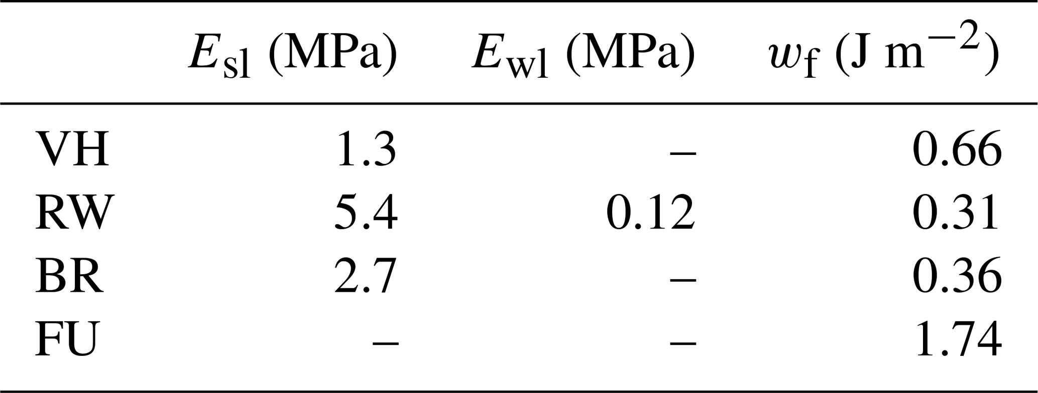
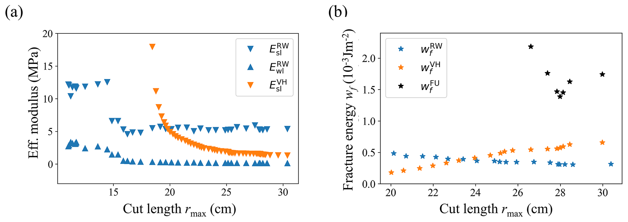
Figure 10(a) Effective elastic moduli estimated with VH ( and RW methods (, using increasing fitting intervals. (b) Weak layer specific fracture energy estimated with RW method (, blue stars), VH method (, orange stars) and a power-law fit (, black stars) using increasing fitting intervals.
Considering the weak layer specific fracture energy wf, the BR and the RW estimates were 0.36 and 0.31 J m−2, respectively, while the VH and FU estimates were higher, 0.66 and 1.7 J m−2, respectively (Table 2). For the VH, RW and FU methods, we quantified the robustness again by checking the trends with increasing cut lengths r (Fig. 10b). Of course, to derive wf both models are evaluated at the critical cut length r=rc, but the computation of wf is based on Esl (and Ewl for the RW method), and Esl is sensitive to changes in the fit interval (r<rmax, VH method) or taking another displacement field (r=rmax, RW method). The spread was largest in , and there were opposite trends in and . Values of for rmax<25 cm were very large (up to 3000 J m−2) and are not shown in Fig. 10b.
3.3 Crack speed and touchdown distance
We used three different methods to estimate the crack speed and its evolution along the PST: the displacement, the strain and the cross-correlation approaches. With the displacement and the strain approaches the crack tip is located using threshold values, while no threshold is required for cross-correlating the acceleration curves. This similarity in methods is also reflected in the comparable values of cdisp and cstrain for PST2 and PST3 (blue and green lines in Fig. 11). Results obtained with the correlation method, on the other hand, were substantially higher and also followed completely different trends throughout the PST experiments (orange lines in Fig. 11).
In PST2 the crack did not reach the far end of the column, and crack speed values were only determined up to the crack arrest point (x=1.6 m, Fig. 11b). Overall, mean cdisp and cstrain values were similar (Table 3) and there was no clear trend throughout the PST (blue and green lines Fig. 11a). In contrast, mean ccorr was much larger, especially near the edges of the PST. For the PST section between 0.7 and 1.3 m, the speed was rather constant with a mean value of .
Table 3Mean crack speeds of PST2 and PST3 estimated with the displacement-based (cdisp), strain-based (cstrain) and correlation-based (ccorr) methods.
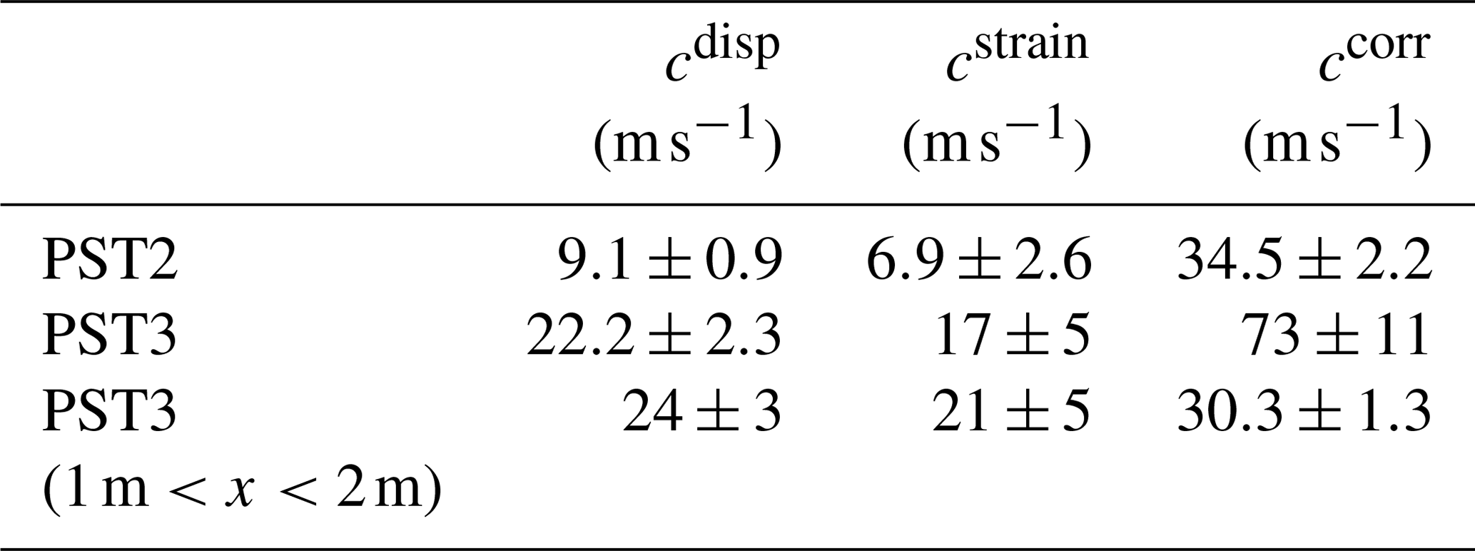
For PST3, cdisp and cstrain were again comparable and exhibited a similar trend across the PST. After an initial increase up to about x=1 m, crack speeds remained rather constant throughout the remainder of the PST (blue and green lines in Fig. 11b). The values of ccorr were again much higher, especially at the beginning and the end of the experiment (Fig. 11a, orange line).

Figure 11Speed estimates along the beam for (a) PST2 and (b) PST3. The speeds are based on the displacement (blue curve), the strain (green line) or the correlation (orange line) methods. The area of the beam that was saw cut (x<rc) is shaded red. The 95 % confidence interval was used to indicate the uncertainty and is depicted as a transparent region behind the corresponding lines.
For PST3, we estimated the length of the touchdown distance λ and its evolution along the PST. As DIC subsets at the beginning of the PST beam came to rest (), the velocity of DIC subsets at x = 2.9 m started exceeding the threshold value, suggesting an initial touchdown distance of 2.9 m. As the crack propagated across the column, λ decreased to around 2.7 m before increasing again towards the far end of the PST (Fig. 12). As λ was only somewhat shorter than the column length, we could only evaluate it within the last 40 cm of crack propagation.
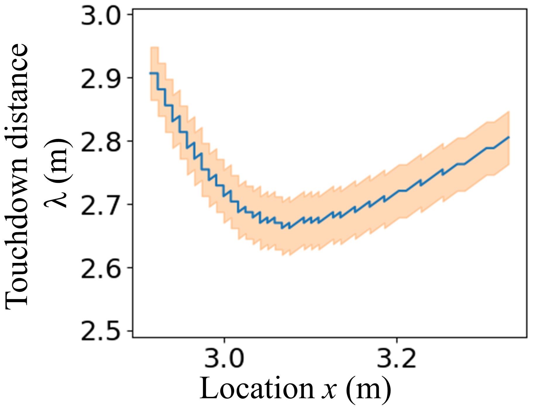
Figure 12Touchdown distance λ in PST3 with crack tip location (blue line). The transparent orange region indicates the uncertainty.
We presented an experimental method to analyse self-sustained crack propagation, i.e. the beginning of dynamic crack propagation, in weak snowpack layers. In this phase, we observed weak layer failure and the associated slab subsidence, in accordance with many previous field studies (van Herwijnen and Jamieson, 2005; van Herwijnen et al., 2010, 2016b; van Herwijnen and Birkeland, 2014). However, in contrast to these previous studies that relied on particle tracking velocimetry (PTV), our use of the DIC method allowed us to observe these processes in much greater detail. For the first time, we were able to measure strain fields in a PST, showing strain concentrations in the area of the weak layer (Fig. 8) as well as in the slab in experiments with slab fractures (Fig. 9). The high frame rate of our video recording combined with the much higher spatial resolution also allowed us to obtain detailed insights into changes in crack speed and touchdown distance during crack propagation.
When observing a PST experiment in the field, it is often very difficult to determine the exact location of crack arrest, distinguish between crack arrest far away from rc and full propagation, or determine whether a slab fracture occurred when the crack arrested. The unusual results obtained for PST3, where full crack propagation occurred followed by a secondary fracture in a different weak layer, were not recognized in the field. With PTV, the method used in previous studies to investigate crack propagation in PSTs, the interpretation of the observed differences in the displacement curves would be ambiguous (Fig. 8c1 to c3). However, the strain field obtained with DIC clearly highlighted the presence of the secondary crack propagating in the opposite direction in a weak snow layer, consisting of precipitation particles closer to the snow surface. This secondary fracture was very likely triggered by the sudden drop of the slab after the crack had propagated through the tested weak layer. The secondary crack was stopped by two slab fractures (Supplement A). These results clearly highlight the advantages of DIC to investigate intricate subtleties occurring in PST experiments and resolve the processes during crack propagation in great detail.
Despite the increased detail obtained with DIC, it was not possible to measure absolute values of strain in the weak layer. The DIC subset size (≈3 cm) was still larger than the vertical extent of the weak layer (≈1.5 cm). Values of strain should thus be considered an average strain over an area with high strain occurring in the weak layer and areas with rigid body motion (portion of the slab, visible in the DIC subset) or even areas without motion (portion of the substrate). Reducing the field of view of the camera would increase spatial measurement resolution; thus by taking close-ups of the weak layer it is theoretically possible to reduce the DIC subset size to less than the extent of the weak layer. However, snow is a porous material consisting of interconnected ice crystals and the thickness of surface hoar layers is often on the same spatial scale as individual crystals. Therefore, the concept of a continuum strain in the weak layer does not exist at this scale, since strain distribution is locally very heterogeneous within the ice matrix. In addition, an appropriate speckling of the measuring surface then becomes difficult, as single crystals would have to be speckled. The strain measurements obtained with DIC therefore show strain localization indicative of crack formation and propagation but cannot be used to accurately quantify the exact deformation behaviour within the weak layer.
4.1 Crack speed and touchdown distance
Thanks to the high frame rates of our recordings, we were able to calculate derivatives of the displacements to obtain speed and acceleration of the DIC subsets. In the past, crack speed and touchdown distance were estimated solely based on displacement data (Bair et al., 2014; van Herwijnen et al., 2010; van Herwijnen and Jamieson, 2005). Here, we exploited speed and acceleration data to derive additional estimates of crack speed and touchdown distance. To estimate these quantities, the position of the crack tip must be known at all times. For opening cracks, the position of the crack tip is the place where the material separates. For closing cracks, as is the case in our experiments, no generally valid definition exists. Therefore, we evaluated similar methods as Bobillier et al. (2021) to estimate crack propagation speed.
We attribute differences in crack speeds obtained in the experiments to the dynamics of crack propagation. With crack extension the load type, strain rate and boundary conditions change, affecting crack growth itself. Slab displacements of DIC subsets, and thus all the variables derived from it, such as speed and acceleration, therefore changed during crack propagation. For instance, in Figs. 8a and 9b the shape of the displacement curves changes along the PST. The various methods used to estimate crack speed were influenced by different aspects of this change in shape. For example, cdisp is sensitive to how rapidly displacement curves initially increase to the threshold value. The correlation method, however, is very sensitive to small changes in the shape of the entire displacement curve, in particular changes in curvature. These shape changes were most pronounced near both ends of the PST, as boundary conditions change, resulting in edge effects (Bair et al., 2014). Hence, in the absence of steady-state crack propagation, the different methods will yield different results.
Looking more closely at the drivers of crack propagation dynamics, two effects can be distinguished. First at the saw end where crack propagation begins, the free-hanging section of the slab steadily grows as long as the slab does not rest on the crushed weak layer. This changes the magnitude and the angle of loading at the location of the crack tip. Second, as the crack approaches the far end of the beam, there are again changes in the magnitude and loading angle at the crack tip as the bending moment in the slab is forced to zero (free boundary). These changes affect the shape of the displacement curves and thus crack speed estimates. In the middle section of the PST, edge effects are less pronounced. Here, possible drivers for crack propagation dynamics are strain rate effects and smaller geometric changes, e.g. changes in touchdown distance. Nevertheless, as long as there is no steady-state crack propagation, slab displacement curves change along the PST column (increasing x location). These changes provide an explanation for the offset observed in the crack speed estimates (Fig. 11). Very long PST experiments would therefore be needed to clarify the existence of steady-state crack propagation (Bobillier et al., 2021; Heierli, 2005). In such experiments, the two prominent dynamical effects (close to column ends and far from column ends) should be more clearly separated. This should allow for measurements of constant crack speed far from the column edges, no matter which method is applied. In our experiments, ccorr was very sensitive to changes in the propagation dynamics, suggesting it is more suited to highlighting edge effects rather than estimating reliable crack speed values. Crack speed estimates of cstrain and cdisp were similar and robust, suggesting that these methods are better suited to estimating crack propagation speeds in PSTs.
While we did not observe steady-state crack propagation within our PSTs, the crack speed values in PST3 can nonetheless be compared with theoretical predictions. Heierli (2005) formulated simple expressions for the crack propagation speed and wavelength of a steady-state collapse wave. With this model, we obtained a wavelength of 2.7 m travelling at a speed of 35 m s−1. The crack speed values around the middle of the PST () ranged from 21 to 30 m s−1 (Table 3), which are somewhat lower than those predicted by the model for steady-state crack propagation. The predicted wavelength and the observed touchdown distance were, however, in good agreement (Fig. 12). To date, only Bair et al. (2014) have reported touchdown distances, and these were much longer than those predicted by theory. They attributed the discrepancy mostly to the model assumption, namely that the slab is in free-fall motion during weak layer collapse. Due to experimental limitations, Bair et al. (2014) could not verify this assumption. In our experiments, however, slab accelerations never exceeded 3 m s−2 (Fig. 5), clearly showing that the slab is not in free fall (Video S1 in the Supplement).
As a practical implication, our results emphasize the need to revisit the predictive power of normal-sized PST experiments. That the measured touchdown distance is longer than the typical PST column length once more shows that normal-sized PSTs cannot reliably predict the propensity for self-sustained crack propagation.
4.2 Elastic modulus and weak layer specific energy
In our study, all estimates of the slab effective modulus were of the same order of magnitude (Table 2). The ratios were approximately . Comparing the moduli derived from the displacement fields, we consider those obtained with the RW method as the most appropriate, as these were more stable with increasing cut lengths (Fig. 10a) and visually the experimental data and the modelled displacements seem to agree very well (Fig. 3). Moreover, with the RW method the elastic modulus of the weak layer can be estimated under the assumptions of isotropy.
For the weak layer specific fracture energy, results were also of the same order of magnitude, although the differences were somewhat larger (). As the formulation of Heierli et al. (2008a) only provided a fair fit to the data (orange line in Fig. 3a), we also fitted a power-law function to the data, resulting into a 2.5-times-larger value of fracture energy. The fracture energy estimates from the SMP data were lower than the VH and FU values. However, the values are considered less reliable as these were obtained using a parameterization based on data obtained with a method very similar to the VH method (Eq. 4). Nevertheless, as the SMP is an efficient instrument to rapidly and objectively measure snowpack parameters in the field, we believe that a comparison with more elaborate methods to estimate specific fracture energy is warranted and may lead to a new parameterization for SMP data.
The RW method provided lower estimates of the specific fracture energy than the VH and FU methods. This might in part be due to limitations of the RW model. Currently, the weak layer in the model can be conceptualized as a set of smeared springs attached to the midsurface of a homogeneous slab. While this reduces the effort of solving the governing equations, the disadvantage is that the Mode II energy release rate GII in flat-field PSTs is always zero as is zero (see Eq. 3 and bottom right in Fig. 3b). One remedy would be to couple the weak layer to the bottom of the slab to determine Mode II specific fracture energies from flat-field experiments as well. Having estimates for both of these independent weak layer material properties would be of interest for better describing mode mixity in weak layer crack propagation.
Overall, the differences in fracture energy estimates clearly highlight that we are not yet able to reliably measure this important material property in snow, beyond order-of-magnitude estimates. Future research should therefore focus on designing tailored field or laboratory experiments to independently measure weak layer fracture energies to validate existing methods.
We recorded PST experiments using a portable high-speed camera. By applying a speckling pattern on the entire side wall of a PST column, we then used digital image correlation (DIC) to derive the displacement and strain of the slab and the strain across the weak layer.
From displacement and strain fields we derived two independent estimates of crack speed (24±3 m s−1 and 21±5 m s−1). In addition, we computed crack speeds by correlating the downward acceleration of the slab in time (30.3±1.3 m s−1). Our results suggest that crack speed can reliably be derived with both threshold-based approaches as these values were in good agreement. Values obtained with the correlation-based technique were, however, susceptible to changes in the shape of the displacement curves and hence to edge effects in the PST. Therefore, values from the correlation-based technique resulted in larger variations in speed along the PST. In general, with our measurement setup and analyses, changes in crack propagation speed at the scale of a PST beam can be investigated.
From the downward velocity field of the slab we estimated the touchdown distance (2.7 m) and its change during crack propagation in a PST. Our results are in good agreement with theoretical predictions from a solitary wave model. However, the model assumption that the slab is in free fall behind the crack tip was refuted based on the observed slab acceleration.
Crack speed and touchdown distance were both affected by edge effects on both free edges of the PST. Our results suggest that much longer PST experiments are required to study the propensity of sustained crack propagation.
While we measured the evolution of strain over the weak layer during crack propagation, it was not possible to determine the true strain within the weak layer due to experimental limitations. The spatial resolution is still too low, since one DIC subset incorporates slab or substrate regions adjacent to the weak layer. In the future, we plan to increase the spatial resolution by filming close-ups around the weak layer, even though a measurement of true strain within the weak layer will probably not be feasible.
Nevertheless, the increased spatial resolution of our DIC setup offered an alternative method for deriving the effective elastic modulus of the slab from the displacement field. Compared to already-established methods, the method based on the model presented by Rosendahl and Weissgraeber (2020) provided a more robust estimate of the effective elastic modulus of the slab and, in addition, of the weak layer.
Finally, we also computed weak layer specific fracture energy. The large variability in our results (0.31–1.74 J m−2) highlights that there is still a need to establish a physically sound and specifically tailored method for measuring weak layer fracture energy.
Overall, this study demonstrates the great potential of the experimental setup and DIC-based analysis methods that in the future should allow for a deeper understanding of the dynamics of crack propagation at the slope scale, which ultimately determines avalanche size.
High-speed recordings and processed data are available on EnviDat: https://doi.org/10.16904/envidat.231 (Bergfeld et al., 2021).
The supplement related to this article is available online at: https://doi.org/10.5194/tc-15-3539-2021-supplement.
JS and AH designed the research and together with BB and GB developed the experimental setup. BB and AH carried out the experimental work. BB processed the high-speed recordings. BR performed the SMP analysis, and JD contributed to all parts of the project. The manuscript was written by BB with input from all authors.
The author Jürg Schweizer is a member of the editorial board of the journal. Bastian Bergfeld, Alec van Herwijnen, Benjamin Reuter, Grégoire Bobillier and Jürg Dual declare that they have no conflict of interest.
Publisher's note: Copernicus Publications remains neutral with regard to jurisdictional claims in published maps and institutional affiliations.
Achille Capelli, Christine Seupel, Colin Lüond, Alexander Hebbe and Simon Caminada assisted with fieldwork. We thank the reviewers, Philipp L. Rosendahl and Edward Bair, for insightful and constructive comments which have helped us significantly improve the manuscript.
This research has been supported by the Schweizerischer Nationalfonds zur Förderung der Wissenschaftlichen Forschung (grant no. 200021_169424).
This paper was edited by Guillaume Chambon and reviewed by Edward Bair and Philipp Rosendahl.
Alfarah, B., López-Almansa, F., and Oller, S.: New methodology for calculating damage variables evolution in Plastic Damage Model for RC structures, Eng. Struct., 132, 70–86, https://doi.org/10.1016/j.engstruct.2016.11.022, 2017.
Bair, E. H., Simenhois, R., van Herwijnen, A., and Birkeland, K.: The influence of edge effects on crack propagation in snow stability tests, The Cryosphere, 8, 1407–1418, https://doi.org/10.5194/tc-8-1407-2014, 2014.
Bergfeld, B., van Herwijnen, A., Bobillier, G., and Schweizer, J.: Measuring slope-scale crack propagation in weak snowpack layers, EGU General Assembly 2020, Online, 4–8 May 2020, EGU2020-8369, https://doi.org/10.5194/egusphere-egu2020-8369, 2020.
Bergfeld, B., van Herwijnen, A., Reuter, B., Bobillier, G., Dual, J., and Schweizer, J.: Dataset for “Dynamic crack propagation in weak snowpack layers: Insights from high-resolution, high-speed photography”, EnviDat, https://doi.org/10.16904/envidat.231, 2021.
Birkeland, K. W., van Herwijnen, A., Reuter, B., and Bergfeld, B.: Temporal changes in the mechanical properties of snow related to crack propagation after loading, Cold Reg. Sci. Technol., 159, 142–152, https://doi.org/10.1016/j.coldregions.2018.11.007, 2019.
Bobillier, G., Bergfeld, B., Dual, J., Gaume, J., van Herwijnen, A., and Schweizer, J.: Micro-mechanical insights into the dynamics of crack propagation in snow fracture experiments, Sci. Rep., 11, 11711, https://doi.org/10.1038/s41598-021-90910-3, 2021.
Bradski, G. and Kaehler, A.: Learning OpenCV, O'Reilly Media Inc., Sebastopol, 2008.
Broberg, K. B.: How fast can a crack go?, Mater. Sci., 32, 80–86, https://doi.org/10.1007/BF02538928, 1996.
Fierz, C., Armstrong, R. L., Durand, Y., Etchevers, P., Greene, E., McClung, D. M., Nishimura, K., Satyawali, P. K., and Sokratov, S. A.: The International Classification for Seasonal Snow on the Ground, HP-VII Technical Documents in Hydrology, IACS Contribution no. 1, UNESCO-IHP, Paris, France, 90 pp., 2009.
Gaume, J., van Herwijnen, A., Gast, T., Teran, J., and Jiang, C.: Investigating the release and flow of snow avalanches at the slope-scale using a unified model based on the material point method, Cold Reg. Sci. Technol., 168, 102847, https://doi.org/10.1016/j.coldregions.2019.102847, 2019.
Gauthier, D. and Jamieson, J. B.: Towards a field test for fracture propagation propensity in weak snowpack layers, J. Glaciol., 52, 164–168, https://doi.org/10.3189/172756506781828962, 2006a.
Gauthier, D. and Jamieson, J. B.: Evaluating a prototype field test for weak layer fracture and failure propagation, Proceedings ISSW 2006, International Snow Science Workshop, Telluride CO, USA, 1–6 October 2006, 107–116, 2006b.
Greene, E., Birkeland, K., Elder, K., McCammon, I., Staples, M., and Sharaf, D.: Snow, Weather, and Avalanches: Observation Guidelines for Avalanche Programs in the United States, 3rd ed., American Avalanche Association, Victor ID, USA, 104 pp., 2016.
Gross, D. and Seelig, T.: Bruchmechanik, 3rd ed., Springer, Berlin, Germany, 317 pp., 2001.
Hamre, D., Simenhois, R., and Birkeland, K.: Fracture speeds of triggered avalanches, Proceedings ISSW 2014, International Snow Science Workshop, Banff, Alberta, Canada, 29 September–3 October 2014, 174–178, 2014.
Heierli, J.: Solitary fracture waves in metastable snow stratifications, J. Geophys. Res., 110, F02008, https://doi.org/10.1029/2004JF000178, 2005.
Heierli, J.: Anticrack model for slab avalanche release, PhD, University of Karlsruhe, Karlsruhe, Germany, 102 pp., 2008.
Heierli, J., Gumbsch, P., and Zaiser, M.: Anticrack nucleation as triggering mechanism for snow slab avalanches, Science, 321, 240–243, https://doi.org/10.1126/science.1153948, 2008a.
Heierli, J., van Herwijnen, A., Gumbsch, P., and Zaiser, M.: Anticracks: A new theory of fracture initiation and fracture propagation in snow, Proceedings ISSW 2008, International Snow Science Workshop, Whistler, Canada, 21–27 September 2008, 9–15, 2008b.
Heierli, J., Gumbsch, P., and Sherman, D.: Anticrack-type fracture in brittle foam under compressive stress, Scripta Mater., 67, 96–99, https://doi.org/10.1016/j.scriptamat.2012.03.032, 2012.
Jamieson, J. B. and Johnston, C. D.: A fracture-arrest model for unconfined dry slab avalanches, Can. Geotech. J., 29, 61–66, https://doi.org/10.1139/t92-007, 1992.
Johnson, J. B.: A statistical micromechanical theory of cone penetration in granular materials, US Army Corps of Engineers, Engineer Research and Development Center, Hanover NH, USA, ERDC/CRREL Technical Report, ERDC/CRREL-TR-03-3, 32, 2003.
Löwe, H. and van Herwijnen, A.: A Poisson shot noise model for micro-penetration of snow, Cold Reg. Sci. Technol., 70, 62–70, https://doi.org/10.1016/j.coldregions.2011.09.001, 2012.
Marshall, H.-P. and Johnson, J. B.: Accurate inversion of high-resolution snow penetrometer signals for microstructural and micromechanical properties, J. Geophys. Res., 114, F04016, https://doi.org/10.1029/2009jf001269, 2009.
McClung, D. M.: Approximate estimates of fracture speeds for dry slab avalanches, Geophys. Res. Lett., 32, L08406, https://doi.org/10.1029/2005GL022391, 2005.
McClung, D. M. and Schaerer, P.: The Avalanche Handbook, 3rd ed., The Mountaineers Books, Seattle WA, USA, 342 pp., 2006.
Pudasaini, S. P. and Hutter, K.: Avalanche dynamics: Dynamics of rapid flows of dense granular avalanches, Springer, Berlin, Heidelberg, Germany, 602 pp., 2007.
Reuter, B. and Schweizer, J.: Describing snow instability by failure initiation, crack propagation, and slab tensile support, Geophys. Res. Lett., 45, 7019–7027, https://doi.org/10.1029/2018GL078069, 2018.
Reuter, B., Proksch, M., Löwe, H., van Herwijnen, A., and Schweizer, J.: On how to measure snow mechanical properties relevant to slab avalanche release, Proceedings ISSW 2013, International Snow Science Workshop, Grenoble, France, 7–11 October 2013, 7–11, 2013.
Reuter, B., Schweizer, J., and van Herwijnen, A.: A process-based approach to estimate point snow instability, The Cryosphere, 9, 837–847, https://doi.org/10.5194/tc-9-837-2015, 2015.
Reuter, B., Proksch, M., Löwe, H., van Herwijnen, A., and Schweizer, J.: Comparing measurements of snow mechanical properties relevant for slab avalanche release, J. Glaciol., 65, 55–67, https://doi.org/10.1017/jog.2018.93, 2019.
Rosendahl, P. L. and Weißgraeber, P.: Modeling snow slab avalanches caused by weak-layer failure – Part 1: Slabs on compliant and collapsible weak layers, The Cryosphere, 14, 115–130, https://doi.org/10.5194/tc-14-115-2020, 2020.
Schneebeli, M. and Johnson, J. B.: A constant-speed penetrometer for high-resolution snow stratigraphy, Ann. Glaciol., 26, 107–111, https://doi.org/10.3189/1998AoG26-1-107-111, 1998.
Schweizer, J., Jamieson, J. B., and Schneebeli, M.: Snow avalanche formation, Rev. Geophys., 41, 1016, https://doi.org/10.1029/2002RG000123, 2003.
Schweizer, J., van Herwijnen, A., and Reuter, B.: Measurements of weak layer fracture energy, Cold Reg. Sci. Technol., 69, 139–144, https://doi.org/10.1016/j.coldregions.2011.06.004, 2011.
Schweizer, J., Bartelt, P., and van Herwijnen, A.: Snow avalanches, in: Snow and Ice-Related Hazards, Risks, and Disasters, 2nd ed., edited by: Haeberli, W. and Whiteman, C., Elsevier, Amsterdam, the Netherlands, 377–416, 2021.
Sigrist, C. and Schweizer, J.: Critical energy release rates of weak snowpack layers determined in field experiments, Geophys. Res. Lett., 34, L03502, https://doi.org/10.1029/2006GL028576, 2007.
Sigrist, C., Schweizer, J., Schindler, H. J., and Dual, J.: On size and shape effects in snow fracture toughness measurements, Cold Reg. Sci. Technol., 43, 24–35, https://doi.org/10.1016/j.coldregions.2005.05.001, 2005.
Sigrist, C., Schweizer, J., Schindler, H. J., and Dual, J.: Measurement of fracture mechanical properties of snow and application to dry snow slab avalanche release, Geophysical Research Abstracts, 8, 08760, 2006.
Trottet, B., Simenhois, R., Bobillier, G., van Herwijnen, A., Jiang, C., and Gaume, J.: From sub-Rayleigh to intersonic crack propagation in snow slab avalanche release, EGU General Assembly 2021, online, 19–30 Apr 2021, EGU21-8253, https://doi.org/10.5194/egusphere-egu21-8253, 2021.
Turner, D. Z.: Digital Image Correlation Engine (DICe) Reference Manual, National Technology & Engineering Solutions of Sandia, Albuquerque, New Mexico, USA, SAND2015-10606 O, 2015.
van Herwijnen, A.: Experimental analysis of snow micropenetrometer (SMP) cone penetration in homogeneous snow layers, Can. Geotech. J., 50, 1044–1054, https://doi.org/10.1139/cgj-2012-0336, 2013.
van Herwijnen, A. and Birkeland, K. W.: Measurements of snow slab displacement in Extended Column Tests and comparison with Propagation Saw Tests, Cold Reg. Sci. Technol., 97, 97–103, https://doi.org/10.1016/j.coldregions.2013.07.002, 2014.
van Herwijnen, A. and Heierli, J.: In-situ measurement of the mechanical energy associated with crack growth in weak snowpack layers and determination of the fracture energy, Geophysical Research Abstracts, 12, 11743, 2010.
van Herwijnen, A. and Jamieson, B.: High-speed photography of fractures in weak snowpack layers, Cold Reg. Sci. Technol., 43, 71–82, https://doi.org/10.1016/j.coldregions.2005.05.005, 2005.
van Herwijnen, A., Schweizer, J., and Heierli, J.: Measurement of the deformation field associated with fracture propagation in weak snowpack layers, J. Geophys. Res., 115, F03042, https://doi.org/10.1029/2009JF001515, 2010.
van Herwijnen, A., Bair, E. H., Birkeland, K. W., Reuter, B., Simenhois, R., Jamieson, B., and Schweizer, J.: Measuring the mechanical properties of snow relevant for dry-snow slab avalanche release using particle tracking velocimetry, Proceedings ISSW 2016, International Snow Science Workshop, Breckenridge CO, USA, 3–7 October 2016, 397–404, 2016a.
van Herwijnen, A., Gaume, J., Bair, E. H., Reuter, B., Birkeland, K. W., and Schweizer, J.: Estimating the effective elastic modulus and specific fracture energy of snowpack layers from field experiments, J. Glaciol., 62, 997–1007, https://doi.org/10.1017/jog.2016.90, 2016b.
Virtanen, P., Gommers, R., Oliphant, T. E., Haberland, M., Reddy, T., Cournapeau, D., Burovski, E., Peterson, P., Weckesser, W., Bright, J., van der Walt, S. J., Brett, M., Wilson, J., Millman, K. J., Mayorov, N., Nelson, A. R. J., Jones, E., Kern, R., Larson, E., Carey, C. J., Polat, İ., Feng, Y., Moore, E. W., VanderPlas, J., Laxalde, D., Perktold, J., Cimrman, R., Henriksen, I., Quintero, E. A., Harris, C. R., Archibald, A. M., Ribeiro, A. H., Pedregosa, F., van Mulbregt, P., Vijaykumar, A., Bardelli, A. P., Rothberg, A., Hilboll, A., Kloeckner, A., Scopatz, A., Lee, A., Rokem, A., Woods, C. N., Fulton, C., Masson, C., Häggström, C., Fitzgerald, C., Nicholson, D. A., Hagen, D. R., Pasechnik, D. V., Olivetti, E., Martin, E., Wieser, E., Silva, F., Lenders, F., Wilhelm, F., Young, G., Price, G. A., Ingold, G.-L., Allen, G. E., Lee, G. R., Audren, H., Probst, I., Dietrich, J. P., Silterra, J., Webber, J. T., Slavič, J., Nothman, J., Buchner, J., Kulick, J., Schönberger, J. L., de Miranda Cardoso, J. V., Reimer, J., Harrington, J., Rodríguez, J. L. C., Nunez-Iglesias, J., Kuczynski, J., Tritz, K., Thoma, M., Newville, M., Kümmerer, M., Bolingbroke, M., Tartre, M., Pak, M., Smith, N. J., Nowaczyk, N., Shebanov, N., Pavlyk, O., Brodtkorb, P. A., Lee, P., McGibbon, R. T., Feldbauer, R., Lewis, S., Tygier, S., Sievert, S., Vigna, S., Peterson, S., More, S., Pudlik, T., Oshima, T., Pingel, T. J., Robitaille, T. P., Spura, T., Jones, T. R., Cera, T., Leslie, T., Zito, T., Krauss, T., Upadhyay, U., Halchenko, Y. O., Vázquez-Baeza, Y., and SciPy 1.0 Contributors: SciPy 1.0: fundamental algorithms for scientific computing in Python, Nat. Methods, 17, 261–272, https://doi.org/10.1038/s41592-019-0686-2, 2020.
Walters, D. J. and Adams, E. E.: Quantifying anisotropy from experimental testing of radiation recrystallized snow layers, Cold Reg. Sci. Technol., 97, 72–80, https://doi.org/10.1016/j.coldregions.2013.09.014, 2014.
dynamic crack propagation phasein which a whole slope becomes detached. The present work contains the first field methodology which provides the temporal and spatial resolution necessary to study this phase. We demonstrate the versatile capabilities and accuracy of our method by revealing intricate dynamics and present how to determine relevant characteristics of crack propagation such as crack speed.
dynamic crack...