the Creative Commons Attribution 4.0 License.
the Creative Commons Attribution 4.0 License.
 | 29 Jul 2021
Two-dimensional impurity imaging in deep Antarctic ice cores: snapshots of three climatic periods and implications for high-resolution signal interpretation
Marco Roman
Martin Šala
Barbara Delmonte
Barbara Stenni
Carlo Barbante
Due to its micrometer-scale resolution and inherently micro-destructive nature, laser ablation inductively coupled plasma mass spectrometry (LA-ICP-MS) is particularly suited to exploring the thin and closely spaced layers in the oldest sections of polar ice cores. Recent adaptions to the LA-ICP-MS instrumentation mean we have faster washout times allowing state-of-the-art 2-D imaging of an ice core. This new method has great potential especially when applied to the localization of impurities on the ice sample, something that is crucial, to avoiding misinterpretation of the ultra-fine-resolution signals. Here we present the first results of the application of LA-ICP-MS elemental imaging to the analysis of selected glacial and interglacial samples from the Talos Dome and EPICA Dome C ice cores from central Antarctica. The localization of impurities from both marine and terrestrial sources is discussed, with special emphasis on observing a connection with the network of grain boundaries and differences between different climatic periods. Scale-dependent image analysis shows that the spatial significance of a single line profile along the main core axis increases systematically as the imprint of the grain boundaries weakens. It is demonstrated how instrumental settings can be adapted to suit the purpose of the analysis, i.e., by either employing LA-ICP-MS to study the interplay between impurities and the ice microstructure or to investigate the extremely thin climate proxy signals in deep polar ice.
- Article
(15231 KB) - Full-text XML
-
Supplement
(963 KB) - BibTeX
- EndNote


Antarctic ice cores are a cornerstone of modern paleoclimatic research, archiving a unique variety of proxies such as greenhouse gases and aerosol-related atmospheric impurities over timescales from decades to hundreds of millennia (e.g., Petit et al., 1999; Kawamura et al., 2003; Ahn et al., 2004; EPICA Community Members, 2004). Investigation of the oldest, deepest and thinnest ice core layers has become of special interest in state-of-the-art polar ice core research since the search has begun for a 1.5-million-year-old record that could be recovered from Antarctica (Brook et al., 2006; Fischer et al., 2013). It is expected that 10 000 years worth of climatic record could be recovered from within each meter of the deepest ice core sections (Lilien et al., 2021). The goal to obtain this record at the finest detail drives the demand for new analytical methods that surpass the depth resolution capabilities of established methods based on meltwater analysis, such as continuous flow analysis (CFA) (e.g., Röthlisberger et al., 2000; McConnell et al., 2002; Osterberg et al., 2006; Kaufmann et al., 2008). Within this framework, laser ablation inductively coupled plasma mass spectrometry (LA-ICP-MS) has recently been re-established as a high-resolution trace element technique for the characterization of ice cores (Müller et al., 2011; Sneed et al., 2015). Comparison of the LA-ICP-MS signals with CFA has revealed that the low-frequency variability seen in LA-ICP-MS signals is consistent with the full-resolution impurity records obtained by CFA (Della Lunga et al., 2017; Spaulding et al., 2017). Initial investigations were also performed regarding the relationship between LA-ICP-MS signals and the abundantly observed ice crystal features such as grain boundaries and triple junctions (Della Lunga et al., 2014, 2017; Kerch, 2016; Beers et al., 2020). Advances made by employing dedicated ablation cells with fast washout as well as optimizing the lasing and ICP-MS settings have introduced a new state of the art in imaging techniques with LA-ICP-MS (Wang et al., 2013; van Elteren et al., 2019). The term “washout time” refers to the time needed to transfer the ablated sample aerosol plume to the ICP-MS. It is principally determined by the extraction efficiency from the ablation cell and any subsequent dispersion in the transfer line. With washout times in the tens of milliseconds range, the recording of baseline-separated single pulses at high repetition rates becomes possible (Van Malderen et al., 2015). Recently, this new imaging approach was transferred to ice core analysis with LA-ICP-MS, offering the opportunity to study the distribution of impurities in ice cores in 2-D. First results clearly demonstrated a close connection between grain boundaries and high-resolution LA-ICP-MS signals, which became particularly evident for example for sodium (Bohleber et al., 2020).
As a result of these developments, LA-ICP-MS promises to be a tool for locating impurities in the ice matrix, supplementing methods such as scanning electron microscopy equipped with energy-dispersive X-ray spectroscopy (SEM-EDS) (Barnes et al., 2003; Barnes and Wolff, 2004; Iliescu and Baker, 2008) and micro-Raman spectroscopy (Sakurai et al., 2011; Eichler et al., 2017). Understanding the micro-scale impurity localization is not only important for the deformational (Dahl-Jensen et al., 1997) and dielectric properties (Stillman et al., 2013) of glacier ice on a macroscopic scale. It also becomes especially important when assessing the stratigraphic integrity of high-resolution impurity records in deep and comparatively warm ice, which is typically characterized by large ice grains (Faria et al., 2014a). This is particularly important for soluble species, where the advection of impurity anomalies, through diffusion along the ice vein network, has been discussed as a possible cause of post-depositional alterations in ice core paleoclimate records (Rempel et al., 2001; Ng, 2021).
Impurity localization at the grain boundaries also has direct consequences on the interpretation of 1-D LA-ICP-MS profiles, i.e., single lines measured along the main core axis. Such line profiles have been used to obtain a high-resolution time series of paleoclimate signals, after further smoothing (e.g., Mayewski et al., 2014; Haines et al., 2016; Della Lunga et al., 2017). It has been suggested that, in the presence of signal imprints related to the ice crystal matrix, it may be beneficial to average the signal between two or more parallel tracks (Della Lunga et al., 2017). A standardization technique has not yet been developed, however. It quickly becomes evident that the signal reproducibility of parallel line tracks will depend on local variations in grain sizes and in the imprint of the grain boundaries. In this context, 2-D imaging can provide a more refined approach in assessing the origin of the LA-ICP-MS signal and the spatial significance of single line profiles.
To trial the recently developed LA-ICP-MS imaging techniques (Bohleber et al., 2020) for Antarctic ice cores, samples of various depth sections were selected that were representative of distinct climatic periods. The samples were analyzed, aiming to include a broad spectrum of ice properties, such as age and mean grain size. These snapshots of the 2-D impurity distribution taken by LA-ICP-MS elemental imaging provide important details on the location of impurities in relation to the grain boundary network. The imprint of the grain boundaries may vary between different impurity species and climatic periods. Consequently, the spatial significance of a single line profile along the main core axis has to be carefully assessed. These 2-D images provide new and improved information for this purpose. It has also been shown how measurement settings can be adapted, so LA-ICP-MS line profiles can be used when investigating climate proxy signals in highly thinned deep polar ice.
Table 1Samples from Antarctic ice cores analyzed by LA-ICP-MS impurity imaging.
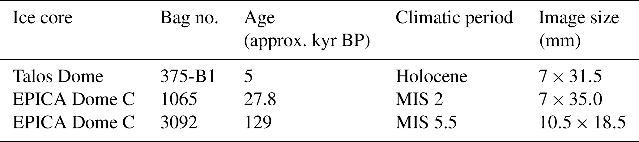
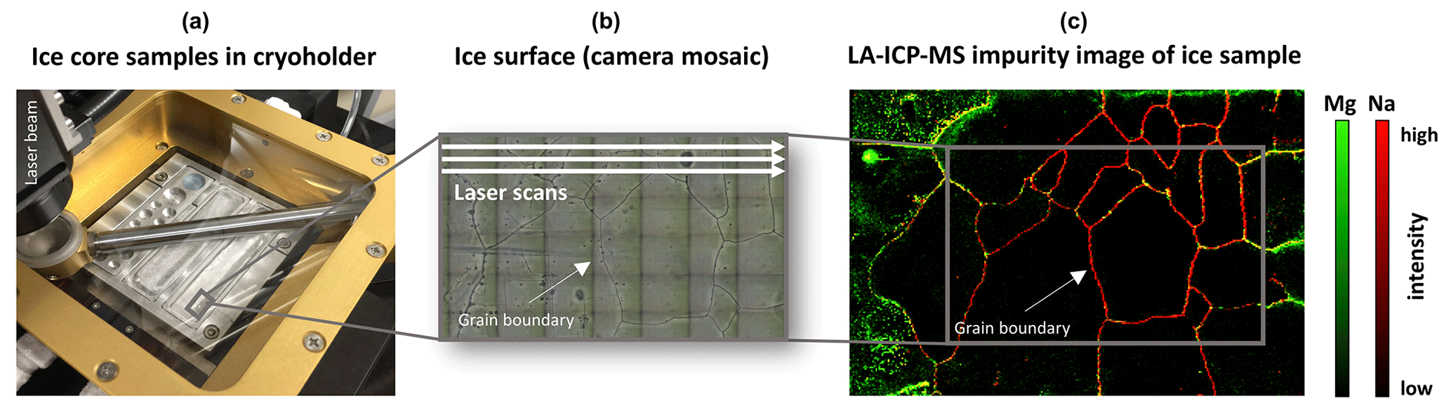
Figure 1Generating 2-D impurity images of ice cores by LA-ICP-MS. Strips of ice (approx. 9×2, 1.5 cm thickness) are kept frozen in a custom-designed cryogenic holder (a). A mosaic of optical images allows localizing ice surface features such as grain boundaries (b). Data from an array of non-overlapping laser scan lines are stacked without interpolation to generate an elemental map of impurities distribution (c).
The LA-ICP-MS setup employed at the University of Venice comprises of an Analyte Excite ArF excimer 193 nm laser (Teledyne CETAC Photon Machines) and an iCAP-RQ quadrupole ICP-MS (Thermo Scientific). The laser ablation system includes a HelEx II two-volume ablation cell mounted on a high-precision xy stage equipped with a custom-built cryogenic sample holder to keep the ice core samples below their freezing point. The circulation of a glycol–water mixture cooled to C keeps the surface temperature of the ice samples consistently at C. Established procedures for ice sample preparation and surface decontamination for the LA-ICP-MS of ice core analysis were followed (Della Lunga et al., 2014, 2017). A band saw was used in a cold room (C) to cut ice samples into 9×2 cm strips. Ice thickness was then reduced to 1.5 cm by manual scraping using a custom-built PTFE vice with a ceramic ZrO2 blade (American Cutting Edge, USA).
Helium was used as the carrier gas for aerosol transport from the sample surface to the ICP-MS. As an important addition, ARIS, a rapid aerosol transfer line, was used, resulting in a washout time of ∼34 ms. A repetition rate of 294 Hz and a dosage of 10 was used here. In contrast to single pulse analysis, a dosage greater than 1 implies that each pixel is generated by multiple partially overlapping laser shots, which leads to an improved signal-to-noise ratio and better image quality (Šala et al., 2021). The fast washout combined with a high repetition rate allows scanning of the surface at around 1 mm s−1, which is roughly 10 times faster than previous studies on ice cores (Della Lunga et al., 2017; Spaulding et al., 2017). As a result, artifact-free elemental maps can be generated at high spatial resolution in a limited run time and/or over comparatively large areas (van Elteren et al., 2019).
Firstly, at least one full pre-ablation run was conducted to further decontaminate the sample, using a square spot size of 150×150 µm as well as bidirectional scanning. Next, the maps were obtained as a pattern of lines with a 35×35 µm square spot size, at a laser fluence of 3.5 J cm−2, without overlap perpendicular to the scan direction, and without any post-acquisition spatial interpolation. Lateral resolution is 35 µm both along and perpendicular to the scan direction. Due to the precise synchronization of data acquisition required to avoid image artifacts, the number of analytes/isotopes was restricted. Four elements were routinely recorded per image: 23Na, 25Mg, 55Mn and 88Sr with respective ICP-MS dwell times of 4, 4.6, 10 and 10 ms. (Bohleber et al., 2020). The total sweep time was 34 ms, specifically set to match the washout time, resulting in a total duty cycle of 84 %. Considered in the following are Na, Mg and Sr, due to their significance as paleoclimate proxies in polar ice cores (Legrand and Mayewski, 1997): Na being related mostly to sea salt, Mg with both marine and terrestrial sources and Sr as a chemically similar substitute for Ca, which is mostly related to terrestrial sources. Ca is analytically challenging with ICP-MS due to significant spectral interferences. Scan lines on a NIST glasses SRM 612 and 614 were measured before and after the acquisition of each map. Background and drift correction as well as image construction were performed using the software HDIP (Teledyne Photon Machines, Bozeman, MT, USA).
Using the integrated camera co-aligned with the laser, it is possible to obtain a mosaic of optical images of the ice sample surface. Here, it becomes possible to see entrapped air bubbles (dark circles) and to distinguish individual ice crystals and their boundaries (dark lines). Comparing such optical images with the LA-ICP-MS elemental maps allows a clear assessment of the localization of impurities within the ice crystal matrix (Fig. 1). Further details of the ice core impurity imaging method have already been described elsewhere (Bohleber et al., 2020).
Our sample selection, targeted ice at various depth sections and climatic periods in Antarctic ice cores, including glacial as well as interglacial periods. At the same time, the deepest sections were avoided since they featured very large grain size that call for mapping of large areas (see Discussion). For the purpose of this study, the analysis focused on three exemplary datasets with the highest image quality (Table 1). The Talos Dome Holocene ice sample (referred to in the following as TD Holocene) is from a depth section featuring an average grain size of 1–2 mm (Montagnat et al., 2012). Likewise, the EPICA Dome C core (EDC) at a depth of 585.2 m corresponds to Marine Isotope Stage 2 (EDC MIS 2) and has an average grain radius of around 1.5 mm. Notably, this sample is also from a section characterized by a very high dust content (average around 500 µg kg−1). In contrast, the sample from MIS 5.5 (EDC MIS 5.5) is from 1700.5 m depth and is characterized by low dust levels but a local maximum in grain radius at around 3.5 mm (EPICA Community Members, 2004).
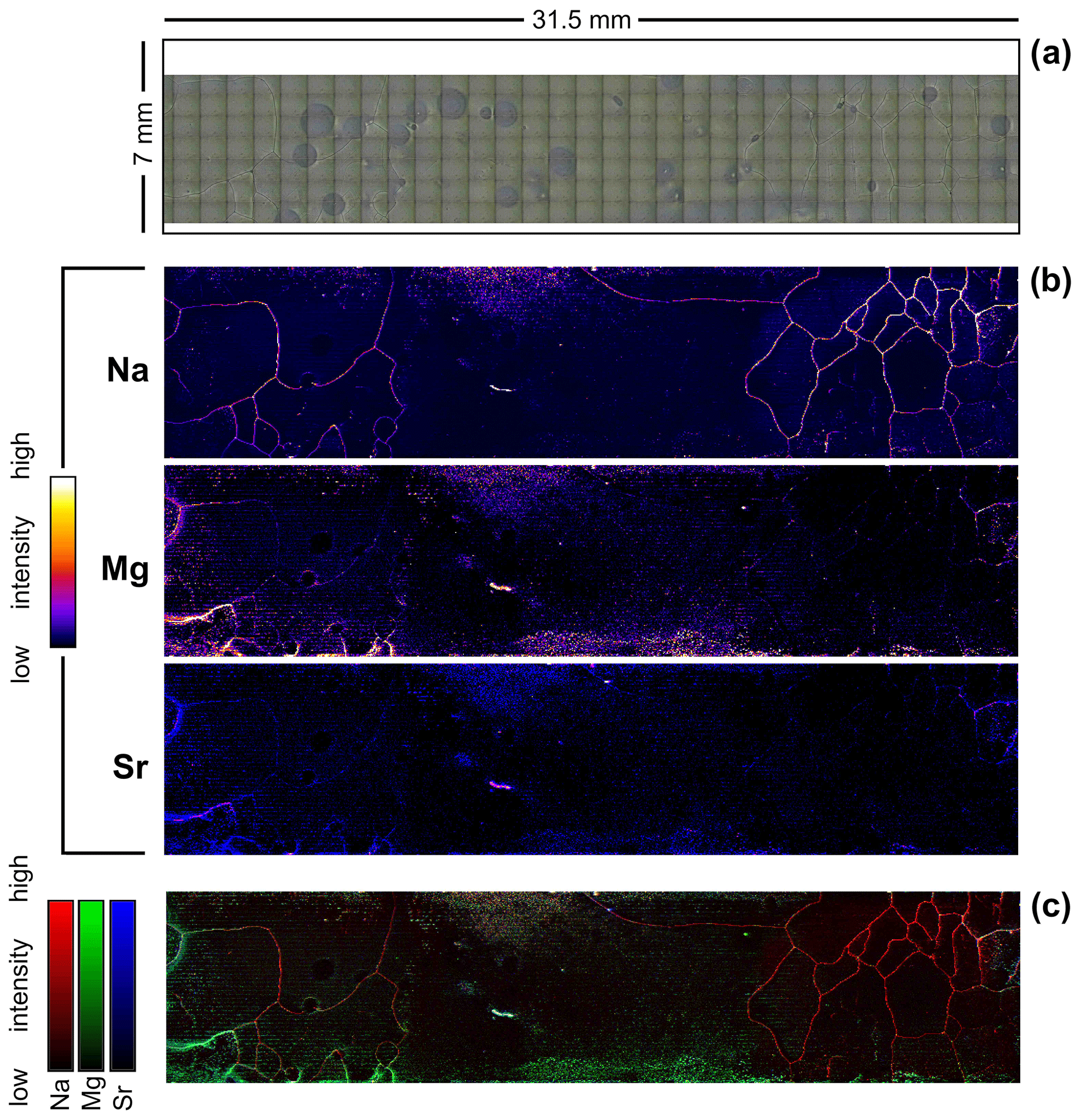
Figure 2Talos Dome 375-B1 Holocene sample. Panel (a) shows an optical image; panel (b) elemental maps of Na, Mg and Sr, respectively, for the same area; (c) composite RGB map of the three elements. The main core axis runs from left (top) to right.
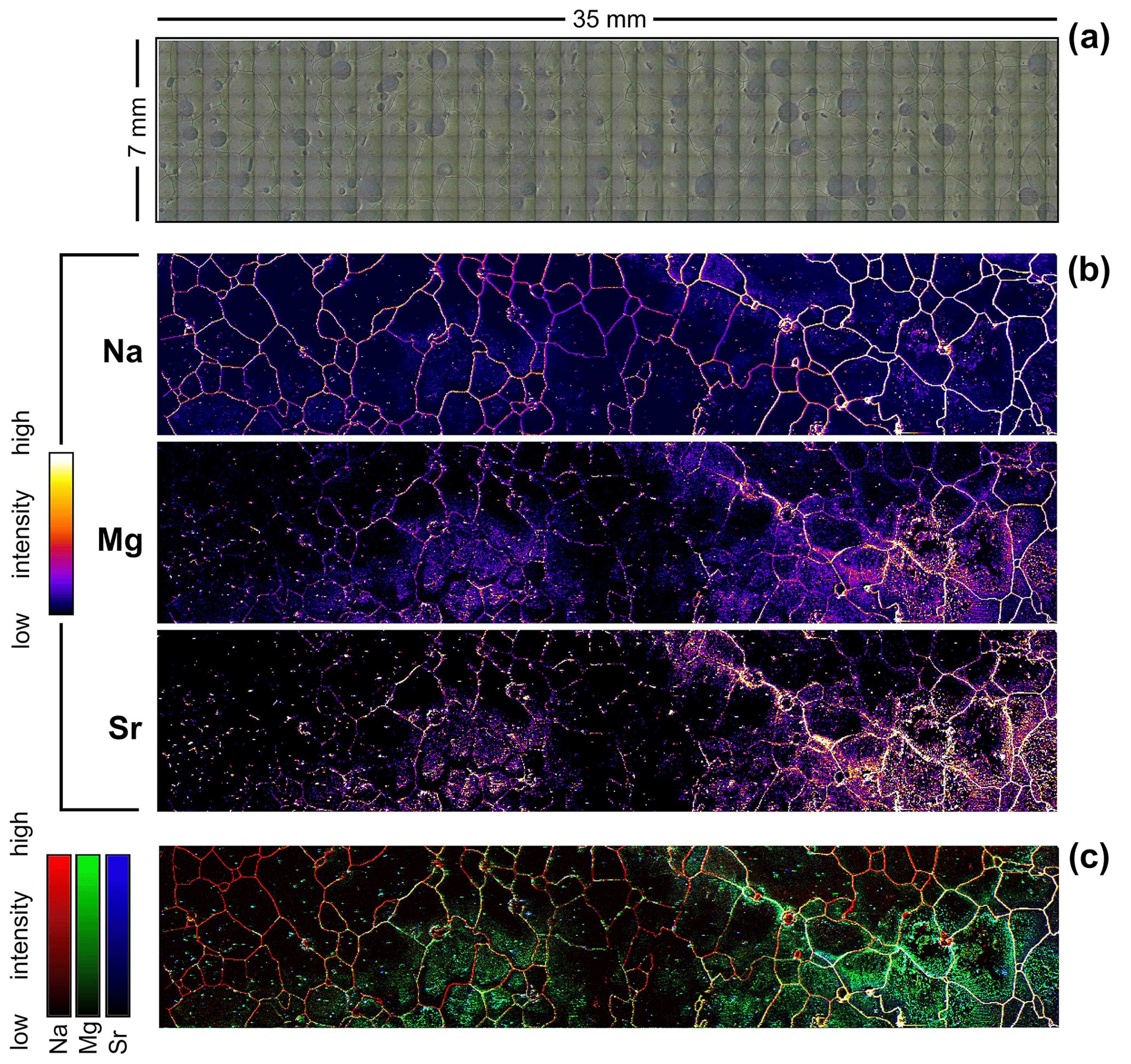
Figure 3EPICA Dome C 1065 sample from MIS 2. Panel (a) shows an optical image; panel (b) elemental maps of Na, Mg and Sr, respectively, from the same area; (c) composite RGB map of the three elements. The main core axis runs from left (top) to right.
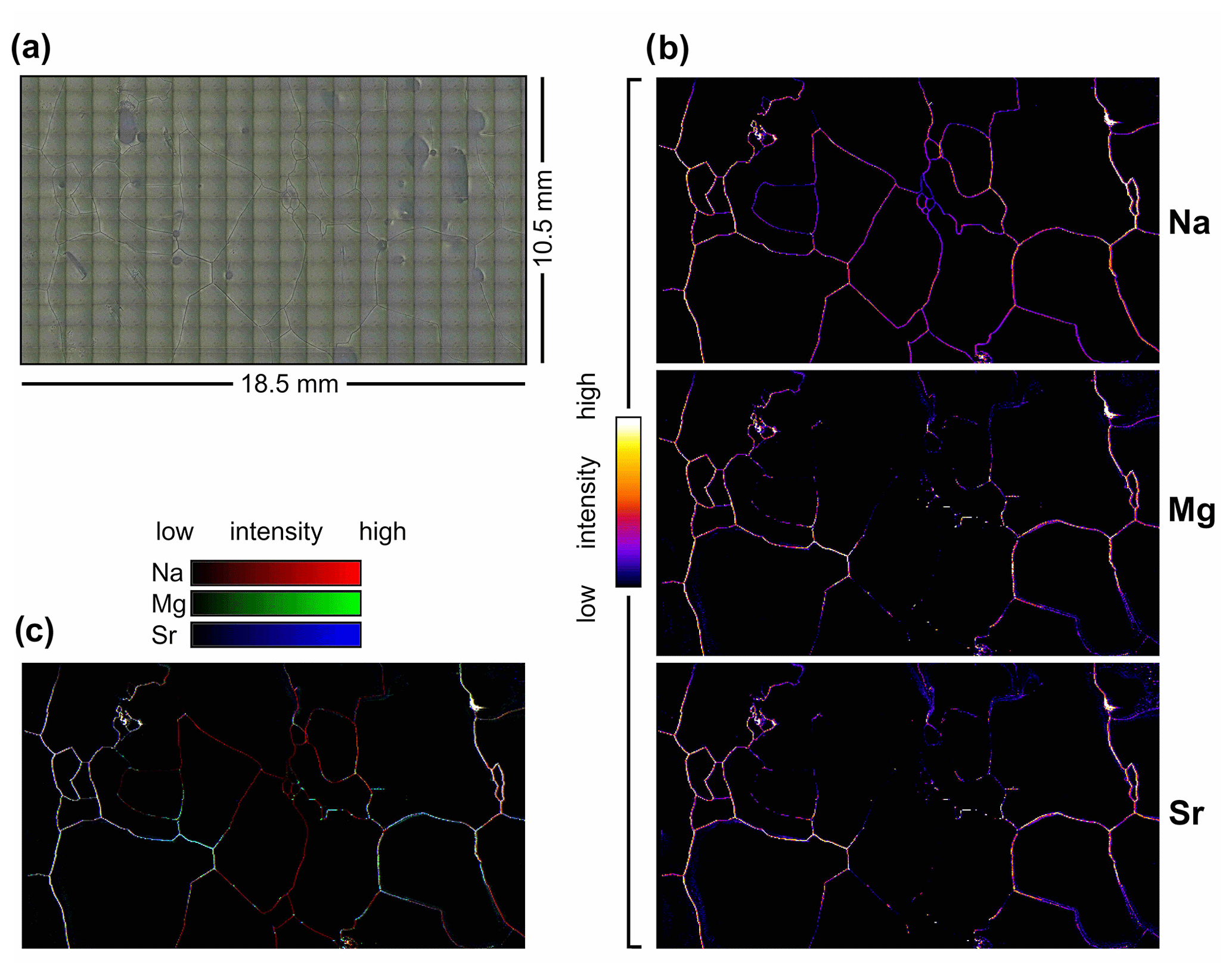
Figure 4EPICA Dome C 3092 sample from MIS 5.5. Panel (a) shows an optical image; panel (b) elemental maps of Na, Mg and Sr, respectively, in the same area; (c) composite RGB map of the three elements. The main core axis runs from left (top) to right.
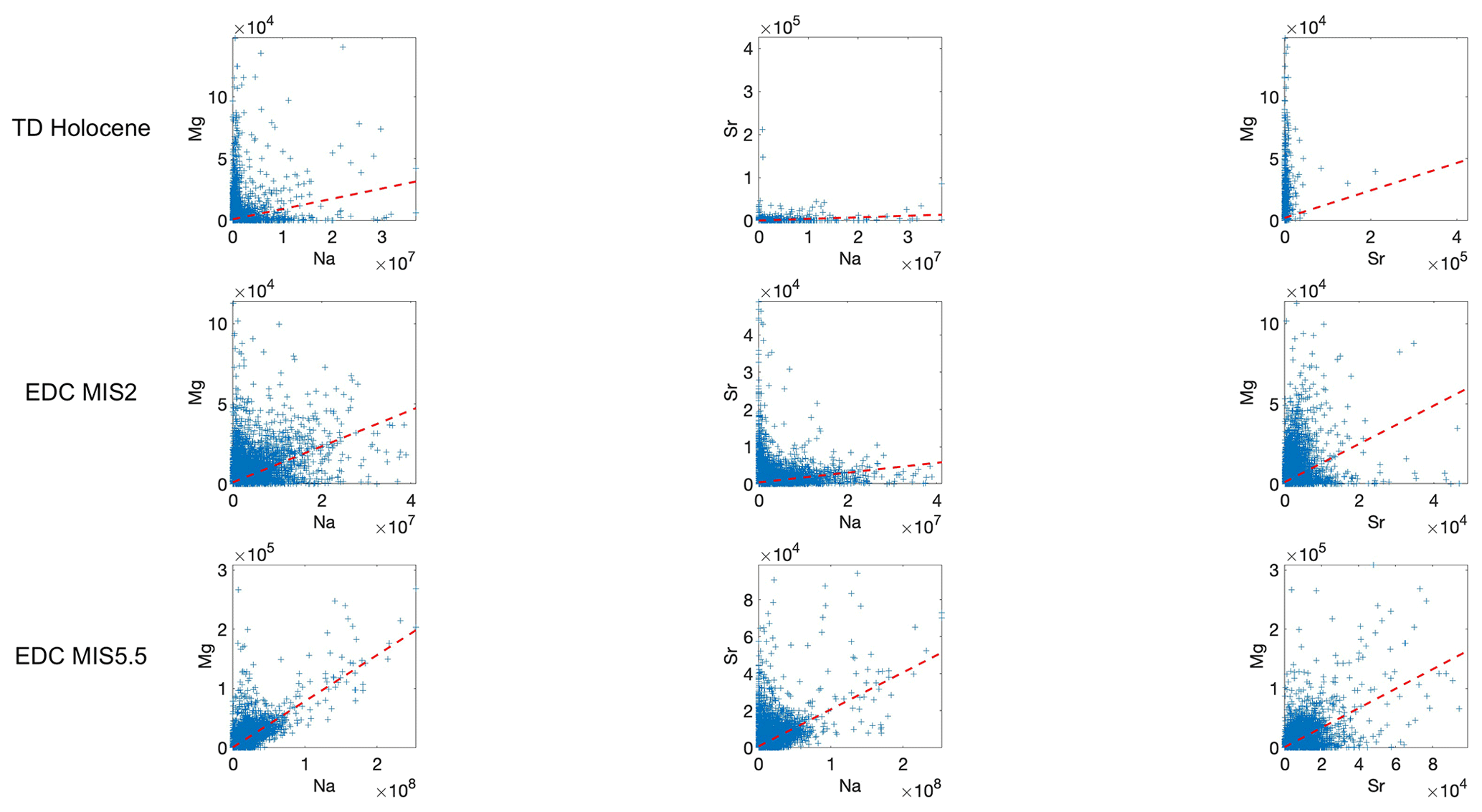
Table 2Elemental co-localization analysis using Pearson's correlation coefficient (PC), Spearman's rank coefficient (SRC) and the intensity correlation quotient (ICQ). Values in parentheses refer to results after discarding the 0.5 and 99.5 percentiles (see text).
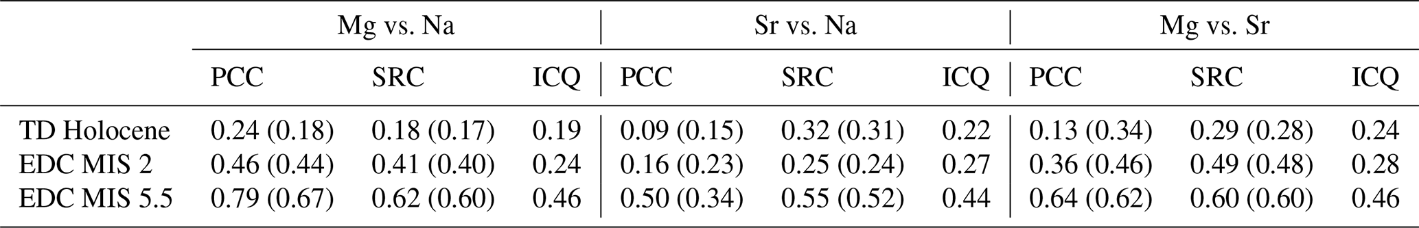
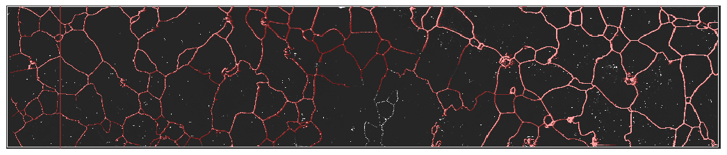
Figure 6Exemplary results of the watershed algorithm used in HDIP for Na map segmentation of the MIS 2 sample. The red markup is used to classify pixels belonging to grain boundaries. The complement is associated with grain interiors. Note how a small portion in the lower center part was missed by the semi-automated procedure due to a lack of coherency in the Na–grain boundary association. The vertical red stripe on the left image side is an artifact from figure creation.
Table 3Results from basic statistics after image segmentation into grain boundaries and grain interiors. Note that Na, Mg and Sr are intensities in counts, whereas , and are reported as elemental ratios (see text).
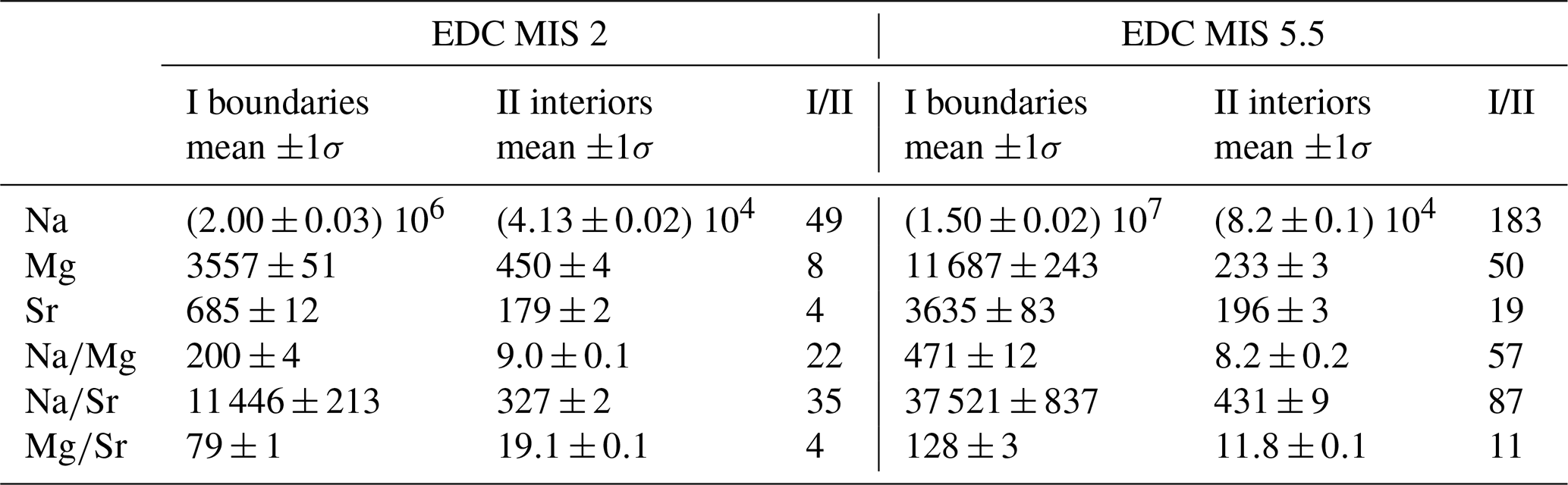
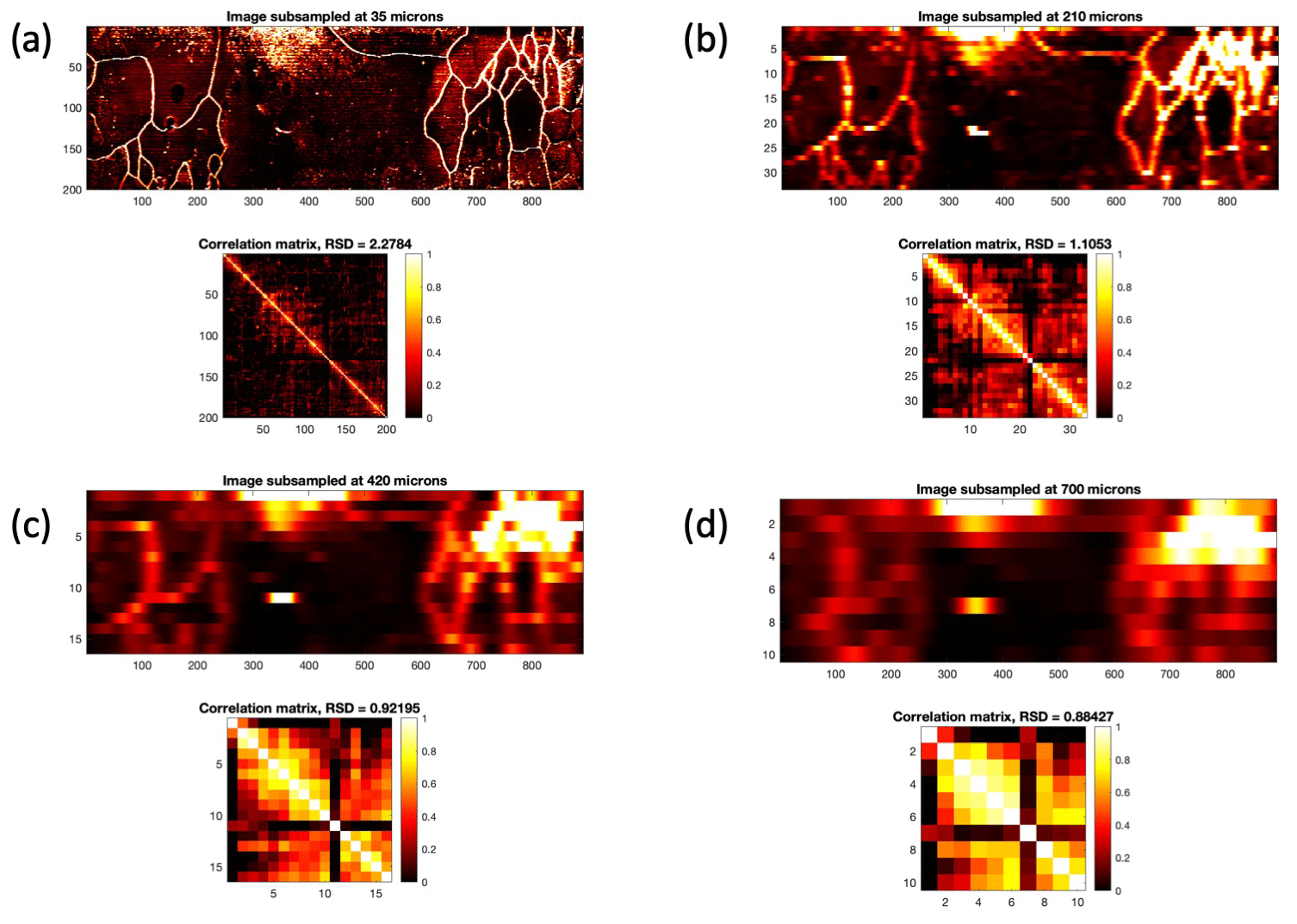
Figure 7Example images illustrating the effect of decreasing the spatial resolution of the original image (a) in 35 µm steps in the vertical and horizontal direction (see text). The correlation matrix is calculated from all lines in the sub-sampled images, together with its relative standard deviation (RSD). Shown here are results for the TD Holocene Na image, at steps of 210, 420 and 700 µm, in panels (b–d), respectively.
3.1 Basic elemental maps in comparison with optical images
The elemental intensity distribution maps obtained are shown in Figs. 2, 3 and 4, together with the optical images of the corresponding sample surface. All three analytes generally show sufficiently high signalnoise ratios. The three sets of maps show clear differences but are composed of similarly basic features. If sorted by increasing spatial extent, the basic features are the following: (i) individual bright spots, typically comprising of just a few clustered bright pixels, (ii) a network of lines, especially dominant for the Na maps, (iii) millimeter-scale differences in the intensity, with some parts of the images being distinctly lower in intensity compared to the others. Comparison with the optical images clearly shows that the network of high-intensity lines can be associated with the location of grain boundaries. For the individual bright spots, candidates are dust particles and micro-inclusions; however finding a clear association with optical features is generally difficult. In all maps, Mg and Sr show a certain degree of similarity in spatial distribution but clear differences with Na. Going into more detail, the main differences and observations between the maps/images are as follows:
-
Talos Dome, Holocene (Fig. 2). High Na intensities track the grain boundaries, while Mg and Sr have only a minor association with them. Mg and Sr show generally more evenly distributed intensities with occasional bright spots and a bright stripe within the left center half of the map showing for all elements. Notably, the latter has no clear counterpart in the optical image.
-
EPICA Dome C, MIS 2 (Fig. 3). The sample is characterized by comparatively smaller grains, as expected for a glacial period (Gow et al., 1997; Thorsteinsson et al., 1997). Bright spots are abundant for all elements. The association of network lines with grain boundaries is again most clear for Na but also found in some regions for Mg and Sr. The latter also show high intensities in some grain interiors. Intensities are generally lower in the center and towards the left-hand edge of the map.
-
EPICA Dome C, MIS 5.5 (Fig. 4). This sample stands out by showing a high degree of localization at grain boundaries for all elements. In the grain interiors, Mg and Sr occasionally show elevated intensities at locations close to the grain boundaries. Bright spots are almost completely absent.
3.2 Impurity localization and co-localization analysis
It is important to note that the focus here lies in a relative comparison of the degree of co-localization between the elements and optically visible features; this is not intended as an accurate quantification of the co-localization. To this end, imaging the localization of impurities does not require a fully quantitative method, although recent advances have been made creating matrix-matched calibrations for LA-ICP-MS with artificial ice standards (Della Lunga et al., 2017). Basic co-localization analysis was performed in order to further investigate differences in Na maps with respect to Mg and Sr, and to detect potentially minor differences in Mg and Sr signal distributions. As a first step in visual co-localization, a simple overlay composite image of the different elemental maps is included in Figs. 2, 3 and 4. In the composite, each individual map is represented by a separate color channel, using red, green and blue for Na, Mg and Sr, respectively. This means that co-localized Na and Mg (green and red) will result in yellow hot spots, whereas white areas represent all elements co-localized together. A preliminary visual analysis of the composite map already suggests that not all bright spots are co-localized, especially for Fig. 2 (MIS 2) where single channel bright spots stand out abundantly. However, the visual overlay has its limitations regarding analyzing co-localizations. Differences in absolute signal intensity and signalnoise ratio can subdue or mask co-localization. The composite images in Figs. 2, 3 and 4 with each element in a separate color channel are thus considered only as a starting point.
For further comparison of the degree of co-localization, the matrices of intensity values that underlie the images shown in Figs. 2 and 3 and 4 were used to make scatter plots for each pair of elements. As becomes evident from Fig. 5, the intensities for Mg and Sr are generally similar, while Na intensities can be higher by several orders of magnitude. This difference can be explained by higher Na concentrations paired with a higher (absolute) instrumental sensitivity for the element. The scatterplots also indicate the almost absent co-localization in the TD Holocene image, showing signs of mutual exclusions (values extremely close to one axis). For EDC MIS 2 some correlation emerges but becomes most evident for EDC MIS 5.5.
Several metrics to quantify co-localization in images, e.g., similar those used for tissue analysis with fluorescence microscopy, have been established in the literature (Bolte and Cordelières, 2006). For intensity correlation coefficient-based analyses, the Pearson's correlation coefficient (PCC), the Spearman's rank coefficient (SRC) and the intensity correlation quotient (ICQ) were considered in this work, since they are superior in many cases over the Mander's overlap coefficient (Adler and Parmryd, 2010). The SRC equals the PCC applied to ranked data, in which case the relative amplification in Na intensities should not play a role. Since PCC and SRC can be sensitive to thresholding, the robustness of the values was checked against results obtained after discarding the 0.5 and 99.5 percentiles of the data. Compared to PCC and SRC, the ICQ has a higher sensitivity to midrange pixels (Adler and Parmryd, 2010). It only considers the sign, or respectively whether each of the two intensities are above or below their respective mean intensity, by constructing its ranges from −0.5 to 0.5, denoting negative and positive correlation, respectively (Li et al., 2004). The ICQ was calculated with the public domain tool named JACoP (Bolte and Cordelières, 2006) available for the software imageJ after converting the maps to grayscale.
The results of co-localization analysis are summarized in Table 2. Regarding the comparison between the three samples, the PCC, SRC and ICQ results substantiate the previously noted findings from a visual analysis. No clear evidence for inter-elemental correlation is found for the TD Holocene sample. In contrast, correlation is generally strongest for the EDC MIS 5.5 sample, with the highest PCC score of 0.79 for Na and Mg. The EDC MIS 2 sample presents an intermediate case.
3.3 An exploration of analysis by image segmentation
The fact that Na shows a clear signal at all grain boundaries allows image segmentation based solely on the LA-ICP-MS images to be performed, without using the optical mosaics which lack sufficient image quality. Segmentation means the extraction of the positions of all the pixels in the image that are part of the grain boundary signal. This can be performed using a “watershed” algorithm, a technique commonly used in image processing for segmentation (Vincent and Soille, 1991). In this approach the gray scale of the image is regarded as a topographic map, with the elevation being represented by the pixel intensity. The task then is to find the “crest lines” in the topographic map. This analysis was performed semi-automatically using a watershed-type algorithm within the software HDIP: bright pixels in the grain boundaries are selected manually as a starting point, and the flood tolerance parameter is increased iteratively until the connecting network lines are selected. This procedure is repeated until the grain boundaries of the image have been selected as a “region of interest”. The result is two sub-sets of pixels in the image: pixels associated either with a grain boundary or grain interior (Fig. 6). Then, basic statistics are performed on the two subsets individually. Table 3 summarizes the results for the MIS 2 and MIS 5.5 samples.
Based on the coarse assumption that ablation differences between the glass reference materials and the ice samples can be neglected, the intensity ratios can be converted into elemental (mass) ratios using the NIST SRM 612 as a reference (Longerich et al., 1996; Jochum et al., 2011). Following this approach (Della Lunga et al., 2014), , and are converted accordingly in Table 3.
The ratios reveal that the relative enrichment at grain boundaries is generally highest for Na, between 3–6 times higher than for Mg and around 10 times higher than for Sr. Next, the relative enrichment at grain boundaries is 3–5 times higher in MIS 5.5 compared to MIS 2. The relatively higher enrichment of Na at grain boundaries translates into corresponding high values of and . The ratio is also increased at grain boundaries, although to a lesser extent than the ratios including Na.
3.4 Spatial significance of single line profiles
In order to simulate how the spatial impurity distribution would appear in coarser-resolution LA-ICP-MS elemental imaging, the 35 µm resolution images are sub-sampled in longitudinal (along the scan, i.e., left to right) and transversal (perpendicular to the scan) direction. The transversal sub-sampling is primarily simulating using a larger spot size, whereas the decrease in longitudinal direction additionally corresponds to longer washout times. The rows of the original images are averaged stepwise in increments of one line, making the transversal resolution decrease in 35 µm steps. To decrease the longitudinal resolution by approximately the same step, Gaussian filtering is applied subsequently to each line with a kernel size adjusted accordingly. Using a Gaussian filter along the scan direction in each line mimics the combined effects of increasing washout time and the moving laser (firing at a fixed repetition rate). This is not needed in the transversal direction since individual lines are essentially independent samples. In order to assess the spatial significance of a single longitudinal line, all lines in the image are correlated against each other. The correlation matrix (using the PCC) between all lines in the image is thus symmetric and should be perfectly white (i.e., equal to unity) in case of identical lines. This ideal case would correspond to perfect spatial significance, because it would be irrelevant at which position the individual line profile is measured. The actual images do not fulfill this ideal case. The relative standard deviation (RSD) of the correlation matrix entries is reported to quantify the degree of inhomogeneity.
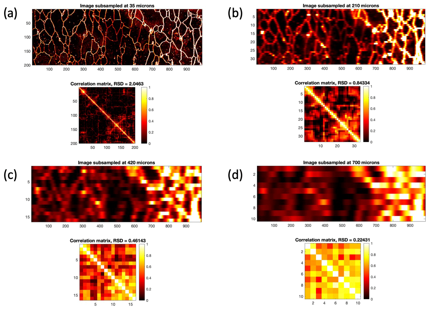
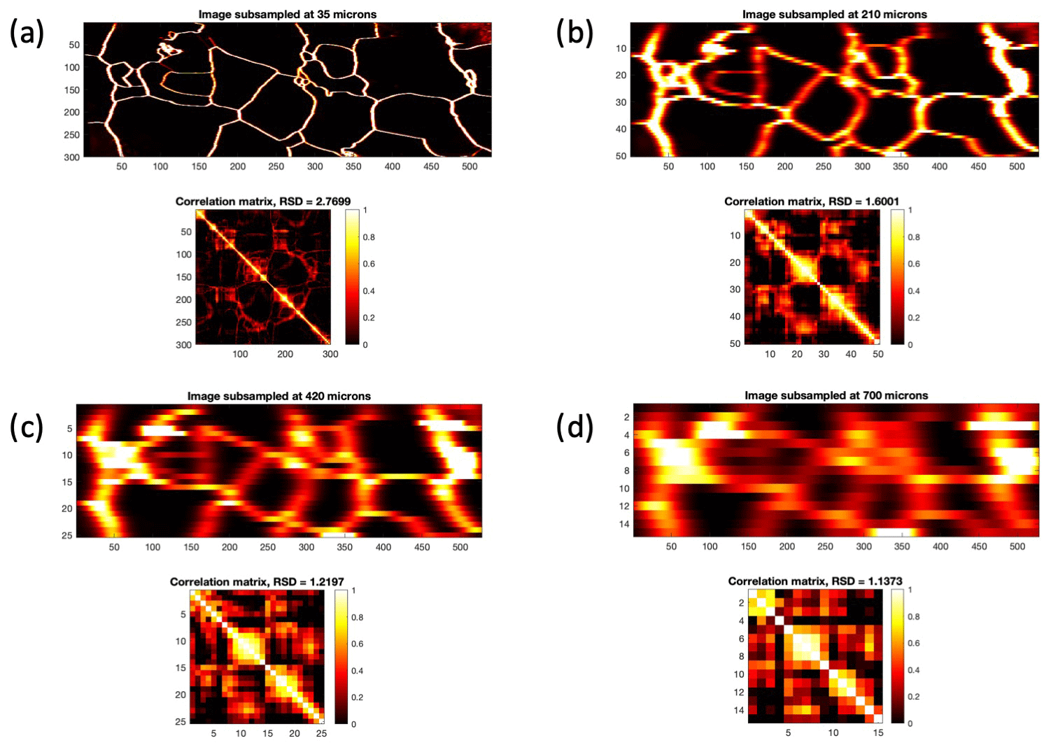
Results are shown here for Na, since it has the strongest imprint at the grain boundaries. Results for Mg are in the Supplement, and are almost identical to the Sr results (hence not shown). Figures 7, 8 and 9 show the results for the TD Holocene, EDC MIS 2 and EDC MIS 5.5 image, respectively. Shown are the original image and three examples of the evolution at 35 µm steps, corresponding to a spatial resolution of 210, 420 and 700 µm, respectively. It becomes evident that the signal of the small-scale bright spots has vanished at 210 µm, while the majority of the grain boundary remains visible and traceable throughout the images. The presence of the spatially coherent signal corresponding to the grain boundaries is related to the grain size: large grains remain visible even at 420 µm, while comparatively smaller grains cannot be distinguished anymore. This becomes especially clear when comparing the 420 µm images of EDC MIS 2 and EDC MIS 5.5, Figs. 8 and 9, respectively. At a scale of 700 µm, the TD Holocene and EDC MIS 2 images resemble mostly the large-scale intensity gradients. At this point, a high degree of correlation among single lines is achieved. This means that the obtained signal is largely independent of the positioning of the line profile perpendicular to the scan direction. Notably, this situation is different for the EDC MIS 5.5 images, which is comprised of comparatively large grains. Regarding Mg, a comparable degree of homogeneity as seen for Na is achieved at the exemplary intervals of 210, 420 and 700 µm shown here, as indicated by similar relative standard deviation (RSD) values (Supplement).
The results are discussed in view of the two-fold exploration into the use of the LA-ICP-MS imaging technique to reveal (i) 2-D maps of the impurity distribution in relation to the grain boundary network and (ii) constraints arising for the interpretation of line profiles as high-resolution stratigraphic signals, allowing the adaption of the experimental design accordingly.
4.1 Impurity localization and grain boundary network
The two EDC images not only corroborate the previously observed correlation between high Na intensity and the locations of grain boundaries in the TD Holocene sample (Bohleber et al., 2020) but also extend the approach to samples from core sections with very different physical and chemical properties. The three maps exhibit clear differences in their general features and the degree of impurity localization at grain boundaries, the latter generally increasing from Holocene–MIS 2–MIS 5.5 for all elements. This difference argues against sample contamination or that surface changes play a dominant role in the 2-D impurity maps, which arguably would make all samples look similar. The demonstrated reproducibility of the images shows that these are not artifacts (Bohleber et al., 2020). The rigorous ice core decontamination protocols used have been proven adequate for LA-ICP-MS ice core analysis (Della Lunga et al., 2014, 2017). Notably, the general tendency of Na and, to a lesser extent, Mg to localize at grain boundaries is consistent with LA-ICP-MS impurity mapping of ice samples of Greenland ice cores. However, prior to the advent of the LA-ICP-MS imaging technique, elemental maps had to be acquired using arrays (grids) of laser spots with spot sizes larger than 100 µm, followed by spatial interpolation. Consequently, this method faced limitations regarding investigations on impurity localization at grain boundaries (Della Lunga et al., 2014, 2017). In this context, the artifact-free images generated at 35 µm resolution and without further interpolation provide a significant step forward.
Considering the comparison of the two EDC samples from MIS 2 and MIS 5.5 in more detail, the in-grain signals, distributed intensity and individual bright spots, stand out in the MIS 2 maps but are almost entirely absent in MIS 5.5. Assuming a relationship between bright spots and micro-inclusions or dust-related particles, this difference in map features between the glacial and interglacial sample is consistent with the macroscopic chemistry: glacial impurity (including dust) concentrations are generally up to several orders of magnitude higher than the interglacial ones (e.g., Fischer et al., 2007; Lambert et al., 2008). The known smaller average crystal area in glacial samples is also observed, especially through the Na map. In the MIS 5.5 sample Mg and Sr are also located predominantly at grain boundaries, with only minor signals from the grain interiors.
The fact that the enrichment at grain boundaries is generally highest for Na, followed by Mg and Sr, suggests that on the micrometer scale, differences in the interaction with the grain boundary network exist between these elements and in the ice from different climatic periods. Mg may be related to sea salt as well as terrestrial dust (Legrand and Mayewski, 1997). However, based on the LA-ICP-MS images, Mg shows a clear preference neither for Na (related mostly to sea salt) nor for Sr (a tentative substitute for terrestrial dust sources more commonly investigated through Ca). The ratio also shows significant enrichment in Na at the grain boundaries (Table 3). However, it seems worth noting that in the grain interior the is within the range typical for sea salt (e.g., Mouri et al., 1993), warranting further investigation.
When considering the Na enrichment at the grain boundaries, using a simplified view would mean that with grains growing over time, the comparatively mobile (e.g., soluble Na) species are more easily collected at the grain boundaries compared to the less mobile species such as the insoluble particulate fraction. This is simplified because particulate inclusions may also inhibit grain boundary growth (e.g., through “pinning of” or “dragging with” grain boundaries). This process could also result in localization of particulate impurities at boundaries (Faria et al., 2014b; Stoll et al., 2021). It is evident that only limited generalized conclusions can be drawn from the small-sized images. Accordingly, it is not intended here to discuss in detail the different behavior of chemical impurities in relation to their mobility and insoluble fractions.
However, in the future, with multi-elemental images, such an analysis may become possible. Imaging the localization of impurities does not require a fully quantitative method for this purpose. As an additional indicator, the ratio of intensities, either between boundaries and interiors, or between two elemental species, can also be investigated without calibration. Since LA-ICP-MS measures the total impurity amount, and thus cannot directly distinguish soluble and insoluble fractions, a broader spectrum of elements could serve to identify impurities associated with a specific aerosol based on their glacio-chemical signature (Oyabu et al., 2020).
Until images comprising of a larger number of elements become available, introducing image analysis techniques can provide an alternative to overcoming such limitations. This approach was explored here to compare intra-grain vs. in-grain signals. It is worth pointing out that this type of analysis using image segmentation was performed as a post-processing step and did not require a separate experimental design. Experiments aimed at comparison of intra-grain vs. in-grain distributions were previously performed with LA-ICP-MS but required manual tracking of the grain boundaries with the laser scan (Beers et al., 2020; Kerch, 2016). It becomes clear that the new LA-ICP-MS imaging technique can offer important insights into the ice stratigraphy on the micrometer scale and that special merit comes from introducing techniques for image analysis and applying them to investigations of the chemical images. Future efforts in combining image analysis from both techniques in an automated way for even larger images seem highly intriguing in this context (Bohleber et al., 2021b).
LA-ICP-MS chemical imaging may become especially used when investigating the conditions in very deep ice, particularly when looking at impurity diffusion and post-depositional chemical reactions. The localization of impurities at grain boundaries and triple junctions is a prerequisite for their potential migration along the ice vein network (Rempel et al., 2001; Ng, 2021). Imaging of Mg could also provide additional insights in the anomalous signals occurring in the EDC chemical records below 2800 m, in particular when combined with the analysis of S (or chemical substitutes for sulfate) (Traversi et al., 2009). In the future, a meaningful comparison with elemental concentrations and ratios from other macroscopic techniques, such as continuous flow analysis, calls for larger, centimeter-sized areas. Regarding an inter-method comparison over smaller areas, the comparison with cryo-Raman analysis or synchrotron radiation techniques (Baccolo et al., 2018) may provide added value for the investigation of impurity localization, in particular micro-inclusions and dust. In contrast to the findings of this present work, cryo-Raman performed on the EPICA DML core for MIS 6 and MIS 5e detected no significant relationship between micro-inclusions and grain boundaries, and it lacked a signal for the dissolved impurities (Eichler et al., 2019). Although major challenges may arise due to methodological differences, a direct comparison between LA-ICP-MS and these two techniques seems a worthwhile future goal (Stoll et al., 2021).
4.2 Spatial significance of line profiles and future experimental design
In addition to investigation of impurity localization, LA-ICP-MS ice core analysis is of special interest for probing extremely thin stratigraphic layers as high-resolution paleoclimate records. For ice cores from coastal Antarctica, a resolution of a few hundred micrometers can offer the detection of annual layers even in deeper samples (Haines et al., 2016). When comparing LA-ICP-MS results with those from continuous flow analysis, further smoothing is commonly applied to the LA-ICP-MS signals prior interpretation (Della Lunga et al., 2017; Bohleber et al., 2018).
At a resolution of 35 µm, these results demonstrate that crystal features such as grain boundaries determine the high-frequency signal components in single line profiles. This means that signals obtained from line profiles will be greatly influenced by their position on the surface, i.e., transversal to the core axis and scan direction. In contrast to this, the central hypothesis of ice core analysis is that the original stratigraphy resulting from paleoclimatic variability should produce signals that are not a function of the transversal position of the scan line. This can be overcome by measuring multiple parallel scan lines, which should have a high degree of shared signal and thus have a higher spatial significance. Notably, this ideal case may already start to be flawed once so-called micro-folds in the ice (Svensson et al., 2005; Jansen et al., 2016) start to appear.
This raises the following problem: on the one hand, when investigating paleoclimatic signals on a millimeter to micrometer scale, the measurement of single line profiles along the main core axis is preferred in order to avoid the comparatively time- and resource-intensive nature of the imaging technique. But on the other hand, only imaging can provide the required detail regarding the signal imprints arising from ice crystal features such as grain boundaries. This means that an experimental design based on imaging should first set the choice of spatial scale (measurement resolution), so that the spatial coherence is maximized and the grain boundary imprint minimized.
The results from simulating coarser-resolution images show how this can be achieved based on the high-resolution images. For the TD Holocene and EDC MIS 2 image a resolution of 400–700 µm can be sufficient to achieve transversal signal coherence. This is consistent with the need to further reduce the resolution in previous studies using spot sizes of around 200 µm (Sneed et al., 2015; Della Lunga et al., 2017; Spaulding et al., 2017; Bohleber et al., 2018). The instance of the EDC MIS 5.5 image shows that this range is not a generally applicable value, however: for the larger grains the signals remain substantially heterogenous in the transversal direction.
It is clear that maximizing spatial coherence will immediately depend on the following: (i) the degree of localization of an impurity species at the grain boundaries and (ii) the average size of the grains with respect to the stratigraphic layering of interest. Both can be taken into account with the 2-D impurity imaging technique. Considering an average grain radius of around 5–6 mm in the deeper sections of the EDC ice core (EPICA Community Members, 2004), the required size of the maps should be substantially larger than the present ones.
The increase in map size is a considerable yet solvable technical and practical challenge. Even with the high scan speed employed here, the recording of a 7×10.5 mm image requires 200 parallel scan lines at a 35 mm spot size, corresponding to 1.8 million individual laser shots fired. With unidirectional measurements the imaging takes around 2.5 h, although imaging time can be reduced by about 30 % if scanning in a bidirectional mode. The latest technological developments in LA-ICP-MS imaging promise further advancement in speed through faster washout and higher repetition rate lasers (Šala et al., 2020; Van Acker et al., 2021). Regarding stratigraphic line scans with LA-ICP-MS, the already developed large cryogenic chambers can eliminate the need for preparing centimeter-sized samples (Sneed et al., 2015). If combined with the scan speed achieved in the present method, the line scan of a 55 cm core section would be completed in under 10 min. In this framework, the present study clearly demonstrates the merit of the LA-ICP-MS imaging technique both for studying impurity localization and setting the experimental design for stratigraphic investigations. The imaging approach should hence be integrated in future efforts in ice core analysis by LA-ICP-MS.
Through the integration of state-of-the-art imaging techniques, LA-ICP-MS ice core analysis has taken the step from 1-D into 2-D. The next level in LA-ICP-MS ice core analysis now offers scan speeds increased by 1 order of magnitude for single line profiles and the ability to map the localization of impurities at a high spatial resolution (35 µm). The present work has demonstrated the new potential for investigating the location of impurities and for improving the interpretation of single line profiles considering imprints from ice crystal features. Two-dimensional chemical imaging with LA-ICP-MS showed distinct differences among glacial and interglacial samples of the Talos Dome and EPICA Dome C ice cores from central Antarctica. The images reveal that grain boundaries coincide with high intensities of Na for all samples. In the Talos Dome Holocene sample and the glacial sample from EPICA Dome C, Mg and Sr are presented also in the grain interiors. The interglacial sample from MIS 5.5 shows all elements predominantly at grain boundaries. This finding is corroborated by introducing image segmentation techniques to separately quantify in-grain vs. intra-grain intensities as well as their ratios. Simulations of coarser-resolution experiments show that the spatial significance of a single line profile increases as the imprint of grain boundaries weakens at a coarser resolution. This allows settings to be adapted to be specifically fit for purpose, e.g., to avoid misinterpretation of ultra-fine-resolution signals in the presence of ice crystal imprints. An immediate future target is imaging over larger areas to increase their spatial significance, in particular for investigations in deep ice with centimeter-sized grains. In this regard, the present findings have clearly demonstrated the merit of driving forward the LA-ICP-MS ice core imaging technique.
The underlying datasets can be found at the Pangaea repository: https://doi.pangaea.de/10.1594/PANGAEA.933333 (Bohleber et al., 2021a).
The supplement related to this article is available online at: https://doi.org/10.5194/tc-15-3523-2021-supplement.
PB conducted the measurements with help of MR. The experimental design was developed by PB with the help of MR, MS and CB. PB wrote an initial version of the manuscript. All authors contributed to the discussion of the results and the final version of the manuscript.
The authors declare that they have no conflict of interest.
Publisher's note: Copernicus Publications remains neutral with regard to jurisdictional claims in published maps and institutional affiliations.
This article is part of the special issue “Oldest Ice: finding and interpreting climate proxies in ice older than 700 000 years (TC/CP/ESSD inter-journal SI)”. It is not associated with a conference.
The authors thank Ciprian Stremtan and Stijn van Malderen for their technical support. Likewise we thank Alessandro Bonetto for support in the laboratory, Luca Fiorini for assistance with the spatial significance experiments and Warren Cairns for language editing. Marcello Pelillo, Kaleem Siddiqi and Sebastiano Vascon are gratefully acknowledged for helpful discussions on image analysis. Pascal Bohleber gratefully acknowledges funding from the European Union's Horizon 2020 research and innovation program under the Marie Skłodowska-Curie grant agreement no. 790280. Martin Šala acknowledges support from the Slovenian Research Agency (ARRS), contract number P1-0034. ELGA LabWater is acknowledged for providing the PURELAB Option-Q and Ultra Analytic systems, which produced the ultrapure water used for cleaning and decontamination. This publication was generated in the frame of Beyond EPICA. The project has received funding from the European Union's Horizon 2020 research and innovation program under grant agreement no. 815384 (Oldest Ice Core). It is supported by national partners and funding agencies in Belgium, Denmark, France, Germany, Italy, Norway, Sweden, Switzerland, the Netherlands and the UK. Logistic support is mainly provided by PNRA and IPEV through the Concordia Station system. The opinions expressed and arguments employed herein do not necessarily reflect the official views of the European Union funding agency or other national funding bodies. This is Beyond EPICA publication number 19. The Talos Dome Ice Core Project (TALDICE), a joint European program led by Italy, is funded by national contributions from Italy, France, Germany, Switzerland and the UK. This is TALDICE publication 61.
This research has been supported by the H2020 Marie Skłodowska-Curie Actions (grant no. 790280), the H2020 Environment (grant no. 815384), and the Slovenian Research Agency (ARRS) (contract no. P1-0034).
This paper was edited by Joel Savarino and reviewed by David M. Chew and one anonymous referee.
Adler, J. and Parmryd, I.: Quantifying colocalization by correlation: the Pearson correlation coefficient is superior to the Mander's overlap coefficient, Cytom. Part A, 77, 733–742, https://doi.org/10.1002/cyto.a.20896, 2010. a, b
Ahn, J., Wahlen, M., Deck, B. L., Brook, E. J., Mayewski, P. A., Taylor, K. C., e and White, J. W.: A record of atmospheric CO2 during the last 40,000 years from the Siple Dome, Antarctica ice core, J. Geophys. Res.-Atmos., 109, D13305, https://doi.org/10.1029/2003JD004415, 2004. a
Baccolo, G., Cibin, G., Delmonte, B., Hampai, D., Marcelli, A., Di Stefano, E., Macis, S., and Maggi, V.: The contribution of synchrotron light for the characterization of atmospheric mineral dust in deep ice cores: Preliminary results from the Talos Dome ice core (East Antarctica), Condens. Matter, 3, 25, https://doi.org/10.3390/condmat3030025, 2018. a
Barnes, P. R. and Wolff, E. W.: Distribution of soluble impurities in cold glacial ice, J. Glaciol., 50, 311–324, https://doi.org/10.3189/172756504781829918, 2004. a
Barnes, P. R., Wolff, E. W., Mallard, D. C., and Mader, H. M.: SEM studies of the morphology and chemistry of polar ice, Microsc. Res. Techniq., 62, 62–69, https://doi.org/10.1002/jemt.10385, 2003. a
Beers, T. M., Sneed, S. B., Mayewski, P. A., Kurbatov, A. V., and Handley, M. J.: Triple Junction and Grain Boundary Influences on Climate Signals in Polar Ice, arXiv [preprint], arXiv:2005.14268 2020. a, b
Bohleber, P., Erhardt, T., Spaulding, N., Hoffmann, H., Fischer, H., and Mayewski, P.: Temperature and mineral dust variability recorded in two low-accumulation Alpine ice cores over the last millennium, Clim. Past, 14, 21–37, https://doi.org/10.5194/cp-14-21-2018, 2018. a, b
Bohleber, P., Roman, M., Šala, M., and Barbante, C.: Imaging the impurity distribution in glacier ice cores with LA-ICP-MS, J. Anal. Atom. Spectrom., 35, 2204–2212, https://doi.org/10.1039/D0JA00170H, 2020. a, b, c, d, e, f
Bohleber, P., Roman, M., Šala, M., Delmonte, B., Stenni, B., and Barbante, C.: Chemical impurity distribtion (Na, Mg, Sr) in the EPICA Dome C ice core bags 1065 and 3092 and Talos Dome ice core bag 375-B1 obtained from 2D imaging with LA-ICP-MS, PANGAEA [data set], https://doi.pangaea.de/10.1594/PANGAEA.933333, 2021a. a
Bohleber, P., Roman, M., Barbante, C., Vascon, S., Siddiqi, K., and Pelillo, M.: Ice Core Science Meets Computer Vision: Challenges and Perspectives, Front. Comput. Sci., 3, 54, https://doi.org/10.3389/fcomp.2021.690276, 2021b. a
Bolte, S. and Cordelières, F. P.: A guided tour into subcellular colocalization analysis in light microscopy, J. Microsc., 224, 213–232, https://doi.org/10.1111/j.1365-2818.2006.01706.x, 2006. a, b
Brook, E. J., Wolff, E., Dahl-Jensen, D., Fischer, H., and Steig, E. J.: The future of ice coring: international partnerships in ice core sciences (IPICS), Pages News, 14, 6–10, 2006. a
Dahl-Jensen, D., Thorsteinsson, T., Alley, R., and Shoji, H.: Flow properties of the ice from the Greenland Ice Core Project ice core: the reason for folds?, J. Geophys. Res.-Oceans, 102, 26831–26840, https://doi.org/10.1029/97JC01266, 1997. a
Della Lunga, D., Müller, W., Rasmussen, S. O., and Svensson, A.: Location of cation impurities in NGRIP deep ice revealed by cryo-cell UV-laser-ablation ICPMS, J. Glaciol., 60, 970–988, https://doi.org/10.3189/2014JoG13J199, 2014. a, b, c, d, e
Della Lunga, D., Müller, W., Rasmussen, S. O., Svensson, A., and Vallelonga, P.: Calibrated cryo-cell UV-LA-ICPMS elemental concentrations from the NGRIP ice core reveal abrupt, sub-annual variability in dust across the GI-21.2 interstadial period, The Cryosphere, 11, 1297–1309, https://doi.org/10.5194/tc-11-1297-2017, 2017. a, b, c, d, e, f, g, h, i, j, k
Eichler, J., Kleitz, I., Bayer-Giraldi, M., Jansen, D., Kipfstuhl, S., Shigeyama, W., Weikusat, C., and Weikusat, I.: Location and distribution of micro-inclusions in the EDML and NEEM ice cores using optical microscopy and in situ Raman spectroscopy, The Cryosphere, 11, 1075–1090, https://doi.org/10.5194/tc-11-1075-2017, 2017. a
Eichler, J., Weikusat, C., Wegner, A., Twarloh, B., Behrens, M., Fischer, H., Hörhold, M., Jansen, D., Kipfstuhl, S., Ruth, U., Wilhelms, F., and Weikusat, I.: Impurity analysis and microstructure along the climatic transition from MIS 6 into 5e in the EDML ice core using cryo-Raman microscopy, Front. Earth Sci., 7, 20, https://doi.org/10.3389/feart.2019.00020, 2019. a
EPICA Community Members: Eight glacial cycles from an Antarctic ice core, Nature, 429, 623–628, https://doi.org/10.1038/nature02599, 2004. a, b, c
Faria, S. H., Weikusat, I., and Azuma, N.: The microstructure of polar ice. Part I: Highlights from ice core research, J. Struct. Geol., 61, 2–20, https://doi.org/10.1016/j.jsg.2013.09.010, 2014a. a
Faria, S. H., Weikusat, I., and Azuma, N.: The microstructure of polar ice. Part II: State of the art, J. Struct. Geol., 61, 21–49, https://doi.org/10.1016/j.jsg.2013.11.003, 2014b. a
Fischer, H., Siggaard-Andersen, M.-L., Ruth, U., Röthlisberger, R., and Wolff, E.: Glacial/interglacial changes in mineral dust and sea-salt records in polar ice cores: Sources, transport, and deposition, Rev. Geophys., 45, RG1002, https://doi.org/10.1029/2005RG000192, 2007. a
Fischer, H., Severinghaus, J., Brook, E., Wolff, E., Albert, M., Alemany, O., Arthern, R., Bentley, C., Blankenship, D., Chappellaz, J., Creyts, T., Dahl-Jensen, D., Dinn, M., Frezzotti, M., Fujita, S., Gallee, H., Hindmarsh, R., Hudspeth, D., Jugie, G., Kawamura, K., Lipenkov, V., Miller, H., Mulvaney, R., Parrenin, F., Pattyn, F., Ritz, C., Schwander, J., Steinhage, D., van Ommen, T., and Wilhelms, F.: Where to find 1.5 million yr old ice for the IPICS ”Oldest-Ice” ice core, Clim. Past, 9, 2489–2505, https://doi.org/10.5194/cp-9-2489-2013, 2013. a
Gow, A., Meese, D., Alley, R., Fitzpatrick, J., Anandakrishnan, S., Woods, G., and Elder, B.: Physical and structural properties of the Greenland Ice Sheet Project 2 ice core: A review, J. Geophys. Res.-Oceans, 102, 26559–26575, https://doi.org/10.1029/97JC00165, 1997. a
Haines, S. A., Mayewski, P. A., Kurbatov, A. V., Maasch, K. A., Sneed, S. B., Spaulding, N. E., Dixon, D. A., and Bohleber, P. D.: Ultra-high resolution snapshots of three multi-decadal periods in an Antarctic ice core, J. Glaciol., 62, 31–36, https://doi.org/10.1017/jog.2016.5, 2016. a, b
Iliescu, D. and Baker, I.: Effects of impurities and their redistribution during recrystallization of ice crystals, J. Glaciol., 54, 362–370, https://doi.org/10.3189/002214308784886216, 2008. a
Jansen, D., Llorens, M.-G., Westhoff, J., Steinbach, F., Kipfstuhl, S., Bons, P. D., Griera, A., and Weikusat, I.: Small-scale disturbances in the stratigraphy of the NEEM ice core: observations and numerical model simulations, The Cryosphere, 10, 359–370, https://doi.org/10.5194/tc-10-359-2016, 2016. a
Jochum, K. P., Weis, U., Stoll, B., Kuzmin, D., Yang, Q., Raczek, I., Jacob, D. E., Stracke, A., Birbaum, K., Frick, D. A., Günther, D., and Enzweiler, J.: Determination of reference values for NIST SRM 610–617 glasses following ISO guidelines, Geostand. Geoanal. Res., 35, 397–429, https://doi.org/10.1111/j.1751-908X.2011.00120.x, 2011. a
Kaufmann, P. R., Federer, U., Hutterli, M. A., Bigler, M., Schüpbach, S., Ruth, U., Schmitt, J., and Stocker, T. F.: An improved continuous flow analysis system for high-resolution field measurements on ice cores, Environ. Sci. Technol., 42, 8044–8050, https://doi.org/10.1021/es8007722, 2008. a
Kawamura, K., Nakazawa, T., Aoki, S., Sugawara, S., Fujii, Y., and Watanabe, O.: Atmospheric CO2 variations over the last three glacial'interglacial climatic cycles deduced from the Dome Fuji deep ice core, Antarctica using a wet extraction technique, Tellus B, 55, 126–137, https://doi.org/10.3402/tellusb.v55i2.16730, 2003. a
Kerch, J. K.: Crystal-orientation fabric variations on the cm-scale in cold Alpine ice: Interaction with paleo-climate proxies under deformation and implications for the interpretation of seismic velocities, PhD thesis, Heidelberg University, https://doi.org/10.11588/heidok.00022326, 2016. a, b
Lambert, F., Delmonte, B., Petit, J.-R., Bigler, M., Kaufmann, P. R., Hutterli, M. A., Stocker, T. F., Ruth, U., Steffensen, J. P., and Maggi, V.: Dust-climate couplings over the past 800,000 years from the EPICA Dome C ice core, Nature, 452, 616–619, https://doi.org/10.1038/nature06763, 2008. a
Legrand, M. and Mayewski, P.: Glaciochemistry of polar ice cores: a review, Rev. Geophys., 35, 219–243, https://doi.org/10.1029/96RG03527, 1997. a, b
Li, Q., Lau, A., Morris, T. J., Guo, L., Fordyce, C. B., and Stanley, E. F.: A syntaxin 1, Gαo, and N-type calcium channel complex at a presynaptic nerve terminal: analysis by quantitative immunocolocalization, J. Neurosci., 24, 4070–4081, https://doi.org/10.1523/JNEUROSCI.0346-04.2004, 2004. a
Lilien, D. A., Steinhage, D., Taylor, D., Parrenin, F., Ritz, C., Mulvaney, R., Martín, C., Yan, J.-B., O'Neill, C., Frezzotti, M., Miller, H., Gogineni, P., Dahl-Jensen, D., and Eisen, O.: Brief communication: New radar constraints support presence of ice older than 1.5 Myr at Little Dome C, The Cryosphere, 15, 1881–1888, https://doi.org/10.5194/tc-15-1881-2021, 2021. a
Longerich, H. P., Jackson, S. E., and Günther, D.: Inter-laboratory note. Laser ablation inductively coupled plasma mass spectrometric transient signal data acquisition and analyte concentration calculation, J. Anal. Atom. Spectrom., 11, 899–904, https://doi.org/10.1039/JA9961100899, 1996. a
Mayewski, P., Sneed, S., Birkel, S., Kurbatov, A., and Maasch, K.: Holocene warming marked by abrupt onset of longer summers and reduced storm frequency around Greenland, J. Quaternary Sci., 29, 99–104, https://doi.org/10.1002/jqs.2684, 2014. a
McConnell, J. R., Lamorey, G. W., Lambert, S. W., and Taylor, K. C.: Continuous ice-core chemical analyses using inductively coupled plasma mass spectrometry, Environ. Sci. Technol., 36, 7–11, https://doi.org/10.1021/es011088z, 2002. a
Montagnat, M., Buiron, D., Arnaud, L., Broquet, A., Schlitz, P., Jacob, R., and Kipfstuhl, S.: Measurements and numerical simulation of fabric evolution along the Talos Dome ice core, Antarctica, Earth Planet. Sc. Lett., 357, 168–178, https://doi.org/10.1016/j.epsl.2012.09.025, 2012. a
Mouri, H., Okada, K., and Shigehara, K.: Variation of Mg, S, K and Ca contents in individual sea-salt particles, Tellus B, 45, 80–85, https://doi.org/10.1034/j.1600-0889.1993.00007.x, 1993. a
Müller, W., Shelley, J. M. G., and Rasmussen, S. O.: Direct chemical analysis of frozen ice cores by UV-laser ablation ICPMS, J. Anal. Atom. Spectrom., 26, 2391–2395, https://doi.org/10.1039/C1JA10242G, 2011. a
Ng, F. S. L.: Pervasive diffusion of climate signals recorded in ice-vein ionic impurities, The Cryosphere, 15, 1787–1810, https://doi.org/10.5194/tc-15-1787-2021, 2021. a, b
Osterberg, E. C., Handley, M. J., Sneed, S. B., Mayewski, P. A., and Kreutz, K. J.: Continuous ice core melter system with discrete sampling for major ion, trace element, and stable isotope analyses, Environ. Sci. Technol., 40, 3355–3361, https://doi.org/10.1021/es052536w, 2006. a
Oyabu, I., Iizuka, Y., Kawamura, K., Wolff, E., Severi, M., Ohgaito, R., Abe-Ouchi, A., and Hansson, M.: Compositions of dust and sea salts in the Dome C and Dome Fuji ice cores from Last Glacial Maximum to early Holocene based on ice-sublimation and single-particle measurements, J. Geophys. Res.-Atmos., 125, https://doi.org/10.1029/2019JD032208, 2020. a
Petit, J.-R., Jouzel, J., Raynaud, D., Barkov, N. I., Barnola, J.-M., Basile, I., Bender, M., Chappellaz, J., Davis, M., Delaygue, G., Delmotte, M., Kotlyakov, V. M., Legrand, M., Lipenkov, V. Y., Lorius, C., PÉpin, L., Ritz, C., Saltzman, E., and Stievenard, M.: Climate and atmospheric history of the past 420,000 years from the Vostok ice core, Antarctica, Nature, 399, 429, https://doi.org/10.1038/20859, 1999. a
Rempel, A., Waddington, E., Wettlaufer, J., and Worster, M.: Possible displacement of the climate signal in ancient ice by premelting and anomalous diffusion, Nature, 411, 568–571, https://doi.org/10.1038/35079043, 2001. a, b
Röthlisberger, R., Bigler, M., Hutterli, M., Sommer, S., Stauffer, B., Junghans, H. G., and Wagenbach, D.: Technique for continuous high-resolution analysis of trace substances in firn and ice cores, Environ. Sci. Technol., 34, 338–342, https://doi.org/10.1021/es9907055, 2000. a
Sakurai, T., Ohno, H., Horikawa, S., Iizuka, Y., Uchida, T., Hirakawa, K., and Hondoh, T.: The chemical forms of water-soluble microparticles preserved in the Antarctic ice sheet during Termination I, J. Glaciol., 57, 1027–1032, https://doi.org/10.3189/002214311798843403, 2011. a
Šala, M., Šelih, V. S., Stremtan, C. C., and van Elteren, J. T.: Analytical performance of a high-repetition rate laser head (500 Hz) for HR LA-ICP-QMS imaging, J. Anal. Atom. Spectrom., 35, 1827–1831, https://doi.org/10.1039/C9JA00421A, 2020. a
Šala, M., Šelih, V. S., Stremtan, C. C., Tămaş, T., and van Elteren, J. T.: Implications of laser shot dosage on image quality in LA-ICP-QMS imaging, J. Anal. Atom. Spectrom., 36, 75–79, https://doi.org/10.1039/D0JA00381F, 2021. a
Sneed, S. B., Mayewski, P. A., Sayre, W., Handley, M. J., Kurbatov, A. V., Taylor, K. C., Bohleber, P., Wagenbach, D., Erhardt, T., and Spaulding, N. E.: New LA-ICP-MS cryocell and calibration technique for sub-millimeter analysis of ice cores, J. Glaciol., 61, 233–242, https://doi.org/10.3189/2015JoG14J139, 2015. a, b, c
Spaulding, N. E., Sneed, S. B., Handley, M. J., Bohleber, P., Kurbatov, A. V., Pearce, N. J., Erhardt, T., and Mayewski, P. A.: A New Multielement Method for LA-ICP-MS Data Acquisition from Glacier Ice Cores, Environ. Sci. Technol., 51, 13282–13287, https://doi.org/10.1021/acs.est.7b03950, 2017. a, b, c
Stillman, D. E., MacGregor, J. A., and Grimm, R. E.: The role of acids in electrical conduction through ice, J. Geophys. Res.-Earth, 118, 1–16, https://doi.org/10.1029/2012JF002603, 2013. a
Stoll, N., Eichler, J., Hörhold, M., Shigeyama, W., and Weikusat, I.: A review of the microstructural location of impurities in polar ice and their impacts on deformation, Front. Earth Sci., 8, 658, https://doi.org/10.3389/feart.2020.615613, 2021. a, b
Svensson, A., Nielsen, S. W., Kipfstuhl, S., Johnsen, S. J., Steffensen, J. P., Bigler, M., Ruth, U., and Röthlisberger, R.: Visual stratigraphy of the North Greenland Ice Core Project (NorthGRIP) ice core during the last glacial period, J. Geophys. Res.-Atmos., 110, D02108, https://doi.org/10.1029/2004JD005134, 2005. a
Thorsteinsson, T., Kipfstuhl, J., and Miller, H.: Textures and fabrics in the GRIP ice core, J. Geophys. Res.-Oceans, 102, 26583–26599, https://doi.org/10.1029/97JC00161, 1997. a
Traversi, R., Becagli, S., Castellano, E., Marino, F., Rugi, F., Severi, M., Angelis, M. d., Fischer, H., Hansson, M., Stauffer, B., Steffensen, J. P., Bigler, M., and Udisti, R.: Sulfate spikes in the deep layers of EPICA-Dome C ice core: Evidence of glaciological artifacts, Environ. Sci. Technol., 43, 8737–8743, https://doi.org/10.1021/es901426y, 2009. a
Van Acker, T., Van Malderen, S. J., Van Helden, T., Stremtan, C. C., Šala, M., van Elteren, J. T., and Vanhaecke, F.: Analytical figures of merit of a low-dispersion aerosol transport system for high-throughput LA-ICP-MS analysis, J. Anal. Atom. Spectrom., 36, 1201–1209, https://doi.org/10.1039/D1JA00110H, 2021. a
van Elteren, J. T., Šelih, V. S., and Šala, M.: Insights into the selection of 2D LA-ICP-MS (multi) elemental mapping conditions, J. Anal. Atom. Spectrom., 34, 1919–1931, https://doi.org/10.1039/C9JA00166B, 2019. a, b
Van Malderen, S. J., van Elteren, J. T., and Vanhaecke, F.: Development of a fast laser ablation-inductively coupled plasma-mass spectrometry cell for sub-µm scanning of layered materials, J. Anal. Atom. Spectrom., 30, 119–125, https://doi.org/10.1039/C4JA00137K, 2015. a
Vincent, L. and Soille, P.: Watersheds in digital spaces: an efficient algorithm based on immersion simulations, IEEE T. Pattern Anal., pp. 583–598, https://doi.org/10.1109/34.87344, 1991. a
Wang, H. A., Grolimund, D., Giesen, C., Borca, C. N., Shaw-Stewart, J. R., Bodenmiller, B., and Günther, D.: Fast chemical imaging at high spatial resolution by laser ablation inductively coupled plasma mass spectrometry, Anal. Chem., 85, 10107–10116, https://doi.org/10.1021/ac400996x, 2013. a