Deriving Arctic 2 m air temperatures over snow and ice from satellite surface temperature measurements

The Arctic region is responding heavily to climate change, and yet, the air temperature of ice-covered areas in the Arctic is heavily under-sampled when it comes to in situ measurements, resulting in large uncertainties in existing weather and reanalysis products. This paper presents a method for estimating daily mean clear-sky 2 m air temperatures (T2m) in the Arctic from satellite observations of skin temperature, using the Arctic and Antarctic ice Surface Temperatures from thermal Infrared (AASTI) satellite dataset, providing spatially detailed observations of the Arctic. The method is based on a linear regression model, which has been tuned against in situ observations to estimate daily mean T2m based on clear-sky satellite ice surface skin temperatures. The daily satellite-derived T2m product includes estimated uncertainties and covers the Arctic sea ice and the Greenland Ice Sheet during clear skies for the period 2000–2009, provided on a 0.25^∘ regular latitude–longitude grid. Comparisons with independent in situ measured T2m show average biases of 0.30 and 0.35^∘C and average root-mean-square errors of 3.47 and 3.20 ^∘C for land ice and sea ice, respectively. The associated uncertainties are verified to be very realistic for both land ice and sea ice, using in situ observations. The reconstruction provides a much better spatial coverage than the sparse in situ observations of T2m in the Arctic and is independent of numerical weather prediction model input. Therefore, it provides an important supplement to simulated air temperatures to be used for assimilation or global surface temperature reconstructions. A comparison of T2m derived from satellite and ERA-Interim/ERA5 estimates shows that the satellite-derived T2m validates similar to or better than ERA-Interim/ERA5 against in situ measurements in the Arctic.

1 Introduction

The Arctic climate is changing rapidly with surface temperatures rising faster than other regions of the world due to Arctic amplification (Graversen et al., 2008; IPCC, 2013; Pithan and Mauritsen, 2014; Richter-Menge et al., 2017), with the maximum warming occurring during late autumn and early winter (Box et al., 2019; Screen and Simmonds, 2010). Meteorological measurements in Greenland show a general warming since the 1780s (Cappelen, 2021; Masson-Delmotte et al., 2012; Hanna et al., 2021; Abermann et al., 2017), with the 2000s being the warmest decade in western and southern Greenland, while the 2010s in parts of eastern Greenland were slightly warmer than the 2000s (Cappelen, 2021).

The Arctic surface air temperature is one of the key climate indicators used to assess regional and global climate changes (Hansen et al., 2010; Pielke et al., 2007), and both model simulations and observations indicate that warming in the global climate is amplified at the northern high latitudes (e.g. Collins et al., 2013; Holland and Bitz, 2003; Overland et al., 2018). Traditionally, near-surface air temperatures have been measured at the height of 1–2 m using automatic weather stations (AWSs) or buoys (Hansen et al., 2010; Jones et al., 2012; Rayner, 2003; World Meteorological Organization, 2014). Extreme temperatures, winds, and the remoteness of the Arctic make in situ observations in the Arctic temporally and spatially sparse (Reeves Eyre and Zeng, 2017). Therefore, it is challenging to achieve climate-quality temperature records for this region.

The key datasets used to assess the Arctic temperature changes are global gridded near-surface air temperature datasets that are derived using in situ observations (Hansen et al., 2010; IPCC, 2013; Morice et al., 2012; Smith et al., 2008; Vose et al., 2012). These datasets typically have higher uncertainties in the Arctic region due to the limited availability of in situ observations (Cowtan and Way, 2014; Lenssen et al., 2019; Rapaić et al., 2015). In addition, global reanalysis products such as ERA-Interim (ERA-I) and ERA5 (Dee et al., 2011; Hersbach et al., 2020) are frequently used to study the changes in the Arctic and to force ocean and sea ice models. Despite the assimilation of in situ data in the global reanalysis models, significant model differences have been reported for the Arctic (Davy and Outten, 2020; Delhasse et al., 2020; Lindsay et al., 2014; Wesslén et al., 2014) as well as large deviations from observations of T2m over Arctic sea ice (Wang et al., 2019).

Observations from polar-orbiting satellites offer a very good supplement to the in situ observations through high spatial and temporal coverage of the high latitudes and may improve the surface temperature products and the assessment of the Arctic climate changes. Therefore, daily near-surface air temperatures derived from satellite temperature observations have the potential to increase the amount of information in the datasets and improve the quality of the climate records, as recognized in Merchant et al. (2013) and Rayner et al. (2020).

Two fundamental challenges exist when deriving a T2m product from infrared satellite observations. The first challenge is that infrared sensors (in the atmospheric window region of 10–12 µm wavelength) measure the ice surface skin temperature (IST_skin), whereas the current global temperature products include the near-surface air temperature as measured continuously by AWSs and buoys. The surface skin temperature may differ considerably from the near-surface air temperature measured by AWSs or buoys. Previous studies have compared satellite-retrieved IST_skin and T2m from AWSs located on the Greenland Ice Sheet (GrIS; Dybkjær et al., 2012a; Hall et al., 2008, 2012; Koenig and Hall, 2010; Shuman et al., 2014) and over the Arctic sea ice (Dybkjær et al., 2012) and found temperature differences of which a significant part could be attributed to the temperature difference between T2m and IST_skin. Other studies have investigated the relationship between T2m and IST_skin over ice using in situ observations (Adolph et al., 2018; Hall et al., 2008, 2004; Hudson and Brandt, 2005; Nielsen-Englyst et al., 2019; Vihma et al., 2008). Nielsen-Englyst et al. (2019) found that on average T2m is 0.65–2.65 ^∘C higher than IST_skin with variations depending on the location of the measurement, i.e. over sea ice, seasonal snow cover, and the following zones of the GrIS: lower ablation zone, upper-middle ablation zone, and accumulation zone. The T2m–IST_skin difference was found to vary seasonally with the largest differences during the winter (when inversions are most common) and during melting conditions in the summer (where the surface temperature is fixed at the melting point). In Nielsen-Englyst et al. (2019), wind speed and cloud cover were identified as key parameters determining the T2m–IST_skin difference.

The second challenge, related to the use of satellite-derived infrared IST_skin to derive T2m, is that the availability of IST_skin observations is limited to clear-sky conditions while T2m is measured continuously by AWSs and buoys. Previous studies have shown that a satellite-derived, clear-sky, surface temperature record can be significantly colder than an all-sky surface temperature record (Koenig and Hall, 2010; Nielsen-Englyst et al., 2019). To benefit from the good coverage of satellite surface temperature data, above-mentioned challenges should be considered with caution. This work, starting with Nielsen-Englyst et al. (2019), has been initiated to estimate clear-sky T2m from satellite observations (whenever these are available) for the Arctic sea ice and the GrIS in order to provide spatially detailed observations for the areas unobserved by in situ stations and to supplement the in situ observations already available. Here, special attention has been given to the above-mentioned challenges, and the relationships between the near-surface air temperature and the satellite skin measurements have been explored in detail. A regression-based approach has been used to estimate daily T2m using satellite IST_skin and a seasonal cycle function as predictors based on the work presented in Høyer et al. (2018). The derived product covers only days with no or limited clouds, when satellite skin temperature observations are available. However, for those days when the satellite-derived T2m product is available, it provides an estimate of the daily averaged all-sky T2m since it has been regressed towards in situ measurements from both clear and cloudy conditions. In order to further facilitate the usage of the derived product in modelling and for monitoring purposes, each satellite-retrieved T2m estimate comes with uncertainties.

Similar efforts have been made to estimate clear-sky near-surface air temperatures (and corresponding uncertainties) over land, ocean, and lakes using satellite observations to cover all surfaces of the Earth (Good, 2015; Good et al., 2017; Høyer et al., 2018). The previous work has mostly been done as a part of the European Union's Horizon2020 project EUSTACE (EU Surface Temperatures for All Corners of Earth, 2015–2019, https://www.eustaceproject.org, last access: 29 June 2021), with the overall aim to produce a globally complete gap-free daily near-surface temperature analysis since 1850. It is outside the scope of this paper to produce a daily continuous gap-free near-surface temperature analysis. However, within EUSTACE this has been done using a statistical model to combine satellite-derived clear-sky near-surface air temperatures and in situ observations and their respective uncertainty estimates (Morice et al., 2019; Rayner et al., 2020). The clear-sky T2m product derived in this paper has been used to generate this daily gap-free EUSTACE T2m product for the GrIS and the Arctic sea ice, while similar clear-sky temperature products have been used over land, ocean, and lakes.

This paper is structured such that Sect. 2 describes the in situ data and the satellite data. Section 3 presents the method used to estimate clear-sky daily T2m and uncertainties. The resulting T2m dataset and its validation are presented in Sect. 4 and discussed in Sect. 5. Conclusions are given in Sect. 6.

2 Data

2.1 In situ data

In situ observations of near-surface air temperatures have been collected from weather stations, expeditions, and campaigns covering ice and snow surfaces to assemble the DMI-EUSTACE database. The database includes quality controlled and uniformly formatted temperature observations covering ice and snow surfaces during the period 2000–2009 (Høyer et al., 2018). For the GrIS we use the Programme for Monitoring of the Greenland Ice Sheet (PROMICE) data provided by the Geological Survey of Denmark and Greenland (GEUS; Fausto and van As, 2019; Ahlstrøm et al., 2008; van As et al., 2011) and the Greenland Climate Network data (GC-Net; Kindig, 2010; Shuman et al., 2001; Steffen and Box, 2001). Only PROMICE data from the middle-upper ablation zone and accumulation zone have been used to ensure that data are only acquired over permanently snow- or ice-covered surfaces. Observations covering seasonal snow have also been used from the Atmospheric Radiation Measurement (ARM) programme from two sites: Atqasuk (ATQ) and Barrow (BAR), at the North Slope of Alaska (Ackerman and Stokes, 2003; Stamnes et al., 1999). Data from Arctic sea ice are primarily retrieved from the meteorological observation archive at the European Centre for Medium-Range Weather Forecasts (ECMWF) MARS data storage facility, providing 196 unique data series from drifting buoys. These sea ice data are supplemented with data from 10 US Army Cold Regions Research Engineering Laboratory (CRREL) mass balance buoys (Perovich et al., 2016; Richter-Menge et al., 2006) and observations from a weather station located 29 m above the sea surface on the research vessel Polarstern operated by the Alfred Wegener Institute in the sea-ice-covered parts of the Arctic Ocean (Knust, 2017; König-Langlo et al., 2006a). We also use air temperature measurements obtained from ice buoys deployed in the Fram Strait region within the framework of the Fram Strait Cyclones (FRAMZY) campaigns during the years 2002, 2007, and 2008 as well as air temperatures from the Arctic Climate System Study (ACSYS) campaign in 2003 (Brümmer et al., 2011b, c, 2012b, a). Finally, we use data from two ice buoy campaigns operated by the Meteorological Institute of the University of Hamburg within the framework of the integrated EU research project DAMOCLES (Developing Arctic Modelling and Observing Capabilities for Long-term Environmental Studies; Brümmer et al., 2011a). The different in situ types measure the air temperature at different heights that furthermore differ over time depending on the amount of snowfall, snow drift, and snowmelt. Here, we will refer to T2m for all observation types regardless of these variations. Nielsen-Englyst et al. (2019) showed small changes (<0.22 ^∘C) in T2m–IST_skin differences when using only observations within the measurement range of 1.90–2.10 m in height compared to using all measurements (ranging in measurement height from 0.3 to 3 m). The observations from Polarstern at 29 m height are not included in the derivation of the near-surface air temperature dataset but only used for the validation. The accuracy of the air temperature sensors for all observation sites is approximated to 0.1 ^∘C (Hall et al., 2008; Høyer et al., 2017b). Few data sources provide both skin and air temperatures, e.g. the PROMICE and ARM stations. The PROMICE skin temperatures have been calculated from upwelling longwave radiation, measured by Kipp & Zonen CNR1 or CNR4 radiometers, assuming a surface longwave emissivity of 0.97 (van As, 2011). All in situ data have been screened for spikes and other unrealistic data artefacts by visual inspection. Afterwards, the in situ observations have been averaged to daily temperatures using all available observations. Figure 1 shows the number of daily averaged in situ observations each year (2000–2009) of IST_skin and T2m over Arctic land ice and sea ice. The two ARM stations are included as land ice stations in this analysis, and only data from snow-covered periods are used. In total 65 810 observations with daily T2m and 7057 observations with daily IST_skin are available over land ice. See Table 1 for more information on the in situ observations used in this study.

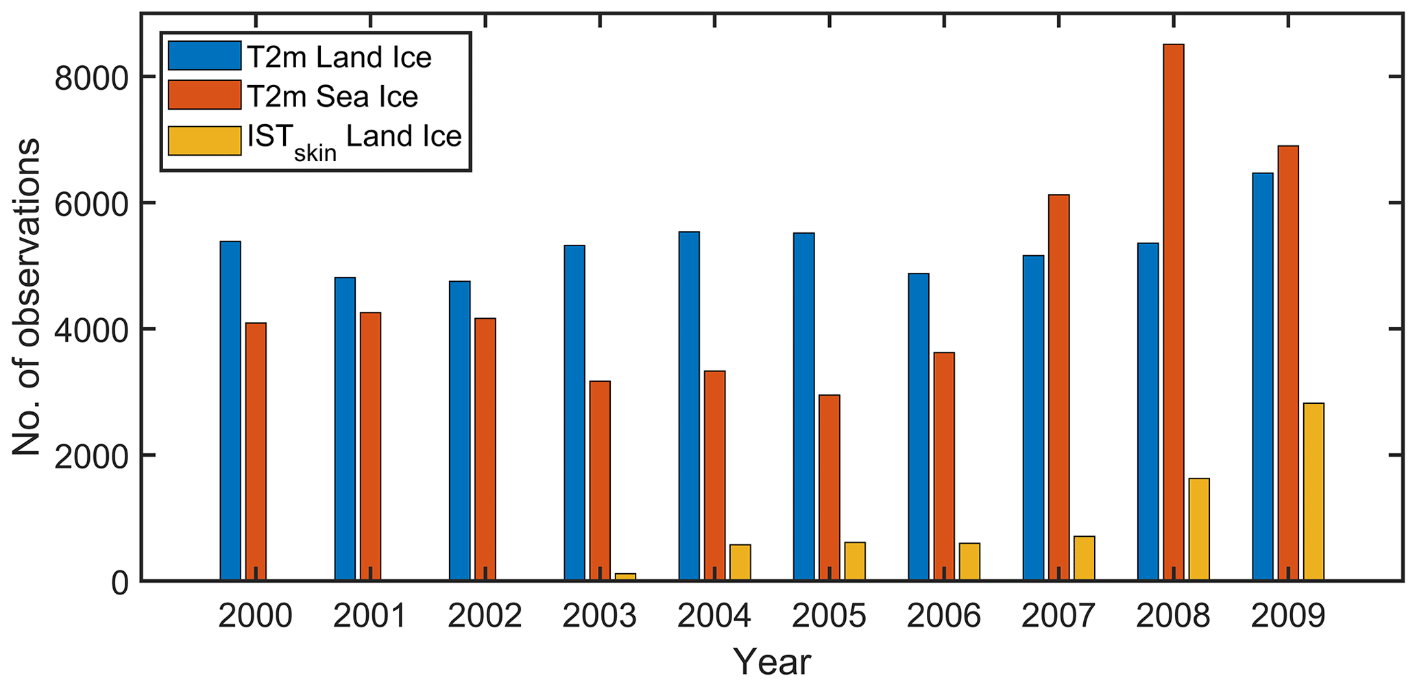
Figure 1 Total number of daily averaged in situ observations of T2m and IST_skin over Arctic land ice and sea ice per year covering the period 2000–2009.

Table 1 Overview of in situ observations used in this study, covering the period 2000–2009.

2.2 Satellite data

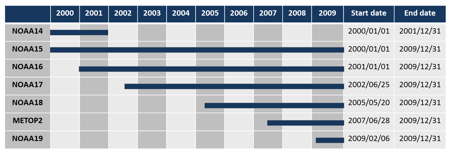
The satellite data used in this study are from the Arctic and Antarctic Ice Surface Temperatures from thermal Infrared satellite sensors (AASTI; Dybkjær et al., 2014, 2018; Høyer et al., 2019) dataset, covering high-latitude seas, sea ice, and ice sheet with clear-sky surface temperatures based on satellite infrared measurements from the CLARA-A1 dataset compiled by EUMETSAT's Climate Monitoring, Satellite Application Facility (CM-SAF; Karlsson et al., 2013). The dataset is based on one of the longest existing satellite records from the Advanced Very High Resolution Radiometer (AVHRR) instruments on board a long series of NOAA satellites. AASTI contains swath-based (i.e. Level 2; L2) ice surface skin temperature (IST_{skin_L2}) data processed and error corrected on the original Global Area Coverage (GAC) grid. The first version of the AASTI product, which is used in this study, is available from 2000 to 2009 in the original projection and resolution (L2), i.e. ∼0.05 arc degree resolution and multiple daily coverage. Since 2000, seven different AVHRR instruments have been orbiting the globe, each 14 times per day, thus providing approximately bi-hourly coverage of the polar regions (Fig. 2). The number of operational satellites increased from two to six from 2000 to 2009. The IST algorithm used to generate the AASTI dataset is based on thermal infrared brightness temperatures of AVHRR channels 4 (centre wavelength at ∼11 µm) and 5 (centre wavelength at ∼12 µm) and the satellite zenith angle. The algorithm is a split window algorithm, working within three temperature domains for each individual satellite (Key et al., 1997). The retrieval calibration of each domain has been done by relating modelled surface temperatures with modelled top-of-atmosphere brightness temperatures, determined by a radiative transfer model (Dybkjær et al., 2014). Cloud masking has been performed using the Polar Platform System (PPS) cloud processing software (Dybbroe et al., 2005a, b).

Figure 2 NOAA and Metop satellites carrying the AVHRR sensor, used for AASTI version 1.

As discussed in Merchant et al. (2017), satellite-based climate data records should include uncertainty estimates. The AASTI IST_{skin_L2} data come with uncertainties divided into three independent uncertainty components, each with different characteristics: the random uncertainty (μ_{rnd_L2}), a locally systematic uncertainty (μ_{local_L2}), and a large-scale systematic (“global”) uncertainty (μ_{glob_L2}). These three components have been chosen since they behave differently when aggregating the observations in time or space (see Sect. 3.2). This uncertainty methodology has been developed within the sea surface temperature (SST) community (Bulgin et al., 2016; Rayner et al., 2015) and will be followed here. The total uncertainty on the IST_{skin_L2}, μ_{total_L2}, is calculated by summing each component in quadrature (i.e. square root of sum of squares). Excluding the cloud mask uncertainty, grid cell systematic uncertainties (μ_{glob_L2}) are set to a fixed value of 0.1 ^∘C to represent systematic uncertainties in the forward models (see e.g. Merchant et al., 1999; Merchant and Le Borgne, 2004). The AASTI IST_{skin_L2} data also come with a quality level (QL) from 1 (bad data) to 5 (best quality), with the addition of level 0 (no data) (GHRSST Science Team, 2010).

Here, we have aggregated the AASTI IST_{skin_L2} observations into 3-hourly and daily gridded Level 3 (L3) averages of IST_{skin_L2} on a fixed 0.25^∘ by 0.25^∘ regular geographical grid. This grid was chosen within the EUSTACE project to ensure a common grid to be used globally. The daily gridded averages (IST_{skin_L3}) are calculated by averaging all available IST_{skin_L2} observations with a quality flag of 4 (good) or 5 (best) for a given date and within the 0.25^∘ bin. This has been done to facilitate the development of the relationship model and to ease the user uptake. The data in the daily aggregated files contain mean surface temperature observations from 00:00 to 24:00 LST, 3-hourly bin averages of surface temperatures, and also the number of observations in the eight time bins during each day. The 3-hourly numbers of observations are used to estimate the satellite sampling throughout the day, and the 3-hourly temperature data are used to gain confidence in the daily cycle estimates (see quality checks below). Figure 3 shows the mean number of observations per day in each of the eight time intervals given in local time for the Arctic region. The variation in coverage throughout the day is a combined effect of the satellite overpassing, performance of the cloud screening algorithm, and the cloud-free conditions during the day. In addition, the fixed 0.25^∘ regular geographical grid results in a decreasing L3 bin area when approaching the North Pole. The maximum satellite coverage is generally seen around 80^∘ N with a minimum at the North Pole. Cloud-free conditions over the GrIS are primarily observed around noon and the early afternoon.

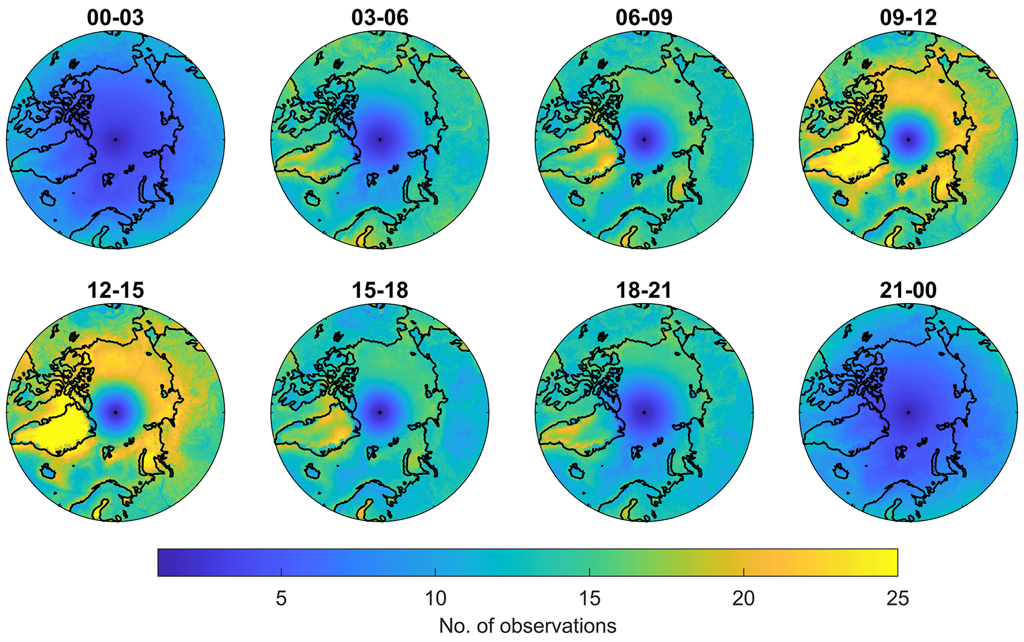
Figure 3 Mean number of observations per day in the L3 bins for each of the eight local solar time intervals, averaged for the period 2000–2009.

In order to best resolve the diurnal cycle with satellite information, we require data during both the night (between 18:00 and 06:00 LST) and the day (between 06:00 and 18:00 LST) in order to calculate IST_{skin_L3}. To identify sea ice, we use an ice mask for which sea ice is characterized by sea ice concentrations above 30 % according to the EUMETSAT OSISAF Global Sea Ice Concentration Climate Data Record (Tonboe et al., 2016). A few more checks have been set up in order to minimize the temporal sampling errors, the effects of undetected clouds and outliers, and inconsistencies between the ice mask and the surface temperatures. Following Høyer et al. (2018), the IST_{skin_L3} is discarded if one of the following criteria is met:

• IST_{skin_L3} exceeds +5 ^∘C, indicating inconsistency between the ice mask and the surface temperatures.

• The standard deviation of satellite IST_{skin_L2} during 1 d exceeds 7.07 ^∘C, corresponding to a sinusoidal daily cycle with a difference between day and night of 20 ^∘C.

• The difference between IST_{skin_L3} and the average of all available 3 h bin averages exceeds 10 ^∘C.

• IST_{skin_L3} is more than 10 ^∘C colder than the corresponding average of up to 24 neighbouring cloud-free observations (in a 5-by-5 grid cell square) with the same surface type.

The criteria above have been derived from analysis and inspection of the satellite data and with considerations to the results presented in Nielsen-Englyst et al. (2019). Inconsistencies between the ice mask and surface temperature typically occur along the coasts and sea ice edge, where the OSISAF product is subject to land-spillover effects causing spurious ice in ice-free areas (Lavergne et al., 2019). Using a surface temperature threshold of 5 ^∘C reduces the land-spillover effects and results in increased consistency between the ice mask and the surface temperatures.

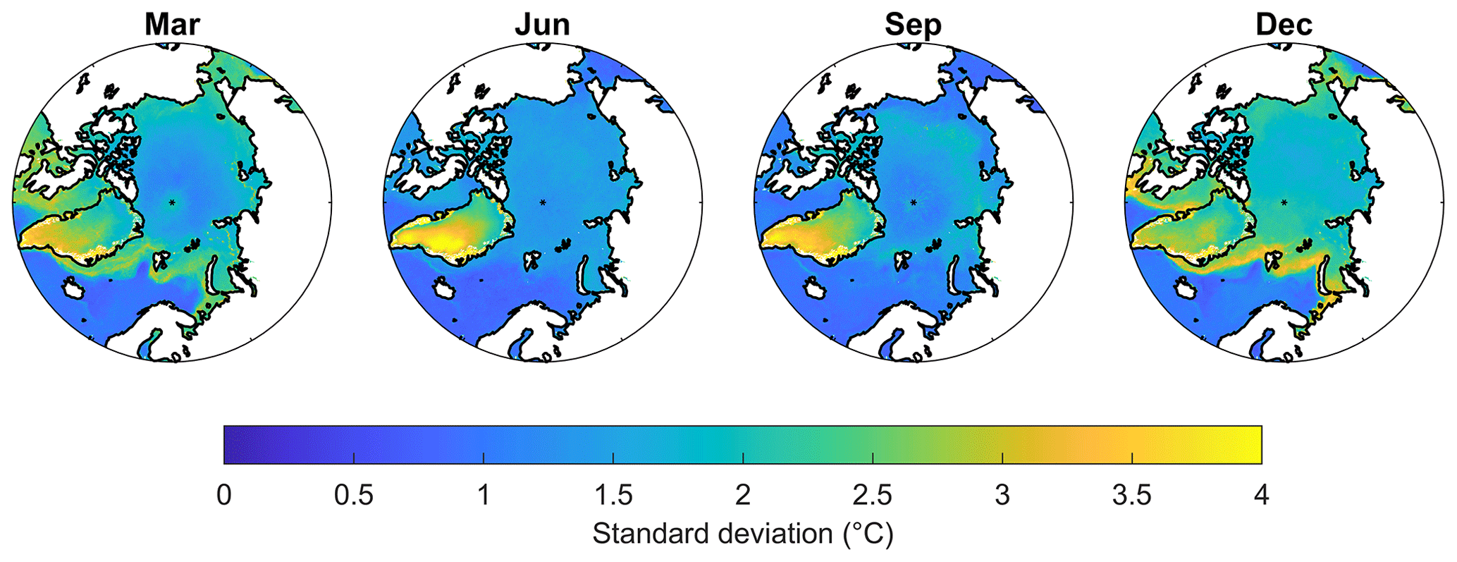
Figure 4 Standard deviations (^∘C) of daily satellite surface temperature observations for March, June, September, and December of each year averaged for the years 2000–2009.

The satellite-derived surface temperature has seasonal differences in daily variability, with the largest standard deviations during the summer in Greenland and during the winter for sea ice, when the freeze-up of sea ice causes higher variability along the sea ice margin (Fig. 4). The main uncertainty components of the IST_{skin_L3} estimates are erroneous cloud screening and the spatial variance of snow and ice surface emissivity, which are not accounted for in the retrieval algorithm. The presence of non-detected clouds will contribute to increased standard deviations and usually a cold IST_{skin_L3} bias, since the cloud tops and other atmospheric constituents are generally colder than the surface (Dybkjær et al., 2012).

2.2.1 Validation

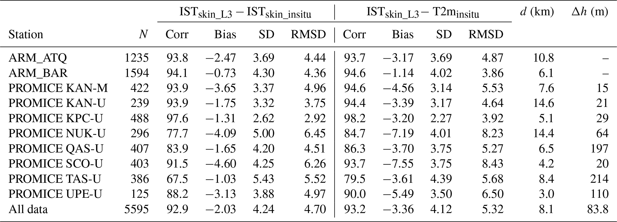
Additional satellite versus in situ differences arise when comparing satellite observations with pointwise ground measurements due to different spatial and temporal characteristics. To assess the magnitude of these effects, the IST_{skin_L3} data have been validated against in situ observations from the PROMICE and ARM stations. Table 2 shows the validation results of daily IST_{skin_L3} against in situ skin temperatures (IST_{skin_insitu}) and in situ 2 m air temperatures (T2m_insitu). The maximum matchup distance is 14.6 km, and the average distance is 8.1 km, considering the AWSs in Table 2. The topography mask included in the HIRHAM5 regional climate model (see e.g. Langen et al., 2015) has been used to calculate the differences in elevation (Δh) between the in situ stations and corresponding satellite pixels. There is no clear correlation between the large biases and large elevation differences from this table, but the elevation effects are contributing to the spatial sampling error. The spatial and temporal sampling errors contribute to the overall uncertainty, but effects from erroneous cloud screening, algorithm simplifications, and uncertainties in the in situ observations are also included in the results. Previous studies find that erroneous cloud screening (undetected clouds) is one of the main reasons for the cold biases observed when comparing satellite-observed IST with in situ measurements (Hall et al., 2004, 2012; Koenig and Hall, 2010; Østby et al., 2014; Westermann et al., 2012). Another important contribution is the effect of comparing clear-sky satellite observations with all-sky in situ observations, as discussed in Nielsen-Englyst et al. (2019). In general, IST_{skin_L3} correlates better with T2m_insitu than with the IST_{skin_insitu}. Moreover, the IST_{skin_L3}–T2m_InSitu difference shows smaller standard deviations than IST_{skin_L3}–IST_{skin_insitu}. However, as expected the biases and root-mean-squared differences (RMSDs) are larger for the IST_{skin_L3}–T2m_insitu differences than for the IST_{skin_L3}–IST_{skin_insitu} differences. The reason is that the radiometric surface skin temperature can be significantly different from the surface air temperature measurements (Adolph et al., 2018; Hall et al., 2008; Hudson and Brandt, 2005; Nielsen-Englyst et al., 2019; Vihma et al., 2008). On average, the skin temperature is colder than the air temperature (Nielsen-Englyst et al., 2019), resulting in even more negative biases, when the IST_{skin_L3} is compared to in situ measured T2m, instead of in situ skin temperatures. The generally high correlations are dominated by the synoptic (2–5 d) and seasonal variations, which are pronounced in both IST and T2m.

Table 2 Validation of daily AASTI v.1 Level 3 IST (IST_{skin_L3}) against in situ IST_skin (IST_{skin_insitu}) and T2m observations (T2m_insitu). N: number of matchups; Corr: correlation; SD: standard deviation; RMSD: root-mean-square difference. d is the matchup distance and Δh is the difference in elevation (AWS − satellite).

3 Methods

3.1 Regression model

Nielsen-Englyst et al. (2019) analysed a large number of in situ stations with simultaneous T2m and IST_skin observations and showed that empirical relationships exist between T2m and IST_skin. However, it was also shown that the relationships varied for different regions. Based upon these results, it was decided to use a simple-regression-based method in this paper to derive the daily mean T2m from the satellite IST_{skin_L3} observations. Separate regression models have been derived for land ice and sea ice. To test different types of regression models, the IST_{skin_L3} data have been matched up with in situ observations for each day (Høyer et al., 2018). This is done by requiring a distance to the nearest in situ site of less than 15 km. The average matchup distance is 8.6 and 7.2 km for land ice and sea ice, respectively, which means that all in situ observations are made within the area of the satellite pixel. The corresponding mean elevation difference is 30 m (while the absolute mean elevation difference is 45 m) and is calculated using the topography mask included in HIRHAM5 (Langen et al., 2015) for the 23 GrIS AWSs. Out of the 23 AWSs, four of them (GC-net JAR1, TAS_U, QAS_U, and UPE_U) have corresponding elevation differences above 100 m. In Sect. 4.3, the effect of these AWSs has been estimated and discussed. All in situ observations, described in Sect. 2.1., have been matched with IST_{skin_L3} data, resulting in a total number of daily matchups of 65 810 from 275 different observation sites (see Table 1). These have been divided into two subsets: one for training and one for validation of the different regression models for land ice and sea ice, respectively. This has been done while ensuring similar coverage of training and validation data over the two domains, which is shown in Fig. 5. The result is that 40 % (13 792 matchups) are used for testing the regression models (and generating the regression coefficients), and the remaining 60 % (20 872 matchups) are left for validation of the regression models over land ice. Over sea ice 48 % (15 035 matchups) are used for testing, and 52 % (16 111 matchups) are left for validation.

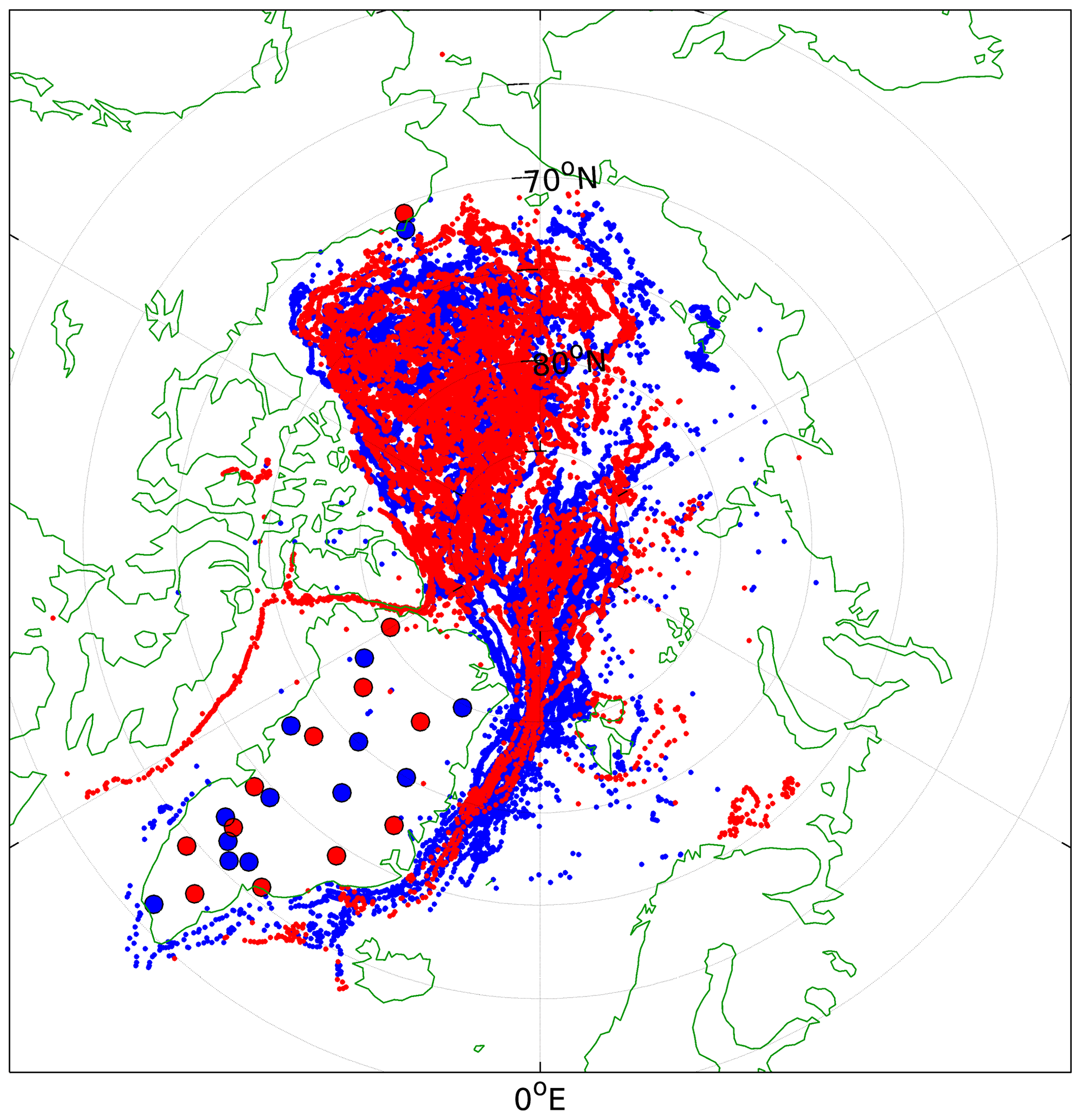
Figure 5 Positions of matchups on sea ice and land ice (red: training; blue: validation).

The regression model is based on multiple linear regression analysis using least squares (Menke, 1989). The multiple linear regression analysis equations can be written in matrix form,

$$\begin{array}{}\text{(1)}& {\displaystyle }& {\displaystyle }{\mathit{d}}^{\text{obs}}=\mathbf{G}\mathit{m}+\mathit{e},\text{(2)}& {\displaystyle }& {\displaystyle }{\mathit{d}}^{\text{pre}}=\mathbf{G}\mathit{m},\end{array}$$

where d^obs and d^pre are vectors containing the observed and modelled in situ air temperatures, respectively, G is a matrix containing the various predictors, m is a vector containing regression coefficients, and e is the fitting error.

The regression coefficients are found using damped least squares (Menke, 1989). The least-squares method is used since the problem is generally over-determined, and the damping is added to limit effects of noisy data. The regression coefficients are thus given as

$$\begin{array}{}\text{(3)}& {\displaystyle }& {\displaystyle }{\mathbf{G}}^{-\mathrm{g}}={\left({\mathbf{G}}^T\mathbf{G}+{\mathit{\epsilon }}^{\mathrm{2}}\mathbf{I}\right)}^{-\mathrm{1}}{\mathbf{G}}^T,\text{(4)}& {\displaystyle }& {\displaystyle }\mathit{m}={\mathbf{G}}^{-\mathrm{g}}{\mathit{d}}^{\text{obs}},\end{array}$$

where G^−g is called the generalized inverse, ε is a damping factor, and I is an identity matrix (with ones in the diagonal and zeros elsewhere). The superscript operator T denotes transposing and −1 denotes inversion. We have tested a range of damping factors to assess the relation to the error coefficients. A damping factor of 0.2 was chosen to avoid overfitting noise in the data, while keeping the error coefficients low.

The choice of predictors is based on current knowledge of the parameters that influence the relationship between IST_skin and T2m_insitu (Adolph et al., 2018; Hall et al., 2008; Hudson and Brandt, 2005; Nielsen-Englyst et al., 2019; Vihma and Pirazzini, 2005), limited by the available satellite data. Nielsen-Englyst et al. (2019) showed that the T2m–Tskin difference varies over the season with the smallest differences during the spring, autumn, and summer in non-melting conditions. For that reason, we have also tested the effect of including a seasonal cycle as predictor. A total of five regression models with different predictors have been tested (Høyer et al., 2018).

$$\begin{array}{llll}\text{(5)}& {\displaystyle }& {\displaystyle }{\text{ÎST}}_{\text{skin}}:& {\displaystyle }\mathrm{T}\mathrm{2}{\mathrm{m}}_{\mathrm{sat}}& {\displaystyle }={\mathit{\alpha }}_{\mathrm{0}}+{\mathit{\alpha }}_{\mathrm{1}}{\text{IST}}_{\text{skin\_L3}}{\displaystyle }& {\displaystyle }{\text{ÎST}}_{\text{skin}}\text{SWd}:& {\displaystyle }\mathrm{T}\mathrm{2}{\mathrm{m}}_{\mathrm{sat}}& {\displaystyle }={\mathit{\alpha }}_{\mathrm{0}}+{\mathit{\alpha }}_{\mathrm{1}}{\text{IST}}_{\text{skin\_L3}}\\ \text{(6)}& {\displaystyle }& {\displaystyle }& {\displaystyle }& {\displaystyle }+{\mathit{\alpha }}_{\mathrm{2}}\text{SWd}{\displaystyle }& {\displaystyle }{\text{ÎST}}_{\text{skin}}\text{WS}:& {\displaystyle }\mathrm{T}\mathrm{2}{\mathrm{m}}_{\mathrm{sat}}& {\displaystyle }={\mathit{\alpha }}_{\mathrm{0}}+{\mathit{\alpha }}_{\mathrm{1}}{\text{IST}}_{\text{skin\_L3}}\\ \text{(7)}& {\displaystyle }& {\displaystyle }& {\displaystyle }& {\displaystyle }+{\mathit{\alpha }}_{\mathrm{2}}\text{WS}{\displaystyle }& {\displaystyle }{\text{ÎST}}_{\text{skin}}\text{Lat}:& {\displaystyle }\mathrm{T}\mathrm{2}{\mathrm{m}}_{\mathrm{sat}}& {\displaystyle }={\mathit{\alpha }}_{\mathrm{0}}+{\mathit{\alpha }}_{\mathrm{1}}{\text{IST}}_{\text{skin\_L3}}\\ \text{(8)}& {\displaystyle }& {\displaystyle }& {\displaystyle }& {\displaystyle }+{\mathit{\alpha }}_{\mathrm{2}}\text{Lat}{\displaystyle }& {\displaystyle }{\text{ÎST}}_{\text{skin}}\text{Season}:& {\displaystyle }\mathrm{T}\mathrm{2}{\mathrm{m}}_{\mathrm{sat}}& {\displaystyle }={\mathit{\alpha }}_{\mathrm{0}}+{\mathit{\alpha }}_{\mathrm{1}}{\text{IST}}_{\text{skin\_L3}}\\ {\displaystyle }& {\displaystyle }& {\displaystyle }& {\displaystyle }+{\mathit{\alpha }}_{\mathrm{2}}\cos \left((t\cdot \mathrm{2}\mathit{\pi })/\left(\mathrm{1}\mathrm{yr}\right)\right)\\ \text{(9)}& {\displaystyle }& {\displaystyle }& {\displaystyle }& {\displaystyle }+{\mathit{\alpha }}_{\mathrm{3}}\sin \left((t\cdot \mathrm{2}\mathit{\pi })/\left(\mathrm{1}\mathrm{yr}\right)\right)\end{array}$$

The regression model in Eq. (8) is limited to an offset and a scaling of IST_{skin_L3}, where the latter term accounts for the synoptic and seasonal variations, which are the dominating factors in both the IST and T2m variability. This part is thus included in all regression models tested. The other regression models also have a third predictor, which is included to examine how to best represent the residual variations in the T2m–IST difference. The model in Eq. (9) uses theoretical top-of-atmosphere shortwave radiation, Eq. (10) uses the wind forcing (from ERA-I and ERA5, respectively), Eq. (11) uses latitude variation, and Eq. (12) uses a seasonal variation. In the regression model in Eq. (12), the seasonal variation is assumed to be the shape of a cosine function, $A\cdot \cos \left(\right(t\cdot \mathrm{2}\mathit{\pi })/(\mathrm{1}\mathrm{yr})-\mathit{\phi })$, where A is the amplitude, φ is the phase and t is time. Since $\cos (x_{\mathrm{1}}-x_{\mathrm{2}})=\cos \left(x_{\mathrm{1}}\right)\cos \left(x_{\mathrm{2}}\right)+\sin \left(x_{\mathrm{1}}\right)\sin \left(x_{\mathrm{2}}\right)$, the seasonal cycle can be rewritten to the form in Eq. (12) with $A=\sqrt{{\mathit{\alpha }}_{\mathrm{2}}^{\mathrm{2}}+{\mathit{\alpha }}_{\mathrm{3}}^{\mathrm{2}}}$ and $\mathit{\phi }=\arctan ({\mathit{\alpha }}_{\mathrm{3}}/{\mathit{\alpha }}_{\mathrm{2}})$.

Table 3 Statistics on the relation between observed and modelled temperatures for the training data. N: number of matchups used for testing; Corr: correlation; RMSD: root-mean-square difference. Since, the training data are used for the regression, the bias is zero, and thus the standard deviation equals RMSD.

Table 4 Model regression coefficients for ÎST_skinSeason.

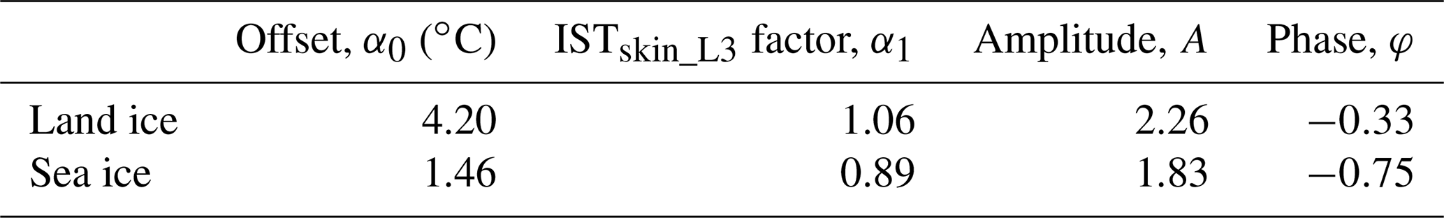
The training data have been used to calculate the regression coefficients for each regression model covering the land ice and sea ice. The performance of each regression model has been investigated using the training data, and the results are shown in Table 3. The best performance is found by using the regression model where T2m_sat is predicted from IST_{skin_L3} combined with a seasonal variation (ÎST_skinSeason). This model predicts T2m_sat better compared to the other regression models, with correlations above 96 % and RMSD values of 3.25–3.28 ^∘C against training data for both surface types (Table 3). In the following, we will use the regression model given in Eq. (12) with the seasonal term included and with separate regression coefficients for land ice and sea ice (see Table 4). The phase corresponds to a maximum on the 19 January and 12 February for land ice and sea ice, respectively. This is in agreement with Nielsen-Englyst et al. (2019), who found the strongest clear-sky inversion during the winter months (December–February) for all sites included in the analysis except from the ones located in the lower ablation zone (not included here), where pronounced surface melt takes place for long periods of time.

3.2 Uncertainty estimates for T2m_sat

Uncertainty estimates on the derived T2m_sat are crucial to facilitate the usage of the dataset in modelling and for monitoring purposes. The uncertainty estimates of the satellite-derived T2m_sat data follow the approach in Bulgin et al. (2016) and Rayner et al. (2015), which has also been used for the AASTI data. The uncertainty on a single T2m_sat estimate is divided into random, locally correlated, and systematic uncertainty components, with the total uncertainty μ_{total_T2m} given as the square root of the sum of the three squared components:

$${\mathit{\mu }}_{\text{total}\mathit{\_}\text{T2m}}=\sqrt{{\mathit{\mu }}_{\text{rnd}\mathit{\_}\text{T2m}}^{\mathrm{2}}+{\mathit{\mu }}_{\text{local}\mathit{\_}\text{T2m}}^{\mathrm{2}}+{\mathit{\mu }}_{\text{glob}\mathit{\_}\text{T2m}}^{\mathrm{2}}}.$$

The random uncertainty component for the T2m_sat belonging to a particular grid cell at a particular point in time is found by propagating the AASTI IST_{skin_L3} random uncertainty through the regression model:

$${\mathit{\mu }}_{\text{rnd}\mathit{\_}\text{T2m}}=\sqrt{{\left({\mathit{\alpha }}_{\mathrm{1}}{\mathit{\mu }}_{\text{rnd\_L3}}\right)}^{\mathrm{2}}},$$

with μ_{rnd_L3} given as the aggregated μ_{rnd_L2}:

$${\mathit{\mu }}_{\text{rnd\_L3}}={\displaystyle \frac{{\mathit{\mu }}_{\text{rnd\_L2}}}{\sqrt{N}}},$$

where N is the number of observations for each bin in the aggregation from L2 to L3. The $\sqrt{N}$ reduction applies because the random uncertainty of each L2 data point that goes into the L3 calculation is by definition independent from the other.

The L3 global uncertainty component does not average out in any aggregation and is thus transferred directly from the L2 uncertainty estimate and multiplied by α₁ to make up μ_{glob_T2m}:

$${\mathit{\mu }}_{\text{glob}\mathit{\_}\text{T2m}}={\mathit{\alpha }}_{\mathrm{1}}{\mathit{\mu }}_{\text{glob\_L3}}={\mathit{\alpha }}_{\mathrm{1}}\cdot \mathrm{0.1}{}^{\circ }\mathrm{C}.$$

The μ_{local_T2m} contains the local uncertainty component of L2, a sampling error μ_{lsamp_L3} related to sampling errors in space and time due to the aggregation, a relationship error, cloud mask uncertainty, etc. When aggregating from L2 to daily L3, additional sources of uncertainty enter through the gridding process as IST_{skin_L3} can only be retrieved for clear-sky pixels. This introduces a temporal and spatial sampling uncertainty. If all our satellite observations were obtained during all-sky conditions, we assume that the high polar temporal coverage is such that the temporal sampling uncertainty in the L3 files can be set to zero. However, this is not the case, and using only clear-sky observations generally leads to a clear-sky bias in averaged IST_skin satellite observations when compared to in situ observations (Hall et al., 2012; Nielsen-Englyst et al., 2019; Rasmussen et al., 2018). The relationship error represents the standard deviation of the residuals calculated at in situ stations, where both skin and air temperatures are available, i.e. T2m_sat–T2m_insitu. Estimating all the different components that make up the μ_{local_T2m} is a very challenging task and is out of the scope of this paper. Instead, we estimate the μ_{local_T2m} component using a simple regression model fitted to the satellite-derived T2m and in situ T2m differences. Separate models have been chosen for the land ice and sea ice, due to the differences in the error characteristics. The variables to include in the uncertainty regression models have been chosen from a careful examination of the matchup dataset. For land ice and sea ice the most relevant variables were the IST_{skin_L3} itself and the number of 3 h time bins with observations in the L3, N_bins.

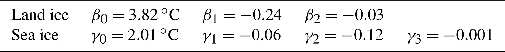
For land ice the regression model for μ_{local_T2m} is given as follows:

$$\begin{array}{}\text{(10)}& {\mathit{\mu }}_{\text{local}\mathit{\_}\text{T2m}\mathit{\_}\text{landice}}={\mathit{\beta }}_{\mathrm{0}}+{\mathit{\beta }}_{\mathrm{1}}{\text{IST}}_{\text{skin\_L3}}+{\mathit{\beta }}_{\mathrm{2}}{N}_{\text{bins}},\end{array}$$

while the regression model for sea ice is given as

$$\begin{array}{ll}{\displaystyle }{\mathit{\mu }}_{\text{local}\mathit{\_}\text{T2m}\mathit{\_}\text{seaice}}=& {\displaystyle }{\mathit{\gamma }}_{\mathrm{0}}+{\mathit{\gamma }}_{\mathrm{1}}{\text{IST}}_{\text{skin\_L3}}+{\mathit{\gamma }}_{\mathrm{2}}{\text{IST}}_{{\text{skin}}_{\text{L3}}}^{\mathrm{2}}\\ \text{(11)}& {\displaystyle }& {\displaystyle }+{\mathit{\gamma }}_{\mathrm{3}}{N}_{\text{bins}}.\end{array}$$

The coefficients have been determined by fitting to the T2m_sat–T2m_insitu standard deviations calculated for the training data with IST_{skin_L3} bin intervals of 2 ^∘C and a N_bins interval of 1. The μ_{rnd_T2m} and μ_{glob_T2m} components have been removed from the standard deviations in each bin as well as an assumed in situ uncertainty of 0.1 ^∘C and an average sampling uncertainty of 0.5 ^∘C (Høyer et al., 2017a; Reeves Eyre and Zeng, 2017) before fitting the regression models. The optimal regression coefficients for each domain are listed in Table 5.

Table 5 Uncertainty model regression coefficients.

4 Results

In Sect. 3.1, we selected the best (Eq. 12) of the five different algorithms and used it together with the derived coefficients (Tables 3 and 4) to retrieve T2m from satellite surface temperature estimates. The derived dataset consists of daily estimates of near-surface air temperature on a 0.25^∘ regular latitude–longitude grid, during the period 2000–2009 (Høyer et al., 2018; Kennedy et al., 2019). Days with clouds and few clear-sky observations (as explained in Sect. 2.2) are not included in the dataset. However, for those days when the satellite-derived T2m product is available, it provides an estimate of the daily averaged all-sky T2m (see Sect. 5). Each temperature estimate is associated with three components of uncertainty on the 0.25^∘ daily scale: a random uncertainty, a synoptic-scale correlated uncertainty, and a globally correlated uncertainty excluding uncertainties related to the masking of clouds. The three types of uncertainties are also gathered in a total uncertainty estimate (see Sect. 3.2). The land ice temperatures have been calculated for grid cells categorized as ice sheet by the ETOPO1 global relief model (Amante and Eakins, 2009), averaged to the 0.25^∘ grid. Sea ice temperatures have been calculated for grid cells with sea ice concentrations above 30 %, according to OSISAF (Tonboe et al., 2016).

4.1 Validation of T2m_sat

The derived T2m_sat product has been validated against independent in situ data (i.e. the validation subset described in Sect. 3.1). Figure 6 shows an example of the daily near-surface air temperature coverage (from 1 January 2008). Circles are in situ T2m measurements from coincidence-independent AWSs and buoys, and there seems to be quite good agreement between these and T2m_sat during this specific day. The overall model performance, when compared to all independent AWS and buoy observations, is summarized in Table 6. The satellite-derived air temperatures are about 0.3 ^∘C warmer than measured in situ air temperature for both land ice and sea ice. For the GrIS, the bias is partly explained by topographic effects (see Sect. 4.3). The correlations are above 95 % for both surface types, and the RMSD is 3.47 and 3.20 ^∘C for land and sea ice, respectively. Note that the uncertainty of the in situ data is also included in these RMSD values.

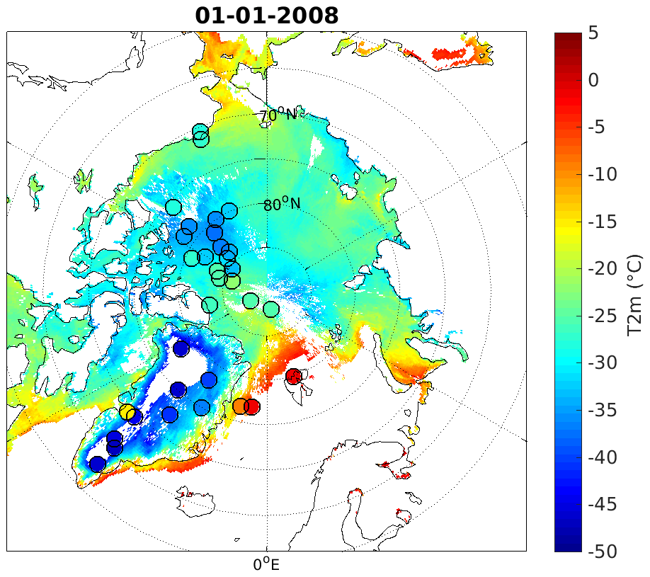
Figure 6 Daily mean 2 m air temperature over land ice and sea ice from 1 January 2008. Circles show in situ measurements.

Table 6 Statistics on the relation between satellite-derived and in situ measured temperatures for comparison with independent validation data. N: number of matchups used for validation; Corr: correlation; bias: T2m_sat–T2m_insitu difference; SD: standard deviation; RMSD: root-mean-square difference.

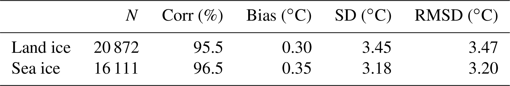
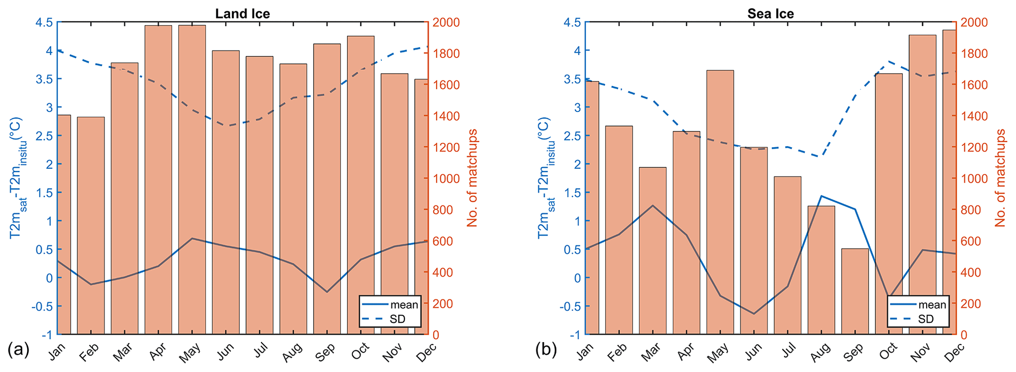
Figure 7 Estimated T2m minus observed T2m averaged for each month for (a) land ice and (b) sea ice. The dashed lines are standard deviations while the solid lines are biases. The bars show the average number of matchups for each month.

Figure 7 shows the average seasonal variation in bias and standard deviation for land ice and sea ice, respectively. For both land ice and sea ice, there is a seasonal dependency in standard deviation, with the largest values during the winter and smallest values during the summer. This is likely explained by a better cloud screening performance during sunlit periods (Karlsson and Dybbroe, 2010) and by the smaller natural thermal variability that is observed during summer conditions. Similar seasonality in performance is seen in five reanalysis products (including ERA-I/ERA5) for the GrIS (Zhang et al., 2021). As shown in Fig. 7, the average seasonal variation in bias is largest over sea ice, with the largest values in March and August. However, this seasonal tendency in bias over sea ice is only reflected at the beginning of the time period (i.e. 2000–2004). This can be seen in Fig. 8, which shows the seasonal averaged independent validation statistics for the entire period for land ice and sea ice. The figure also shows a quite stable performance over the time period for both land ice and sea ice.

Figure 8 Estimated T2m minus observed T2m (bin size of 1 ^∘C) for the full time period (bin size of 90 d) for (a) land ice and (b) sea ice. The dashed lines are standard deviations while the solid lines are bias in the upper figures. The surface plots in the middle figures show the number of matchups in each bin, while the bottom plots show the number of matchups (blue) and the cumulative percentage of matchups (red) in each time bin.

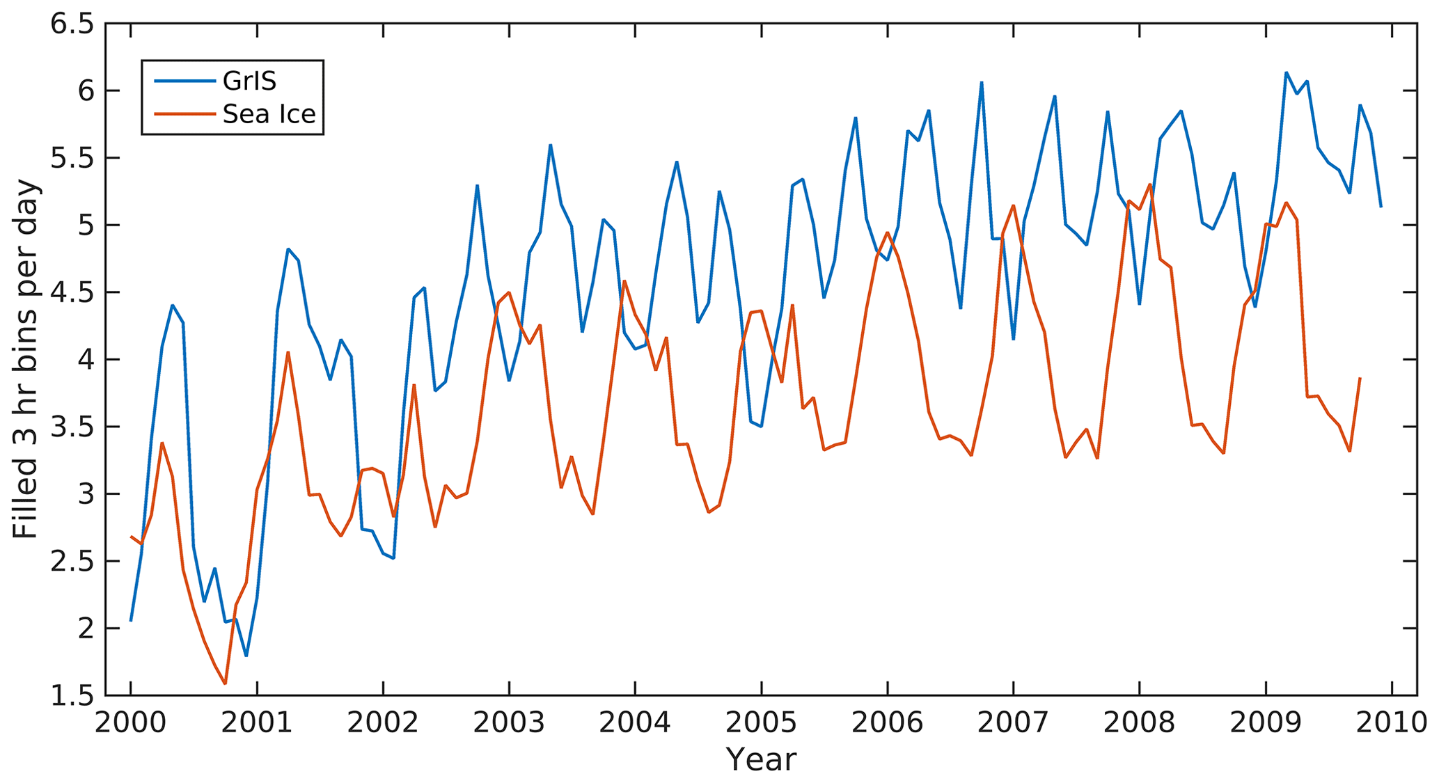
Figure 9 Average number of filled 3 h bins per day for the Greenland Ice Sheet and the Arctic sea ice.

As more satellite observations have become available over the time period, increased coverage of the surface temperature is expected over time. Figure 9 shows the average number of filled 3 h bins per day for the GrIS and Arctic sea ice for 2000–2009. Both surface types show an increase in filled 3 h bins over time, with large seasonal variations. In most years, sea ice has 1–1.5 filled bins per day more during winter than summer, due to a more extensive cloud cover over sea ice during summer (Curry et al., 1996; Beesley and Moritz, 1999). The GrIS typically has fewer filled bins per day during the winter and summer than spring and autumn, which is also explained by differences in cloud coverage (Griggs and Bamber, 2008). Note that the increase in the average number of filled 3 h bins from 2000 to 2009 is not reflected in the performance of the T2m product (Fig. 8).

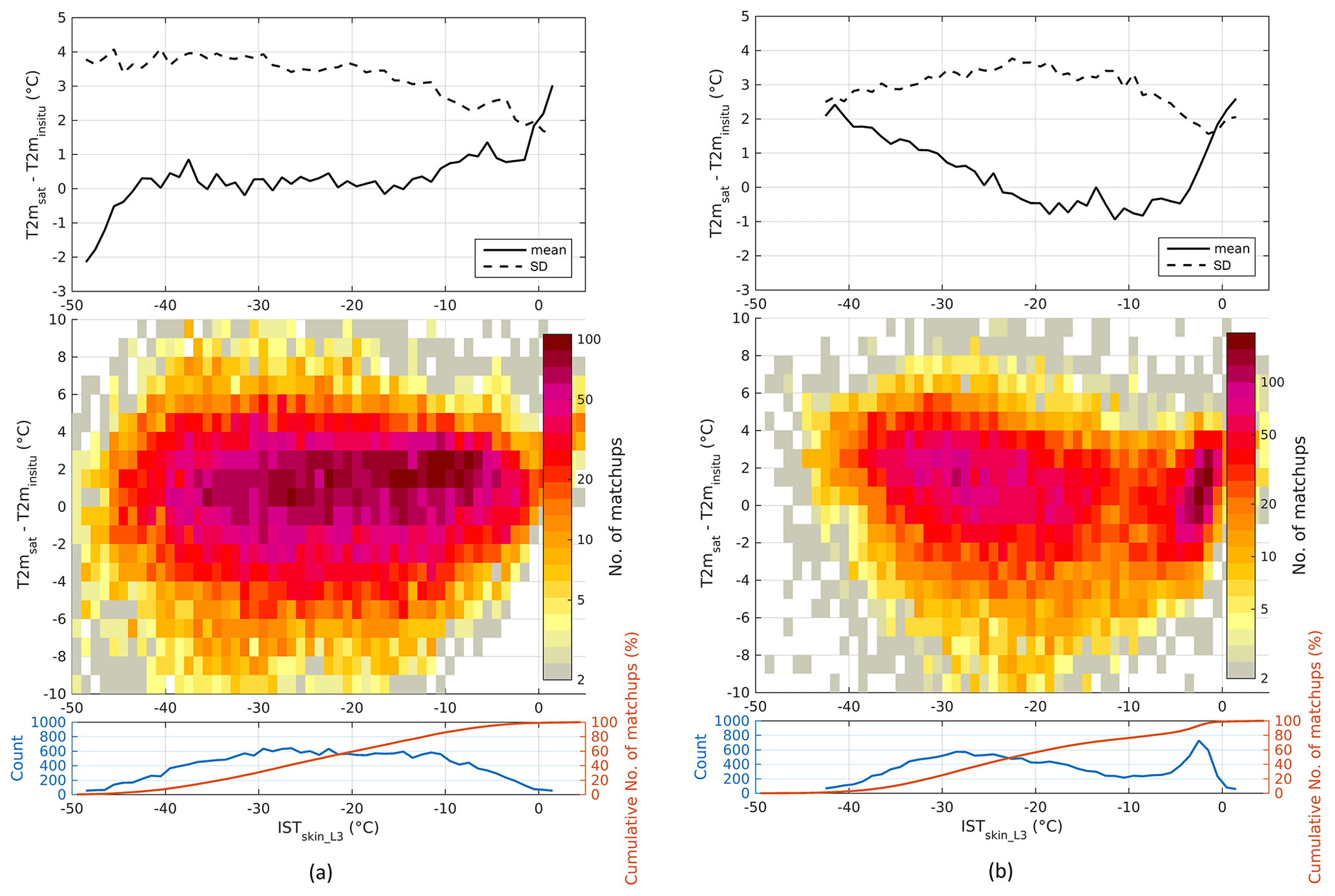
Figure 10 Estimated T2m minus observed T2m (bin size of 1 ^∘C) as a function of binned (bin size of 1 ^∘C) satellite IST_{skin_L3} for (a) land ice and (b) sea ice. The dashed lines are standard deviations while the solid lines are bias in the upper figure. The surface plots in the middle figures show the number of matchups in each bin while the bottom plots show the number of matchups (blue) and the cumulative percentage of matchups (red) in each IST_{skin_L3} bin.

Figure 10 shows T2m_sat–T2m_insitu differences plotted as a function of AASTI L3 skin temperature for land ice and sea ice. Over land ice, the standard deviation decreases as a function of IST_{skin_L3}, while the bias is around zero for IST_{skin_L3} between −45 and −10 ^∘C, positive for higher temperatures and negative for lower temperatures. For sea ice, the maximum standard deviation is found at skin temperatures of about −20 ^∘C, with smaller standard deviations for higher and lower IST_{skin_L3}. Positive biases are found for very cold skin temperatures ($<-\mathrm{25}$ ^∘C) and for temperatures around the melting point ($>-\mathrm{4}$ ^∘C), while the intermediate temperatures have a slightly negative bias. This effect is included in the uncertainty estimates as presented in Sect. 3.2, which include IST_{skin_L3} as a predictor for both land ice and sea ice.

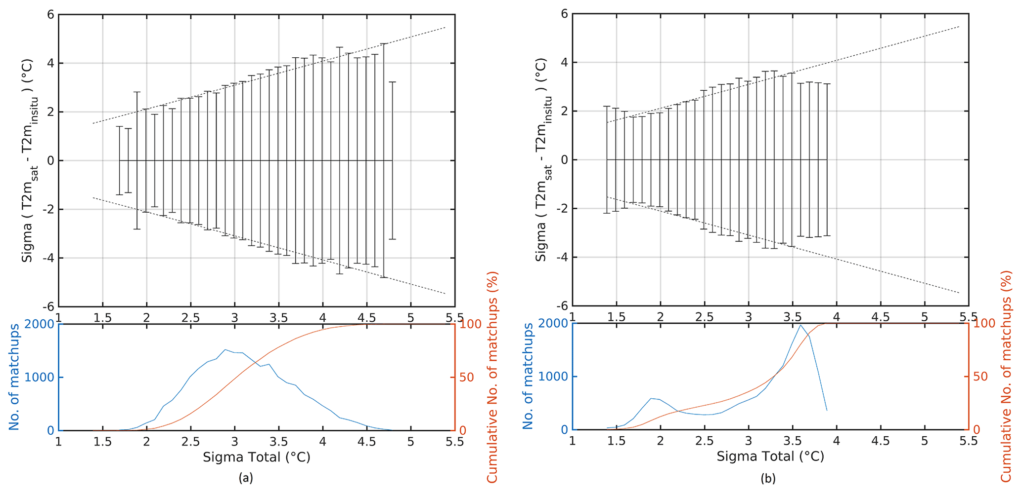
Figure 11 Satellite-estimated T2m uncertainty validation with respect to independent in situ T2m for (a) land ice and (b) sea ice. Dashed lines show the modelled uncertainty accounting for uncertainties in the in situ T2m and the sampling error. Solid black lines show 1 standard deviation of the estimated minus in situ differences for each 0.1 ^∘C bin. The bottom plots show the number of matchups (blue) and the cumulative percentage of matchups for each bin (red).

Figure 11 shows the validation results of the estimated uncertainties, where the T2m_sat–T2m_insitu difference is plotted against the theoretical total uncertainties as obtained in Sect. 3.2 for land ice and sea ice. The dashed lines represent the ideal uncertainty with the assumptions that the in situ observations have an uncertainty of 0.1 ^∘C and that the sampling uncertainty is 0.5 ^∘C. The estimated uncertainties show good agreement with the observed uncertainties when the error bars follow the dashed line, which is the case here for both land ice and sea ice.

4.2 Comparison with reanalyses

The performance of T2m_sat has been compared to the performance of T2m from ECMWF's reanalysis ERA-I (T2m_ERA-I; Dee et al., 2011) and the replacement reanalysis ERA5 (T2m_ERA5; Hersbach et al., 2020). Table 7 shows the performance of T2m_ERA-I and T2m_ERA5 against the independent in situ T2m observations, which should be compared with the performance of the regression-derived T2m_sat as shown in Table 6. The comparison may not be truly independent as a number of stations and buoys have been assimilated into the ERA-I and ERA5 data products (Dee et al., 2011; Hersbach et al., 2020), which would favour the reanalysis products in the comparison. Yet, the bias is significantly lower for T2m_sat than for both T2m_ERA-I and T2m_ERA-5, while the other validation parameters are similar, with slightly better correlation and standard deviation but slightly worse RMSD results for T2m_ERA. Previous studies have also found that ERA-I suffers from a consistent warm bias in the Arctic (Lüpkes et al., 2010; Jakobson et al., 2012; Vihma et al., 2002; Batrak and Müller, 2019; Simmons and Poli, 2014), and recent studies suggest that the warm bias still exists in ERA5 over sea ice (Wang et al., 2019; Graham et al., 2019). Similarly, recent studies found no significant improvements in 2 m temperatures over the GrIS for ERA5 compared to ERA-I (Delhasse et al., 2020; Zhang et al., 2021). Note, however, that the NCEP-CFSR, which is based on a coupled atmosphere–sea ice–ocean model, has shown better performance than ERA-I for near-surface atmospheric variables over sea ice (Jakobson et al., 2012).

Table 7 Statistics on the relation between ERA-I/ERA5 and in situ measured temperatures for independent test data. N: number of matchups used for validation; Corr: correlation; bias: T2m_ERA–T2m_insitu difference; SD: standard deviation; RMSD: root-mean-square difference.

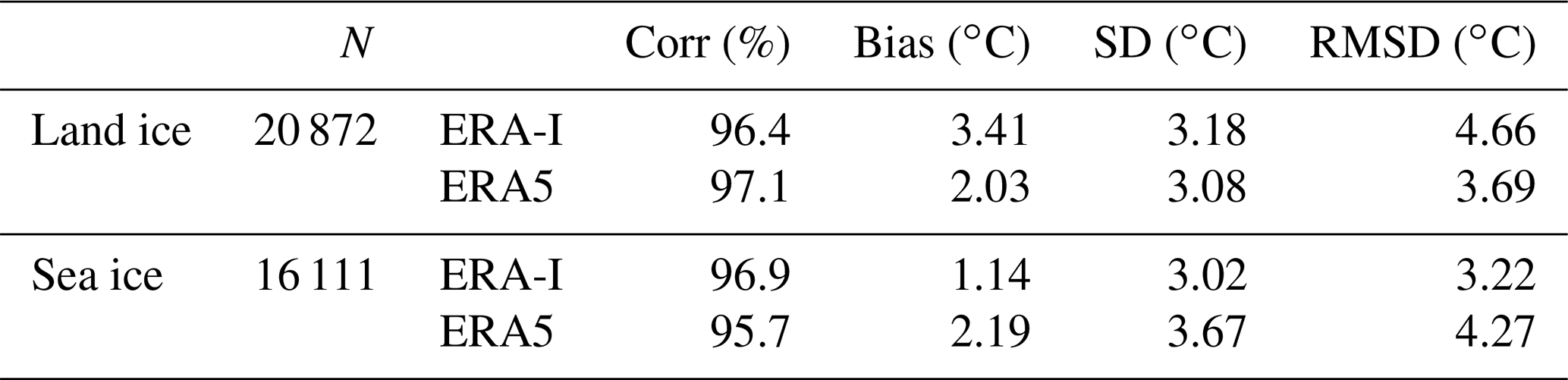
Figure 12 Root-mean-square differences (RMSDs) calculated for the (a) land ice sites and (b) sea ice sites using T2m from ERA-Interim, ERA5, and the regression model, respectively. Only buoys with more than 200 observations are included. The last two bars listed as “total” are the RMSD obtained by using all validation data.

Figure 12 shows the RMSD between in situ measured T2m and T2m_ERA-I as well as T2m_ERA5 and T2m_sat for the individual validation sites and both surface types. Due to the large number of buoys, these have been validated for each data source with all observations weighted equally. The last bars refer to the RMSD obtained by validating all validation sites in one long time series weighting all daily observations equally. The total T2m_sat agrees better with in situ observations for both surface types compared to both ERA-I and ERA5. For most land ice stations, the T2m_sat outperforms ERA-I and ERA5. One exception is the ARM station (BAR), where a bias of 2.49 ^∘C gives rise to a relatively large RMSD for T2m_sat. This is likely explained by physical differences between the seasonal snow-covered sites and the GrIS sites, which are not fully captured by the regression model. ERA5 is significantly better than ERA-I over the GrIS, but ERA5 performs worse than both ERA-I and T2m_sat over sea ice. Over sea ice, T2m_ERA-I agrees better with in situ observations from the ECMWF data stream and Polarstern. However, these may be assimilated into both ERA-I and ERA5. The validation against Polarstern is relatively good even though the temperature measurements are made at 29 m height. This is likely because the data are mainly from the summer, when the vertical temperature gradients in the boundary layer are mostly small, and the performance of the cloud screening algorithm reaches its maximum. The independent in situ observations by ACSYS, CRREL, DAMOCLES, and FRAMZY are better reproduced by the satellite-derived T2m. The errors in the T2m_ERA-I/T2m_ERA5 and T2m_sat datasets are expected to be independent and uncorrelated. For that reason, a combination of either T2m_ERA-I or T2m_ERA5 and T2m_sat can lead to an improved T2m estimate.

4.3 Topographic effects

The effects from topography over the GrIS have been assessed by introducing a new matchup dataset that ensures that the elevation difference between satellite and in situ observations is less than 100 m over the GrIS. Excluding those AWSs (4 out of 23) with a larger elevation difference than 100 m results in a reduction of the training dataset of 2935 matchups (i.e. from GC-net_JAR1 and PROMICE TAS_U) and a reduction in the validation dataset of 560 matchups (i.e. from PROMICE QAS_U and UPE_U). The performance of the satellite-derived T2m improves the bias in particular, which decreases to 0.07 ^∘C, while the standard deviation decreases to 3.41 ^∘C over land ice. ERA-I and ERA5 show limited changes in performance, with slightly increased biases of 3.48 and 2.07 ^∘C and standard deviations of 3.14 and 3.08 ^∘C, respectively, when introducing the new matchup dataset over land ice. A similar good performance of the regression model is found when the two AWSs in the validation subset are kept. Despite the increased performance of the regression model, we have included all observations in the training of the model to ensure a robust and spatial representative solution.

4.4 Analysis of T2m_sat

The monthly mean T2m_sat is shown in Fig. 13 for March, June, September and December averaged over the period 2000–2009. The interior and northern part of the GrIS is typically colder than other parts of the Arctic in all months, while the warmest regions are found along the sea ice marginal ice zone and the ablation zone of the GrIS. Limited spatial variability is seen over the Arctic sea ice during summer.

Figure 13 Monthly mean T2m_sat during March, June, September, and December, averaged for the period 2000–2009.

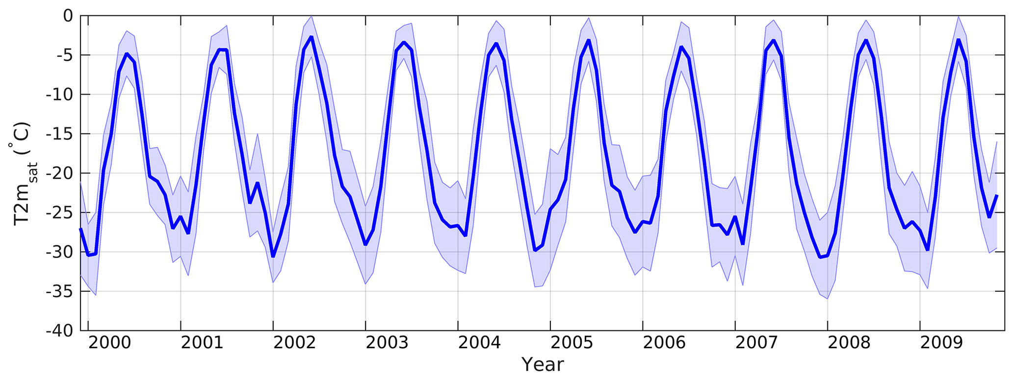
Figure 14 Monthly mean T2m_sat for the Greenland Ice Sheet. The shading represents the variability.

Figure 14 shows the monthly mean near-surface air temperature estimates averaged over the GrIS for the period 2000–2009. The GrIS records a distinct annual cycle in near-surface air temperature, with the maximum temperatures of around −4 ^∘C during July and minimum temperatures of about −28 ^∘C during winter. The range in monthly mean air temperature is in agreement with those reported by van As et al. (2011) at a number of PROMICE AWSs. The temporal variability is largest during winter due to a larger cloud radiative effect (compared to near-zero during summer) and a larger meridional temperature gradient resulting in a more vigorous atmospheric circulation in winter (Serreze et al., 1993). In addition, the temporal variability is lower during summer due to the fact that when the surface begins to melt, the sensible heat is used for melting and hence reducing surface air temperature variability (Steffen, 1995).

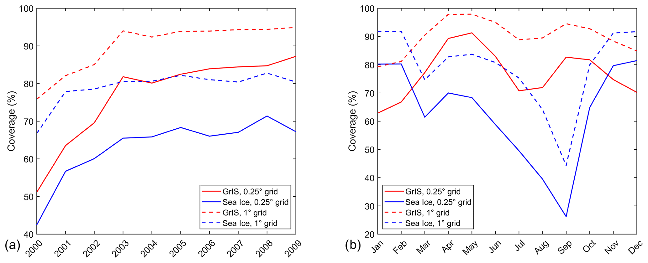
Figure 15 T2m_sat coverage averaged for (a) each year and (b) each month for the GrIS and sea ice, and using a grid resolution of 0.25^∘ and 1^∘, respectively.

As illustrated in Fig. 15, T2m_sat provides increasing coverage over the period 2000–2003 and quite stable coverage for the years 2003–2009. The average daily coverage is 84 % and 67 % for land ice and sea ice, respectively, for the stable 2003–2009 period and the 0.25^∘ grid. When considering a 1^∘ grid resolution, these numbers increase to 94 % and 81 %, respectively. Over land ice, the maximum coverage is during the spring and autumn, while the sea ice coverage has a clear drop in coverage during the summer due to increased cloud cover (Curry et al., 1996; Beesley and Moritz, 1999).

5 Discussion

Due to the limited number of in situ observations in the Arctic, and especially over sea ice, gathering in situ observations for testing and validating the regression models is not a simple task. The lack of observations that represent all conditions and regions in the Arctic and the resulting matching threshold of 15 km combined with the large topographical variations over the GrIS increase the uncertainty in the pixel-to-point comparison, thereby complicating the derivation and validation of the regression models. Despite this, the validation against independent in situ observations and the comparison with ERA-I and ERA5 demonstrate the value of the T2m_sat product in the Arctic.

Five regression models were tested, and the best regression model predicts T2m_sat from daily satellite IST_{skin_L3} combined with a seasonal variation. The performance of the T2m_sat product did not improve much when the wind speed information from ERA-I or ERA5 (Table 3) was included despite the fact that previous studies have shown a strong dependency of wind speed for both land ice and sea ice (Adolph et al., 2018; Hudson and Brandt, 2005; Miller et al., 2013; Nielsen-Englyst et al., 2019). This was unexpected, at least for sea ice. The reason is likely that the quality of the wind speed fields is not adequate for use in the relationship model. In particular, accurately representing katabatic winds in numerical weather prediction (NWP) models is a challenging task due to the high resolution needed in the vertical direction (Grisogono et al., 2007; Steeneveld, 2014; Weng and Taylor, 2003; Zilitinkevich et al., 2006). Furthermore, the representation of surface roughness and the processes of snow–surface coupling, radiation, and turbulent mixing are hampered by limited resolution, while the relative importance of the processes varies with wind speed (Sterk et al., 2013). More accurate information on the wind speed is expected to improve the performance of the regression model, which includes wind speed as a predictor. In particular, the higher-resolution NWP output may be very beneficial in the regions of the GrIS where the local topography interacts with the wind through katabatic effects (DuVivier and Cassano, 2013; Oltmanns et al., 2015; Renfrew, 2004). Regional high-resolution reanalysis products are currently being developed within the Copernicus Arctic regional Reanalysis service C3S project (https://climate.copernicus.eu/copernicus-arctic-regional-reanalysis-service, last access: 29 June 2021). It is likely that such products will provide winds that can be used within a relationship model.

Since infrared satellites cannot measure the surface temperature during cloudy conditions, a cold clear-sky bias is often observed in infrared satellite IST_{skin_L3} averages compared to all-sky temperature averages (see, e.g. Table 2; Hall et al., 2008; Koenig and Hall, 2010). When using satellite IST_{skin_L3} observations, it is thus important to be aware of the clear-sky bias, which moreover varies with different temporal averaging windows (Nielsen-Englyst et al., 2019). Here, when using an empirical statistical method, which is trained against daily averaged in situ T2m (obtained in both clear-sky and cloudy conditions), the conversion from IST_{skin_L3} to T2m_sat removes the systematic IST_{skin_L3} clear-sky bias effects that may be present in the satellite data. As a result, we obtain a T2m_sat estimate which performs similarly or better than the IST_{skin_L3}, when validated against in situ observations. For the IST_{skin_L3}, the temporal sampling errors resulting from clouds have been minimized through a number of requirements. For short-lasting (<24 h) cloudy conditions, the division into 3 h bin averages and the requirement of filled 3 h bins during both the night (between 18:00 and 06:00 LST) and day (between 06:00 and 18:00 LST) ensure that the diurnal cycle is best resolved despite the gaps with clouds. For long-lasting (≥24 h) cloudy conditions, IST_{skin_L3} is not available, and we do not retrieve T2m_sat for these days.

The T2m_sat product derived here provides increasing coverage over the period 2000–2003 and stable coverage for 2003–2009. The coverage varies with the season, with the minimum coverage over sea ice in the period from July to September due to extensive cloud cover over the Arctic sea ice during summer (Curry et al., 1996; Beesley and Moritz, 1999). Nevertheless, the average daily coverage is 84 % and 67 % for land ice and sea ice, respectively, for the stable 2003–2009 period. The high percentages in coverage demonstrate that the gaps due to cloudy days are limited (except for over sea ice in the summer) and that the dataset contains a significant amount of information on the all-sky daily T2m even though it is based on clear-sky satellite observations.

Atmospheric models using data assimilation or statistical techniques may be applied to fill in the gaps due to clouds. This has already been done in the EUSTACE project by using an advanced statistical model to combine in situ observed and clear-sky satellite-derived T2m estimates (over land, lakes, ocean, and ice), including uncertainty estimates, into a global and gap-free daily analysis of surface air temperatures from 1850 to 2015 (Morice et al., 2019; Rayner et al., 2020). The T2m_sat product derived in this paper is used as input to the EUSTACE surface air temperature analysis for the GrIS and the Arctic sea ice.

The T2m_sat dataset developed here only covers Arctic, but the AASTI satellite dataset also covers the Antarctica. This implies that similar statistical methods can be derived for the Antarctic ice sheet and sea ice. Preliminary investigations indicate that a T2m product can be derived for the Antarctic ice sheet with similar performance to GrIS, whereas the Southern Ocean sea ice is challenging due to very few in situ observations (Morice et al., 2012). For both southern regions, more in situ observations are needed to repeat the work performed for the Arctic and to determine a reliable statistical model. This product can also be extended to seasonal snow and ice, but it requires a dynamic surface mask and the derivation of the regression model to be repeated. However, similar efforts have already been made within EUSTACE to cover seasonal snow (Good, 2015; Morice et al., 2019; Rayner et al., 2020).

The AASTI version builds on the Clara version 1 dataset from the CM-SAF. A version 2 of the dataset is now available (Karlsson et al., 2017), which facilitates the production of an AASTI version 2 dataset that covers the period 1982 up to present. With consistency in the retrieval algorithm and datasets, it will be possible to use the relationship model to produce a satellite-based climate data record of T2m from 1982 to today.

Including other available satellite products such as MODIS IST observations (Hall et al., 2004) or the (A)ATSR dataset (Ghent et al., 2017) may improve the quality of the T2m_sat product. However, adding new data requires detailed knowledge of the characteristics of the dataset such as sampling frequency and uncertainty of the IST observations. In addition, determination of the relationship model is needed again. At the same time, adding more satellite overpasses to the daily estimates may not reduce the uncertainty of the products. This is evident when comparing Figs. 7 and 8 where the variation in the number of satellite observations during the record (Fig. 8) is not reflected in a similar variation in the performance of the product (Fig. 7). The uncertainty in the beginning of the record is comparable to the uncertainty at the end of the record, despite an almost doubling of the observed 3-hourly averages throughout the day.

6 Conclusions

The surface air temperature is one of the key indicators for Arctic climate change, and it can easily be compared with climate change indicators from other regions. This study introduces a methodology for using satellite skin temperatures for estimating air temperatures to compensate for the lack of in situ measurements and as a supplement to reanalysis products in the Arctic. Daily near-surface air temperatures (T2m) have been estimated based on daily clear-sky satellite Level 3 (L3) observations of ice surface skin temperatures (IST_{skin_L3}), using the Arctic and Antarctic ice Surface Temperatures from thermal Infrared satellite sensors (AASTI) reanalysis. A regression-based method has been used and tuned against in situ observed T2m using IST_{skin_L3} observations covering both Arctic sea ice and the Greenland Ice Sheet (GrIS). In general, there is a good correlation between T2m and IST_{skin_L3} due to the seasonal cycle in both IST and T2m. Different models have been tested to examine how to best capture the variability in the T2m–IST difference. The highest correlation and lowest RMSDs were found using a model where T2m_sat is predicted from daily satellite IST_{skin_L3} combined with a seasonal variation, assumed to have the shape of an annual harmonic. This model has been used to derive daily T2m on a 0.25^∘ regular latitude–longitude grid from the clear-sky AASTI IST_{skin_L3} over the Arctic during the time period 2000–2009 (Kennedy et al., 2019), using different regression coefficients for land ice and sea ice. Days with clouds or limited clear-sky observations have been excluded from the analysis. Considering a 1^∘ regular latitude–longitude grid, the average daily coverage of the T2m_sat product is 94 % over the GrIS and 81 % for sea ice for the years 2003–2009. The days when the T2m_sat is available, the T2m estimate can be considered a daily averaged all-sky T2m, since it has been tuned against all-sky in situ observations.

The estimated T2m_sat data show average biases of 0.30 and 0.35 ^∘C and average root-mean-square errors of 3.47 and 3.20 ^∘C for land ice and sea ice, respectively, when validated against independent in situ observations. All daily T2m_sat estimates include a total uncertainty estimate divided into a random, locally systematic, and large-scale systematic uncertainty component. The total uncertainty of T2m_sat shows good validation results when validated against independent in situ observations. A comparison with two of ECMWF's reanalyses (i.e. ERA-I and ERA5) shows that T2m_sat validates similarly or better than both of these even though the reanalyses actively assimilate available in situ observations. The T2m_sat product is independent of the quality of the NWP forecasts, and thus it represents an important supplement to the model-based T2m. The errors in NWP products (e.g. T2m_ERA-I or T2m_ERA5) and the errors in the product derived here (T2m_sat) are expected to be independent and uncorrelated, and a combination of a NWP product and the T2m_sat data can therefore lead to an even better T2m estimate. The regression models presented here both work on satellite observations that are available from reprocessed records but open up for a near-real-time estimation of T2m from satellites. The results obtained for the ice-covered areas show that there is a large potential for using satellite-observed surface temperatures to estimate near-surface air temperatures. These estimates are not supposed to replace the already existing air temperature measurements or reanalyses, but rather to supplement these in particular in areas where no in situ observations are currently available.