Impact of water vapor diffusion and latent heat on the effective thermal conductivity of snow

Heat transport in snowpacks is understood to occur through the two processes of heat conduction and latent heat transport carried by water vapor, which are generally treated as decoupled from one another. This paper investigates the coupling between both these processes in snow, with an emphasis on the impacts of the kinetics of the sublimation and deposition of water vapor onto ice. In the case when kinetics is fast, latent heat exchanges at ice surfaces modify their temperature and therefore the thermal gradient within ice crystals and the heat conduction through the entire microstructure. Furthermore, in this case, the effective thermal conductivity of snow can be expressed by a purely conductive term complemented by a term directly proportional to the effective diffusion coefficient of water vapor in snow, which illustrates the inextricable coupling between heat conduction and water vapor transport. Numerical simulations on measured three-dimensional snow microstructures reveal that the effective thermal conductivity of snow can be significantly larger, by up to about 50 % for low-density snow, than if water vapor transport is neglected. A comparison of our numerical simulations with literature data suggests that the fast kinetics hypothesis could be a reasonable assumption for modeling heat and mass transport in snow. Lastly, we demonstrate that under the fast kinetics hypothesis the effective diffusion coefficient of water vapor is related to the effective thermal conductivity by a simple linear relationship. Under such a condition, the effective diffusion coefficient of water vapor is expected to lie in the narrow 100 % to about 80 % range of the value of the diffusion coefficient of water vapor in air for most seasonal snows. This may greatly facilitate the parameterization of water vapor diffusion of snow in models.

1 Introduction

Thermal conductivity is one of the major physical properties of snow. It governs the magnitude of the thermal energy flux through the snowpack when subjected to a thermal gradient, and it thus plays an integral role in the energy budgets of the ground (Zhang et al., 1996), ice caps and glaciers (Gilbert et al., 2012), and sea ice (Lecomte et al., 2013), as well as in the temperature of the snow surface and therefore in meteorology (Domine et al., 2019). Moreover, variations of thermal conductivity between snow layers impact the temperature gradients at the layer scale and thus in part govern snow metamorphism (Vionnet et al., 2012). In light of its importance for the understanding of snow and environmental physics, snow thermal conductivity has been actively studied and measured for several decades (Yosida et al., 1955; Jaafar and Picot, 1970; Sturm and Johnson, 1992; Morin et al., 2010; Calonne et al., 2011; Riche and Schneebeli, 2013; Domine et al., 2015).

One of the peculiarities of snow is that energy transport does not solely occur through heat conduction. Indeed, when a snowpack is subjected to a thermal gradient, a macroscopic water vapor flux is also present (Sturm and Benson, 1997; Pinzer et al., 2012). This vapor flux carries latent heat in parallel to heat conduction. Several studies have investigated the influence of vapor transport on the total energy flux through snow under a thermal gradient. Among others, Sturm and Johnson (1992) report that the heat transport in snow is characterized by an effective thermal conductivity K^eff encompassing both the effects of heat conduction and vapor transport. In their framework, one can decompose the effective thermal conductivity as ${\mathbf{K}}^{\mathrm{eff}}={\mathbf{K}}^{\mathrm{cond}}+{\mathbf{K}}^{\mathrm{vap}}$, where K^cond is “the hypothetical conductivity in the absence of any vapor transport” (Sturm and Johnson, 1992) and K^vap corresponds to the latent heat transported with water vapor. In opposition to the idea of merging conduction and vapor transport in a single effective thermal conductivity, Calonne et al. (2011) “recommend purely conductive effects (i.e. conduction through ice and interstitial air) to be considered separately from non-conductive processes”, therefore treating heat conduction as decoupled from vapor transport.

The aim of this article is to provide a simplified analysis of the contribution of latent heat to the thermal energy flux in snow and notably to quantify the coupling between these processes at the macroscopic scale. For this we focus on two limiting cases, considering the kinetics of deposition and sublimation of water vapor to be either very fast or very slow. We start by providing theoretical considerations on the relationship between water vapor transport and the effective thermal conductivity. We then perform numerical simulations to quantify the contribution of latent heat to the effective thermal conductivity.

2 Theory

Let us consider a snow sample of volume V, subjected to a macroscopic thermal gradient denoted ∇T^M (potentially accompanied by a macroscopic vapor concentration gradient ∇C^M). We also make the simplifying assumption that convection in the pore space does not occur or can be neglected (similarly to Riche and Schneebeli, 2013; Calonne et al., 2014). Furthermore, let us assume that the sample is taken large enough to be larger than its representative elementary volume (REV; Auriault et al., 2010; Calonne et al., 2014). Moreover, we assume that the sample is small enough that it does not span several snow layers and that the macroscopic thermal and water vapor gradients can be considered constant over the sample. Under these conditions, the volume V of snow is representative of the entire snow layer, and both share the same physical properties. The existence of this intermediate size between the microscopic and macroscopic scales is guaranteed by the separation of scales between the microscopic and macroscopic descriptions, which is a necessary condition to treat snow as an equivalent homogeneous medium with well-defined physical properties (Auriault, 1991; Auriault et al., 2010). An illustration of the microscopic and macroscopic points of view and of the separation of scale between them is given in Fig. 1.

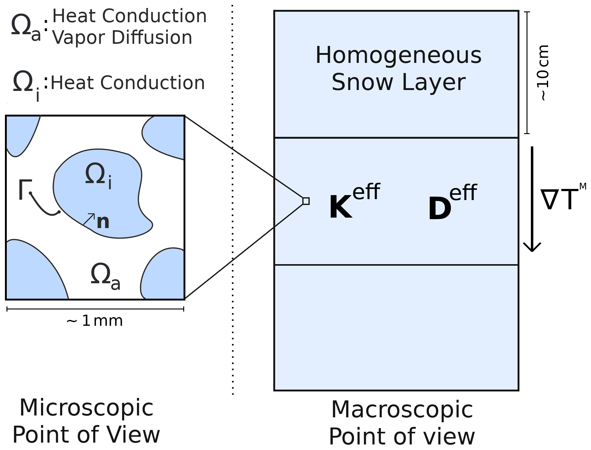
Figure 1 Illustration of the microscopic and macroscopic points of view of snow. At the microscopic scale, snow is composed of an ice space (Ω_i) and a pore space (Ω_a), separated by a boundary (Γ). Heat conduction occurs through the ice and pore spaces, while vapor diffusion is limited to the pore space. At the macroscopic scale, snow is treated as an equivalent homogeneous medium, with an effective thermal conductivity K^eff and an effective water vapor diffusion coefficient D^eff, and is subjected to a macroscopic thermal gradient ∇T^M.

The effective thermal conductivity K^eff of snow relates the macroscopic heat flux Q, transporting thermal energy at the macroscopic scale, to the thermal gradient ∇T^M with $\mathit{Q}=-{\mathbf{K}}^{\mathrm{eff}}\mathrm{\nabla }{T}^{\mathrm{M}}$ (e.g., Yosida et al., 1955; Sturm and Johnson, 1992; Riche and Schneebeli, 2013). Similarly, an effective vapor diffusion coefficient D^eff can be defined, which relates the macroscopic vapor flux F to the macroscopic concentration gradient ∇C^M with $\mathit{F}=-{\mathbf{D}}^{\mathrm{eff}}\mathrm{\nabla }{C}^{\mathrm{M}}$ (e.g., Shertzer and Adams, 2018; Fourteau et al., 2021). In snow sciences, it is usually expected that the effective thermal conductivity and vapor diffusion coefficient depends only on the snow microstructure and on the physical properties of the underlying materials (the ice and the air) but not on the macroscopic thermal and water vapor concentration gradients (Yosida et al., 1955; Jaafar and Picot, 1970; Sturm and Johnson, 1992; Colbeck, 1993; Morin et al., 2010; Calonne et al., 2011; Riche and Schneebeli, 2013; Domine et al., 2015). One should however keep in mind that it might not necessarily be true, depending on the nature of the mechanisms at play at the microscopic scale (for instance in the case of a dependence of the sticking coefficient of water molecules onto ice on the local saturation of water vapor, as discussed in Fourteau et al., 2021).

Finally, the effective thermal conductivity is represented by a 3×3 tensor. However, snow can be considered as a transverse isotropic material (Löwe et al., 2013), and this tensor is thus fully characterized by two scalar values, namely the vertical and horizontal thermal conductivities. These scalar values are respectively denoted $K_z^{\mathrm{eff}}$ and $K_{xy}^{\mathrm{eff}}$ in this article to differentiate them from the tensor. Similarly, D^eff is represented by a 3×3 tensor, but for snow it reduces to a horizontal component and a vertical component. Again, these scalar components are respectively denoted $D_z^{\mathrm{eff}}$ and $D_{xy}^{\mathrm{eff}}$. We define the normalized effective diffusion coefficient D^norm as ${\mathbf{D}}^{\mathrm{norm}}={\mathbf{D}}^{\mathrm{eff}}/D_{\mathrm{0}}$, where D₀ is the diffusion coefficient of water vapor in air. The definitions and symbols of the variables used for this work are summarized in Appendix A.

In this article, the effective thermal conductivity of snow will be obtained starting from the physics at the microscopic scale. The relevant microscopic physical mechanisms for heat transport are (i) heat conduction in the ice, (ii) heat conduction in the air, (iii) vapor diffusion in the air, and (iv) vapor deposition/sublimation at ice surfaces (Calonne et al., 2014). Moreover, we assume that the physics at the microscopic scale can be treated in a steady state. From our understanding this is justified as the timescale governing the microscopic scale is much shorter than the macroscopic timescale at which snow observations are made. Indeed, Hansen and Foslien (2015) report that the characteristic times at the macroscopic and microscopic scales differ by a factor of 10⁶. Consistent with this, Calonne et al. (2014) report that when expressed in a non-dimensional form, the time derivatives in the heat and mass equations are negligible compared to the flux terms. The microscopic equations governing energy and vapor transport are thus

$$\begin{array}{}\text{(1)}& \left\{\begin{array}{l}\mathrm{div}(-k_{\mathrm{i}}\mathrm{\nabla }{T}_{\mathrm{i}})=\mathrm{0}\left({\mathrm{\Omega }}_{\mathrm{i}}\right)\\ \mathrm{div}(-k_{\mathrm{a}}\mathrm{\nabla }{T}_{\mathrm{a}})=\mathrm{0}\left({\mathrm{\Omega }}_{\mathrm{a}}\right)\\ \mathrm{div}(-D_{\mathrm{0}}\mathrm{\nabla }c)=\mathrm{0}\left({\mathrm{\Omega }}_{\mathrm{a}}\right)\\ T_{\mathrm{i}}=T_{\mathrm{a}}\left(\mathrm{\Gamma }\right)\\ -k_{\mathrm{i}}\mathrm{\nabla }{T}_{\mathrm{i}}\cdot \mathit{n}=-k_{\mathrm{a}}\mathrm{\nabla }{T}_{\mathrm{a}}\cdot \mathit{n}-L{D}_{\mathrm{0}}\mathrm{\nabla }c\cdot \mathit{n}\left(\mathrm{\Gamma }\right)\\ -D_{\mathrm{0}}\mathrm{\nabla }c\cdot \mathit{n}=\mathit{\alpha }{v}_{\mathrm{kin}}(c-c_{\mathrm{sat}})\left(\mathrm{\Gamma }\right)\end{array}\right.,\end{array}$$

where Ω_i, Ω_a, Γ, and n represent the ice space, the pore space, the ice–pore interface, and the normal vector to Γ pointing toward the ice, respectively. The geometry of the microscopic problem is exemplified in Fig. 1. In Eq. (1), k_i and k_a are the thermal conductivities of ice and air, T_i and T_a are the ice and air temperatures, D₀ is the diffusion coefficient of vapor in the air, c is the concentration of vapor in the pores, c_sat is the saturation concentration of vapor at the ice interface, L is the latent heat of sublimation of ice, $v_{\mathrm{kin}}=\sqrt{\left(kT\right)/\left(\mathrm{2}\mathit{\pi }m\right)}$ is referred to as the kinetic velocity and is related to the velocity of water molecules in the gas phase (with k the Boltzmann's constant and m the mass of a water molecule), and α is a coefficient less than or equal to unity referred to as the sticking coefficient (or sometimes the accommodation coefficient) of water vapor molecules on ice surfaces. The last equation of the system is referred to as the Hertz–Knudsen equation, and it governs the sublimation and deposition of water molecules on the ice surfaces (Saito, 1996). The penultimate equation represents the impact of vapor sublimation/deposition on the continuity of the heat flux at the ice–pore interface. Finally, when a sufficiently large thermal gradient is imposed on a snow sample, the variations of c_sat due to differences in curvature of the ice surface become negligible compared to variations due to temperature differences (Colbeck, 1983). This large temperature gradient condition corresponds to the regime of temperature gradient metamorphism, usually observed for thermal gradients of 10 K m⁻¹ and above (Sommerfeld and LaChapelle, 1970; Colbeck, 1982). In this case, the saturation concentration of vapor can be treated as a function of the ice surface temperature only.

The system of Eq. (1) shows that there exists a two-way coupling between heat and vapor transport in snow. Indeed, the ice and air temperatures are impacted by the phase change in water vapor and the release/absorption of latent heat, while the water vapor concentration in the pores is impacted by temperature through the value of c_sat at the ice surfaces. This implies that the heat flux through a snow sample depends on the sublimation and deposition processes happening in the snow and that the magnitude of the coupling between the heat flux and the vapor transport depends on the kinetics of the adsorption and desorption of water molecules. This kinetics is encapsulated in the parameter α of the Hertz–Knudsen equation. A general treatment of the system of Eq. (1) in the case of an arbitrary α is however out of the scope of this article. In this work, we limit ourselves to two limiting cases, namely very slow (small α) and very fast (large α) surface kinetics. Moreover, we only focus on quantifying the energy and water vapor fluxes and their associated effective thermal conductivity and effective diffusion coefficient of vapor without deriving the complete macroscopic temperature and vapor equations (contrary to the work of Calonne et al., 2014, for instance). Finally, note that the notion of slow and fast kinetics is related to the notion of kinetics-limited (small α) and diffusion-limited (large α) metamorphism in snow (e.g.,  Krol and Löwe, 2016).

2.1 The slow kinetics case

In the slow kinetics case, we consider that α is sufficiently small that the sublimation/deposition of water vapor does not strongly impact the temperature field in the snow microstructure. In this case, the coupling between heat and water vapor can be neglected, and snow can be viewed as an inert medium for heat conduction. This slow kinetics case has been treated in detail by Calonne et al. (2011) and case 3 of Calonne et al. (2014). Here, the snow sample is characterized by an effective thermal conductivity ${\mathbf{K}}_{\mathrm{slow}}^{\mathrm{eff}}$ that only accounts for the heat conduction through the ice and the air as if the snow medium were inert for water vapor. The subscript slow, used in ${\mathbf{K}}_{\mathrm{slow}}^{\mathrm{eff}}$ and elsewhere in the paper, is used to emphasize the slow kinetics assumption. Calonne et al. (2011) showed that the effective thermal conductivity depends on the snow microstructure and on the ice and air thermal conductivities but not on the macroscopic thermal gradient. It can be obtained with microscale numerical simulations of heat conduction, which do not include vapor transport (e.g.,  Calonne et al., 2011; Riche and Schneebeli, 2013). Following a similar decomposition of the effective conductivity as that reported by Sturm and Johnson (1992), one has ${\mathbf{K}}_{\mathrm{slow}}^{\mathrm{eff}}={\mathbf{K}}_{\mathrm{slow}}^{\mathrm{cond}}$ and ${\mathbf{K}}_{\mathrm{slow}}^{\mathrm{vap}}=\mathrm{0}$. Note that the fact that ${\mathbf{K}}_{\mathrm{slow}}^{\mathrm{vap}}=\mathrm{0}$ does not imply that the vapor flux in snow is null. A macroscopic vapor flux might be present, but there is simply not enough mass that changes phase and release/absorption of latent heat to meaningfully impact the heat flux in the snow.

2.2 The fast kinetics case

In the fast kinetics case, α is sufficiently large that the adsorption/desorption of water molecules is fast enough to impose vapor saturation at the ice–air interface. Mathematically, this case can be treated by letting α→∞. While this mathematical treatment is purely theoretical (as α≤1), it helps in apprehending the effect of fast kinetics. This case corresponds to the diffusion-limited case, and the Hertz–Knudsen equation is replaced by the saturation of vapor at the ice–air interface. Moreover, it can be shown that in this case the vapor concentration equals its saturation value not only at the ice surface but also throughout the entire pore space (see Yosida et al., 1955, or Fourteau et al., 2021, for demonstrations). The system of Eq. (1) can therefore be rewritten as

$$\begin{array}{}\text{(2)}& \left\{\begin{array}{l}\mathrm{div}(-k_{\mathrm{i}}\mathrm{\nabla }{T}_{\mathrm{i}})=\mathrm{0}\left({\mathrm{\Omega }}_{\mathrm{i}}\right)\\ \mathrm{div}(-k_{\mathrm{a}}\mathrm{\nabla }{T}_{\mathrm{a}})=\mathrm{0}\left({\mathrm{\Omega }}_{\mathrm{a}}\right)\\ \mathrm{div}(-D_{\mathrm{0}}\mathrm{\nabla }{c}_{\mathrm{sat}})=\mathrm{0}\left({\mathrm{\Omega }}_{\mathrm{a}}\right)\\ T_{\mathrm{i}}=T_{\mathrm{a}}\left(\mathrm{\Gamma }\right)\\ -k_{\mathrm{i}}\mathrm{\nabla }{T}_{\mathrm{i}}\cdot \mathbf{n}=-k_{\mathrm{a}}\mathrm{\nabla }{T}_{\mathrm{a}}\cdot \mathbf{n}-L{D}_{\mathrm{0}}\mathrm{\nabla }{c}_{\mathrm{sat}}\cdot \mathbf{n}\left(\mathrm{\Gamma }\right)\end{array}\right..\end{array}$$

Using the chain rule, one has ∇c_sat=β∇T_a, where $\mathit{\beta }=\frac{\mathrm{d}{c}_{\mathrm{sat}}}{\mathrm{d}T}$. Re-injecting this equality into Eq. (2) yields

$$\begin{array}{}\text{(3)}& \left\{\begin{array}{l}\mathrm{div}(-k_{\mathrm{i}}\mathrm{\nabla }{T}_{\mathrm{i}})=\mathrm{0}\left({\mathrm{\Omega }}_{\mathrm{i}}\right)\\ \mathrm{div}(-k_{\mathrm{a}}\mathrm{\nabla }{T}_{\mathrm{a}})=\mathrm{0}\left({\mathrm{\Omega }}_{\mathrm{a}}\right)\\ \mathrm{div}(-\mathit{\beta }{D}_{\mathrm{0}}\mathrm{\nabla }{T}_{\mathrm{a}})=\mathrm{0}\left({\mathrm{\Omega }}_{\mathrm{a}}\right)\\ T_{\mathrm{i}}=T_{\mathrm{a}}\left(\mathrm{\Gamma }\right)\\ -k_{\mathrm{i}}\mathrm{\nabla }{T}_{\mathrm{i}}\cdot \mathbf{n}=-k_{\mathrm{a}}\mathrm{\nabla }{T}_{\mathrm{a}}\cdot \mathbf{n}-\mathit{\beta }L{D}_{\mathrm{0}}\mathrm{\nabla }{T}_{\mathrm{a}}\cdot \mathbf{n}\left(\mathrm{\Gamma }\right)\end{array}\right..\end{array}$$

Multiplying the third line by L and summing with the second line, one finally gets

$$\begin{array}{}\text{(4)}& \left\{\begin{array}{l}\mathrm{div}(-k_{\mathrm{i}}\mathrm{\nabla }{T}_{\mathrm{i}})=\mathrm{0}\left({\mathrm{\Omega }}_{\mathrm{i}}\right)\\ \mathrm{div}(-(k_{\mathrm{a}}+\mathit{\beta }L{D}_{\mathrm{0}}\left)\mathrm{\nabla }{T}_{\mathrm{a}}\right)=\mathrm{0}\left({\mathrm{\Omega }}_{\mathrm{a}}\right)\\ T_{\mathrm{i}}=T_{\mathrm{a}}\left(\mathrm{\Gamma }\right)\\ -k_{\mathrm{i}}\mathrm{\nabla }{T}_{\mathrm{i}}\cdot \mathbf{n}=-(k_{\mathrm{a}}+\mathit{\beta }L{D}_{\mathrm{0}})\mathrm{\nabla }{T}_{\mathrm{a}}\cdot \mathbf{n}\left(\mathrm{\Gamma }\right)\end{array}\right.,\end{array}$$

which is the system of equations governing the temperature and heat conduction in a microstructure without any explicit vapor transport and where the conductivity of the air has been replaced by an apparent conductivity k_v, defined as

$$\begin{array}{}\text{(5)}& k_{\mathrm{v}}=k_{\mathrm{a}}+\mathit{\beta }L{D}_{\mathrm{0}}.\end{array}$$

An equivalent demonstration of this result was proposed by Yosida et al. (1955). A similar result was also derived by Moyne et al. (1988) for a triphasic medium composed of water vapor, liquid water, and an inert solid phase, and it is consistent with the effective thermal conductivity model of soil proposed by De Vries (1958) and De Vries (1987).

As this system of equations is equivalent to the one of an inert medium with an increased air thermal conductivity, one can show using methods of homogenization (e.g., Auriault et al., 2010; Calonne et al., 2011) that at the macroscopic scale snow can be treated as an equivalent medium with a well-defined tensorial thermal conductivity ${\mathbf{K}}_{\mathrm{fast}}^{\mathrm{eff}}$. This effective thermal conductivity depends on the snow microstructure and on the physical properties of ice, air, and vapor (through k_i, k_a, and βLD₀) but not on the macroscopic thermal gradient. Again, the subscript fast is used to stress that we are working under the fast kinetics assumption.

We now investigate the individual contributions of conduction and vapor transport to ${\mathbf{K}}_{\mathrm{fast}}^{\mathrm{eff}}$. The macroscopic heat flux Q, which equals the volume average of the microscopic heat flux (Batchelor and Brien, 1977), can be decomposed as

$$\begin{array}{}\text{(6)}& \begin{array}{rl}\mathit{Q}& =-{\displaystyle \frac{\mathrm{1}}{V}}(\underset{V_{\mathrm{i}}}{\int }{k}_{\mathrm{i}}\mathrm{\nabla }{T}_{\mathrm{i}}\mathrm{d}V+\underset{V_{\mathrm{a}}}{\int }{k}_{\mathrm{v}}\mathrm{\nabla }{T}_{\mathrm{a}}\mathrm{d}V)\\ & =-(\mathrm{1}-\mathit{\varphi }){\displaystyle \frac{\mathrm{1}}{V_{\mathrm{i}}}}\underset{V_{\mathrm{i}}}{\int }{k}_{\mathrm{i}}\mathrm{\nabla }{T}_{\mathrm{i}}\mathrm{d}V-\mathit{\varphi }{\displaystyle \frac{\mathrm{1}}{V_{\mathrm{a}}}}\underset{V_{\mathrm{a}}}{\int }{k}_{\mathrm{a}}\mathrm{\nabla }{T}_{\mathrm{a}}\mathrm{d}V\\ & -\mathit{\varphi }{\displaystyle \frac{\mathrm{1}}{V_{\mathrm{a}}}}\underset{V_{\mathrm{a}}}{\int }\mathit{\beta }L{D}_{\mathrm{0}}\mathrm{\nabla }{T}_{\mathrm{a}}\mathrm{d}V\\ & =-(\mathrm{1}-\mathit{\varphi })k_{\mathrm{i}}<\mathrm{\nabla }{T}_{\mathrm{i}}>-\mathit{\varphi }{k}_{\mathrm{a}}<\mathrm{\nabla }{T}_{\mathrm{a}}>-\mathit{\varphi }\mathit{\beta }L{D}_{\mathrm{0}}\\ & <\mathrm{\nabla }{T}_{\mathrm{a}}>,\end{array}\end{array}$$

where V_i and V_a are the ice and air volumes in the snow, ϕ is the porosity, and $<\mathrm{\nabla }{T}_{\mathrm{i}}>$ and $<\mathrm{\nabla }{T}_{\mathrm{a}}>$ stand for the spatial averages of the thermal gradients in the individual ice and air spaces. Note that the average thermal gradient in the ice (respectively the air) is defined by performing the volume average in the ice space only (respectively the air space only) and not in the entire snow volume. The first two terms of the last line of Eq. (6) respectively correspond to the contribution of ice and air heat conduction to the energy flux, while the last term corresponds to an additional contribution of latent heat transported with water vapor. Moreover, recalling that with fast kinetics $\mathrm{\nabla }c=\mathrm{\nabla }{c}_{\mathrm{sat}}=\mathit{\beta }\mathrm{\nabla }{T}_{\mathrm{a}}$, the contribution of water vapor is given by

$$\begin{array}{}\text{(7)}& \begin{array}{rl}\mathit{\varphi }\mathit{\beta }L{D}_{\mathrm{0}}<\mathrm{\nabla }{T}_{\mathrm{a}}>& =L{\displaystyle \frac{\mathrm{1}}{V}}\underset{V_{\mathrm{a}}}{\int }\mathit{\beta }{D}_{\mathrm{0}}\mathrm{\nabla }{T}_{\mathrm{a}}\mathrm{d}V\\ & =L{\displaystyle \frac{\mathrm{1}}{V}}\underset{V_{\mathrm{a}}}{\int }{D}_{\mathrm{0}}\mathrm{\nabla }c\mathrm{d}V\\ & =L\mathit{F},\end{array}\end{array}$$

where $\mathit{F}=\frac{\mathrm{1}}{V}{\int }_{V_{\mathrm{a}}}{D}_{\mathrm{0}}\mathrm{\nabla }c\mathrm{d}V$ is the macroscopic vapor flux (Shertzer and Adams, 2018; Fourteau et al., 2021) which is linked to the macroscopic vapor gradient ∇C^M through an effective diffusion coefficient ${\mathbf{D}}_{\mathrm{fast}}^{\mathrm{eff}}$ such that $\mathit{F}=-{\mathbf{D}}_{\mathrm{fast}}^{\mathrm{eff}}\mathrm{\nabla }{C}^{\mathrm{M}}$ (Calonne et al., 2014; Fourteau et al., 2021). Since in the fast kinetics case vapor is at saturation throughout the pore space, the macroscopic vapor gradient is related to the macroscopic temperature gradient ∇T^M by ∇C^M=β∇T^M. Therefore, the macroscopic vapor flux is given by

$$\begin{array}{}\text{(8)}& \mathit{F}=-\mathit{\beta }{\mathbf{D}}_{\mathrm{fast}}^{\mathrm{eff}}\mathrm{\nabla }{T}^{\mathrm{M}}.\end{array}$$

The effective thermal conductivity of snow can thus be decomposed in

$$\begin{array}{}\text{(9)}& {\mathbf{K}}_{\mathrm{fast}}^{\mathrm{eff}}={\mathbf{K}}_{\mathrm{fast}}^{\mathrm{cond}}+\mathit{\beta }L{\mathbf{D}}_{\mathrm{fast}}^{\mathrm{eff}},\end{array}$$

where ${\mathbf{K}}_{\mathrm{fast}}^{\mathrm{cond}}$ is the contribution due to heat conduction in the ice and air, and $\mathit{\beta }L{\mathbf{D}}_{\mathrm{fast}}^{\mathrm{eff}}={\mathbf{K}}_{\mathrm{fast}}^{\mathrm{vap}}$ is the contribution of latent heat transported with water vapor. Contrary to the slow kinetics case, we now find that latent heat has an impact on the thermal properties of snow and that the vapor flux directly contributes to the effective thermal conductivity. A similar version of Eq. (9), with the contribution of vapor transport being $\mathit{\beta }L{\mathbf{D}}_{\mathrm{fast}}^{\mathrm{eff}}$, has notably been reported by Jordan (1991) and Sturm and Johnson (1992), which directly consider energy balance and transport at the macroscopic scale and pre-suppose the existence of well-defined (i.e., independent of the macroscopic thermal gradient) K^cond and D^eff.

It is important to note that ${\mathbf{K}}_{\mathrm{fast}}^{\mathrm{cond}}$ in Eq. (9) is different from the thermal conductivity when latent heat effects are neglected, i.e., ${\mathbf{K}}_{\mathrm{fast}}^{\mathrm{cond}}\ne {\mathbf{K}}_{\mathrm{slow}}^{\mathrm{cond}}$ (Moyne et al., 1988). Indeed, the heat conduction in the microstructure is determined by the distribution of the local thermal gradients in the two phases, and latent heat modifies the microscopic thermal gradients compared to the case without latent heat and thus modifies the heat conduction. The presence of latent heat increases the apparent thermal conductivity of the pore space and thus reduces the thermal conductivity contrast between the two phases. In turn, this reduced thermal contrast increases the average temperature gradient of the ice phase (the highly conducting phase) and decreases the average temperature gradient of the gas phase (the poorly conducting phase). The increase in heat conduction in the ice is larger than the decrease in the air, and the contribution of heat conduction alone is therefore greater with the presence of latent heat than without. Such an effect is illustrated and quantified with numerical simulations in Sect. 3.1.

Finally, we want to point out that in the fast kinetics case, the effective thermal conductivity and the effective water vapor diffusion coefficient are linearly related. Indeed, starting from the fact that the effective diffusion coefficient is given by the ratio of the magnitude of the vapor flux over the magnitude of the vapor concentration gradient, one has

$$\begin{array}{}\text{(10)}& \begin{array}{rl}{D}_{\mathrm{fast}}^{\mathrm{eff}}& ={\displaystyle \frac{\parallel \frac{\mathrm{1}}{V}{\int }_{V_{\mathrm{a}}}{D}_{\mathrm{0}}\mathrm{\nabla }c\mathrm{d}V\parallel }{\parallel \mathrm{\nabla }C\parallel }}={\displaystyle \frac{\parallel D_{\mathrm{0}}\mathit{\beta }\frac{\mathrm{1}}{V}{\int }_{V_{\mathrm{a}}}\mathrm{\nabla }{T}_{\mathrm{a}}\mathrm{d}V\parallel }{\parallel \mathit{\beta }\mathrm{\nabla }{T}^{\mathrm{M}}\parallel }}\\ & =D_{\mathrm{0}}{\displaystyle \frac{V_{\mathrm{a}}}{V}}{\displaystyle \frac{\parallel \frac{\mathrm{1}}{V_{\mathrm{a}}}{\int }_{V_{\mathrm{a}}}\mathrm{\nabla }{T}_{\mathrm{a}}\mathrm{d}V\parallel }{\parallel \mathrm{\nabla }{T}^{\mathrm{M}}\parallel }}=D_{\mathrm{0}}\mathit{\varphi }{\displaystyle \frac{\parallel <\mathrm{\nabla }{T}_{\mathrm{a}}>\parallel }{\parallel \mathrm{\nabla }{T}^{\mathrm{M}}\parallel }},\end{array}\end{array}$$

where we used the facts that ∇c=β∇T_a and ∇C^M=β∇T^M and where $D_{\mathrm{fast}}^{\mathrm{eff}}$ either stands for the vertical or for the horizontal effective diffusion coefficient depending on the orientation of the macroscopic thermal gradient. The ratio of the average thermal gradient in the pore space over the macroscopic thermal gradient is governed by the effective thermal conductivity and the thermal conductivity of the ice and the air. Indeed, we have

$$\begin{array}{}\text{(11)}& K_{\mathrm{fast}}^{\mathrm{eff}}\mathrm{\nabla }{T}^{\mathrm{M}}=(\mathrm{1}-\mathit{\varphi })k_{\mathrm{i}}<\mathrm{\nabla }{T}_{\mathrm{i}}>+\mathit{\varphi }{k}_{\mathrm{v}}<\mathrm{\nabla }{T}_{\mathrm{a}}>\end{array}$$

and

$$\begin{array}{}\text{(12)}& \mathrm{\nabla }{T}^{\mathrm{M}}=(\mathrm{1}-\mathit{\varphi })<\mathrm{\nabla }{T}_{\mathrm{i}}>+\mathit{\varphi }<\mathrm{\nabla }{T}_{\mathrm{a}}>,\end{array}$$

where similarly $K_{\mathrm{fast}}^{\mathrm{eff}}$ either stands for the vertical or for the horizontal effective thermal conductivity depending on the orientation of the macroscopic thermal gradient. Equation (11) follows from the definition of the macroscopic energy flux (Batchelor and Brien, 1977), and Eq. (12) follows from the application of Stokes theorem and has notably been previously reported by Hansen and Foslien (2015). Combining Eqs. (11) and (12) we have

$$\begin{array}{}\text{(13)}& \mathit{\varphi }<\mathrm{\nabla }{T}_{\mathrm{a}}>={\displaystyle \frac{k_{\mathrm{i}}-K_{\mathrm{fast}}^{\mathrm{eff}}}{k_{\mathrm{i}}-k_{\mathrm{v}}}}\mathrm{\nabla }{T}^{\mathrm{M}}.\end{array}$$

Finally, injecting Eq. (13) into Eq. (10) we have

$$\begin{array}{}\text{(14)}& D_{\mathrm{fast}}^{\mathrm{eff}}=D_{\mathrm{0}}{\displaystyle \frac{k_{\mathrm{i}}-K_{\mathrm{fast}}^{\mathrm{eff}}}{k_{\mathrm{i}}-k_{\mathrm{v}}}}.\end{array}$$

Since the effective thermal conductivity is larger than the conductivity of the least conducting phase, i.e., $K_{\mathrm{fast}}^{\mathrm{eff}}>k_{\mathrm{v}}$, one finds that $D_{\mathrm{fast}}^{\mathrm{eff}}\le D_{\mathrm{0}}$, as reported by Giddings and LaChapelle (1962) and Fourteau et al. (2021). The linear relationship between the effective thermal conductivity and the normalized effective water vapor diffusion coefficient at 263 K is displayed in Fig. 2 for effective thermal conductivities $K_{\mathrm{fast}}^{\mathrm{eff}}$ ranging from k_v=0.0336 to $\mathrm{0.5}\mathrm{W}{\mathrm{K}}^{-\mathrm{1}}{\mathrm{m}}^{-\mathrm{1}}$, as typically encountered with seasonal snow (e.g.,  Sturm et al., 1997; Calonne et al., 2011; Riche and Schneebeli, 2013, and the numerical values computed in Sect. 3.2 of this paper). The application of Eq. (14) in Fig. 2 reveals that the normalized effective diffusion coefficient ranges from 1 to about 0.8 for most seasonal snow. Moreover, as the macroscopic vapor flux decreases with slower kinetics (Pinzer et al., 2012; Fourteau et al., 2021), this curve represents an upper limit for the effective diffusion coefficient.

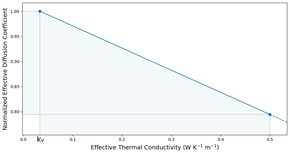
Figure 2 Normalized effective water vapor diffusion coefficient as a function of the effective thermal conductivity under the fast kinetics hypothesis at 263 K. The shaded area covers the typical range of thermal conductivity values (from k_v up to $\mathrm{0.5}\mathrm{W}{\mathrm{K}}^{-\mathrm{1}}{\mathrm{m}}^{-\mathrm{1}}$) and the corresponding range of the normalized effective diffusion coefficient of water vapor (from 1 to about 0.8). At 263 K, $k_{\mathrm{v}}=k_{\mathrm{a}}+\mathit{\beta }L{D}_{\mathrm{0}}=\mathrm{0.0336}\mathrm{W}{\mathrm{K}}^{-\mathrm{1}}{\mathrm{m}}^{-\mathrm{1}}$.

2.3 Intermediate cases

Numerous works indicate that α depends on temperature, the local vapor saturation, and the crystallographic properties of the underlying ice surface (e.g., Saito, 1996; Libbrecht and Rickerby, 2013), but for snow it remains unclear what value or expression should be used for α in the Hertz–Knudsen equation (Legagneux and Domine, 2005). However, a recent study suggests that the very slow kinetics and fast surface kinetics cases correspond to the minimum and maximum macroscopic vapor diffusion in snow, respectively (Fourteau et al., 2021). We can therefore expect the energy flux Q to be maximal in the fast kinetics case since this corresponds to the situation with maximal vapor flux and the fastest adsorption and desorption of water molecules onto the ice surface. Similarly, the energy flux is minimal in the slow kinetics case as latent heat effects are absent in this case. The energy flux in snow Q can thus be bounded by the slow kinetics and the fast kinetics cases:

$$\begin{array}{}\text{(15)}& K_{\mathrm{slow}}^{\mathrm{eff}}\parallel \mathrm{\nabla }{T}^{\mathrm{M}}\parallel \le Q\le K_{\mathrm{fast}}^{\mathrm{eff}}\parallel \mathrm{\nabla }{T}^{\mathrm{M}}\parallel ,\end{array}$$

where this inequality applies both for the vertical and horizontal components of the effective thermal conductivities, depending on the orientation of the macroscopic thermal gradient.

3 Numerical simulations

To exemplify and quantify the points raised in Sect. 2, we performed finite element simulations of steady-state thermal conduction through several snow microstructures obtained experimentally with computed microtomography. The simulations were performed using the open-source Elmer FEM software (Malinen and Råback, 2013) and the readily available solver for the heat equation.

In each simulation, the temperatures of two opposite sides of the microstructure were imposed in order to obtain a thermal gradient of 50 K m⁻¹, with adiabatic conditions on the remaining sides. Similarly to Riche and Schneebeli (2013), the effective thermal conductivities are estimated by computing the ratio of the macroscopic heat flux Q to the macroscopic thermal gradient ∇T^M. The macroscopic heat flux Q is computed as the volume average of the microscopic heat fluxes using the ParaView software. Note that the chosen value of 50 K m⁻¹ for the imposed gradient is purely arbitrary and does not have an impact on our results as the resulting effective thermal conductivity does not depend on the magnitude of the gradient.

In order to test the influence of temperature on the effective thermal conductivity of snow, the simulations were run for different mean temperatures, ranging from 223 to 273 K. The temperature dependence of the thermal conductivities of ice and air (k_i and k_a) were respectively taken from Lide (2006) (based on  Slack, 1980) and Kadoya et al. (1985). The parameter $\mathit{\beta }=\frac{\mathrm{d}{c}_{\mathrm{sat}}}{\mathrm{d}T}$ was obtained by assuming that water vapor follows the Clausius–Clapeyron and ideal gas laws (Eq. 11 of Fourteau et al., 2021). We set the diffusion coefficient of water vapor in air to $D_{\mathrm{0}}=\mathrm{2}\times {\mathrm{10}}^{-\mathrm{5}}{\mathrm{m}}^{\mathrm{2}}{\mathrm{s}}^{-\mathrm{1}}$ (Calonne et al., 2014) and the latent heat of sublimation of ice $L=\mathrm{28}\times {\mathrm{10}}^{\mathrm{5}}\mathrm{J}{\mathrm{kg}}^{-\mathrm{1}}$ (Lide, 2006), independent of temperature. Finally, we assume that the density of ice ρ_ice is constant with temperature and equal to 917 kg m⁻³ (Calonne et al., 2014). The densities of the samples reported in this article are computed using ρ_ice, and the ice volume fractions are deduced from the tomography images.

For the different microstructures and mean temperatures, two types of simulations were performed, one in which we assumed no impact of latent heat on the heat conduction (thus obtaining ${\mathbf{K}}_{\mathrm{slow}}^{\mathrm{eff}}$), and the other in which we increased the apparent thermal conductivity of air by a βLD₀ term (thus obtaining ${\mathbf{K}}_{\mathrm{fast}}^{\mathrm{eff}}$). Moreover, as seen in Sect. 2.2 with Eq. (14), under the fast kinetics assumption the effective diffusion coefficient of water vapor ${\mathbf{D}}_{\mathrm{fast}}^{\mathrm{eff}}$ can be directly obtained from the effective thermal conductivity. Finally, we recall that the normalized effective diffusion coefficient is defined as the ratio of the effective diffusion coefficient with the diffusion coefficient of water vapor in free air, i.e., ${\mathbf{D}}^{\mathrm{norm}}={\mathbf{D}}^{\mathrm{eff}}/D_{\mathrm{0}}$.

In total we used 34 measured snow microstructures covering several types of seasonal snow. The particular snow types used are, according to the terminology of Fierz et al. (2009), precipitation particles (PP), decomposing and fragmented precipitation particles (DF), rounded grains (RG), faceted crystals (FC), depth hoar (DH), and melt forms (MF). We used sample sizes larger than the REV sizes reported by Calonne et al. (2011). The tetrahedral meshes used in the finite element simulations were produced using the Computational Geometry Algorithms Library (CGAL) and contain between 20 and 90 million elements. The samples are described in the Supplement and include both previously published snow samples (from Hagenmuller et al., 2016, 2019; Peinke et al., 2020) and new snow samples.

3.1 Effect of temperature on the effective thermal conductivity

In this section we analyze the influence of the mean temperature on the effective thermal conductivity. For simplicity, we limit ourselves to vertical temperature gradients and thus only deal with vertical effective thermal conductivities and vertical diffusion coefficients of water vapor. As all scalar components are vertical, we do not use the subscript z in order to lighten the notation.

The temperature dependence of K^eff is due to the temperature dependence of the underlying materials. Indeed, an increasing temperature results in the decrease in the ice thermal conductivity k_i and the increase in the apparent thermal conductivity of the air k_v due to both the increase in the intrinsic thermal conductivity of air k_a and the increase in the contribution of water vapor latent heat βLD₀, all displayed in Fig. 3.

Furthermore, we define for our analysis

$$\begin{array}{}\text{(16)}& \begin{array}{rl}& K^{\mathrm{ice}}=(\mathrm{1}-\mathit{\varphi })k_{\mathrm{i}}{\displaystyle \frac{\parallel <\mathrm{\nabla }{T}_{\mathrm{i}}>\parallel }{\parallel \mathrm{\nabla }T\parallel }},\\ & K^{\mathrm{air}}=\mathit{\varphi }{k}_{\mathrm{a}}{\displaystyle \frac{\parallel <\mathrm{\nabla }{T}_{\mathrm{a}}>\parallel }{\parallel \mathrm{\nabla }T\parallel }},\end{array}\end{array}$$

where K^ice (not to be mistaken with k_i; see Appendix A) corresponds to the contribution of the ice heat conduction to the total effective thermal conductivity and K^air (not to be mistaken with k_a) to the contribution of the air heat conduction. We have by construction

$$\begin{array}{}\text{(17)}& K^{\mathrm{cond}}=K^{\mathrm{ice}}+K^{\mathrm{air}},\end{array}$$

where K^cond is the vertical component of K^cond. With our simulations, the values of K^cond, K^ice, and K^air are computed directly from K^eff, k_i, k_a, and k_v and using Eqs. (11) and (12).

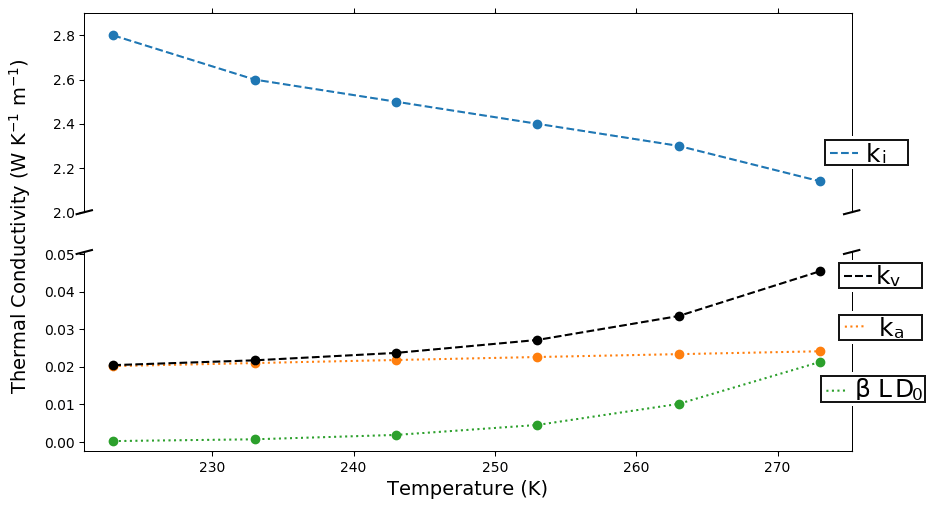
Figure 3 Temperature dependence of the thermal conductivity of ice (k_i in blue), of the thermal conductivity of air (k_a in orange), of the contribution of latent heat to the apparent thermal conductivity of the air (βLD₀ in green), and of the apparent thermal conductivity of air including latent heat effect ($k_{\mathrm{v}}=k_{\mathrm{a}}+\mathit{\beta }L{D}_{\mathrm{0}}$ in black). Note the break in the y axis.

We first focus on only two snow samples: a low-density sample and a high-density sample. The low-density sample is composed of decomposing and fragmented precipitation particles (DF) with a density of 125 kg m⁻³ and a specific surface area of 40 m² kg⁻¹. The high-density sample is composed of melt forms (MF) with a density of 380 kg m⁻³ and a specific surface area of 5 m² kg⁻¹. The three-dimensional microstructures of both samples are displayed in Fig. 4. The results of the finite element simulations for these two samples are reported in Fig. 5.

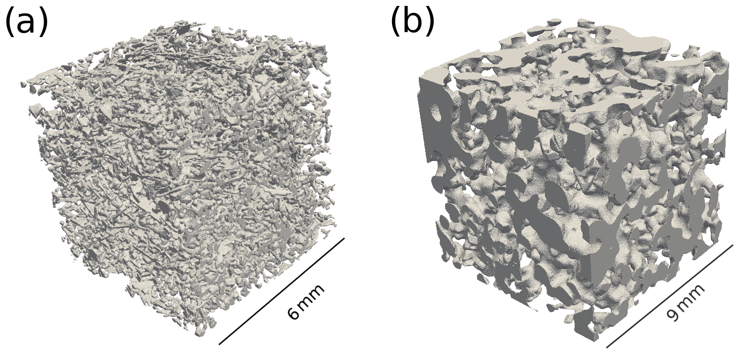
Figure 4 Tetrahedral meshes (ice phase only) of the low-density DF sample (a) and high-density MF sample (b).

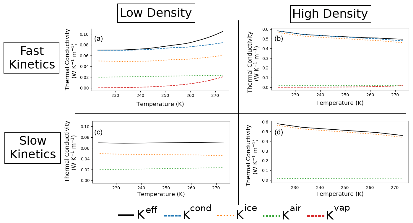
Figure 5 Vertical effective thermal conductivity (K^eff), with the contributions of ice heat conduction (K^ice), air heat conduction (K^air), and vapor transport (K^vap) for a low-density snow sample (a, c) and a high-density snow sample (b, d), as well as in the fast (upper line) and slow (lower line) kinetics cases. K^cond stands for the purely conductive part of K^eff and is given by $K^{\mathrm{cond}}=K^{\mathrm{ice}}+K^{\mathrm{air}}$.

We start by analyzing the low-density sample (left column of Fig. 5). Under the fast kinetics hypothesis, the effective thermal conductivity of the low-density sample shows an exponential-like increase with increasing temperature. This increase in K^eff is due to the combined effects of (i) an increase in K^vap, the vertical component of the contribution of latent heat transport, and (ii) an increase in K^cond, the heat conduction through the ice and air spaces. The increase in K^cond is principally due to the increase in K^ice, the heat conduction in the ice. With increasing temperature, the increase in the apparent thermal conductivity of air reduces the contrast between the two phases, and the average ice thermal gradient increases. This increase more than offsets the decrease in the ice thermal conductivity k_i, and the net effect is an increase in K^ice. Under the slow kinetics hypothesis, however, the effective thermal conductivity only barely decreases over the range of temperature studied, consistent with the results of Calonne et al. (2011). In this case, the increase in the thermal conductivity of the air is not as pronounced, and the increase in the thermal gradient in the ice does not compensate for the decrease in the ice thermal conductivity. Overall K^ice decreases with temperature in the slow kinetics case.

Contrary to the low-density sample, the high-density sample (right column of Fig. 5) shows a decrease in the effective thermal conductivity in the fast kinetics case. The increase in K^vap with temperature does not counter the decrease in K^cond. This decrease in K^cond can be attributed to the decrease in K^ice with temperature. Here, the increase in the ice thermal gradient is not large enough to offset the decrease in the ice thermal conductivity k_i, and overall K^ice decreases. Under the slow kinetics hypothesis, the effective thermal conductivity of the high-density sample decreases with temperature slightly more rapidly than in the fast kinetics case.

For both samples, the difference between $K_{\mathrm{slow}}^{\mathrm{eff}}$ and $K_{\mathrm{fast}}^{\mathrm{eff}}$ is maximal near the melting point, where it reaches more than 50 % for low-density snow. Moreover, neglecting the effect of water vapor transport on heat conduction under the fast kinetics case can lead to an underestimation of about 20 % of the conduction contribution. Thus in the fast kinetics case, the effect of latent heat can only reasonably be neglected for low temperatures or high-density samples.

In order to better quantify the difference between the fast and slow kinetics cases, we computed the vertical effective thermal conductivity for the totality of our 34 snow samples under both hypotheses, at 248 and 273 K. The ratios of the effective thermal conductivity in the fast kinetics case over the slow kinetics case are displayed in Fig. 6. They confirm that the relative difference is more important for low-density snow and for higher temperatures. Near the melting point (Fig. 6b), the fast kinetics effective thermal conductivity is between 10 % and 50 % higher than in the slow kinetics case. For colder snow at 248 K (Fig. 6a), the relative difference is less marked and ranges from 1 % to 10 %. When expressed in absolute terms, however, the difference between the fast and slow kinetics thermal conductivity is more marked for high-density snow.

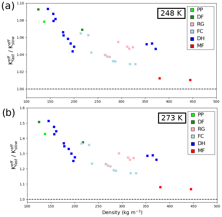
Figure 6 Ratio of the fast kinetics over the slow kinetics vertical effective thermal conductivity for various snow samples as a function of density. Computations performed at 248 K in (a) and 273 K in (b). Note the different y-axis scales in both panels.

Finally, Fig. 7 shows the variation of the vertical normalized effective diffusion coefficient of water vapor with temperature under the fast kinetics hypothesis and for the low and high-density samples shown in Fig. 4. The numerical values are consistent with the recent study of Fourteau et al. (2021), who obtained effective diffusion coefficients using finite element simulations explicitly representing vapor diffusion in the pores. Figure 7 reveals a slight decrease in the effective diffusion coefficient with temperature for both low- and high-density snow. This can be explained by the decrease in the air thermal gradient as the apparent conductivity of air increases with temperature. A lower air temperature gradient leads to a lower vapor concentration gradient in the pores and thus to a lower vapor flux and a lower $D_{\mathrm{fast}}^{\mathrm{norm}}$.

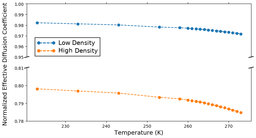
Figure 7 Vertical normalized effective diffusion coefficient $D_{\mathrm{fast}}^{\mathrm{norm}}$ of a low-density snow sample (blue) and a high-density snow sample (orange) as a function of temperature and under the hypothesis of fast kinetics. Note the break in the y axis.

3.2 Effective thermal conductivity and diffusion coefficient as a function of snow density

The slow kinetics effective thermal conductivities of snow samples covering a broad range of densities and microstructures have been reported by Calonne et al. (2011) and Riche and Schneebeli (2013). Similarly, numerical values of the effective diffusion coefficient of water vapor in snow under limited kinetics have been provided by Calonne et al. (2014). Here, we provide numerical estimates of the effective thermal conductivities and effective diffusion coefficients of a broad range of snow samples, this time under the fast kinetics hypothesis. For each sample we computed the vertical and horizontal effective thermal conductivities and water vapor effective diffusion coefficients, at five different temperatures (223, 248, 263, 268, and 273 K). The thermal conductivities and diffusion coefficients of each simulated sample are available in the Supplement.

The thermal conductivities computed at 263 K are displayed in Fig. 8 as a function of density. Similar to the work of Calonne et al. (2011) and Riche and Schneebeli (2013), we observe that density and thermal conductivity are well correlated, with denser snow samples presenting higher thermal conductivity values. For the low-density samples, for which the conduction of air plays a determinant role in the effective thermal conductivity, we report thermal conductivity values higher than the polynomial fits of Calonne et al. (2011) and Riche and Schneebeli (2013), both based on the slow kinetics hypothesis. This difference can be explained by the increased apparent thermal conductivity of the air due to latent heat effects. At higher density, our data lie above the reported data and polynomial fit of Calonne et al. (2011). As the relative difference between the fast and slow kinetics cases is small for high-density samples, one can expect the slow and fast kinetics simulations to yield similar values for high-density samples. The scatter between our values and the study of Calonne et al. (2011) is likely due to the inherent variability between snow samples, even for equal densities. Note that the fit proposed by Riche and Schneebeli (2013) was based on faceted crystals and depth hoar snow only and at 253 K. On the contrary the fit proposed by Calonne et al. (2011) was based on their entire sample set at 271 K.

Figure 8 Effective thermal conductivity of snow as a function of density under the fast kinetics assumption at 263 K. The horizontal bar of a symbol marks the horizontal effective thermal conductivity value of a snow sample, while the tip of the vertical bar marks its vertical value. Snow classification according to Fierz et al. (2009). Black dot: apparent thermal conductivity of air at 263 K. Solid black line: second-order polynomial fit of the vertical effective thermal conductivity. Dashed grey line: polynomial fit proposed by Calonne et al. (2011) under the slow kinetics assumption at 271 K. Dotted grey line: polynomial fit proposed by Riche and Schneebeli (2013) under the slow kinetics assumption at 253 K.

We adjusted second-order polynomial functions to derive parameterizations of thermal conductivity as a function of density and this for each of the five temperatures studied. Our parametrization for the vertical effective thermal conductivity at 263 K is displayed as a solid line in Fig. 8. The parameterizations of the vertical effective thermal conductivity for the five different temperatures are given by

$$\begin{array}{}\text{(18)}& K_z^{\mathrm{eff}}=\left\{\begin{array}{ll}\mathrm{2.564}(\frac{\mathit{\rho }}{{\mathit{\rho }}_{\mathrm{ice}}}{)}^{\mathrm{2}}-\mathrm{0.059}\frac{\mathit{\rho }}{{\mathit{\rho }}_{\mathrm{ice}}}+\mathrm{0.0205}& \mathrm{for}T=\mathrm{223}\mathrm{K}\\ \mathrm{2.172}(\frac{\mathit{\rho }}{{\mathit{\rho }}_{\mathrm{ice}}}{)}^{\mathrm{2}}+\mathrm{0.015}\frac{\mathit{\rho }}{{\mathit{\rho }}_{\mathrm{ice}}}+\mathrm{0.0252}& \mathrm{for}T=\mathrm{248}\mathrm{K}\\ \mathrm{1.985}(\frac{\mathit{\rho }}{{\mathit{\rho }}_{\mathrm{ice}}}{)}^{\mathrm{2}}+\mathrm{0.073}\frac{\mathit{\rho }}{{\mathit{\rho }}_{\mathrm{ice}}}+\mathrm{0.0336}& \mathrm{for}T=\mathrm{263}\mathrm{K}\\ \mathrm{1.883}(\frac{\mathit{\rho }}{{\mathit{\rho }}_{\mathrm{ice}}}{)}^{\mathrm{2}}+\mathrm{0.107}\frac{\mathit{\rho }}{{\mathit{\rho }}_{\mathrm{ice}}}+\mathrm{0.0386}& \mathrm{for}T=\mathrm{268}\mathrm{K}\\ \mathrm{1.776}(\frac{\mathit{\rho }}{{\mathit{\rho }}_{\mathrm{ice}}}{)}^{\mathrm{2}}+\mathrm{0.147}\frac{\mathit{\rho }}{{\mathit{\rho }}_{\mathrm{ice}}}+\mathrm{0.0455}& \mathrm{for}T=\mathrm{273}\mathrm{K}\end{array}\right.,\end{array}$$

where $\frac{\mathit{\rho }}{{\mathit{\rho }}_{\mathrm{ice}}}$ is the volume fraction of ice, and the constant terms in the polynomial equations correspond to k_v. Similar parameterizations for the horizontal thermal conductivity and for the geometric mean of the vertical and horizontal thermal conductivities are available in the Supplement of this article. This parametrization can be extended to other temperatures by first computing the thermal conductivity at the desired density for the five proposed temperatures and then performing an interpolation to the desired temperature.

Figure 9 Temperature dependence of the vertical effective thermal conductivity parameterizations under the fast kinetics hypothesis.

These vertical effective thermal conductivity parameterizations, displayed in Fig. 9, show a decrease in the slopes of the thermal conductivity versus density curves with increasing temperatures. This is consistent with the observations made in Sect. 3.1 that the thermal conductivity of the low-density sample increases with temperature, while the thermal conductivity of the high-density sample decreases with temperature. The transition between these two behaviors lies around 350 to 400 kg m⁻³. Note that Calonne et al. (2019) report that a similar transition between the low- and high-density samples also exists under limited kinetics but occurs at a much lower density of about 100 kg m⁻³.

Figure 10 Normalized effective diffusion coefficient as a function of density under the fast kinetics assumption at 263 K. Snow classification according to Fierz et al. (2009). Solid black line: normalized effective diffusion coefficient deduced from the application of Eq. (14) with the effective thermal conductivity polynomial fit of Fig. 8.

Finally, the estimated normalized effective diffusion coefficients of water vapor are displayed in Fig. 10 as a function of density at 263 K. The normalized effective diffusion coefficients obtained by application of Eq. (14), together with the polynomial fit of the vertical effective thermal conductivity, are shown as a solid black line in Fig. 10. The normalized effective diffusion coefficient decreases with density and mostly remains in the 0.98 to 0.8 range. Notably, detailed seasonal snow models working under the fast kinetics assumption could thus make the reasonable simplifying assumption that D^norm=0.90, independent of snow type. This would result in a less than 10 % error on the effective diffusion coefficient of water vapor.

4 Discussion

4.1 Does the fast kinetics hypothesis apply for heat and mass transport in snow?

This paper studied two limiting cases, considering either that the kinetics of water vapor deposition/sublimation is sufficiently fast to impose saturated water vapor at the ice interface (very large α) or that the kinetics is sufficiently slow so that latent heat does not have an impact on either the temperature gradients or the heat conduction in the snow microstructure (very small α). It remains however unclear if one of these two limiting cases applies for snow modeling. For example, based on the observation of snow crystal growth with computed tomography, Krol and Löwe (2016) suggest that isothermal metamorphism is slightly better represented by a slow kinetics, while temperature gradient metamorphism data appear consistent with fast kinetics.

As seen in Sect. 3.1, the effective thermal conductivity of low-density snow displays a fundamentally different dependence on temperature depending on whether the slow or the fast kinetics hypothesis applies. In the slow kinetics case, the effective thermal conductivity slightly decreases with increasing temperature, while it increases in the fast kinetics case. Using the needle probe method, Sturm and Johnson (1992) measured the variation of the effective thermal conductivity of a low-density sample of depth hoar with temperature. Even though recent studies have highlighted a potential bias of the needle probe method when used with snow (Calonne et al., 2011; Riche and Schneebeli, 2013), this reported bias does not have an impact on the trend of thermal conductivity measured at different temperatures in similar snow samples, as performed by Sturm and Johnson (1992). These data can thus be expected to reflect the variation of the effective thermal conductivity with temperature. These measurements, displayed in Fig. 7 of Sturm and Johnson (1992), clearly indicate an exponential-like increase in thermal conductivity with temperature, consistent with the fast kinetics hypothesis but not with the slow kinetics hypothesis.

The differences between the slow and fast kinetics cases on the effective diffusion coefficient of water vapor were also studied by Fourteau et al. (2021). While direct measurements of the effective diffusion coefficient are difficult and should therefore be analyzed with caution, the reported experimental values of Sokratov and Maeno (2000) report an average normalized diffusion coefficient of 0.64 for snow densities of about 475 kg m⁻³, while Calonne et al. (2014) report a value of about 0.35 for limited kinetics, and extrapolation of our results suggests a value of about 0.70 under the fast kinetics. Finally, the numerical simulations of Fourteau et al. (2021) indicate that for water vapor diffusion the transition between the slow and fast kinetics regimes occurs for sticking coefficients α around 10⁻³. Based on data by Libbrecht (2006), Kaempfer and Plapp (2009) report that α is likely to be within the 10⁻³ to 10⁻¹ range, thus within the fast kinetics regime.

All the above reasons suggest that the effective thermal conductivity and diffusion coefficient of water vapor in snow could be well represented under the fast kinetics hypothesis, at least during temperature gradient metamorphism. Further experimental work should be performed to confirm that the fast kinetics assumption generally applies for modeling mass and heat transport in snow and to highlight its potential limitations. Also, the derivation of a theoretical model able to describe heat and mass transfer with arbitrary surface kinetics would allow one to investigate intermediate kinetics in an effort to ultimately select the best modeling assumptions for snow. At the same time, this model could be formulated to explicitly take into account macroscopic convection as this phenomenon has been observed in sub-arctic shallow snowpacks (Trabant and Benson, 1972; Sturm and Johnson, 1991). Its derivation could be achieved using standard homogenization methods, such as the two-scale asymptotic expansion (e.g., Municchi and Icardi, 2020) or volume averaging methods (e.g., Whitaker, 1977).

4.2 The coupling of heat conduction with vapor transport

We showed that in the fast kinetics case, the pure conduction part K^cond of the effective thermal conductivity is influenced by the presence of water vapor and its latent heat. Therefore, the definition of K^cond given by Sturm and Johnson (1992), i.e., that it is “the hypothetical conductivity in the absence of any vapor transport”, should be clarified to emphasize that K^cond corresponds to the pure conduction occurring through the ice and pore spaces but in response to the actual microscopic thermal gradients that are influenced by the latent heat effects. Furthermore, the dependence of the pure conduction part on temperature is different from what would be expected from variations of the ice and air thermal conductivity only. This means that under the fast kinetics hypothesis a strong two-way coupling exists between heat conduction and water vapor transport, and the heat conduction process cannot be fully considered without latent heat processes. One should therefore be careful when treating heat conduction as decoupled from vapor transport (e.g., Calonne et al., 2011; Riche and Schneebeli, 2013). While this approximation is justified if the effects of latent heat are small, one should be aware of the potential limit of this approximation. Finally, in such a case it is not possible to experimentally decouple the measurement of K^cond from K^vap by performing measurements at low temperature (where K^vap≃0). The inferred value of K^cond at low-temperature does not hold at higher temperatures, at which the effect of latent heat is no longer negligible and thus has an impact on K^cond. A similar conclusion was reached by Moyne et al. (1988) for the thermal conductivity of a humid triphasic medium.

5 Conclusions

This paper investigates the effective thermal conductivity of snow and its relationship to the diffusion of water vapor and its associated latent heat. Using theory, we show that the kinetics of the sublimation and deposition processes at the ice surfaces plays a significant role on the transport of heat in snow. In particular, if the kinetics is slow, we recall that snow can be treated as an inert medium and that heat transport only occurs through conduction in the ice and in the air. In contrast, if the kinetics is fast, vapor transport and latent heat effects become an integral part of heat transport, and the effective thermal conductivity of snow is composed of a purely conductive term and a term proportional to the water vapor diffusivity. Moreover, we show that under the latter hypothesis there is a simple linear relationship between the effective diffusion coefficient of water vapor in snow and the effective thermal conductivity. Since the effective thermal conductivity of snow rarely exceeds $\mathrm{0.5}\mathrm{W}{\mathrm{K}}^{-\mathrm{1}}{\mathrm{m}}^{-\mathrm{1}}$, we conclude that under fast kinetics the normalized effective diffusion coefficient of water vapor ranges between 1 and about 0.80 for most seasonal snow.

We complemented this theoretical work by finite element simulations of heat conduction through snow microstructures obtained with computed tomography. The simulations were performed on a total of 34 samples, covering the typical seasonal snow types, under both the slow and fast kinetics hypotheses and for temperatures ranging from 223 to 273 K. The simulations were performed on large samples in order to ensure the representativeness of the results.

Using this new set of numerical simulations, we show that the influence of vapor transport in the fast kinetics case can lead to a significant increase in the effective thermal conductivity compared to the slow kinetics case, up to 50 % for low-density snow near the melting point. Moreover, we show that under the fast kinetics hypothesis the purely conductive term of the effective thermal conductivity is influenced by the presence of water vapor and differs from the effective thermal conductivity in the absence of any vapor transport. Indeed, sublimation and deposition processes modify the ice surface temperature through latent heat effect, therefore affecting thermal gradients throughout the snow microstructure. This observation illustrates the coupled nature of heat and water vapor transport in snow, where one cannot be fully understood and quantified without the other. We also compared our numerical simulations to published experimental data of the dependence of the effective thermal conductivity of snow on temperature. This suggests that the fast kinetics option might be well suited to model heat and mass transport in snow during temperature gradient metamorphism. Finally, we provide our new numerical values of the effective thermal conductivity and of the effective diffusion coefficient of water vapor under the fast kinetics hypothesis, derived from snow microstructures measured with computed tomography, as well as parameterizations with snow density. These new data and parameterizations are primarily meant to be used in detailed snow physics models.

Appendix A

Symbols and definitions of the major variables used in this article. The convention followed is that a tensorial variable is denoted with a bold capitalized letter and its scalar components with the non-bold capitalized letter.

Symbol	Definition
Keff	Effective thermal conductivity of snow
$K_{xy}^{\mathrm{eff}}$	Horizontal component of the effective thermal conductivity of snow
$K_z^{\mathrm{eff}}$	Vertical component of the effective thermal conductivity of snow
Keff	Scalar component of the effective thermal conductivity of snow (either horizontal or vertical)
Kcond	Purely conductive part of the thermal conductivity of snow
Kvap	Vapor transport part of the thermal conductivity of snow
Kair	Contribution of air heat conduction to the vertical effective thermal conductivity of snow (Eq. 16)
Kice	Contribution of ice heat conduction to the vertical effective thermal conductivity of snow (Eq. 16)
Deff	Effective diffusion coefficient of water vapor in snow
$D_{xy}^{\mathrm{eff}}$	Horizontal component of the effective diffusion coefficient of water vapor in snow
$D_z^{\mathrm{eff}}$	Vertical component of the effective diffusion coefficient of water vapor in snow
Deff	Scalar component of the effective diffusion coefficient of water vapor in snow (either horizontal or vertical)
Dnorm	Normalized effective diffusion coefficient of water vapor in snow
D0	Diffusion coefficient of water vapor in air
⋅slow	Subscript pertaining to the slow kinetics hypothesis
⋅fast	Subscript pertaining to the fast kinetics hypothesis
β	Derivative of the saturated water vapor concentration with respect to temperature, $\mathit{\beta }=\frac{\mathrm{d}{c}_{\mathrm{sat}}}{\mathrm{d}T}$
L	Latent heat of sublimation of ice
ki	Thermal conductivity of ice
ka	Thermal conductivity of air
kv	Apparent thermal conductivity of air, $k_{\mathrm{v}}=k_{\mathrm{a}}+\mathit{\beta }L{D}_{\mathrm{0}}$