Surface melting over the Greenland ice sheet derived from enhanced resolution passive microwave brightness temperatures (1979–2019)

Surface melting is a major component of the Greenland ice sheet surface mass balance, and it affects sea level rise through direct runoff and the modulation of ice dynamics and hydrological processes, supraglacially, englacially and subglacially. Passive microwave (PMW) brightness temperature observations are of paramount importance in studying the spatial and temporal evolution of surface melting due to their long temporal coverage (1979–present) and high temporal resolution (daily). However, a major limitation of PMW datasets has been the relatively coarse spatial resolution, which has historically been of the order of tens of kilometers. Here, we use a newly released PMW dataset (37 GHz, horizontal polarization) made available through a NASA “Making Earth System Data Records for Use in Research Environments” (MeASUREs) program to study the spatiotemporal evolution of surface melting over the Greenland ice sheet at an enhanced spatial resolution of 3.125 km. We assess the outputs of different detection algorithms using data collected by automatic weather stations (AWSs) and the outputs of the Modèle Atmosphérique Régional (MAR) regional climate model. We found that sporadic melting is well captured using a dynamic algorithm based on the outputs of the Microwave Emission Model of Layered Snowpack (MEMLS), whereas a fixed threshold of 245 K is capable of detecting persistent melt. Our results indicate that, during the reference period from 1979 to 2019 (from 1988 to 2019), surface melting over the ice sheet increased in terms of both duration, up to 4.5 (2.9) d per decade, and extension, up to 6.9 % (3.6 %) of the entire ice sheet surface extent per decade, according to the MEMLS algorithm. Furthermore, the melting season started up to 4.0 (2.5) d earlier and ended 7.0 (3.9) d later per decade. We also explored the information content of the enhanced-resolution dataset with respect to the one at 25 km and MAR outputs using a semi-variogram approach. We found that the enhanced product is more sensitive to local-scale processes, thereby confirming the potential of this new enhanced product for monitoring surface melting over Greenland at a higher spatial resolution than the historical products and for monitoring its impact on sea level rise. This offers the opportunity to improve our understanding of the processes driving melting, to validate modeled melt extent at high resolution and, potentially, to assimilate these data in climate models.

1 Introduction

The Greenland ice sheet is the largest ice mass in the Northern Hemisphere with a glaciated surface area of about 1 800 000 km², a thickness of up to 3 km and a stored water volume of about 2 900 000 km³, which is enough to raise the mean sea level by about 7.2 m (Aschwanden et al., 2019). In this regard, estimating mass losses from Greenland is crucial in order to better understand climate system variability and the contribution of Greenland to current and future sea level rise (Mouginot et al., 2019). According to data from the Gravity Recovery and Climate Experiment (GRACE) satellite mission, which records changes in the Earth's gravitational field, Greenland lost mass at an average rate of 278 ± 11 Gt yr⁻¹ between 2002 and 2016 (IPCC, 2019), contributing to a sea level rise of 7.9 mm per decade. The contribution of the Greenland ice sheet to sea level rise also accelerated at a rate of 21.9 ± 1 Gt yr⁻² over the period from 1992 to 2010 (Rignot et al., 2011), indicating that monitoring the Greenland ice sheet and the Antarctic ice sheet is crucial to assess the impact of global warming on sea level rise and the global water balance (Kargel et al., 2005, 2014; Le Meur et al., 2018).

Mass can be lost through surface (e.g., runoff) and dynamic (e.g., calving) processes with total mass loss roughly split in half between the two (Flowers, 2018). Among the processes influencing the surface mass balance, i.e., the difference between accumulation (Frezzotti et al., 2007) and ablation, surface melting plays a crucial role, affecting direct loss through the export of surface meltwater to the surrounding oceans and though feedbacks between supraglacial, englacial, and subglacial processes and their influence on ice dynamics (e.g., Fettweis et al., 2005, 2011, 2017; van den Broeke et al., 2016; Alexander et al., 2016).

Passive microwave (PMW) brightness temperatures (T_b) are a crucial tool for studying the evolution of surface melting over the Greenland and Antarctica ice sheets (i.e., Jezek et al., 1993; Steffen et al., 1993; Abdalati et al., 1995; Tedesco, 2007; Tedesco et al., 2009; Tedesco, 2009, 2014; Fettweis et al., 2011). PMW-based algorithms are founded on the fact that the emission of a layer of dry snow in the microwave region is dominated by volume scattering (e.g., Macelloni et al., 2001); as snow melts, the presence of liquid water within the snowpack increases the imaginary part of the electromagnetic permittivity by several orders of magnitude with respect to dry snow conditions, with the ultimate effect of considerably increasing T_b (Ulaby et al., 1986; Hallikainen et al., 1987), as shown by in situ measurement campaigns (e.g., Cagnati et al., 2004). Because of the large difference between dry and wet snow emissivity, even relatively small amounts of liquid water have a dramatic effect on the T_b values (e.g., Tedesco, 2009), making PMW data extremely suitable for mapping the extent and duration of melting at large spatial scales and high temporal resolution (in view of their insensitivity to atmospheric conditions at the low frequencies of the microwave spectrum). Consequently, PMW data have been widely adopted in melt detection studies, and different remote sensing techniques have been proposed in the literature (e.g., Steffen et al., 1993; Abdalati and Steffen, 1995; Joshi et al., 2001; Liu et al., 2005; Ashcraft and Long, 2006; Macelloni et al., 2007; Tedesco et al., 2007; Kouki et al., 2019; Tedesco and Fettweis, 2020).

The capability of PMW sensors to collect useful data during both day and night and under all weather conditions allows surface melt mapping at a high temporal resolution (at least twice a day over most of the Earth). PMW T_b records are also among the longest available remote sensing continuous time series and an irreplaceable tool in climatological and hydrological studies, complementing in situ long-term observations where they are absent or too coarse. The trade-off associated with the high temporal resolution of PMW data is the relative coarse spatial resolution (historically of the order of tens of kilometers). This can represent a limiting factor when studying surface melting as a substantial portion of meltwater production and runoff occurs along the margins of the ice sheet, with some of these areas being relatively narrow (of the order of a few tens of kilometers or smaller, depending on the geographic position and time of the year). The use of a product with a finer spatial resolution would allow a more effective mapping of surface melting and would also permit a better comparison between quantities measured in situ and satellite-derived estimates, reducing uncertainties in the satellite products and allowing for potential improvements to retrieval algorithms. Lastly, finer spatial resolution tools could be helpful, should they be proven effective, in improving mapping of meltwater over ice shelves in Antarctica and furthering our understanding of the processes leading to ice shelf collapse or disintegration (e.g., van den Broeke, 2005; Tedesco, 2009).

In this paper, we report the results of a study in which surface melting over Greenland is estimated by making use of a recently released product developed within the framework of a NASA “Making Earth System Data Records for Use in Research Environments” (MeASUREs) project (https://nsidc.org/data/nsidc-0630, last access: 26 May 2021). The product contains daily maps of PMW T_b generated at an enhanced spatial resolution of a few kilometers (depending on the frequency, as explained below) between 1979 and 2019. The historical gridding techniques for PMW sensors (Armstrong et al., 1994, updated yearly; Knowles et al., 2000, 2006) are based on a “drop in the bucket” approach, in which the gridded value is obtained by averaging the T_b data falling within the area defined by a specific pixel. In the case of the enhanced-spatial-resolution product, the reconstruction algorithm adopted to build the T_b maps makes use of the so-called effective measurement response function (Long and Daum, 1998), determined by the antenna gain pattern, which is unique for each sensor and sensor channel. This pattern is used in conjunction with the scan geometry and the integration period, allowing for “weighting” of measurements within a certain area. The approach used to generate the enhanced resolution product, a radiometer version of the scatterometer image reconstruction algorithm, also addresses another issue in the historical PMW dataset, which is the need to meet the requirements of modern Earth system data records or climate data records, most notably in the areas of inter-sensor calibration and consistent processing methods. More details are reported in Sect. 2.1.

We divide the results of our study into two main parts. In the first part, we report the results of the cross-calibration of different PMW sensors over the Greenland ice sheet to assure a consistent and calibrated T_b time series. Specifically, we use the newly developed spatially enhanced PMW product at the Ka band (37 GHz, horizontal polarization) in view of its sensitivity to the presence of liquid water within the snowpack (Ulaby et al., 1986; Macelloni et al., 2005). We prefer this frequency to the ∼ 19 GHz, generally used in the literature as it is less sensitive to liquid water clouds (Fettweis et al., 2011; Mote, 2007), because T_b values at the Ka band are distributed at the highest spatial resolution of 3.125 km (Brodzik et al., 2016). The atmospheric effect on the 37 GHz T_b is higher than that at 19 GHz at low T_b values. However, when considering higher T_b values, the difference in the atmospheric effect between 37 GHz and 19 GHz T_b decreases (Tedesco and Wang, 2006). We then focus on assessing whether the noise introduced by the gridding algorithm might limit the application of the enhanced dataset to mapping surface meltwater. Following this, we focus our attention on testing and assessing existing approaches to deriving melt from PMW data and put forward an update to a recently proposed algorithm in which meltwater is detected when T_b exceeds a threshold computed using the outputs of an electromagnetic model (Tedesco, 2009). We compare results from these algorithms with estimates of surface melting obtained from data collected by automatic weather stations (AWSs) in terms of melt timing and with the outputs of the Modèle Atmosphérique Régional (MAR; Fettweis et al., 2017) regional climate model in terms of melt timing and extent. Lastly, we focus on the analysis of melting patterns and trends over the study period and investigate the information content in the enhanced-resolution dataset using a semi-variogram analysis.

2 Datasets and methods

2.1 Enhanced-resolution passive microwave data

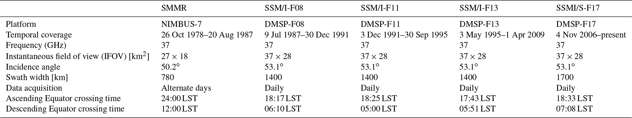
We use Ka band (37 GHz) horizontally polarized T_b data produced within the framework of a NASA MeASUREs project and distributed at the spatial resolution of 3.125 km (Brodzik et al., 2016) over the Northern Hemisphere. Specifically, we use data collected by the Scanning Multichannel Microwave Radiometer (SMMR), SMMR-Nimbus 7; the special sensor microwave/imager (SSM/I), SSM/I-F08, SSM/I-F11 and SSM/I-F13; and the special sensor microwave imager/sounder, SSMI/S-F17 (Table 1), because of its higher orbit stability (http://www.remss.com/support/crossing-times/, last access: 26 May 2021). Currently, the product time series begins in 1979 and ends in 2019. Data are provided twice a day, as morning and evening passes. Beginning and ending acquisition times for the morning and evening passes are contained within the product's metadata, along with other information. More information can be found at https://nsidc.org/data/nsidc-0630/versions/1 (last access: 26 May 2021).

Table 1 Characteristics of the PMW sensors used for this work. LST denotes local solar time.

Historical gridding techniques for PMW spaceborne datasets (Armstrong et al., 1994, updated yearly; Knowles et al., 2000, 2006) are relatively simplistic and were produced on grids (Brodzik and Knowles, 2002; Brodzik et al., 2012) that are not easily accommodated in modern software packages. Specifically, the coarse-resolution gridding methodology is based on a simple “drop-in-the-bucket” average, i.e., all of the measurements within a given time falling into a specific pixel are averaged. In the reconstruction algorithm used for the enhanced T_b, the so-called effective measurement response function, determined by the antenna gain pattern and being unique for each sensor and sensor channel, is used in conjunction with the scan geometry and the integration period. The gridding approach uses the Backus–Gilbert technique (Backus and Gilbert, 1967, 1968), a general method for inverting integral equations, which has been applied for solving sampled signal reconstruction problems (Caccin et al., 1992; Stogryn, 1978; Poe, 1990), for spatially interpolating and smoothing data to match the resolution between different channels (Robinson et al., 1992), and for improving the spatial resolution of surface T_b fields (Farrar and Smith, 1992; Long and Daum, 1998). An example of T_b maps at 37 GHz, horizontal polarization, in the case of both the coarse- and enhanced-resolution products over Greenland on 16 July 2001 is reported in Fig. 1. The higher detail captured by the enhanced spatial resolution is clearly visible, especially along the ice sheet edges, where melting generally occurs at the beginning of the season and lasts for the remaining part of the summer. Figure 2 shows an example of time series of both coarse and enhanced PMW T_b (again at 37 GHz, horizontal polarization) for the pixel containing the Swiss Camp station. From the figure, we observe that the two time series are highly consistent with each other, with a mean difference of 0.895 K and a standard deviation of 4.89 K, indicating that the potential noise introduced by the enhancement process is not a major issue. However, differences do exist, as in the case of 3 April 2012 (day of the year 93), when the enhanced product suggests the presence of melting while the coarse product does not. This is likely due to the different spatial resolutions between the two products, as we discuss in the following sections, and shows the added value of using the 37 GHz frequency in detecting small-scale features of the melting process.

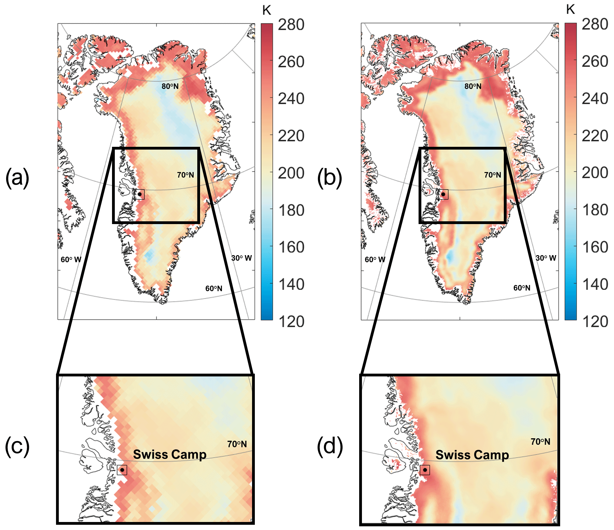
Figure 1 Maps of PMW T_b at 37 GHz, horizontal polarization, acquired over Greenland on 16 July 2001 with the (a) coarse (25 km) and (b) enhanced (3.125 km) resolution products. Panels (c) and (d) refer to the area highlighted in the square in panels (a) and (b).

To compare our results with precedent PMW surface melting products, we also perform our calculations with the commonly used PMW dataset by Mote (2014). The dataset consists of a daily melt maps product obtained from 37 GHz T_b from SMMR, SSM/I and SSMI/S available on a 25 km grid. This comparison enables us to see the advantages of using the enhanced-resolution product with respect to a coarser-resolution surface melt product. The dataset is generated using a dynamically changing threshold (Mote, 2007) obtained by simulating the T_b change for every grid cell, each year, using a microwave emission model (Mote, 2014). The dataset covers the temporal window from 1979 to 2012 and is available at the National Snow and Ice Data Center (NSIDC) website (https://nsidc.org/data/NSIDC-0533/versions/1, last access: 26 May 2021).

2.2 Greenland air temperature data

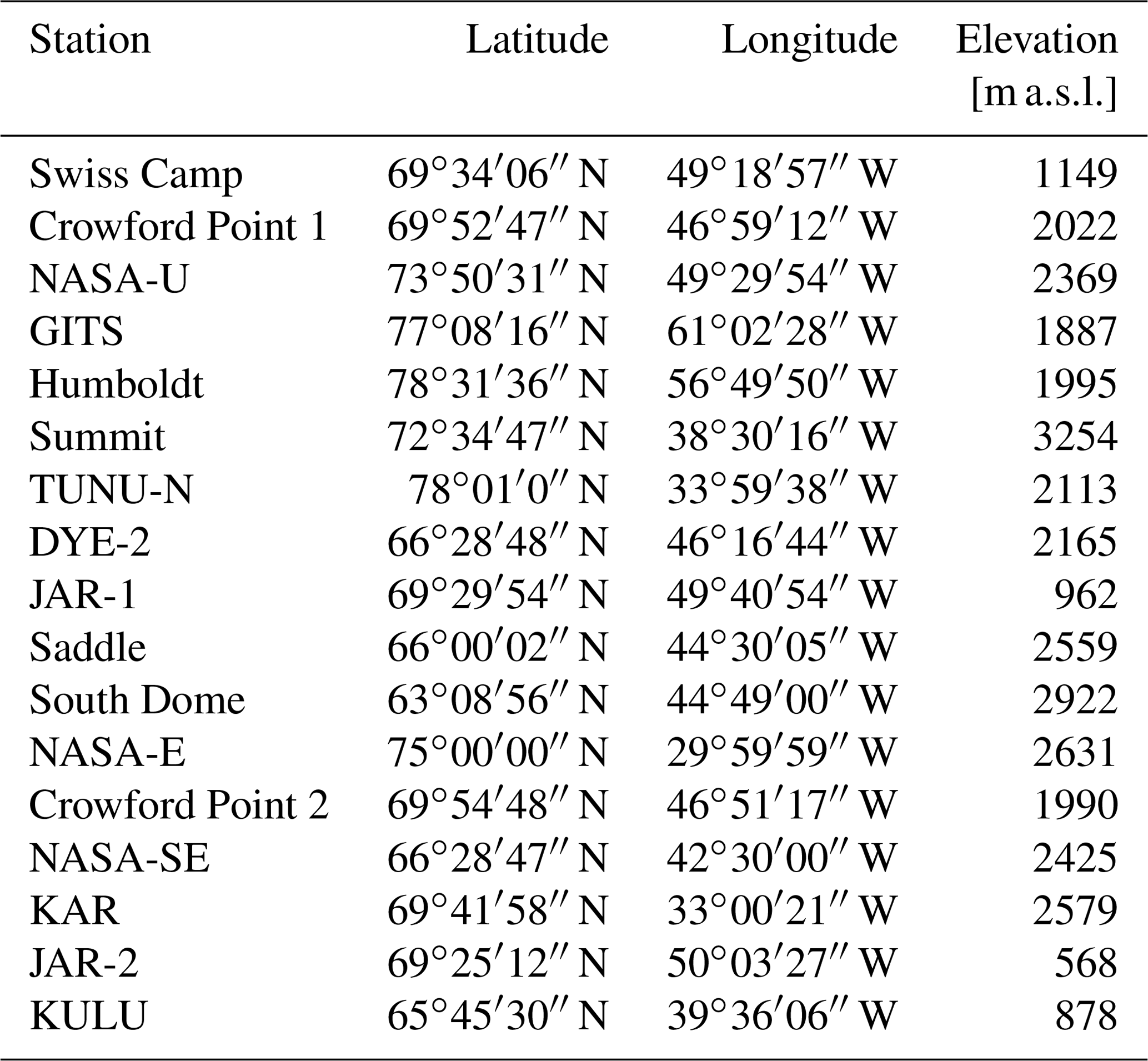
In order to assess the results obtained from PMW data, we use in situ data collected by AWSs distributed over the Greenland ice sheet. In the absence of direct observations of melting, we use air temperature (3 m above the surface) to extrapolate instances when liquid water is present, following the procedure adopted by Tedesco (2009) for Antarctica. Specifically, we use data recorded by stations of the Greenland Climate Network (GC-Net; Steffen et al., 1996). The AWSs provide continuous measurements of air temperature, wind speed, wind direction, humidity, pressure and other parameters. We focus on air temperature data collected every hour by the 17 selected stations reported in Table 2. We considered a validation period from 2000 (when all of the considered AWSs were in operation) to 2016 and used daily averaged values. More information about the GC-Net dataset can be found at http://cires1.colorado.edu/steffen/gcnet/ (last access: 26 May 2021).

Table 2 Locations of the automatic weather stations of the Greenland Climate Network (GC-Net) sites used to validate the results in this study.

2.3 The MAR model

We assess the enhanced PMW-based surface melt maps with the outputs of the Modèle Atmosphérique Régional (MAR, e.g., Alexander et al., 2014; Fettweis et al., 2013, 2017; Tedesco et al., 2013) regional climate model. MAR is a modular atmospheric model that uses the σ-vertical coordinate to simulate airflow over complex terrain and the soil ice snow vegetation atmosphere transfer scheme (e.g., De Ridder and Gallée, 1998) as the surface model. MAR outputs have been assessed over Greenland (e.g., Fettweis et al., 2005, 2017; Alexander et al., 2014). The snow model in MAR, which is based on the Crocus model of Brun et al. (1992), calculates albedo for snow and ice as a function of snow grain properties, which in turn depend on energy and mass fluxes within the snowpack. Lateral and lower boundary conditions of the atmosphere are prescribed from reanalysis datasets. Sea surface temperature and sea ice cover are prescribed using the same reanalysis data. The atmospheric model within MAR interacts dynamically with the surface model.

In this study, we use the output from MAR version v3.11.2, which is characterized by an enhanced computational efficiency and improved snow model parameters (Fettweis et al., 2017; Delhasse et al., 2020). The model is forced at the boundaries using ERA5 reanalysis (Hersbach et al., 2020), which is the newest generation of global atmospheric reanalysis data that superseded ERA-Interim (Dee et al., 2011), and output is produced at a horizontal spatial resolution of 6 km. In order to compare output from MAR with estimates of melt extent obtained from PMW data, we average the liquid water content (LWC) simulated by MAR along the first 5 cm and 1 m from the surface of the vertical profile of the snowpack, following Fettweis et al. (2007).

2.4 Melt detection algorithms

Generally speaking, melt detection algorithms can be divided into threshold-based and edge-detection algorithms (e.g., Liu et al., 2005; Joshi et al., 2001; Steiner and Tedesco, 2014). Here, we focus on threshold-based algorithms, detecting melting when T_b values (or their combination) exceed a defined threshold, which is computed in different ways depending on the algorithm. For example, Steffen et al. (1993) used the normalized gradient ratio GR $=(T_{\mathrm{b}\mathrm{19}\mathrm{H}}-T_{\mathrm{b}\mathrm{37}\mathrm{H}})/(T_{\mathrm{b}\mathrm{37}\mathrm{H}}+T_{\mathrm{b}\mathrm{19}\mathrm{H}})$ to detect wet pixels with a threshold value computed based on in situ measurements. This method was later updated by Abdalati and Steffen (1995) who introduced the cross-polarized gradient ratio XPGR $=(T_{\mathrm{b}\mathrm{19}\mathrm{H}}-T_{\mathrm{b}\mathrm{37}\mathrm{V}})/(T_{\mathrm{b}\mathrm{37}\mathrm{H}}+T_{\mathrm{b}\mathrm{19}\mathrm{V}})$, where the Ka-band component of the algorithm was switched from horizontally to vertically polarized.

Ashcraft and Long (2006) proposed a threshold based on dry (winter) and wet snow T_b as $T_{\mathrm{c}}=\mathit{\alpha }M+(\mathrm{1}-\mathit{\alpha })T_{\mathrm{wet}}$, where M is the average of winter T_b (January and February), T_wet is fixed as 273 K and T_c indicates the threshold value (we keep the same notation in the following). The mixing coefficient α=0.47 was derived considering LWC = 1 % in the first 4.7 cm of the snowpack. Similarly, a method based on a fixed threshold (set to 245 K and derived from the outputs of an electromagnetic model) above which melting is assumed to be occurring was proposed in Tedesco et al. (2007). Several other studies have detected melting when the T_b values exceed the mean winter value plus an additional value ΔT_b (M+ΔT_b approaches) associated with the insurgence of liquid water within the snowpack:

$$\begin{array}{}\text{(1)}& T_{\mathrm{c}}=M+\mathrm{\Delta }{T}_{\mathrm{b}}.\end{array}$$

Torinesi et al. (2003) proposed a value of ΔT_b=Nσ with M and σ (standard deviation of the time series) varying in space (specific pixel) and time (specific year) but a fixed value of N=3 from the analysis of weather station temperature data. Zwally and Fiegles (1994) used a fixed value of ΔT_b=30 K. Tedesco (2009) proposed an alternative approach based on the outputs of the Microwave Emission Model of Layered Snowpack (MEMLS) electromagnetic model (Wiesmann and Mätzler, 1999). In this case, an ensemble of outputs is generated by the MEMLS model by varying the inputs (e.g., correlation length, LWC and snow density). These outputs are then used to build a linear regression model for the ΔT_b that is a function of the winter T_b value as follows:

$$\begin{array}{}\text{(2)}& \mathrm{\Delta }{T}_b=\mathit{\phi }M+\mathit{\omega },\end{array}$$

with the values of the coefficients obtained from the linear regression. This is done to account for the increment related to the presence of LWC within the snowpack as a function of the snow properties: a fixed increase would correspond to different LWC values, potentially making the mapping of the wet snow areas inconsistent in terms of LWC values. For example, a snowpack with a small grain size would require a relatively larger amount of LWC compared with a snowpack with a larger grain size for the T_b values to increase by 30 K. From a complementary point of view, an increase of 30 K due to the presence of liquid water in the case of a snowpack with relatively coarse grains would correspond to a lower LWC value than an increase occurring in a snowpack with a smaller grain size. In summary, the adoption of this approach provides consistency in terms of the minimum LWC that is detected by the algorithm. Building on Tedesco (2009), we considered the LWC value of 0.2 %. The coefficients are $\mathit{\phi }=-\mathrm{0}$.52 and ω=128 K (R²=0.92). The T_b threshold value computed in this case can, therefore, be written as follows:

$$\begin{array}{}\text{(3)}& T_{\mathrm{c}}=M+\mathit{\phi }M+\mathit{\omega }=(\mathrm{1}+\mathit{\phi })M+\mathit{\omega }=\mathit{\gamma }M+\mathit{\omega },\end{array}$$

where γ and ω assume the values of 0.48 and 128 K, respectively.

Here, we focus five approaches: the M+ΔT_b approach with ΔT_b equal to 30 K and, to test the sensitivity to Zwally and Fiegles (1994), 35 and 40 K (M+30, M+35 and M+40 from here on); the algorithm based on MEMLS for LWC = 0.2 % (referred to simply as MEMLS from here on for brevity); and the 245 K fixed threshold (245 K from here on). We selected M+ΔT_b and MEMLS due to their higher accuracy in detecting both sporadic and persistent melting with respect to the other approaches presented above, i.e., Torinesi et al. (2003) and Ashcraft and Long (2006), as proven in previous studies (Tedesco, 2009). We also selected the 245 K approach to test a more conservative technique aimed at detecting persistent melting only. In the following sections, we report the results of two algorithms, namely the one using a fixed threshold of 245 K and the one based on MEMLS.

2.5 Inter-sensor calibration

In view of the novelty of this PMW dataset introduced by the enhancement in spatial resolution thanks to the improvement of the gridding technique, we first focus on the cross-calibration of the data acquired by the different sensors. This initial processing step aims to account for biases and differences associated with swath width, view angle, altitude and local time of day as well as the specific intrinsic differences associated with each sensor on the different platforms (Table 1). Several approaches have been proposed in the literature to address this issue for the historical, coarser-spatial-resolution gridded datasets (e.g. Cavalieri et al., 2012). For example, Jezek et al. (1993) compared SMMR and SSM/I over the Antarctic ice sheet for the K and Ka bands (∼ 19 and ∼ 37 GHz) for both horizontal and vertical polarizations. Steffen et al. (1993) proposed an approach that was focused over Greenland for the K band. Abdalati et al. (1995) derived relations between SSM/I observations for the SSM/I-F08 and SSM/I-F11 platforms over Antarctica and Greenland for 19.35, 22.2 and 37 GHz. Dai et al. (2015) intercalibrated SMMR, SSM/I (SSM/I-F08 and SSM/I-F13) and SSMI/S-F17 over snow-covered pixels in China and SMMR, SSM/I and AMSR-E (Advanced Microwave Scanning Radiometer on NASA's Earth Observing System) over the whole Earth surface sampling hot and cold pixels.

Given the novelty of the T_b products used here and the absence of the specific intercalibration of data collected from different platforms for this product, we developed an ad hoc intercalibration for the enhanced PMW dataset. Following Stroeve et al. (1998), we perform the intercalibration using only data collected over the Greenland ice sheet. We perform a linear regression between the data acquired by two sensors over the Greenland ice sheet and calculate the slope (m) and intercept (q) of the linear regression:

$$\begin{array}{}\text{(4)}& y=mx+q.\end{array}$$

In Eq. (4), x and y represent the T_b values from coincident data from the two overlapping satellite products. We consider two approaches to compute the m and q values in Eq. (4). In the first method, we compute the weighted average of the daily slope and intercept values from the regression of daily data. Considering n days, for every ith day we first compute m_i, q_i and the coefficient of determination for the linear regression of Eq. (4) ($R_i^{\mathrm{2}}$); we then average them according to Eqs. (5) and (6):

$$\begin{array}{}\text{(5)}& {\displaystyle }m={\displaystyle \frac{\sum _{i=\mathrm{1}}^n{m}_i{R}_i^{\mathrm{2}}}{\sum _{i=\mathrm{1}}^n{R}_i^{\mathrm{2}}}},\text{(6)}& {\displaystyle }q={\displaystyle \frac{\sum _{i=\mathrm{1}}^n{q}_i{R}_i^{\mathrm{2}}}{\sum _{i=\mathrm{1}}^n{R}_i^{\mathrm{2}}}}.\end{array}$$

This choice assigns higher values to the weights obtained from pairs of data with higher correlation. In the second method, we consider all values for all days when data from both platforms are available and then evaluate m and q using a linear regression fitting procedure based on least squares fitting. Using the estimated m and q values, we then correct the values for one of the sensors by applying Eq. (4) to the T_b values of one sensor (x, e.g., SMMR) to obtain new corrected T_b values (y).

We perform an additional comparison using the average difference between the T_b values and evaluating the match between histograms of the overlapping data (Dai et al., 2015) by means of the Nash–Sutcliffe efficiency (NSE) coefficient (Nash and Sutcliffe, 1970), defined as

$$\begin{array}{}\text{(7)}& \mathrm{NSE}=\mathrm{1}-{\displaystyle \frac{\sum {\left(h_i\left(T_{\mathrm{b}}^{\mathrm{A}}\right)-h_i\left(T_{\mathrm{b}}^{\mathrm{B}}\right)\right)}^{\mathrm{2}}}{\sum {\left(h_i\left(T_{\mathrm{b}}^{\mathrm{B}}\right)-\overline{h}\left(T_{\mathrm{b}}^{\mathrm{B}}\right)\right)}^{\mathrm{2}}}}.\end{array}$$

Here, h_i is the absolute frequency of the ith value of T_b of the two sensors (A and B) considered. The NSE is usually applied in calibration and validation procedures to assess the match between measured and modeled quantities, as in Sect. 4.2. After the application of linear relations found using Eqs. (4)–(6), in order to quantitatively assess the impacts of the intercalibration on T_b values, we computed the absolute difference between the values of the histograms of the T_b as follows:

$$\begin{array}{}\text{(8)}& D_i=\left|h_i\left(T_{\mathrm{b}}^{\mathrm{A}}\right)-h_i\left(T_{\mathrm{b}}^{\mathrm{B}}\right)\right|,\end{array}$$

where D_i is the absolute difference between the two histograms A and B for the ith value of T_b. We then summed the differences over the total number of pixels and computed the relative variation as follows:

$$\begin{array}{}\text{(9)}& d={\displaystyle \frac{D_{\mathrm{original}}-D_{\mathrm{corrected}}}{D_{\mathrm{original}}}},\end{array}$$

where D_original and D_corrected are the summations of D_i before and after the calibration, respectively. The relative variation in d can range from −∞, indicating a worse match of the histograms, to 1, indicating a perfect match of the histograms after the intercalibration.

2.6 Spatial autocorrelation: the variogram analysis

Variogram analysis is generally adopted in geostatistical analyses to evaluate the autocorrelation of spatial data (Delhomme, 1978; Edward et al., 1989) with variograms being characterized by three parameters: the sill, the range and the nugget effect. The sill is the variance value at which the variogram becomes flat. The range is the distance at which the variogram reaches the sill. Beyond this value, the data are no longer autocorrelated. The nugget effect is the variance value at null distance, theoretically zero and resulting from measurement errors or highly localized variability. We computed the empirical variogram as

$$\begin{array}{}\text{(10)}& \mathit{\gamma }\left(\mathit{\delta }\right)={\displaystyle \frac{\mathrm{1}}{\mathrm{2}N\left(\mathit{\delta }\right)}}\sum _{i,j\in N\left(\mathit{\delta }\right)}(x_i-x_j{)}^{\mathrm{2}},\end{array}$$

where γ is the semi-variance, N(δ) is the number of pair measurements (i,j) spaced by distance δ, and x_i and x_j are the respective values of the ith and jth measured variable. Generally, the semi-variance γ increases as the distance δ increases according to the principle that close events are more likely to be correlated than distant events. The experimental variogram is the graphical representation of the semi-variance γ as a function of the distance δ. Finally, the experimental variogram is fitted with a function (here, we use a spherical function) to compute the sill, the range and the nugget effect.

3 Results and discussion

3.1 Inter-sensor calibration of enhanced-resolution passive microwave data

First, we show the results obtained for the inter-sensor calibration of the selected satellite constellation. The overlapping periods for the different sensors are as follows: SMMR and SSM/I-F08 overlap between 9 July and 20 August 1987 for a total of 22 d (1 d every 2 d as sensed by the SMMR sensor); SSM/I-F08 and SSM/I-F11 overlap between 3 and 18 December 1991 for a total of 16 d; SSM/I-F11 and SSM/I-F13 overlap between 3 May and 30 September 1995 for a total of 76 d; and SSM/I-F13 and SSM/S-F17 overlap for the period from 1 March to 10 December 2008 for a total of 71 d. In Fig. 3, we show the scatterplots of the data used for the linear regression for Greenland for both evening and morning passes for the SMMR and SSM/I-F08 sensors, reporting m, q and R² values. We point out that the overlap between SMMR and SSM/I-F08 data occurs in the months of July and August. During these months, the differences between acquisition times (Table 2) might lead to biases and errors associated with snow conditions (e.g., wet vs. dry). Specifically, we expect larger errors at the beginning of the melting season when snow undergoes thawing–refreezing cycles during the day, with frozen snow (low T_b values) potentially being present early in the morning and late at night (SMMR ascending and SSM/I-F08 descending passes) and liquid water (high T_b values) being present during the day. In Table 3, we report the average values of the difference between pairs of T_b data and the NSE coefficient values for the histograms of the same pairs. In Table 4, we report the values for the slope and intercept obtained from the linear regression analysis of enhanced PMW T_b (37 GHz, horizontal polarization) over Greenland for SMMR vs. SSM/I-F08, SSM/I-F08 vs. SSM/I-F11, SSM/I-F11 vs. SSM/I-F13 and SSM/I-F13 vs. SSM/S-F17, along with the R² values and d values computed according to Eq. (6). In the case of SSM/I and SSMI/S, R² values are higher, mostly around 0.98. In Fig. 4, we also show examples of histograms for the SMMR and SSM/I-F08 sensors. Large differences are obtained for these sensors for both the evening and morning passes, likely because of the difference in overpass time and the presence or absence of melting in some of the scenes observed by one sensor but not present in the other (Table 3). Conversely, for the SSM/I and SSMI/S sensors, the average difference is close to 0 K (with the exception of the F-08 and F-11 satellites, which show an average difference slightly larger than 1 K, consistent with previous results obtained by Abdalati et al. (1995) in the case of the 25 km resolution data), and the NSE values are extremely close to 1 (Table 3). For of SMMR and SSM/I-F08, the higher average difference (ranging between −3.4 and −4.3 K) and the relatively lower NSE values (ranging between 0.89 and 0.96) show that these sensors have the largest bias. Lastly, we only applied the correction to SMMR, and we did not apply the linear regression to the SSM/I-F08–SSM/I-F11, SSM/I-F11–SSM/I-F13 and SSM/I-F13–SSMI/S-F17 datasets as, in this case, the linear correction worsened the agreement between the two sets of measurements. We applied the correction coefficients obtained with the second method according to the higher relative improvement for the evening pass.

Table 3 Average enhanced-resolution T_b differences at 37 GHz, horizontal polarization, for the different PMW sensors and NSE coefficients computed for the histograms of T_b.

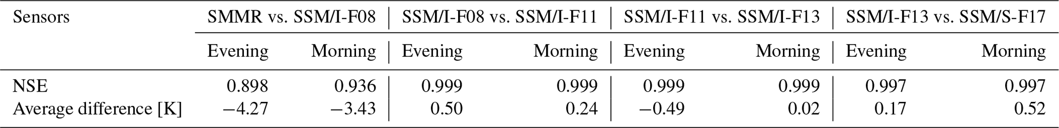
Table 4 Slope (m) and intercept (q) obtained from the linear regression analysis between the selected satellite pairs' enhanced PMW T_b at 37 GHz, horizontal polarization, over Greenland. The subscripts refer to the case where the coefficients are weighted by means of the R² (case 1, see Eqs. 5 and 6) or cases where they are not weighted by means of the R² (case 2). We also report the values for the R² and the d values computed according to Eq. (9).

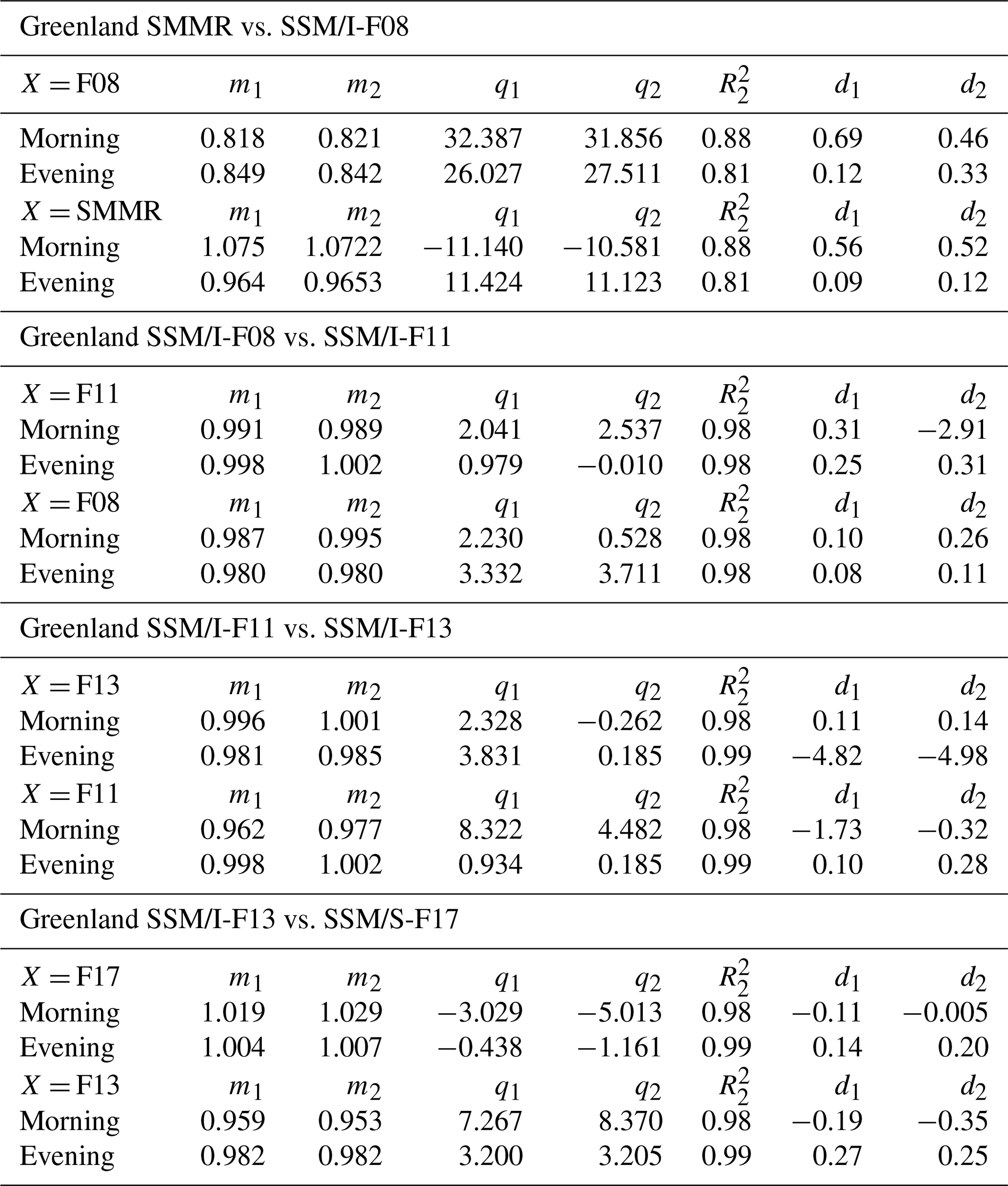
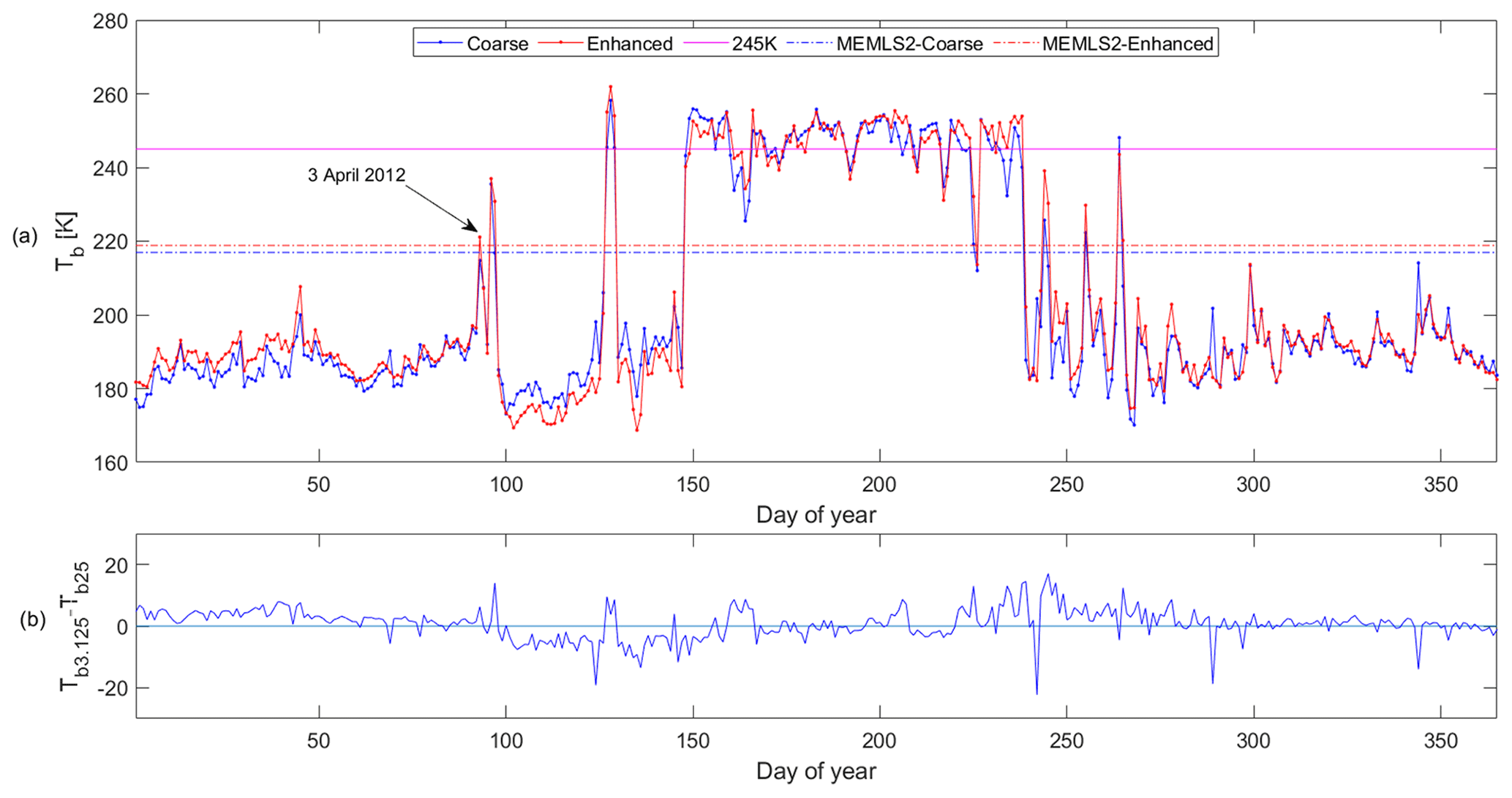
Figure 2 (a) Time series of T_b at 37 GHz, horizontal polarization, for the year 2012 for the pixel containing the Swiss Camp site in the case of the coarse (blue) and enhanced (red) products. Threshold values, shown as horizontal lines, are obtained from two approaches considered in this study: 245 K and MEMLS. (b) The difference between the 3.125 km and the 25 km T_b time series for the same pixel (mean of 0.895 K and standard deviation of 4.89 K).

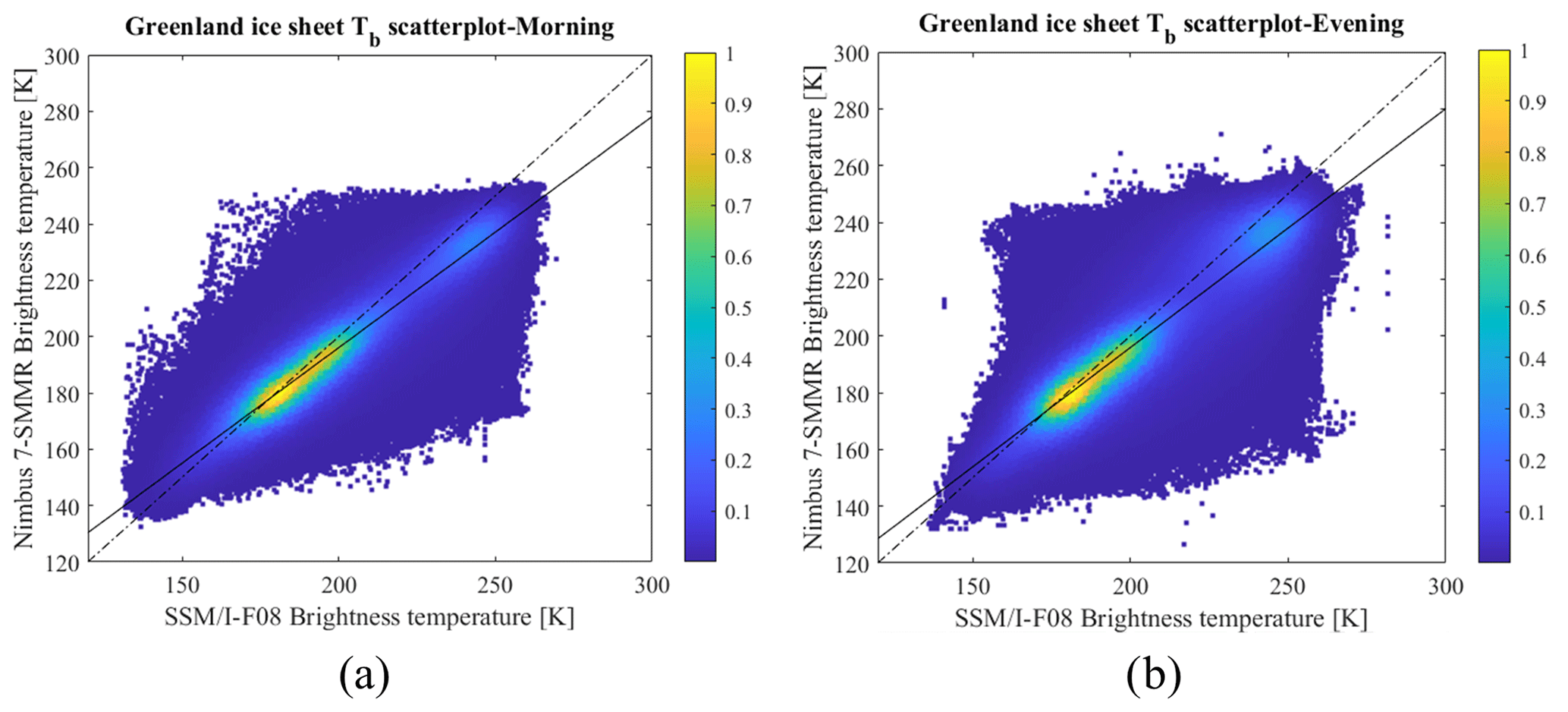
Figure 3 Density scatterplots of SMMR and SSM/I-F08 T_b data sensed during the overlap period (9 July–20 August 1987) of the two sensors over the Greenland ice sheet for (a) morning and (b) evening passes. The solid black lines show the linear fitting, and the dashed black lines show the 1:1 line. The color palette indicates the relative frequency.

Figure 4 Histograms of T_b before and after the application of the intercalibration relations (for Greenland). Relations are applied for both evening (a) and morning (b) passes, and the histograms of the data and the distance (absolute value of the difference as in Eq. 8) between the histograms for original data are reported. The left column represents the uncorrected data, the central column represents the results applying the correction to SMMR data and the right column represents the results applying the correction to the SSM/I data.

3.2 Assessment of melt detection algorithms

In order to assess the capability of the selected algorithms, we compare the outputs obtained by PMW data with in situ air temperature averaged daily from AWSs as an index of surface melting (Braithwaite and Oelsen, 1989) and with the liquid water content simulated by the MAR regional climate model. We first evaluate performance at the local scale (at the specific locations of the selected AWSs), comparing the number and the concomitance of melting days according to PMW data and the ground-truth reference. According to the results obtained, we then focus on the MEMLS and 245 K algorithms to evaluate the capability of the two approaches with respect to describing the surface melt extent at the ice sheet scale.

3.2.1 Assessment with AWS data

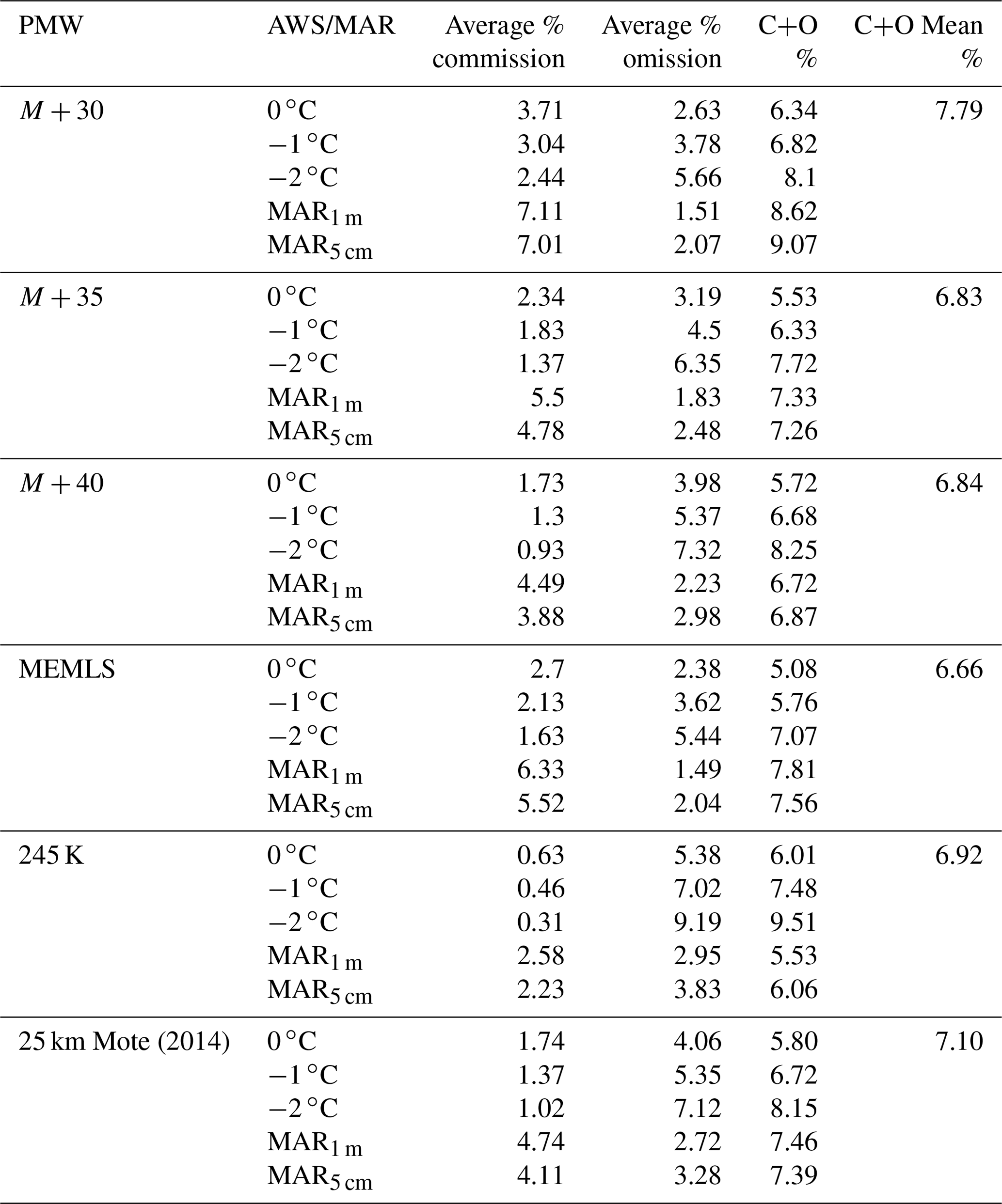
Historically, the presence of liquid water within the snowpack using data from AWS has been estimated when recorded air temperature exceeds a certain threshold during the day. Because melting can also occur due to radiative forcing (i.e., solar radiation) and the air temperature does not necessarily represent the snow surface temperature, we tested three threshold values for air temperature, 0, −1 and −2 ^∘C, as in Tedesco (2009). We assessed the performance of the PMW-based algorithm by defining commission and omission errors. Commission errors occur when melting is detected by PMW data but not by AWS data, and omission errors occur when melting is detected by AWS data but not by PMW data. The results of the error analysis are summarized in Table 5 for the different algorithms and for the Mote (2014) dataset for the different threshold values on the AWS air temperature values. In Table 5, commission and omission error values are reported as an average over all stations. Specific results for each AWS location are reported in the Supplement (Tables S2, S3 and S4) along with a map of the AWS network (Fig. S1). As a more general performance indicator, Table 5 also reports the sum of the two commission and omission errors, computed for each AWS case (C+O). Moreover, we show an average value of all of the C+O (for both AWS and MAR assessments, presented in the next subsection) for each PMW algorithm (C+O Mean) as a synthetic index of performance. Our results indicate that the 245 K algorithm shows the lowest commission error (between 0.31 % and 0.63 %) and the highest omission error (between 5.38 % and 9.19 %). This is consistent with this algorithm being the most conservative among those considered (i.e., the algorithm is not sensitive to sporadic melting). In contrast, a higher commission error is achieved for the M+30, M+35 and M+40 thresholds, particularly for the Humboldt and GITS stations (northwestern Greenland), where the commission error is up to 1 order of magnitude larger than the MEMLS and 245 K algorithms for every ground-truth reference (e.g., from 0.70 % for MEMLS and 0.09 % for 245 K to 5.63 % for M+30, for an air temperature of 0 ^∘C). Moreover, for the MEMLS algorithm, we note the lowest omission error for the Swiss Camp, JAR-1 and JAR-2 sites (6.9 % for MEMLS and 8.4 % for M+30, 10.0 % for M+35, 12.4 % for M+40 and 17.4 % for 245 K). The coarse-resolution dataset presents a commission error of between 1.02 % and 1.74 % and an omission error of between 4.06 % and 7.12 %, confirming the capability of historical data to detect surface melting over the Greenland ice sheet. However, the enhanced-resolution dataset presents better results in terms of C+O when applying the M+40 and MEMLS algorithms. The sensitivity to the air temperature threshold is low, with commission and omission error decreasing by about 1 % and increasing by 3 %, respectively, when considering threshold values from 0 to −2 ^∘C.

Table 5 Performance of the PMW melt detection algorithms studied with AWS and MAR data. Five thresholds are used to detect melt at a 3.125 km resolution, and the Mote (2014) melting dataset is used as a 25 km resolution comparison. For each case, three thresholds (0, −1 and 2 ^∘C) are applied to the AWS data and two approaches (MAR_1 m and MAR_5 cm) are applied to the MAR-simulated LWC to detect melt. The performance of the respective PMW melting products is computed in terms of commission and omission errors averaged for all of the AWS sites considered. C+O refers to the total error considering both commission and omission. The average of the C+O of each melting dataset (C+O Mean) is reported as a synthetic index of performance.

In order to better understand the sources of the relatively high values of the commission errors at some locations, we show the time series of air temperature and T_b at 37 GHz, horizontal polarization, at three selected stations – (a) Summit, (b) Humboldt and (c) Swiss Camp – for the year 2005 (Fig. 5). The threshold values obtained with the different detection algorithms are also plotted as horizontal lines (black) along with the 0 ^∘C air temperature threshold (magenta). We selected these three locations as they are representative of three different environmental and melting conditions. The time series recorded at Summit station (Fig. 5a) shows the sensitivity of T_b to physical temperature and its seasonal variations. In this case, the air temperature remains below 0 ^∘C throughout year and the T_b signal does not exceed any threshold value (horizontal lines). This time series is typical of a location where melting is generally absent. The T_b time series collected for the Humboldt location (Fig. 5b) shows a strong and sudden peak starting on 20 July, when the air temperature average is about −0.5 ^∘C (detected by −1 and −2 ^∘C air temperature thresholds). This event is detected by all algorithms. Nevertheless, M+30 (and similar algorithms) also indicates the potential presence of melting for the period preceding the July melting (between 17 June and 17 July). This melting is not confirmed by the other algorithms or by the AWS analysis, suggesting that the threshold value used for these algorithms might be too low. Lastly, melting clearly occurs for the Swiss Camp site (Fig. 5c), which is characterized by a sharp and substantial increase in T_b beginning around mid-May. For this case, all algorithms detect melting, with MEMLS providing the lowest threshold and the 245 K fixed threshold being the most conservative. The computed rough estimation of the average emissivity for the period from 17 June to 17 July (T_b divided by the recorded air temperature) also suggests that melting is not occurring in the period considered for the Humboldt case, presenting an average emissivity that is even lower than in the Summit case. Figure 6 shows maps of surface melt extent obtained using the different approaches for 13 July 2008. Consistent with the results discussed above, the M+30 and M+35 algorithms suggest melting up to high elevations, within the dry snow zone, where it likely did not occur. The M+40 and MEMLS algorithms show similar results, whereas the 245 K fixed-threshold approach shows the most conservative estimates, as expected. As mentioned, the threshold algorithms for ΔT_b (M+30 etc.) rely on a fixed ΔT_b value, which could produce errors if a large seasonal range in T_b existed due to temperature variability. In contrast, the MEMLS algorithm is based on the linear regression of the ΔT_b as function of different combinations of dry snow conditions (LWC =0, i.e., different winter T_b means). This provides an appropriate threshold value that considers the snow conditions before melting and, at the same time, follows a more consistent approach with respect to the amount of LWC detected in the snowpack.

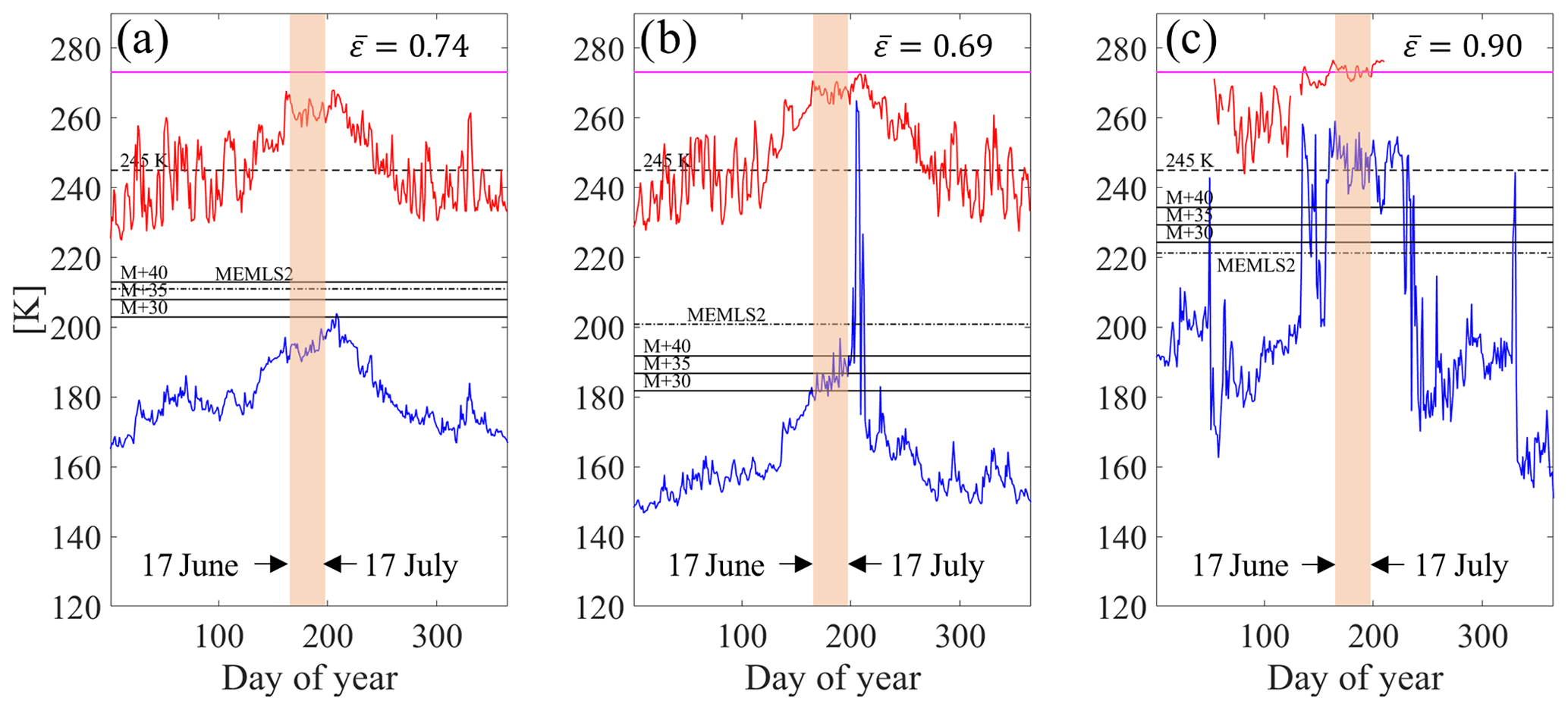
Figure 5 Time series of (blue) enhanced-resolution T_b 37 GHz, horizontal polarization, and (red) air temperature at the (a) Summit, (b) Humboldt and (c) Swiss Camp stations for the year 2005. Threshold values obtained with the different detection algorithms are reported as horizontal black lines (solid line, M+ΔT; dashed line, 245 K; and dot-dashed line, MEMLS), and the 0 ^∘C threshold is reported as a magenta solid line. The 30 d window between 17 June and 17 July is shown in the shaded orange area and reports the average estimated emissivity (ε) values.

3.2.2 Assessment with MAR outputs

For the comparison between PMW-based and MAR outputs, we averaged the vertical profiles of LWC computed by MAR to the top 5 cm (MAR_5 cm) and the top 1 m (MAR_1 m) of the snowpack following Fettweis et al. (2007). In order to be consistent with the minimum LWC to which the MEMLS algorithm is sensitive, we set the threshold on the LWC values at which we assume melting is occurring to 0.2 % for both depths. We selected two different depths for our analysis so that we could study two types of melting events: (1) sporadic surface melting, affecting the first few centimeters of the snowpack, and (2) persistent subsurface melting, affecting the snowpack from the surface up to around the first meter. For consistency with the AWS analysis, we report the results averaged over those MAR pixels containing the AWS stations discussed in the section above in Table 5. The comparison between the results obtained from the PMW and modeled LWC indicates that the more conservative approaches (i.e., 245 K) perform better when considering the case of MAR_5 cm. In fact, the 245 K threshold shows the lowest overall error for this case (C+O = 6.06 %). The coarse-resolution dataset shows a C+O error equal to 7.39 %, which is slightly lower than for MEMLS (7.56 %). For the top 1 m, all of the algorithms present similar performance on average, with the best performance again obtained for 245 K (C+O = 5.53 %). However, all of the M+ΔT_b algorithms present the same issue of larger commission errors compared with MEMLS and 245 K (e.g., from 0.99 % for MEMLS and 0.26 % for 245 K to 4.62 % for M+30) in northeastern Greenland (e.g., Humboldt and GITS stations, see Tables S2 and S3 in the Supplement). This confirms the results that we obtained from the comparison with AWS data, pointing out the overestimation of melting in some dry areas by M+ΔT_b. For both the MAR_1 m and MAR_5 cm cases, for all of the algorithms considered, we find a high commission error for the JAR-1, JAR-2 and Swiss Camp sites (between 10 % and 22 %).

In order to better understand the origins of these errors, we show further insights into the differences between the PMW T_b and MAR outputs in Fig. 7. Figure 7a and b show the time series of LWC averaged over the first 5 cm (MAR_5 cm) and 1 m (MAR_1 m) obtained from MAR at the Swiss Camp site, respectively. In Fig. 7c, we report the T_b time series and the daily average air temperature (threshold values reported as horizontal lines). We first note an early melt event (labeled LWC = 0.046 % in Fig. 7b for the 108th day of the year) detected by the PMW MEMLS algorithm and at the AWS station but apparently undetected in MAR_1 m. A closer look at the time series shows that MAR_1 m does in fact estimate a LWC of 0.046 % on this day, whereas MAR_5 cm estimates a LWC of 0.6 %. This suggests that in some cases (before the main melt season) the MEMLS algorithm is actually sensitive to the LWC in the first 5 cm of the snowpack, as a consequence of the approximation of the electromagnetic outputs imposed by the linear fitting. We also note a melt event (labeled as LWC = 0.5 % in Fig. 7b) at the end of the melting season detected by both AWS data (air temperature larger than −1 ^∘C) and MAR (both in the first 5 cm and 1 m of snow) but not by any PMW algorithm. The T_b time series reveals a small peak, but the signal is not strong enough to exceed any threshold. This corresponds to a rainfall event (simulated by MAR), suggesting that the sensitivity of the 37 GHz channel to liquid clouds could mask some melt events. Moreover, the T_b appears to be slightly lower than January–February average at the end of the melting season, possibly due to an increase in grain size after refreezing, leading to a lower emissivity.

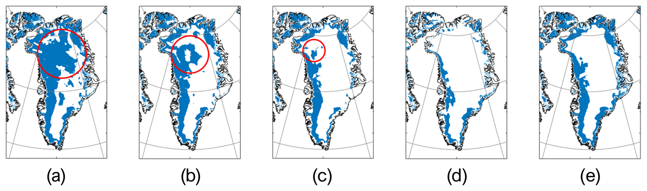
Figure 6 Melting maps obtained using the (a) M+30, (b) M+35, (c) M+40, (d) 245 K and (e) MEMLS algorithms over the Greenland ice sheet on 13 July 2008. An example of an area presenting the false detection problem is shown in the red circle.

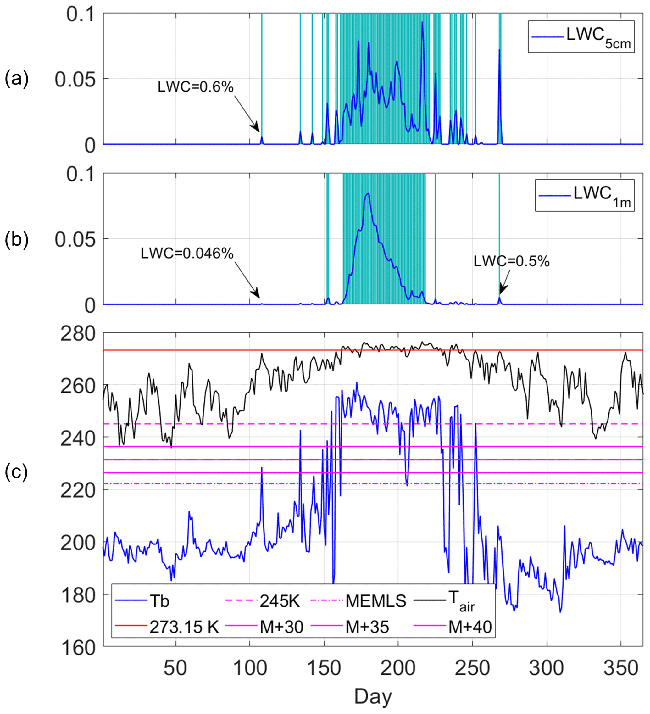
Figure 7 LWC from MAR averaged in the first 5 cm (a) and the first 1 m (b) of the snowpack. (c) Time series of the 37 GHz horizontally polarized T_b (3.125 km, blue), air temperature from AWS (black) and 245 K (dashed magenta line), M+ΔT (solid magenta lines) and MEMLS (dot-dashed magenta line) thresholds for the Swiss Camp site in the year 2001. Melting days according to MAR are marked as vertical light blue lines in panels (a) and (b).

The results discussed above (and the results from the comparison with AWS data) suggest that 245 K is the most conservative among the approaches tested in this study, providing the lowest (highest) commission (omission) errors, although being unable to detect sporadic melt events. On the contrary, the MEMLS and M+ΔT_b algorithms can detect sporadic melt events and present lower omission error compared with 245 K. However, the M+ΔT_b algorithms overestimate melting in some dry areas (the northwest of the ice sheet), suggesting melting when it is not actually occurring. On the contrary, the MEMLS algorithm is not affected by the large commission error in dry areas, presents the lowest omission error in the Swiss Camp area (along with M+30) and is still sensitive to low LWC levels. Considering the average error (C+O Mean in Table 5), the MEMLS algorithm shows the best performance (6.66 %). In view of the analysis presented and the different sensitivity to surface and subsurface melting, in the following we focus on the 245 K and MEMLS algorithms to study the extent of persistent and sporadic surface melting, respectively.

As a further analysis, we compared the PMW-retrieved melt extent with that estimated from MAR outputs. In Fig. 8 we show the time series of the melt extent integrated over the whole ice sheet for 2 selected years – (a) 1983 and (b) 2005, selected randomly to present an example of SMMR and SSM/I cases – estimated according to MAR_5 cm and MAR_1 m as well as the time series of the melt extent from the PMW data. The analogous figure for the coarse-resolution dataset is reported in the Supplement (Fig. S2). For each year, we compute the daily melt extent for the period from 1 May to 15 September and use the Nash–Sutcliffe efficiency (NSE) coefficient (Nash and Sutcliffe, 1970), described in Sect. 3, for a quantitative analysis. Here, we remind the reader that the NSE coefficient can assume values in the ($-\mathrm{\infty },\mathrm{1}$] interval. A perfect match between the two time series is achieved when the NSE coefficient is 1. NSE coefficient values in the [0,1] interval indicate that the modeled variable is a better predictor of the measurements than the mean. If the NSE coefficient is a negative number, the mean of the measured data describes the time series better than the modeled predictor. Here, we chose NSE = 0.4 as the efficiency threshold, considering that we compute melt extent at a daily timescale and from datasets at two different resolutions (i.e., resulting in an intrinsic bias related to the different pixel size). We compared the time series of the melt extent obtained using the 245 K algorithm with MAR_1 m (245 K vs. MAR_1 m) and the MEMLS melt extent with MAR_5 cm (MEMLS vs. MAR_5 cm) due to the expected differences in the sensitivity to detect persistent and sporadic melting between 245 K and MEMLS, respectively. We compare the melt extent obtained from the coarse-resolution dataset with MAR_5 cm, according to the similarity with MEMLS in terms commission and omission error. We report NSE coefficients computed for the 41-year (34-year for the coarse-resolution dataset) period in Table 6. At first, we notice that the comparison between 245 K and MAR_1 m produces large negative NSE coefficients for the 1979–1992 period, indicating an unsatisfactory match between PMW- and MAR-derived melt extents. The comparison between MEMLS and MAR_5 cm also presents negative NSE coefficient values (unsatisfactory results). Similarly, the coarse-resolution dataset shows negative NSE coefficient values, larger than MEMLS but smaller than 245 K. Between 1987 and 1992, we found larger but still negative NSE coefficients presenting smaller absolute values. Between 1993 and 2019, we found negative NSE coefficient values for 245 K and positive values for MEMLS for every year, indicating satisfactory results only for the latter algorithm. However, the coarse-resolution dataset only presents positive (but not satisfactory) NSE coefficient values in 2003 and 2012 (0.111 and 0.208, respectively). The time series in Fig. 8a reveals a strong underestimation of the 245 K-derived melt extent relative to MAR_1 m (the cause of the low NSE value, NSE $=-\mathrm{151}$.596) and shows a slightly better match for MEMLS (NSE $=-\mathrm{0}$.540). This result suggests that, for SMMR data, T_b values cannot always reach the 245 K threshold, even if the snowpack is saturated with liquid water and surface melting is developed, possibly due to a persistent bias after the intercalibration of the dataset. As a consequence, the 245 K threshold might be too high in the first part of the dataset, resulting in an underestimation of the melt extent. On the contrary, the MEMLS threshold, which is generally lower, can better capture the spatiotemporal evolution of surface melting, even if the melt extent is still underestimated. A possible consequence of the melt extent being underestimated in the first part of the time series is a slightly overestimated long-term trend. To address this possible implication, we compute long-term trends considering both the 1979–2019 and 1987–2019 reference periods in the next section. In Fig. 8b, the time series obtained with 245 K appears to better follow the temporal variability of the melt extent from MAR during the melting season, although it still presents a strong underestimation (NSE $=-\mathrm{5}$.250). On the other hand, the MEMLS-derived time series better matches the MAR-derived time series, showing a largely satisfactory NSE coefficient (0.782). In these 2 years the NSE coefficient computed for the coarse-resolution case is negative. The magnitude of the errors is lower than for the 245 K algorithm, indicating a weaker underestimation of the melt extent. This can be a consequence of the coarser resolution, which causes issues with respect to capturing melting areas at the edges of the Greenland ice sheet.

Table 6 Nash–Sutcliffe efficiency (NSE) coefficients computed for the comparison of the retrieved melt extent using the 245 K and MEMLS algorithms applied to the enhanced-resolution PMW T_b and MAR liquid water content outputs averaged in the first 1 m and the first 5 cm of the snowpack. The Nash–Sutcliffe efficiency coefficients for the comparison of the coarse-resolution dataset (Mote, 2014) are computed considering MAR_5 cm.

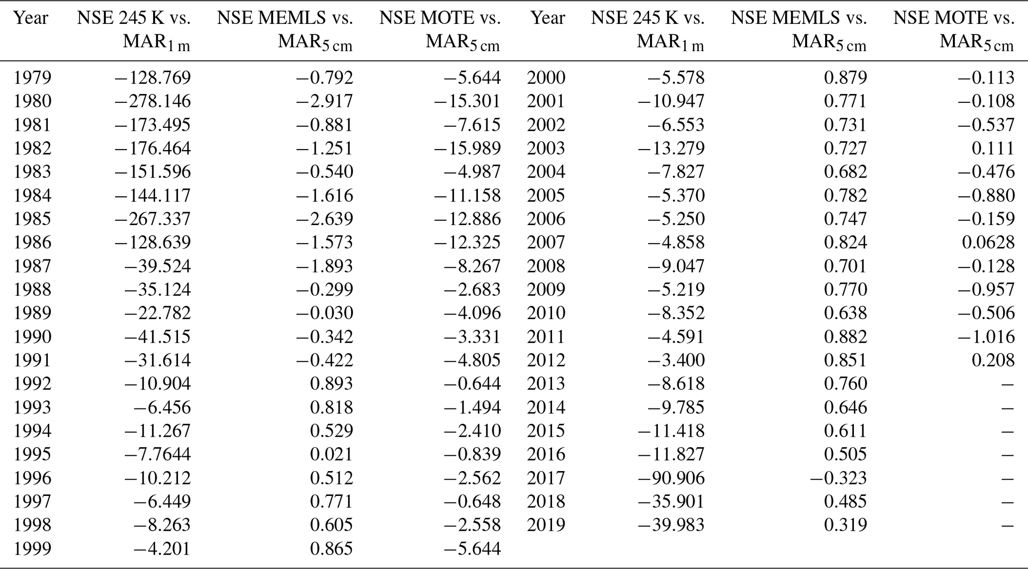
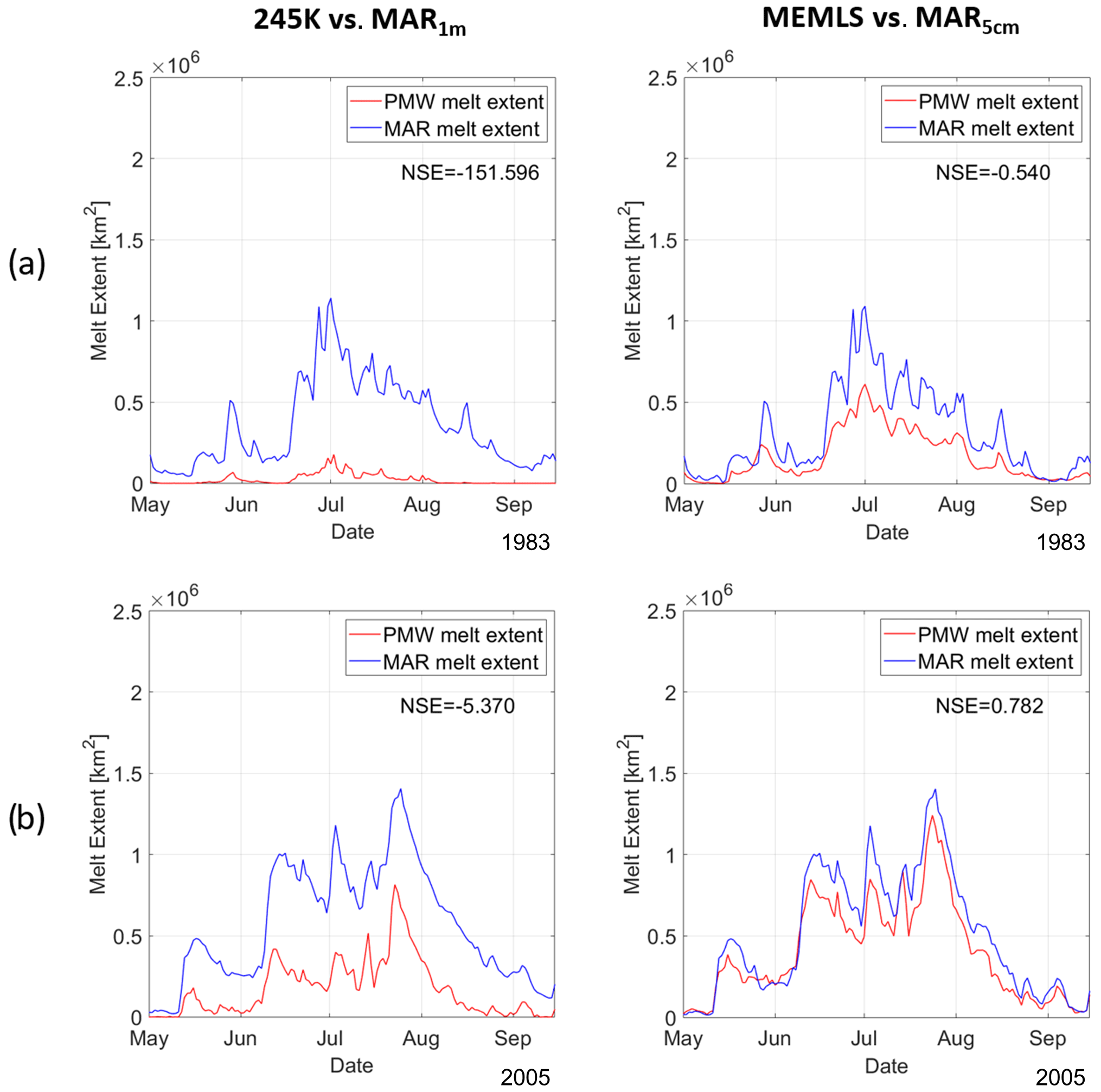
Figure 8 Melt extent estimation from PMW 37 GHz horizontally polarized T_b (red) and the MAR (blue) regional climate model. Time series were obtained using the 245 K algorithm and the LWC average in the first 1 m of the snowpack (left), and the MEMLS algorithm and the LWC average in the first 5 cm of the snowpack (right), for the years (a) 1983 and (b) 2005.

In summary, the 245 K threshold (even if presenting acceptable results in terms of commission and omission error considering both the AWS and MAR comparison) is too high to fully capture the melt extent everywhere over the ice sheet. Contrarily, we found that the MEMLS algorithm is suitable for capturing the evolution of melting over the Greenland ice sheet. The comparison with the 25 km historical surface melting dataset shows the same underestimation issue for 245 K. Although the 245 K case showed lower errors, we did not find acceptable NSE coefficient values.

3.3 Surface melting trends

Here, we report results concerning the trends in the melt duration, length of the melting season and melt extent. We define melt duration (MD) as the total number of days on which melting is detected. We compute trends in the MD over the whole ice sheet (mean melt duration, MMD, averaged over the total ice sheet area) and at a pixel-by-pixel scale. We also study the maximum melting surface (MMS, maximum extent of melting area, i.e., the sum of the pixel areas in which melting has been detected at least once over a period, expressed as a fraction of the total ice sheet area) and the cumulative melting surface or melting index (MI, the sum of the melting pixel days multiplied by the area subjected to melting, i.e., the integral of the MD time series; Tedesco et al., 2007). Lastly, we define melt onset date (MOD) and melt end date (MED) as the first day when melting occurs for 2 d in a row and when melting does not occur for at least 2 d in a row. We report the comparison with the trends computed according to the coarse-resolution dataset with reference to the time period of data availability (1979–2012). Figures related to this analysis can be found in the Supplement. In Fig. 9, we report the time series of the annual MMD, MMS and MI values for the 1979–2019 and 1988–2019 reference periods. We decided to look at two different reference periods in view of the fact that SMMR data are collected every other day and that the SMMR and SSM/I sensors are fundamentally different from one another (although this is not true for the remaining SSM/I sensors). We show the results obtained by applying the MEMLS algorithm (the one that presented the best performance in all of the cases considered) and the 245 K threshold (because it presents good performance in the omission and commission error analysis, even if it has the limitation of strongly underestimating the melt extent from the comparison with MAR outputs). For the MMD (Fig. 9a), we obtain a positive statistically significant (p value <0.05) trend from both the 245 K and MEMLS algorithms (except for the 1988–2019 period for 245 K): 0.249 d yr⁻¹ (0.108 d yr⁻¹) for the 245 K algorithm for the 1980–2019 (1988–2019) period and 0.451 d yr⁻¹ (0.291 d yr⁻¹) for the MEMLS algorithm. The trends computed using the coarse-resolution dataset results (Fig. S3a in the Supplement) equal 0.587 d yr⁻¹ for the 1979–2012 period and 0.595 d yr⁻¹ for the 1988–2012 period, which are smaller than MEMLS (0.704 and 0.671 d yr⁻¹, respectively) but larger than 245 K (0.457 and 0.418 d yr⁻¹, respectively). For the MMS (Fig. 9b), both the 245 K and MEMLS algorithms also indicate statistically significant positive trends (p value < 0.05 for every case and p value < 0.1 for MEMLS for the 1988–2019 period). The computed trends suggest that the MMS increased by 0.69 % yr⁻¹ in the case of MEMLS and by 0.94 % yr⁻¹ in the case of the 245 K algorithm for the 1979–2019 period (percentage with respect to the whole ice sheet surface area). For the 1988–2019 period, we also found that the trends are statistically significant but smaller in value (0.36 % yr⁻¹ for MEMLS and 0.47 % yr⁻¹ for 245 K). The obtained trends computed using the 25 km dataset (Fig. S3c in the Supplement) are equal to 1.31 % yr⁻¹ for the 1979–2012 period and 0.91 % yr⁻¹ for the 1988–2012 period, which are larger than the trends computed for MEMLS (1.03 % yr⁻¹ and 0.77 % yr⁻¹) but smaller than those computed for 245 K (1.50 % yr⁻¹ and 1.23 % yr⁻¹). In the case of MI (Fig. 9c), we also found positive statistically significant trends of 9.166 × 10⁵ km² d yr⁻¹ (MEMLS) and 5.862 × 10⁵ km² d yr⁻¹ (245 K) for the complete time series. When considering the reduced reference period, we found a 95 % statistically significant trend of 5.726 × 10⁵ km² d yr⁻¹ only in the case of MEMLS. The trends computed for the 25 km resolution dataset results (Fig. S3b in the Supplement) equal 0.999 × 10⁶ km² d yr⁻¹ (1979–2012) and 1.019 × 10⁶ km² d yr⁻¹ (1988–2012), which are smaller than those for MEMLS (1.428 × 10⁶ and 1.325 × 10⁶ km² d yr⁻¹, respectively) and 245 K for the 1979–2012 period (0.999 × 10⁶ km² d yr⁻¹) but larger than 245 K for the 1988–2012 period (1.019 × 10⁶ km² d yr⁻¹). Lastly, in Fig. 9d, we report the MOD and MED averaged spatially over the pixels with 95 % significant trends. We found that the average MOD (crosses in Fig. 9d) presents similar trends for 245 K and MEMLS considering both the entire and shortened time series: −0.546 and −0.273 d yr⁻¹ for 245 K, respectively, and −0.404 and −0.254 d yr⁻¹ for MEMLS, respectively. For the 1979–2012 (1988–2012) reference period, the trend in the MOD computed from the 25 km resolution dataset (Fig. S4a in the Supplement) was equal to −0.585 d yr⁻¹ (−0.562 d yr⁻¹), which is equal to and larger in absolute value than MEMLS between 1979 and 2012 (−0.585 d yr⁻¹) and MEMLS between 1988 and 2012 (−0.494 d yr⁻¹), respectively, but smaller than 245 K between 1979 and 2012 (−0.801 d yr⁻¹) and 245 K between 1988 and 2012 (−0.568 d yr⁻¹). On the contrary, we found larger differences when considering the reduced time series for the average MED (in red, Fig. 9), with results equal to 0.687 d yr⁻¹ for 245 K (1979–2019), 0.708 d yr⁻¹ for MEMLS (1979–2019) and 0.396 d yr⁻¹ for MEMLS (1988–2019). The 245 K algorithm does not present a statistically significant trend over the 1988–2019 period. This difference suggests that the 245 K algorithm may have stronger limitations with respect to capturing the last portion of the melting season for SMMR data, thereby confirming the problems observed with melt detection using this source of data vs. MAR_1 m simulations. The trends computed from the coarse-resolution dataset (Fig. S4b in the Supplement) are equal to 0.850 for the 1979–2012 period and 0.716 for the 1988–2012 period. For the 1979–2012 (1988–2012) period, we found a delay of 0.937 d yr⁻¹ (0.621 d yr⁻¹) for MEMLS and 1.046 d yr⁻¹ (0.521 d yr⁻¹) for 245 K.

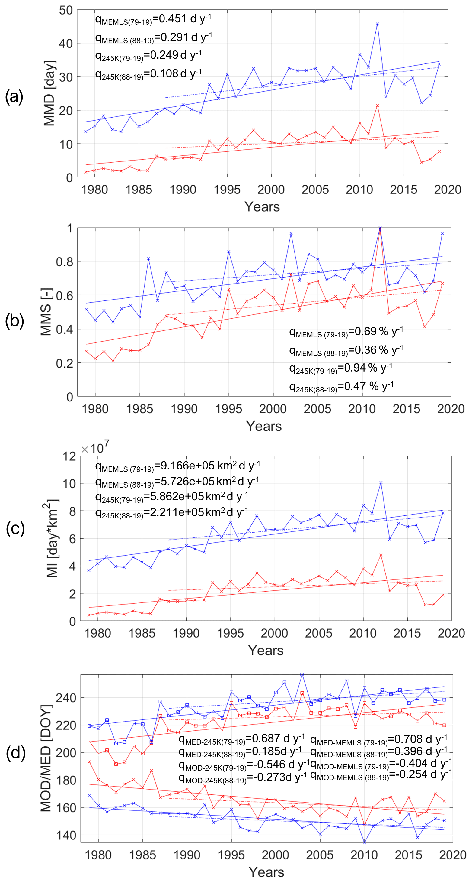
Figure 9 Time series of annual (a) mean melt duration (MMD), (b) maximum melting surface fraction (MMS, expressed as fraction of the surface area of the ice sheet), (c) melt index (MI), and (d) melt onset date (MOD) and melt end date (MED). Regression lines were computed for the 1979–2019 (solid line) and 1988–2019 (dot-dashed line) periods. The MMD is averaged over all of the Greenland ice sheet pixels. Red (blue) lines refer to the 245 K (MEMLS) algorithm; in panel (d), squares (crosses) refer to MED (MOD).

In Fig. 10 we show the trends in the MD, MOD and MED on a pixel-by-pixel basis for the complete time series (1979–2019). We found that the trend in the MD exhibits the highest statistical significance (in terms of the number of statistically significant pixels), being the most stable and reliable trend among the pixel-by-pixel parameters analyzed. We found mostly positive trends in the MD in all pixels (Fig. 10a, b), with higher values moving towards the coastline, maxima in the ablation zone of the Jakobshavn Glacier (2.40 d yr⁻¹ for 245 K and 2.66 d yr⁻¹ for MEMLS) and minima in high-altitude areas. We averaged the statistically significant trends, finding an average of 0.468 d yr⁻¹ for the 245 K algorithm and an average of 0.697 d yr⁻¹ for MEMLS. For MOD and MED, we found a lower number of statistically significant pixels. The statistically significant pixels exhibit a negative trend for MOD (Fig. 10c, d) and a positive trend for MED (Fig. 10e, f), with the melting season starting on average 0.694 d yr⁻¹ earlier and ending 0.680 d yr⁻¹ later according to the 245 K algorithm (0.360 d yr⁻¹ earlier and 0.909 d yr⁻¹ later for MEMLS). We point out that the average of the statistically significant trends is generally higher than the trends computed at the ice sheet scale as we computed the average over the statistically significant pixels only.

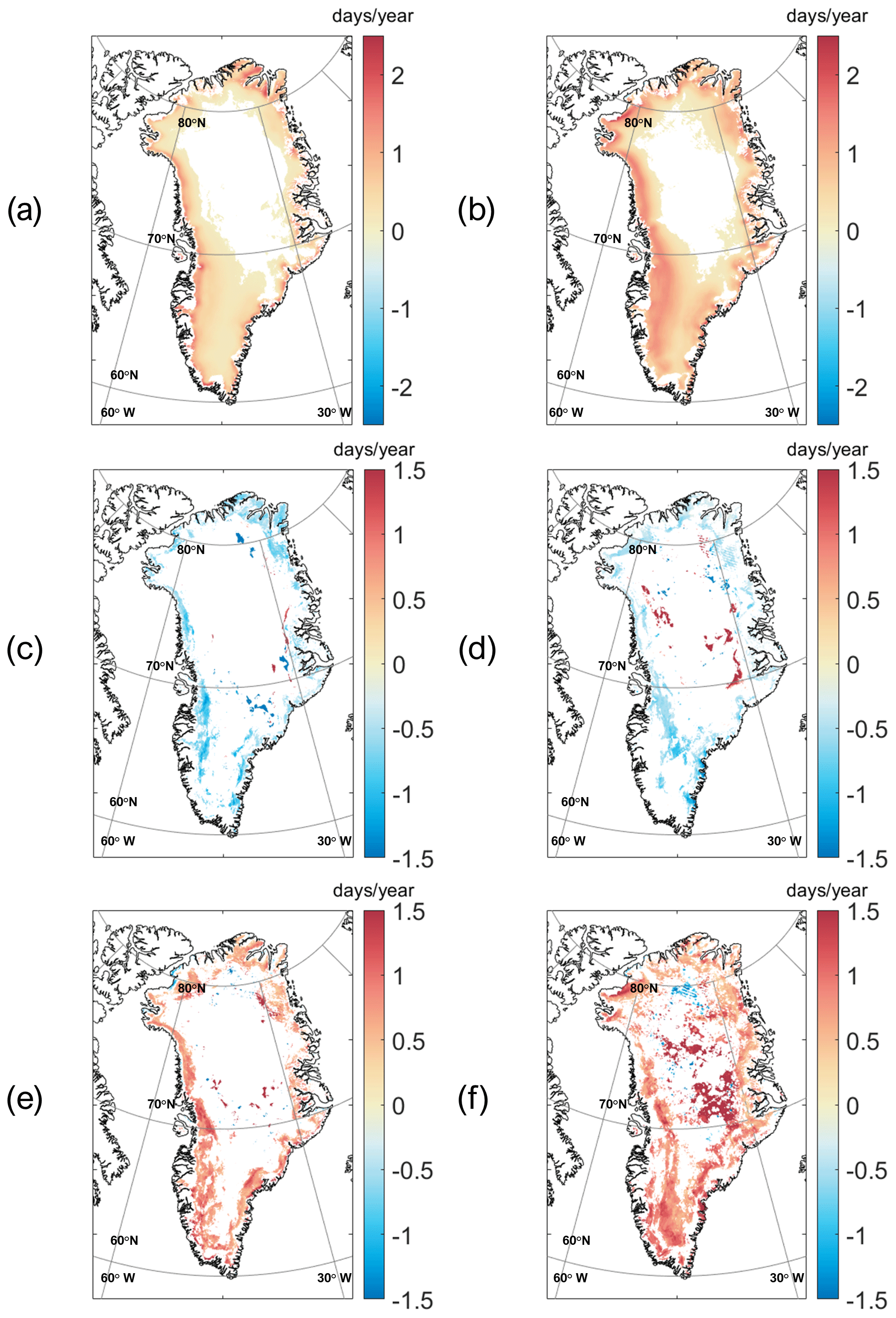
Figure 10 Maps of 95 % significant trends (1979–2019) obtained with the 245 K (a, c, e) and MEMLS (b, d, f) algorithms for melt duration (MD; panels a and b), melt onset date (MOD; panels c and d) and melt end date (MED; panels e and f). MOD and MED are defined as the first and last 2 melting days in a row.

3.4 Spatial information content

In order to investigate the spatial information content of the enhanced-resolution PMW data with respect to the coarser-resolution dataset, we also performed a variogram-based analysis of the MD estimated from the two products when using either the 245 K or the MEMLS algorithms. We point out that knowledge of scales is imperative for improving our understanding of the observed changes because processes and related relationships change with scale. Moreover, quantifying the variability of processes across scales is a critical step, ultimately leading to proper observation and modeling scale resolution. In this regard, the relationship between processes, observation and modeling scales controls the ability of a tool to detect and describe the constituent processes. Here, we show our preliminary results of a variogram-based analysis applied to the MD estimated from the MEMLS and 245 K algorithms for the months of May through August of 2012 when using either the enhanced or the coarse-resolution products. We also performed the same analysis applied to the MD estimated using LWC modeled with MAR, according to the same rationale described in the previous sections. Here, we compute the MD for each month of the melting season at the pixel scale as the number of days of the month (May, June, July or August) detected as melting for the specific pixel. The results of our analysis are summarized in Fig. 11, where we show the empirical (blue crosses) and modeled (red line) semi-variograms for the Greenland MD computed by applying the MEMLS and 245 K algorithms to both 25 and 3.125 km resolution data for the months of May through August of 2012, and in Table 7, where we report the parameters of the spherical fitting of the empirical semi-variogram for the MD obtained according to the MAR_1 m and MAR_5 cm approaches (an analogous representation of Fig. 11 is reported in the Supplement Fig. S5). At first, we note that the R² values of the fitting for the modeled variograms are consistently higher for the enhanced-resolution data, suggesting that enhanced-resolution data might be more suitable for a variogram-based analysis. For the coarse-resolution data, we only found R² values of comparable magnitude with the enhanced-resolution case in May. When computing the spherical fitting of the empirical variograms of the MD from MAR, we found considerably similar R² values (between 0.118 and 0.484) for each case. The values of the range for the 3.125 and 25 km products are similar in May for the 245 K algorithm (of the order of ∼ 200 km), but they appear to be different for the MEMLS algorithm – the enhanced product shows a lower value of ∼ 170 km in comparison with ∼ 270 km for the coarse product. This could be due to the fact that the MEMLS algorithm is more sensitive to sporadic melting, and, when applied to the enhanced T_b dataset, it allows for the detection of melting driven by processes whose scale cannot be captured by the coarser nature of the historical dataset. For MAR, the value of the range is lower in the case of MAR_5 cm (187.70 km) than for MAR_1 m (199.17 km), again suggesting the affinity of MEMLS algorithm with melting strictly confined to the very first layer of the snowpack. As the melting season progresses, the variograms of the coarse dataset show either similar values for the range or a poor fit of the experimental variogram. In contrast, for the enhanced product, the values of the range tend to decrease up to July and increase again in August. We found the same temporal variability for MAR_1 m, whereas we found that the range increases until July and decreases in August for MAR_5 cm (see Fig. S5 in the Supplement). Moreover, a proper fitting of the experimental variograms is achieved for all cases for the enhanced-resolution PMW and the MAR-derived MD. This suggests that the 25 km spatial resolution might be too coarse to capture the spatial autocorrelation of melting processes. In terms of the nugget effect, we found larger values from the MAR outputs than for the PMW data. The decrease in the range for the enhanced product may be a consequence of the local processes that drive melting as the melting season progresses (e.g., impact of bare ice exposure, cryoconite holes and new snowfall) and of a more developed network of surface meltwater, the presence of supraglacial lakes and, in general, the fact that the processes driving surface meltwater distribution (e.g., albedo and temperature) promote a stronger spatial dependency of meltwater production at smaller spatial scales. This is even more important when considering that the width of regions such as the bare ice area (where substantial melting occurs) is of the same order of magnitude as the resolution of the coarse PMW dataset. In August, the start of freezing of the surface runoff system and the covering of bare ice, cryoconite holes, and the draining of the supraglacial lakes and rivers might justify the increase in the range values computed for this month. Therefore, our preliminary results point to an increased information content of the enhanced-spatial-resolution PMW product with respect to the historical coarse-resolution product, offering the opportunity to better capture the spatial details of how surface melting has evolved over the Greenland ice sheet over the past ∼ 40 years. Further analysis will help to shed light on the processes responsible for the recent acceleration of surface melting.

Table 7 Parameters of the spherical function fitted to the empirical semi-variogram for the maps of melt duration (MD) obtained by cumulating the LWC simulated by MAR over the first 1 m and 5 cm of the snowpack.

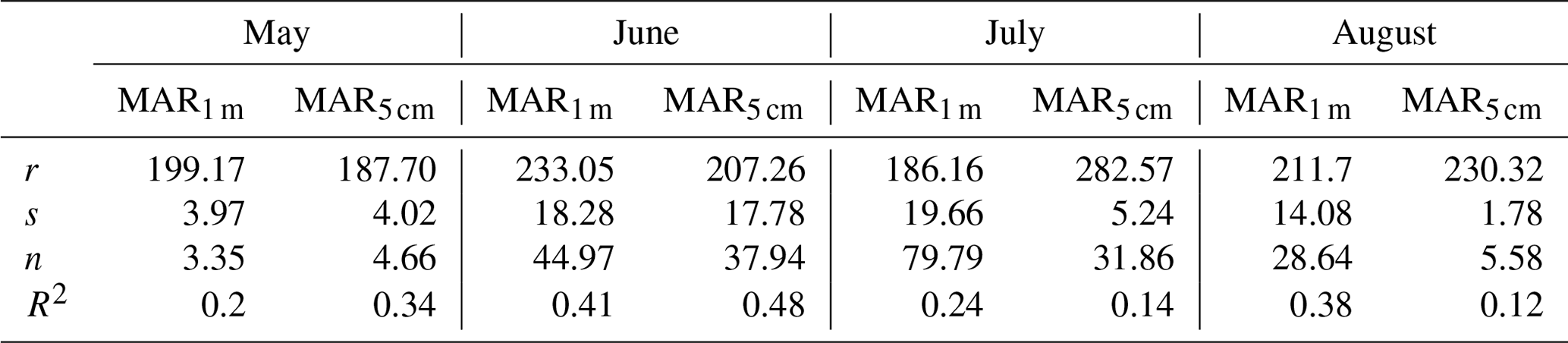
Figure 11 Empirical (blue crosses) and modeled (red line) semi-variograms for the Greenland melt duration (MD) computed by applying the (a, b) MEMLS and (c, d) 245 K algorithms to both the (a, c) 25 km and (b, d) 3.125 km resolution data for each month of the melting season (May, June, July and August). The range (r), sill (s), nugget (n) and R² values are reported.

4 Conclusions and future work

We applied threshold-based melt detection algorithms to the 3.125 km resolution 37 GHz horizontally polarized PMW T_b to assess the skill of the PMW enhanced-resolution data to detect surface melting for the 1979–2019 period over the Greenland ice sheet. As the product is composed of data acquired by different sensors on board different platforms, we first developed a cross-calibration among all of the sensors. We then compared surface melting detected from PMW enhanced-resolution data with that estimated from AWS air temperature data and the outputs of the MAR regional climate model. We found that the algorithm making use of a fixed threshold value for T_b values (245 K) and the algorithm based on the outputs of an electromagnetic model were the most suitable for detecting persistent (245 K) and sporadic (MEMLS) melting. Overall, we found that the MEMLS algorithm showed the best performance (lowest commission and omission errors). We compared surface melting detected from PMW enhanced-resolution data with that estimated by the MAR model when considering the two cases of integrating LWC over the top 5 cm and 1 m, respectively. We selected these two depths to study conditions in which melting occurs sporadically (5 cm) or persistently (1 m). We obtained a good match (i.e., NSE > 0.4 or, at least, positive) in most of the years from 1992 to 2019 when comparing the MEMLS-derived melt extent with MAR LWC in the first 5 cm of the snowpack. In contrast, we found a bad match between the two in the 1979–1992 period, possibly due to differences in sensor characteristics. For the melt extent retrieved by 245 K, we found a strong underestimation of the melt extent (largely negative NSE coefficient values) from 1979 to 1987 that was likely due to the lower values of “wet” T_b for SMMR data; this slightly improved from 1993 to 2019 but was still negative. Accordingly, the results obtained by applying the MEMLS approach are more reliable than those for the 245 K algorithm when considering the 1979–2019 period. In the comparison with the PMW coarse-resolution dataset (25 km), we found that the melt extent time series derived from the PMW enhanced-resolution data using MEMLS showed better agreement with the MAR simulations than those obtained using the 25 km resolution data.

After assessing the outputs of the PMW-based algorithms, we studied the melt onset date, melt end date, mean melt duration and maximum melting surface for the 1979–2019 period. According to the MEMLS algorithm, we found that the melting season began 0.404 (0.254) d earlier every year between 1979 and 2019 (1988–2019) and ended 0.708 (0.396) d later every year between 1979 and 2019 (1988–2019). These values are averaged over the whole ice sheet, and the trends are statistically significant at a 95 % level (p value < 0.05). The mean melt duration increased every year by 0.451 d yr⁻¹ (0.291 d yr⁻¹) during the 1979–2019 (1988–2019) period. We found differences in trends computed using the PMW coarse-resolution data with respect to the PMW enhanced-resolution data for the 1979–2012 and 1988–2012 reference periods, possibly because of the different rationale behind the melt detection algorithms and the higher level of detail in the PMW enhanced-resolution dataset. When we performed a spatial analysis of the trends for the melt onset dates and duration, we found that the areas where the number of melting days has been increasing are mostly located in western Greenland. The maximum melting surface also presents positive trends, with an increment of 0.69 % (0.36 %) every year with respect to the Greenland ice sheet surface since 1979 (1988).

Finally, we explored the information content of the PMW enhanced-resolution dataset with respect to the one at 25 km and the MAR outputs using a semi-variogram approach. The results obtained showed a better fitting of the modeled spherical function to the empirical semi-variogram for the enhanced-resolution data and MAR maps of melt duration. Our analysis suggests that the enhanced-resolution product is sensitive to local-scale processes, with higher sensitivity in the case of the MEMLS algorithm. This offers the opportunity to improve our understanding of the spatial scale of the processes driving melting and potentially paves the way for the use of this dataset in statistically downscaling model outputs. In this regard, as a future work, we plan to extend the analysis of spatial scales to the atmospheric drivers of surface melting, such as incoming solar radiation, surface temperature and longwave radiation, and to complement this analysis with our previous work, which is focused on understanding the changes in atmospheric patterns that have been promoting enhanced melting in Greenland over the recent decades (Tedesco and Fettweis, 2020). As we have assessed the capacity of this dataset and method to observe temporal trends, further development could include a combination of the PMW enhanced-resolution dataset with higher-resolution satellite data (optical sensors or lower frequencies) in order to investigate the evolution of the surface meltwater networks and the application of similar tools to other regions, such as the Canadian Arctic Archipelago, the Himalayan Plateau and the Antarctic Peninsula, where the enhancement of the spatial resolution could be fully exploited.