the Creative Commons Attribution 4.0 License.
the Creative Commons Attribution 4.0 License.
 | 04 May 2021
Linking sea ice deformation to ice thickness redistribution using high-resolution satellite and airborne observations
Luisa von Albedyll
Christian Haas
Wolfgang Dierking
An unusual, large, latent-heat polynya opened and then closed by freezing and convergence north of Greenland's coast in late winter 2018. The closing presented a natural but well-constrained full-scale ice deformation experiment. We observed the closing of and deformation within the polynya with satellite synthetic-aperture radar (SAR) imagery and measured the accumulated effects of dynamic and thermodynamic ice growth with an airborne electromagnetic (AEM) ice thickness survey 1 month after the closing began. During that time, strong ice convergence decreased the area of the refrozen polynya by a factor of 2.5. The AEM survey showed mean and modal thicknesses of the 1-month-old ice of 1.96 ± 1.5 m and 1.1 m, respectively. We show that this is in close agreement with modeled thermodynamic growth and with the dynamic thickening expected from the polynya area decrease during that time. We found significant differences in the shapes of ice thickness distributions (ITDs) in different regions of the refrozen polynya. These closely corresponded to different deformation histories of the surveyed ice that we reconstructed from Lagrangian ice drift trajectories in reverse chronological order. We constructed the ice drift trajectories from regularly gridded, high-resolution drift fields calculated from SAR imagery and extracted deformation derived from the drift fields along the trajectories. Results show a linear proportionality between convergence and thickness change that agrees well with the ice thickness redistribution theory. We found a proportionality between the e folding of the ITDs' tails and the total deformation experienced by the ice. Lastly, we developed a simple, volume-conserving model to derive dynamic ice thickness change from the combination of Lagrangian trajectories and high-resolution SAR drift and deformation fields. The model has a spatial resolution of 1.4 km and reconstructs thickness profiles in reasonable agreement with the AEM observations. The modeled ITD resembles the main characteristics of the observed ITD, including mode, e folding, and full width at half maximum. Thus, we demonstrate that high-resolution SAR deformation observations are capable of producing realistic ice thickness distributions.
- Article
(8788 KB) - Full-text XML
-
Supplement
(900 KB) - BibTeX
- EndNote


Sea ice thickness is a key climate variable because it governs the mass, heat, and momentum exchange between the ocean and the atmosphere (e.g., Maykut, 1986; Vihma, 2014). A superposition of thermodynamic processes, i.e., growth or melt, and ice dynamics, i.e., advection and deformation of ice, controls sea ice thickness. Both thermodynamics and mechanics alter depending on sea ice thickness.
The interplay of dynamics and thermodynamics results in large thickness variations, and ice thickness distributions (ITDs) are used to characterize them. Thermodynamic processes modify ice thickness slowly depending on the surface energy balance, and growth is limited to the equilibrium thickness (Maykut, 1986). Since the atmospheric and oceanic forcing varies little on sub-regional scales, the most frequent, i.e., the modal, thickness of an ITD often represents the undeformed, thermodynamically grown level ice (Wadhams, 1994; Thorndike, 1992; Haas et al., 2008).
In contrast, deformation caused by differential ice motion leads to abrupt changes in ice thickness. Driven by winds, ocean currents, and tides and constrained by coasts and the internal stress of the ice pack, divergent motion creates areas of open water, e.g., leads and polynyas, and reduces thickness to zero. Convergent motion results in the closing of leads and then rafting and ridging of young and old ice. Ridging of thick ice forms pressure ridges that are many times thicker than the initial thickness (Strub-Klein and Sudom, 2012; Duncan et al., 2020). Ridging and rafting shape the ITD predominantly by redistributing thin ice to thicker ice categories (e.g., Thorndike et al., 1975; Wadhams, 1994; Rabenstein et al., 2010).
The ITD is a key parameter in the parameterization of many climate and weather-relevant processes. For example, effective heat transfer between the ocean and atmosphere is limited to thin ice. Hence, knowledge of the ITD is crucial for realistic short- and long-term model predictions of sea ice thickness and volume (Kwok and Cunningham, 2016; Lipscomb et al., 2007).
Submarine and satellite-based observations have shown a substantial decline in sea ice thickness in the Arctic Ocean within the last 6 decades (Lindsay and Schweiger, 2015; Kwok, 2018). At the same time, sea ice drift speeds have increased significantly, indicating enhanced ice deformation (Spreen et al., 2011; Rampal et al., 2009). In the context of those changing Arctic conditions with reduced net thermodynamic growth and ice thickness, the contribution of dynamic processes to sea ice thickness might gain more importance (Itkin et al., 2018).
However, the interdependency between sea ice thickness and enhanced sea ice dynamics is not yet well understood. Most apparently, the reduction in the material strength of the ice associated with its thinning is suspected to increase deformation (Rampal et al., 2009). As a more fractured ice cover is easier to move, this may explain the substantial increase in sea ice drift speed (Rampal et al., 2009). In the Transpolar Drift, enhanced ice drift speeds even accelerate the loss of thicker, multi-year ice (MYI) through the Fram Strait (Nghiem et al., 2007). On the other hand, the reduced ice strength and higher drift speed leads to an increase in deformation that is of great importance in producing a thick ice cover through ridging (Itkin et al., 2018; Kwok, 2015; Rampal et al., 2009).
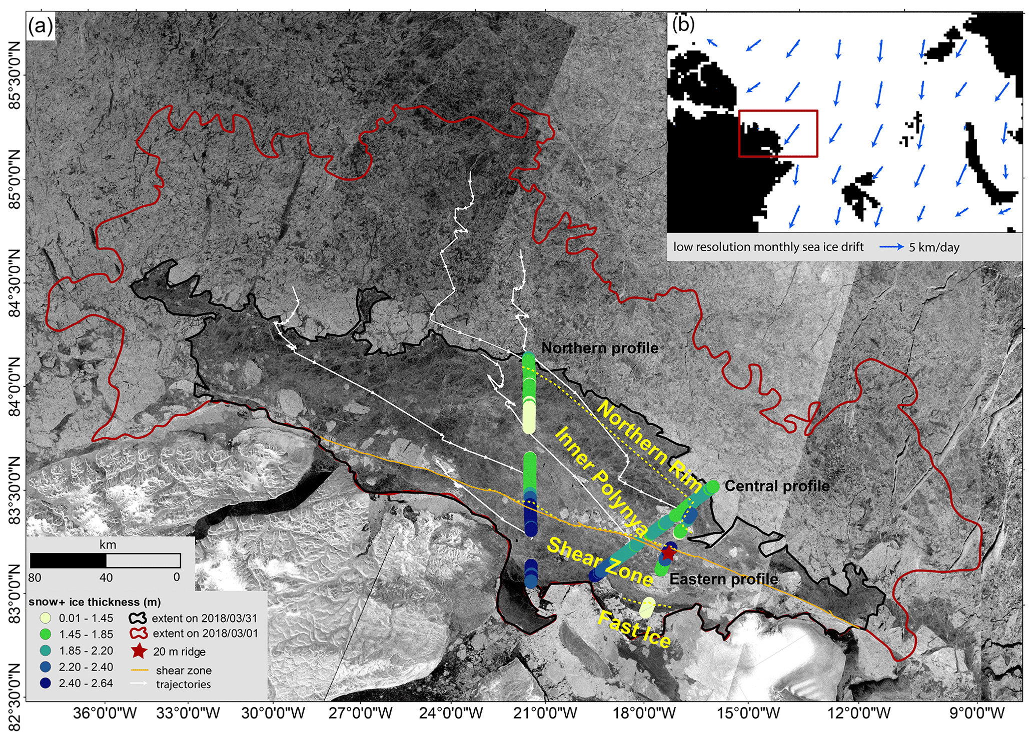
Figure 1Ice thickness survey of the first-year ice (FYI) in the refrozen polynya off the coast of North Greenland in March 2018. (a) Sentinel-1 SAR Extra Wide Swath HH-polarization image acquired on 31 March 2018, shown on a decibel scale. The dark-gray areas are heavily deformed FYI between brighter multi-year ice (MYI) (upper image part and embedded in the FYI) and the coast of Greenland (lower part). Red and black lines outline the extents of the refrozen polynya on 1 and 31 March 2018. A sequence of white arrows illustrates four ice drift trajectories derived from daily velocity fields (Sect. 2.5), representing the typical southeasterly ice movement during the convergent closing of the polynya. The orange line marks the large-scale shear zone, and the red star marks the location of a 20 m thick ridge. Colored circles represent the 15 km running mean of the FYI snow and ice thicknesses. We chose the non-linear color scale to stress the differences in mean thickness between 1.4 and 2.4 m (see Table 1). Dashed yellow lines show four distinct zones with different mean thicknesses and deformation histories: thin ice in the weakly deformed Fast Ice; thick ice in the severely deformed Shear Zone; moderately deformed, thin ice in the Inner Polynya; and strongly deformed, thick ice in the Northern Rim. (b) Overview map with monthly averaged, low-resolution sea ice drift in March 2018 (not showing the local drift variability in the polynya, drift from NSIDC Polar Pathfinder; for details, see “Data availability” at the end of the text). The red box marks the region shown in (a).
It remains challenging to quantify the net effects of changes in sea ice dynamics on sea ice thickness and volume change. The existing redistribution theory that links deformation and thickness change is not yet well constrained by observations (Lipscomb et al., 2007; Thorndike et al., 1975; Hibler, 1979). Two recent studies, a short-term, local-scale study based on airborne laser scanning (Itkin et al., 2018) and a long-term, basin-wide study based on CryoSat-2 ice thickness retrievals (Kwok and Cunningham, 2016), provided observational evidence for a linear proportionality between deformation and dynamic thickness change. Using RADARSAT Geophysical Processor System (RGPS) drift and deformation, Kwok (2002) has shown that SAR-derived dynamic thickness change of the seasonal ice cover results in reasonable estimates of the ice thickness.
Here, we present a regional case study of sea ice deformation and its impacts on dynamic ice thickness change and redistribution using satellite synthetic-aperture radar (SAR) data and airborne electromagnetic (AEM) ice thickness observations. We have studied refreezing and convergence of ice that had formed in an unusual latent-heat polynya that occurred along the north coast of Greenland in the late winter of 2018 (Ludwig et al., 2019; Moore et al., 2018; Fig. 1). In February 2018, strong and persistent northward winds over the Greenland Sea reversed the normally coastward direction of the large-scale ice drift close to northeast Greenland and thus pushed the common, thick coastal multi-year ice northward, opening up a coastal polynya (Moore et al., 2018; Ludwig et al., 2019). The polynya reached its maximum size of approximately 65 000 km2 on 25 February 2018 (Moore et al., 2018). The observed sea ice concentration was unusually low for this area and time (Ludwig et al., 2019). While the open-water area quickly refroze due to air temperatures well below the freezing point, the convergent motion of the surrounding multi-year ice driven by coastward-directed, i.e., southward, winds decreased the area of the refreezing polynya and deformed the newly formed ice heavily, thereby strongly impacting its thickness. One month after the maximum extent of the polynya, we carried out an AEM ice thickness survey over the refrozen polynya. The thickness observations captured the integrated effects of the thermodynamic and dynamic thickness changes of the event.
In this paper we provided a detailed analysis of deformation derived from SAR imagery and related it to the resulting ice thickness distributions obtained from the AEM surveys. We focused on three aspects: first, we related the large-scale area decrease of the refrozen polynya to the observed average thickness and showed that dynamic processes contributed about 50 % of the observed mean thickness. Second, we related the regional variability in mean thickness and the shape of the ITD to differences in regional deformation observed by SAR ice drift tracking. We established relationships between key properties of the ITD like mean thickness and e folding and deformation. Third, we demonstrated that high-resolution deformation derived from SAR images can be used to calculate dynamic thickness change. Under some general assumptions summarized in a simple, ice-volume-conserving model, we could reproduce a realistic ITD.
We based our work on AEM ice thickness measurements (Sect. 2.1) and SAR-derived deformation observations and proceeded as follows:
-
We quantified the thermodynamic growth from a model simulation (Sect. 2.2) and the large-scale dynamic thickness increase in the refrozen polynya from the decrease in the area covered by the refrozen polynya (Sect. 2.3).
-
We derived divergence and shear from SAR-derived sea ice motion fields (Sect. 2.4) to analyze local, spatial variability in deformation and thickness within the polynya. We reconstructed Lagrangian trajectories of the surveyed ice parcels in a reverse timeline to disentangle the ice parcel's individual deformation history (Sect. 2.5).
-
We used a simple, volume-conserving ice thickness model to calculate ice thickness along the Lagrangian trajectories. We forced the model with the SAR-derived high-resolution deformation fields (Sect. 2.6). To evaluate the model results, we compared the modeled thicknesses with the AEM thickness observations.
2.1 Ice thickness measurements
On 30 and 31 March 2018, the Alfred Wegener Institute's research aircraft Polar 5 conducted two AEM ice thickness survey flights over the refrozen polynya and the surrounding MYI. A total of 230 km of thickness profiles of predominantly first-year ice (FYI) was obtained along three profiles: a northern, central, and eastern profile. The AEM surveys recorded total (snow and ice) thickness with a point spacing of approximately 6 m (Fig. 1a).
AEM thickness retrievals find the distance to the strongly conducting seawater under the ice. A laser altimeter provides the distance to the upper snow surface, and subtraction of these two distances gives the combined snow and ice thickness (Haas et al., 2006; Pfaffling et al., 2007; Haas et al., 2009). The footprint of the measurements was approximately 40–50 m, and the uncertainty is generally estimated to be ± 0.1 m over level ice (Haas et al., 2009). The footprint smoothing underestimates the maximum ridge thickness but overestimates the ridge flanks. When averaging over longer distances of ridged ice, the two effects compensate for each other such that the mean thickness is found to be in close agreement with drill-hole measurements (Pfaffling et al., 2007; Hendricks, 2009; Haas et al., 1997). Details on the data processing are provided in Haas et al. (2009).
To evaluate snow contribution to the observed total thickness, we analyzed snow thickness from Operation IceBridge (OIB) Sea Ice Freeboard, Snow Depth, and Thickness Quick Look data (for details, see “Data availability” at the end of the text). They surveyed the refrozen polynya on 22 March 2018. We note that OIB's observed modal snow thickness of 4 cm (mean 9 cm) agrees well with the expected accumulation between February and March from the Warren climatology (Warren et al., 1999). However, we also take into account that OIB Sea Ice Freeboard, Snow Depth, and Thickness Quick Look data most likely underestimate snow thickness on the order of 5–6 cm (King et al., 2015).
Meteorological observations at Villum Research Station (Station Nord; 81∘36′ N, 16∘40′ W) indicate no further significant snowfall between 22 and 30/31 March 2018, when the AEM surveys took place. Since the measurement uncertainty in the electromagnetic (EM) instrument lies above the estimated snow thickness, we refrain from correcting the total thickness for snow. Hence, we consider the thickness measured by the EM instrument as ice thickness. The uncertainty in the AEM principle (0.1 m) and the snow thickness (0.04 m) add up to ± 0.14 m uncertainty in the AEM ice thickness measurements. We note that local snow thickness variability, especially close to ridges, adds additional, spatially highly variable uncertainty to the thickness measurements.
Since our study focuses on the evolution of the ice that was formed and deformed during the closing of the polynya, we separated MYI from the newly formed FYI in the refrozen polynya. We used SAR images to identify the northern, outer boundary of the polynya visually. The boundary is clearly visible because of the strong radar backscatter contrast between the FYI (low backscatter) and MYI (high backscatter, Fig. 1; see video supplement 1). Several MYI floes were located within the polynya. We traced them back in time on the SAR images to be sure that they were MYI, i.e., that they were present before the polynya formation. We combined this information with the thickness profiles and the backscatter of the SAR images on 31/30 March 2018. We excluded the MYI floes from the AEM profiles flown over the refrozen polynya area but used the MYI floes to validate the tracking algorithm. All following considerations relate only to FYI unless specified differently. After removing data gaps and MYI ice from the thickness profiles, the total profile length over the FYI was 180 km.
We used mean and modal thickness to characterize the ice thickness distributions, where the latter was calculated based on a bin width of 20 cm. We considered ice thinner than 10 cm open water. We characterized the tail of the ITD by the e-folding λ of an exponential fit to all the ice categories of the ITD thicker than the modal thickness hmode. The exponential fit has the form , where h is the thickness of the different bins and a is a fitted parameter. The full width at half maximum (FWHM) characterizes the width of the ITD where it is at 50 % of the maximum. We take large values of e folding and the FWHM as an indicator of enhanced ice deformation.
We identified sections of level, undeformed ice along the profiles surveyed by Polar 5 by applying a modified version of the level ice filter suggested by Rabenstein et al. (2010). The filter identifies level ice based on two criteria. First, the vertical thickness gradient along the thickness profile is smaller than 0.006, and second, this condition is met continuously for at least 40 m of profile length, a parameter that was chosen to approximate the footprint of the AEM measurements. The approach is more restrictive than other identification schemes (e.g., Wadhams and Horne, 1980) but well suited to minimizing the amount of deformed ice wrongly passing the filter (Rabenstein et al., 2010).
2.2 Thermodynamic ice thickness growth
We aim at separating the dynamic and thermodynamic contributions to the overall thickness. For the thermodynamic growth, we carried out a dedicated thermodynamic model experiment of the refreezing polynya. Instead of applying a freezing-degree-day model like, e.g., that of Ludwig et al. (2019), we used a regional setup of the coupled ocean and sea ice configuration of the Massachusetts Institute of Technology general circulation model (MITgcm; e.g., Losch et al., 2010). The model domain comprised the polynya region and surrounding MYI. The model was run with two-category, zero-layer thermodynamics (Menemenlis et al., 2005; Semtner, 1976) and forced with hourly re-analysis data (ERA5) with a spatial resolution of 31 km. We started the model with an initial ice thickness of 0 m in the polynya on 25 February 2018, when the polynya had reached its maximum extent, and ran it until 31 March 2018. We ran the model without sea ice dynamics in the polynya region, enabling us to separate the contribution of the thermodynamic growth (hth) from the daily total spatial means of ice thickness within the polynya.
2.3 Large-scale dynamic thickness change due to area decrease of the FYI in the closing polynya
The magnitude of deformation is related to the area decrease of the closing polynya. Therefore, we identified the area of the FYI on near-daily Sentinel-1 SAR images from 25 February to 31 March 2018 (Figs. 1, 4a; see video supplement 1). We visually identified the extent of the gradually closing polynya by tracking the edge between the FYI area characterized by low radar backscattering and the adjacent MYI with higher backscattering. For the area calculation, we excluded the area of the MYI floes located within the FYI (see Sect. 2.1).
As a first approximation we assumed ice volume conservation; i.e., the average dynamic ice thickness increase is proportional to the average area (A(tk)) decrease at time tk. Hence, we estimated the mean (dynamic and thermodynamic) thickness by
where n=34 is the total number of days considered in this study, k=0 refers to 25 February 2018, and k=34 refers to 31 March 2018. We modeled the thermodynamic growth between tk and tk+1 () with the MITgcm pure thermodynamic run (Sect. 2.2, Fig. 4). Note that the thermodynamic growth (from the MITgcm) is uncoupled from the dynamic changes because dynamics were switched off in the model run. Hence, we did not account for reduced ice growth as the mean thickness increased.
2.4 Sea ice drift and deformation from sequential SAR images
We computed ice drift fields with an ice tracking algorithm introduced by Thomas et al. (2008, 2011) and modified by Hollands and Dierking (2011). The algorithm identifies patterns of radar backscatter coefficients in sequential SAR images and estimates the spatial displacement of those patterns between the images. The algorithm is based on multi-scale, multi-resolution pattern matching, offering high robustness at reasonable computational costs (Hollands and Dierking, 2011). Drift fields were obtained from Sentinel-1 HH-polarized radar intensity images that were acquired in Extra Wide Swath mode with a pixel size of 50 m. Pre-processing was carried out with the ESA SNAP software package and included thermal noise removal, image calibration, refined Lee speckle filtering (7×7 pixels), and a coastline terrain correction. The time steps between two scenes used to derive ice drift varied between 0.9 and 2 d. The final drift data set is defined on a regularly spaced grid with a spatial resolution of 700 m. We filtered the data with a 3×3-point running-median filter covering an area of 2.1×2.1 km, which efficiently isolates outliers covering 1 pixel while preserving sharp gradients in the velocity field.
We calculated sea ice deformation from the spatial derivatives of the gridded u (velocity in the x direction) and v (velocity in the y direction) components of the spatially filtered velocity field () by convolution with a 3×3 Sobel filter (kx). For example, is obtained from
where Δy is the grid spacing in the y direction, i.e., 700 m. For a regularly spaced grid this calculation to derive deformation is identical to the commonly used equations for a combination of 2×2 adjacent velocity grid cells, which are based on Green's theorem. (see Supplement and, e.g., Kwok et al., 2003, 2008; Dierking et al., 2020). The velocity gradients were evaluated every 700 m, corresponding to a step width of one grid cell. Divergence rate (), shear (), and total deformation () were derived from the spatial velocity gradients using
2.5 Lagrangian ice drift trajectories
We aimed at attributing differences in the regional thickness variability measured by the AEM surveys to differences in the deformation history of the respective ice parcels. To obtain information on the drift of those, we reconstructed Lagrangian ice drift trajectories of the surveyed ice parcels using a reverse timeline, as follows:
-
As starting point of the tracking, we down-sampled the spatial resolution of the thickness profiles surveyed on 30/31 March 2018, to 250 m. Occasional gaps in the thickness observations increased the distance between the starting points to up to 350 m. Next, we corrected the GPS data of the AEM measurements for the ice displacement that took place between the time of the AEM survey and the acquisition of the satellite images (maximum 6 h). In total, we initiated the tracking at 715 down-sampled points along the AEM profiles surveyed on 30/31 March (Fig. 1).
-
We reconstruct the trajectory of each ice parcel by interpolating the regularly spaced velocity field to the end position at a given time step and adding the respective displacement to determine the end position for the next time step. As examples, four of the reconstructed trajectories are displayed as thin white lines in Fig. 1a.
-
For each time step, which was typically 1 d, we extracted divergence, shear, and total deformation from the deformation fields calculated based on the drift fields (Sect. 2.4) around the end position of the respective trajectory. We used the trajectories to identify the ice's position within the deformation field but not to calculate deformation based on them.
-
We performed the backward Lagrangian tracking from 30/31 until 1 March 2018. We chose 1 March 2018 as the last day of the backtracking because, before this date, the new ice in the polynya was not consolidated and did not reveal recognizable backscatter patterns for retrieving ice drift.
Uncertainty in deformation estimates along the ice drift trajectories
Uncertainties in the initial ice velocity fields propagate into the deformation estimates along the trajectories in three different ways.
-
The tracking error results from incorrect pattern matching, e.g., due to a lack of recognizable and stable spatial radar signature variations. Hollands and Dierking (2011) found tracking errors of between ± 0.8 and ± 1.6 pixels (their Tables 3 and 4, standard deviations). For a pixel size of 50 m this corresponded to ± 40–80 m. However, the tracking errors along a trajectory in a spatially inhomogeneous velocity field do not simply add up but can be reinforced. We estimated this accumulated trajectory position error from manual tracking of MYI floes located in the polynya (see Fig. 1a). After the second time step, the accumulated trajectory position error was on average 51 m, with a maximum of 210 m (see Supplement). At the end of the tracking (1 March 2018), the accumulated trajectory position error was on average 1050 m, with a maximum of 2150 m. We interpret the accumulated trajectory position error as an increasing area (circle) around the Lagrangian ice drift trajectory, in which the true position of the ice parcel is located (see Supplement for details). We extracted divergence, shear, and total deformation from all deformation cells whose center points fell into this uncertainty circle (Fig. 2a).
-
Random errors in the velocity field introduce statistical errors in the deformation parameters. To reduce them, we applied the concept of back-matching, which, e.g., Hollands et al. (2015) used to judge the reliability of the retrieved drift vectors. In back-matching, the drift is retrieved from a second time by reversing the order of image 1 and image 2. The effect is that the positions of the windows used for pattern matching are different between combinations 1–2 and 2–1. In zones of small differences between both drift fields, we calculated and extracted deformation from the forward and backward deformation fields. Zones with large differences are regarded as unreliable and not considered.
-
The third source of errors for deformation calculations, the boundary definition error, is related to the discretization of an inhomogeneous velocity field into grid cells and is difficult to quantify (Griebel and Dierking, 2018; Lindsay and Stern, 2003). Griebel and Dierking (2018) showed that the boundary definition error could be reduced by a factor of about 2 if the deformation is calculated from the velocity gradients at the margin of a 2×2 cluster of grid cells instead of using only one grid cell. This approach is also used here (see Sect. 2.4).
Considering the errors mentioned above, we used the following approach for calculating possible thickness variations along a trajectory. We extracted divergence from the forward and backward deformation fields (see 2. above) of all grid cells in the circles of uncertainty (see 1. above) along the trajectories (Fig. 2a). We created, for each of the 715 trajectories, 10 000 random combinations of the potentially experienced divergence magnitudes within the uncertainty circles.
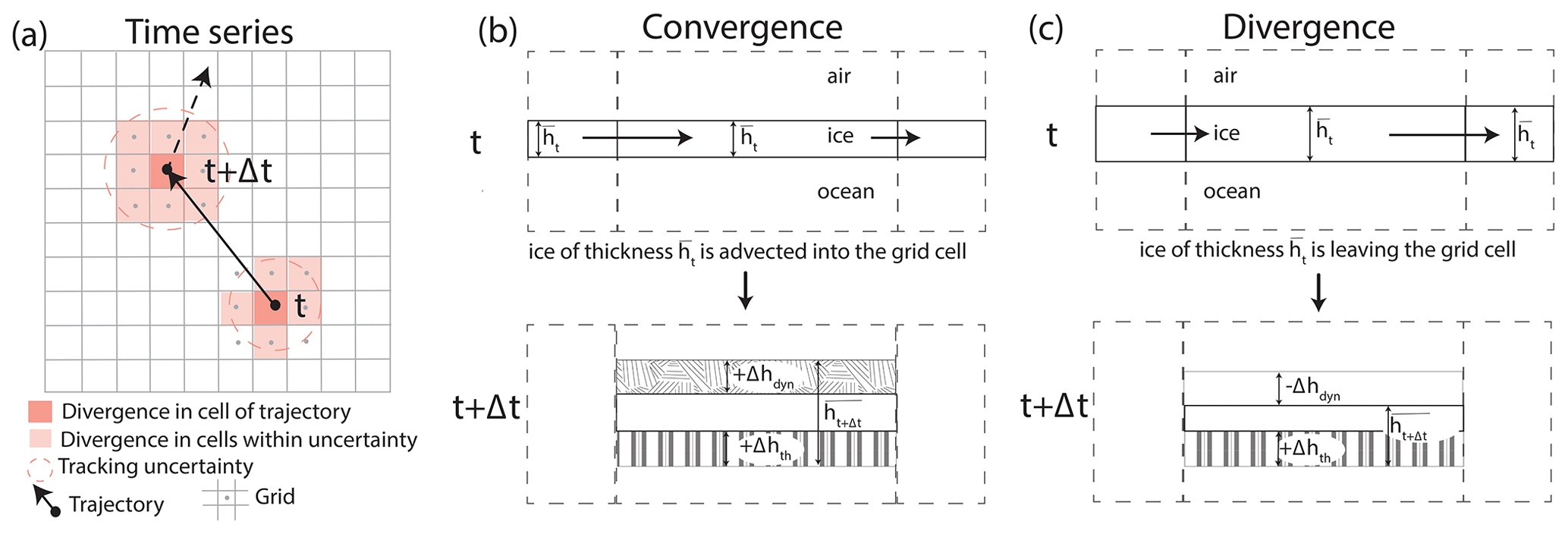
Figure 2Sketch of the simple ice thickness model showing the vertical cross section of thickness change between time steps t and t+Δt. (a) Trajectories on deformation grid. The deformation grid defines the grid cells as sketched in (b) and (c). Divergence is extracted from all grid cells whose center points (gray dots) are located in the uncertainty range given by the increasing accumulated trajectory position error (dashed circle). (b) In the case of convergence, ice with a mean grid cell thickness is advected into the grid cell, resulting in a volume-conserving thickness increase (+Δhdyn). (c) In the case of divergence, ice with a mean thickness leaves the grid cell, reducing ice thickness dynamically by −Δhdyn. Thermodynamic growth +Δhth continues unabatedly in (b) and (c), independently of deformation.
2.6 Ice thickness change along trajectories modeled with a simple, volume-conserving model
Based on the basic principles of thermodynamic and dynamic ice thickness changes described by Thorndike et al. (1975) and Hibler (1979), we modeled dynamic thickness change from deformation (Fig. 2). With the model, we aimed to demonstrate in the most simple framework that deformation derived from high-resolution SAR images is capable of reproducing realistic dynamic ice thickness changes. The simple model is a one-layer, volume-conserving model. We applied it along each trajectory to simulate the mean thickness of a grid cell (1.4×1.4 km) from thermodynamic growth, advection, and ice deformation (Fig. 2a). The model does not include any ridging scheme.
Our model is based on the redistribution theory introduced by Thorndike et al. (1975) and simplified for the mean thickness by, e.g., Hibler (1979):
Here, the thermodynamic growth or melt rate (±Δhth) and advection of ice, given by the divergence term (−div(vh)) of the velocity field v and the ice thickness h, alter the mean thickness as shown in Fig. 2b and c. This equation does not consider ice density changes, for example, due to the porosity of pressure ridges (Flato and Hibler, 1995). Since we modeled ice thickness along Lagrangian ice drift trajectories, the advection term can be written as (e.g., Thorndike, 1992). Note that according to Eq. (4), mean thickness change is proportional to the divergence of the velocity field.
We made the following assumptions about the ice properties: first, we determined the thickness h of the ice advected into the grid cell. Due to the high spatial resolution, neighboring grid cells have a common thermodynamic and dynamic growth history, which is why their mean thicknesses are similar. Hence, we approximated the thickness of the advected ice h by the mean thickness of the grid cell at time t (see Fig. 2).
Second, we approximated the thermodynamic ice growth Δhth within the grid cell in Eq. (4) by the growth of the undisturbed, thermodynamically growing ice obtained from the thermodynamic MITgcm run (Sect. 2.2; Fig. 2b, c). We based this assumption on the observation that deformation changes the thickness only very locally, affecting only a small portion of the grid cell while thermodynamic growth continues unabatedly under the remaining level ice. We are aware that this underestimates (overestimates) ice growth in grid cells that experienced strong divergence (convergence). Divergence generates open water where thermodynamic growth is strongly enhanced. Convergence may create such thick ice that the thermodynamic growth is reduced or even reverted to melt (see Sect. 4.3 in the Discussion).
Based on Eq. (4) we obtain the mean thickness at each time by
where t runs from 1 to 31 March 2018 and the time steps Δt are typically 1 d.
To account for the uncertainties in the drift and deformation, we calculated for each of the 715 trajectories mean thickness and standard deviation as uncertainty from the 10 000 thickness estimates obtained from the 10 000 random combinations of divergence (see Sect. 2.5.1). In 5 % of the calculations, divergence caused the ice thickness in a grid cell to drop below 0. To prevent grid cells that contain only open water (zero thickness) from accumulating “negative thickness” when divergence continues, we reset the accumulated thickness to zero.
In this section, we first quantify the large-scale dynamic thickness change that is linked to the decrease in the refrozen polynya area (Sect. 3.1). Second, we analyze the spatial thickness variability in the refrozen polynya and demonstrate that it can be attributed to local differences in the deformation (Sect. 3.2). Grouping the ice thickness observations by their deformation history, we establish links between the shape of the ITD and the magnitude of deformation (Sect. 3.3). Finally, we apply the simple volume-conserving model to derive dynamic thickness change from deformation along ice drift trajectories and evaluate our results by comparison with the observed thicknesses (Sect. 3.3).
3.1 Thermodynamic and large-scale dynamic thickness change
The AEM thickness surveys showed that after only 1 month of ice growth, the newly formed FYI had a mean thickness of 1.96 ± 1.5 m and a mode of 1.1 m (center of bin width 1.0–1.2 m), including 1.5 % of open water (Figs. 1d, 3a). The asymmetric shape of the ITD (Fig. 3, Table 1), with most of the ice (78 %) thicker than the mode, clearly documents the impact of deformation. Convergence redistributed thinner ice into thicker ridges of up to 20 m thickness. As a result, there is a large difference of approximately 0.9 m between the mean and modal thickness, where the latter is considered a good approximation for thermodynamically grown, undeformed ice (see Sect. 1). We approximated the long tail of the ITD with an exponential function that had an e folding of 1.04 (see Table 1). The low percentage of 14 % level ice on the three (northern, central, and eastern) profiles provides further evidence of a large amount of deformed ice.
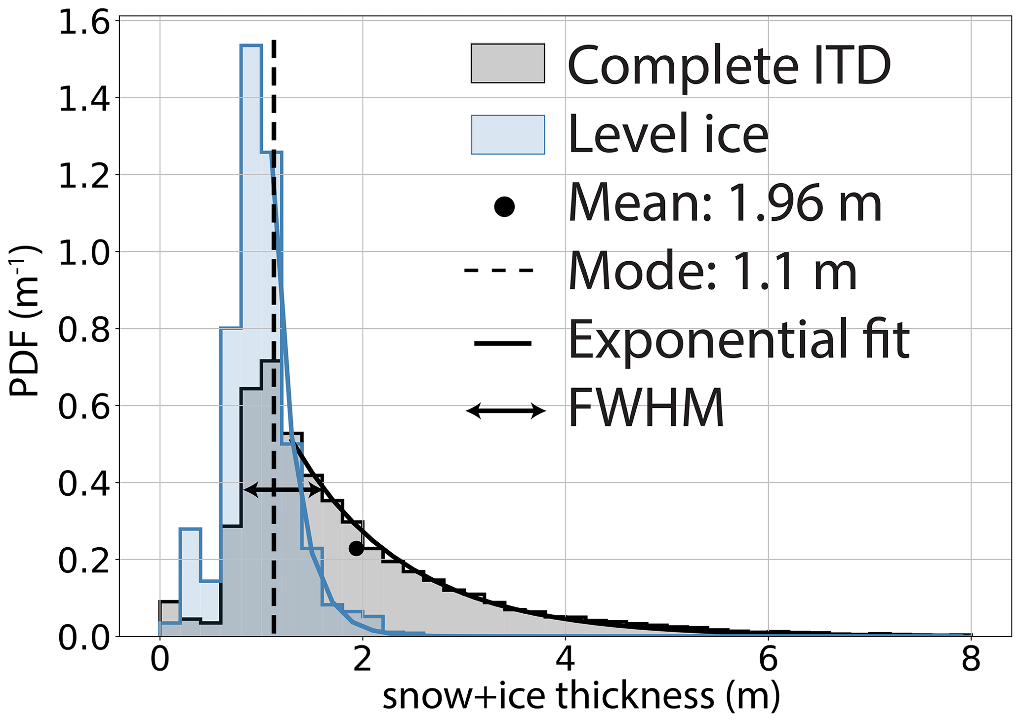
Figure 3Ice thickness distributions (ITDs) displaying snow and ice thickness and observed by AEM on 30/31 March. ITD over the entire area of the refrozen polynya (black) and ITD of the level ice only (blue). Mean, mode, exponential fit, and FWHM are indicated for the former case. Ice thicker than 8 m was observed for less than 1 % of the refrozen polynya area.
3.1.1 Large-scale thermodynamic thickness change
The MITgcm thermodynamic model gives a thermodynamic ice thickness of 0.87 ± 0.03 m on 31 March. The result is in good agreement with the mode of the ITD only considering level ice, which is 0.9 m (Fig. 3). The narrow and almost normally distributed ITD of the level ice (Fig. 3) supports our assumption that the thermodynamic growth was relatively uniform in the refrozen polynya. We suggest that the small spread around the mode is due to undeformed ice that started to grow before or after 25 February, potentially some early rafting events, and the spatial variability in the thermodynamic growth due to inhomogeneous snow cover. We note that the thermodynamic ice thickness of 0.9 m obtained from the model deviates from the mode of the overall ITD by only one bin, confirming the results of previous studies (e.g., Haas et al., 2008) that the thickness of the thermodynamically grown ice can be approximated reasonably well by the modal thickness of an ITD.
Figure 4a shows the time series of thermodynamic thickness growth from 25 February to 30/31 March. On 1 March, when we started to reconstruct the ice drift trajectories and deformation history, the ice already had a thickness of 0.38 m and grew during our study period thermodynamically by another 0.49 m.
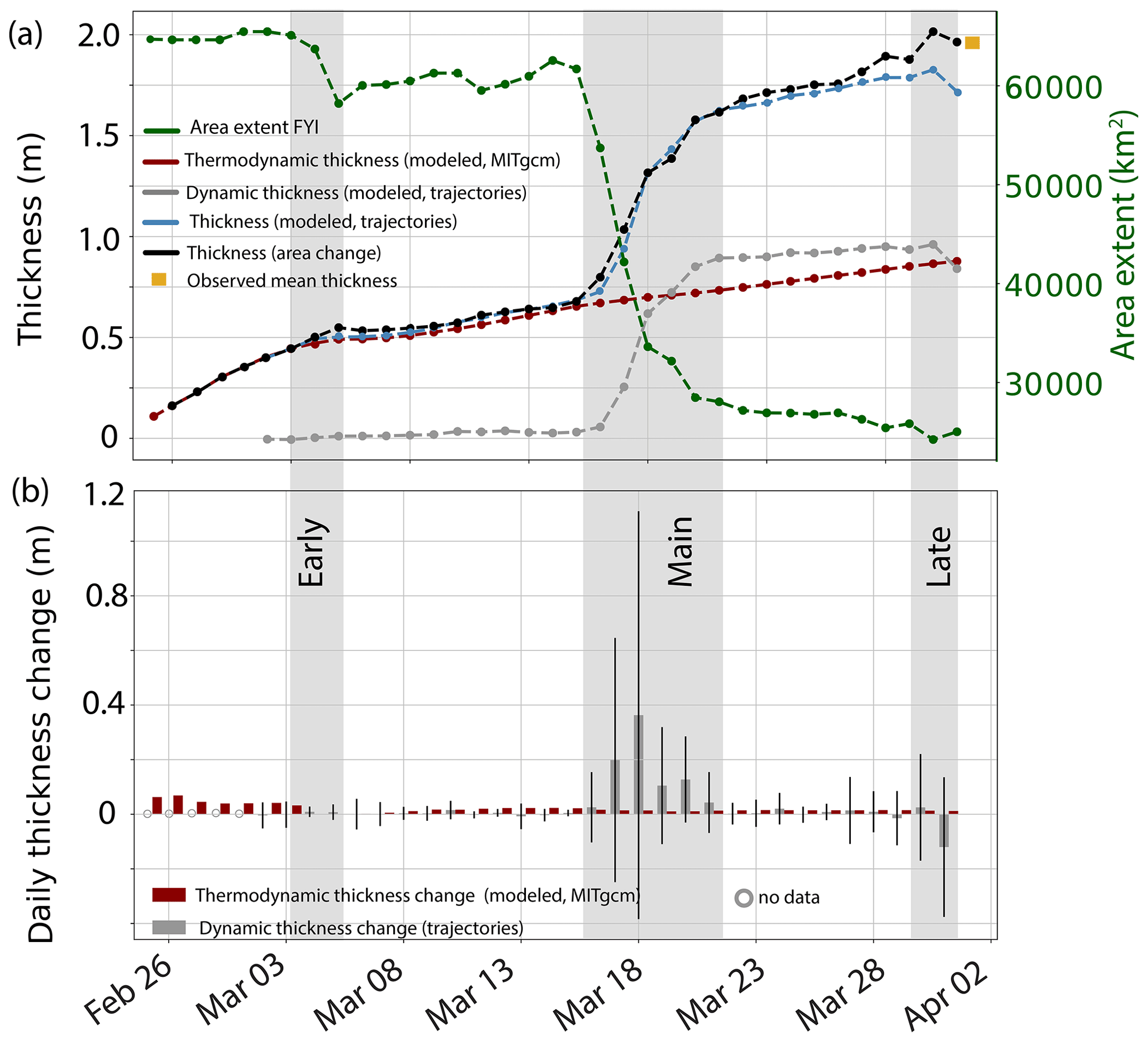
Figure 4Dynamic and thermodynamic contributions to mean thickness from model and observations. (a) Time series of FYI area change (green, right y axis) derived from satellite images. The three deformation phases (early, main, late) are marked in gray. The thickness derived from the area change is shown in black (left axis). Accumulated mean thermodynamic (red, modeled, MITgcm) and dynamic (gray, simple volume-conserving model along trajectories) contribution to the thickness modeled from all trajectories (see b) is displayed in blue. (b) Daily contributions from dynamics (simple volume-conserving model along trajectories) and thermodynamics (modeled, MITgcm) to the overall thickness. Error bars indicate the standard deviation of the dynamic contribution. The new ice that grew in the polynya was 0.38 m thick by 1 March 2018.
3.1.2 Three phases of enhanced area decrease and their impact on mean ice thickness
The shape of the ice thickness distribution showed signs of strong deformation (Sect. 3.1). In the following section, we relate the overall area decrease of the refrozen polynya to the observed thickness change using Eq. (1).
After the polynya had reached its maximum extent on 25 February 2018 (Moore et al., 2018; Ludwig et al., 2019), the usual, large-scale coastward ice drift re-established and persisted through the whole month of March (Fig. 1b). During this time, the area of the FYI decreased by 60 % (video supplement 1, Fig. 4a). The compression took place in three major phases, termed early, main, and late phase (gray areas in Fig. 4, video supplement 2). The active phases were interrupted by quiet phases with weak deformation. The area decrease and deformation observed within the polynya are closely connected to the large-scale ice drift, especially to the magnitude of its coastward component (see insets in Fig. 7). Despite the apparent uniformity of the large-scale forcing, deformation within the polynya showed significant regional variability (see Sect. 3.2, Fig. 7, video supplement 2).
We computed a time series of mean ice thickness using Eq. (1) (Sect. 2.3). We obtained dynamic thickness change from the observed time series of polynya area decrease and modeled thermodynamic growth with the MITgcm (Fig. 4, Sect. 3.1.1). Accordingly, between 25 February and 31 March, this simple approach yielded a mean thickness of m on 31 March, which is consistent with the observed mean thickness along the AEM tracks (Fig. 1d, Table 1). The corresponding time series of mean ice thickness change derived from the area decrease is also displayed in Fig. 4a. From the agreement between the simple approach based on Eq. (1) (Sect. 2.3, last dot of black line in Fig. 4a) and the observed mean thickness (orange square in Fig. 4a), which is excellent here, we conclude that the thermodynamic and dynamic contributions to the mean thickness were 0.9 and 0.96 m, respectively. Further, we note that this excellent agreement is only based on very simple assumptions about thermodynamic and dynamic ice growth.
3.2 Regional differences in ice thickness and deformation within the refrozen polynya
The previous section was concerned with the large-scale, mean dynamic thickness change in the refrozen polynya. In the following, we examine local ice thickness and deformation variations, as well as the potential links between them.
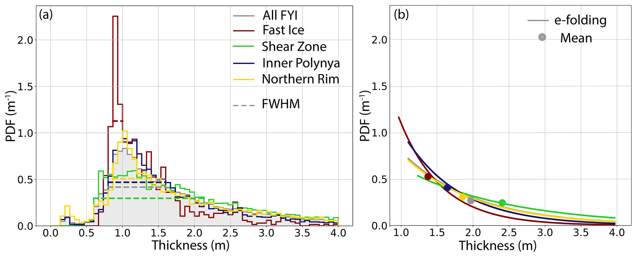
Figure 5ITDs of the four FYI zones of all three AEM lines on 30/31 March 2018. The ITDs differ in (a) FWHM that characterizes the dominance of the mode and (b) mean and e folding of the exponential tail. The ITD of the complete measurements (all FYI) is displayed in gray.
Along all three ice thickness profiles (northern, central, and eastern) from the coast across the refrozen polynya, we found common patterns of thickness variability (Figs. 1, 6; Supplement). Based on the mean of and variation in ice thickness along the profiles and the degree of deformation, we separated four different banded zones parallel to the coastline with clearly different thickness properties and deformation histories: Fast Ice, Shear Zone, Inner Polynya, and Northern Rim. More specifically, the criteria for separation were as follows: (1) the running mean of the ice thickness (see Fig. 1), the areal fraction of level ice, and the frequency and thickness of ridged ice (Fig. 6, Table 1, Supplement) and (2) the deformation history of the ice (described below), i.e., path length and origin of the trajectories (Fig. 7a), timing, magnitude, and type of deformation that the ice experienced (see Fig. 7b–d, video supplement 2).
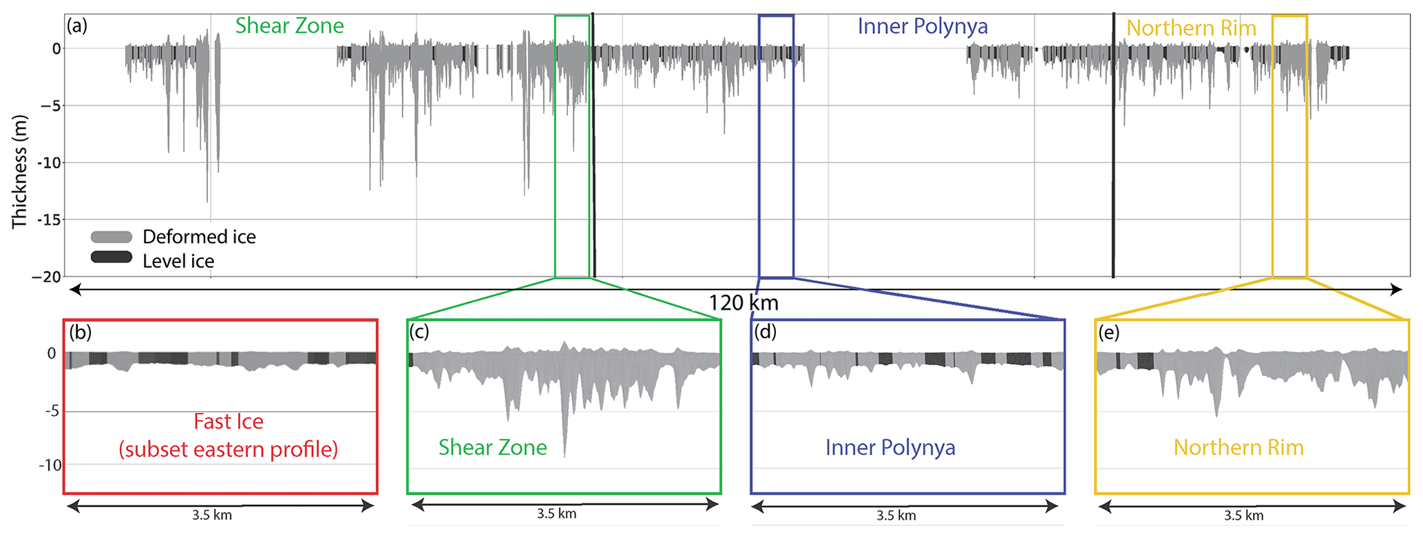
Figure 6Ice thickness profile of the northern profile. The black and gray colors distinguish between level and deformed ice. Four subsets, representative of the four thickness zones, are displayed in (b)–(e). The locations of the subsets (c)–(e) are indicated in (a). The Fast Ice zone is present in the first kilometers off the coast of all profiles but extends only on the eastern profile for more than 8 km (see Fig. 1). Note the different degrees of deformation in the four zones, depicted by the areal fraction of level ice and the total thickness of the ridges. For the eastern and central profiles, see Supplement.
Figure 1 indicates the location of the four zones, and Fig. 6 gives an example of the ice thickness in the zones along the northern AEM profile. ITDs of the same zone but on different profiles resembled each other well. In contrast, the mean thickness and shape of the ITDs of each zone differed strongly from each other. We combined the ice thickness observations of each zone from all profiles and present their ITDs in Fig. 5. The modal thicknesses of the four zones reveal only small differences, which is expected from the uniform thermodynamic growth discussed above (Table 1). However, the ITDs differ strongly in mean thickness, e folding, FWHM, and maximum ice thickness (Table 1, Fig. 5). Since those properties are sensitive to dynamic ice redistribution, we consider them indicative of the different deformation histories of the zones. The ITD of the Fast Ice zone shows the weakest signs of ice thickness redistribution, with the smallest mean thickness and the highest areal fraction of level ice, while the ice in the neighboring Shear Zone shows the strongest signs of deformation with the largest mean, e folding, and FWHM (Table 1). In contrast to all other sections, the Shear Zone lacks a clearly defined peak that could be related to the level ice thickness, which can be associated with the large fraction of deformed ice. In the Shear Zone, the AEM measurements showed ridges with a thickness of up to 20 m (Fig. 1). The ice in the Inner Polynya and the Northern Rim had properties between those two extremes, where the ITD of the Inner Polynya indicates less ice redistribution than the one of the Northern Rim. We obtained more evidence for the inferred differences in deformation by reconstructing the individual deformation histories along the Lagrangian ice drift trajectories.
Table 1Properties of ITDs of different zones of the refrozen polynya and the result of the simple, volume-conserving thickness model (see Sect. 3.3). Mean thickness is shown with standard deviation.
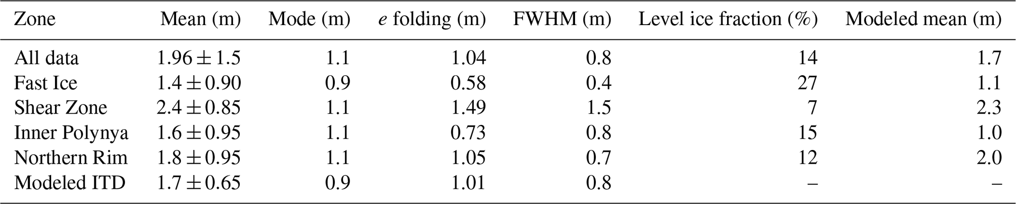
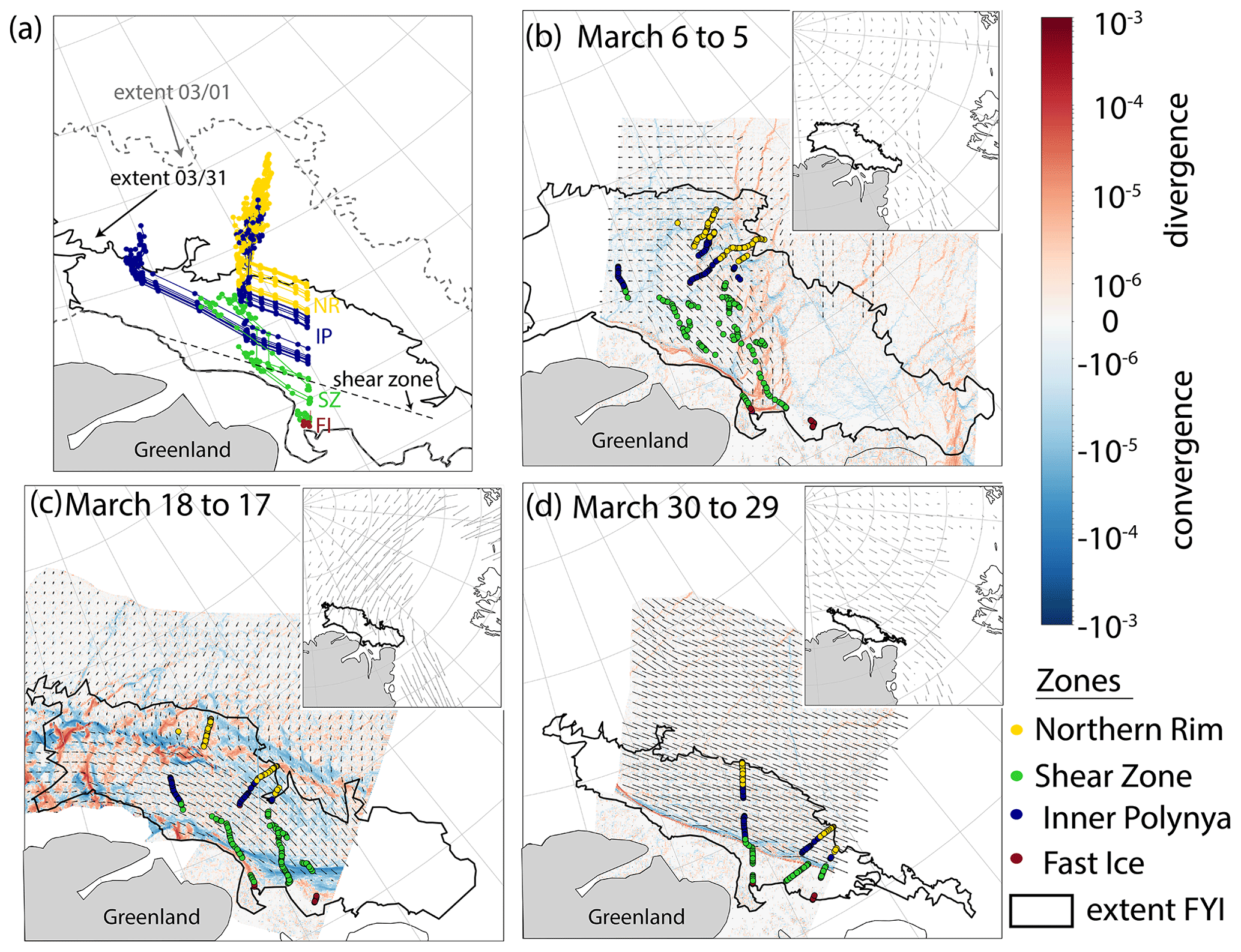
Figure 7Trajectories, drift, and deformation during the three main deformation phases. (a) Example of trajectories initialized on the northern profile. Their colors indicate the zone in which they end. (b, c, d) Snapshots of divergence (red), convergence (blue), and drift (arrows) within the FYI area during the three main deformation phases. The density and length of arrows indicate the magnitude of drift. Colored dots mark the location of the trajectories at the respective time. The insets show the average, large-scale drift of a 48 h period covering the indicated time (arrows, low-resolution drift, OSI SAF, OSI-405-c; see “Data availability” at the end of the text) linked to the local deformation within the FYI.
The dominant direction of the 715 reconstructed trajectories (see Sect. 2.5) was south-southeast, and the total distance traveled by the ice along the trajectories within 1 month varied strongly between 0.3 and 221 km (Figs. 1, 7a). The drift velocity was unsteady, varying between 0 and 45 km d−1. Extracting the deformation along the Lagrangian trajectories provided valuable insights into the different deformation histories and origins of the ice, naturally affecting the ice thickness distributions of the four zones (Fig. 7, video supplement 2). For example, the ice parcels of the Shear Zone experienced divergence in the early deformation phase (Fig. 7b, 3–6 March). During the main deformation phase, convergence along the coast dominated their deformation history (Fig. 7c, 16–20 March). In the late deformation phase, ice in the Shear Zone became immobile and experienced strong shear and convergence. The ice located seaward of a more than 400 km long, dextral shear zone close to the coast (Inner Polynya, Northern Rim) continued to move southward without significant deformation (Fig. 7d, 27–31 March).
In short, we were able to identify four zones across the FYI with clearly differently shaped ITDs and different deformation histories. Since thermodynamic growth was rather uniform, we conclude that the observed spatial thickness variability is fully linked to the deformation history of the ice. In the following section, we will further explore this link on a more quantitative basis.
Relationships between magnitude of deformation and the shape of the ITD
In the previous section, we qualitatively described the relationship between the spatially varying deformation and ice thickness properties. Here, we provide quantitative relationships between divergence and total deformation on the one hand and different ITD properties on the other hand using linear regression (Fig. 8). Since we focus on a period starting on 1 March, we subtracted the thermodynamic thickness of 0.38 m, which was reached on that day, from the mean thickness on 30/31 March. We averaged the deformation along all trajectories separately for each zone to obtain the corresponding mean deformation.
Figure 8 shows that increasing convergence (negative divergence) and total deformation are proportional to increasing mean thickness, e folding, and FWHM. Note that all linear regressions between thickness change and deformation as given in Fig. 8 represent the ice thickness change obtained within 30 d. Like Itkin et al. (2018) and Kwok and Cunningham (2016) we find evidence of a linear relationship between convergence and thickness change (Fig. 8a). Small deviations from this relationship for the Inner Polynya and Fast Ice zones are well within the range of uncertainty indicated by the standard deviation of the convergence. As the Fast Ice zone is much smaller than the Inner Polynya zone, fewer data points were available to compute the means and standard deviations.
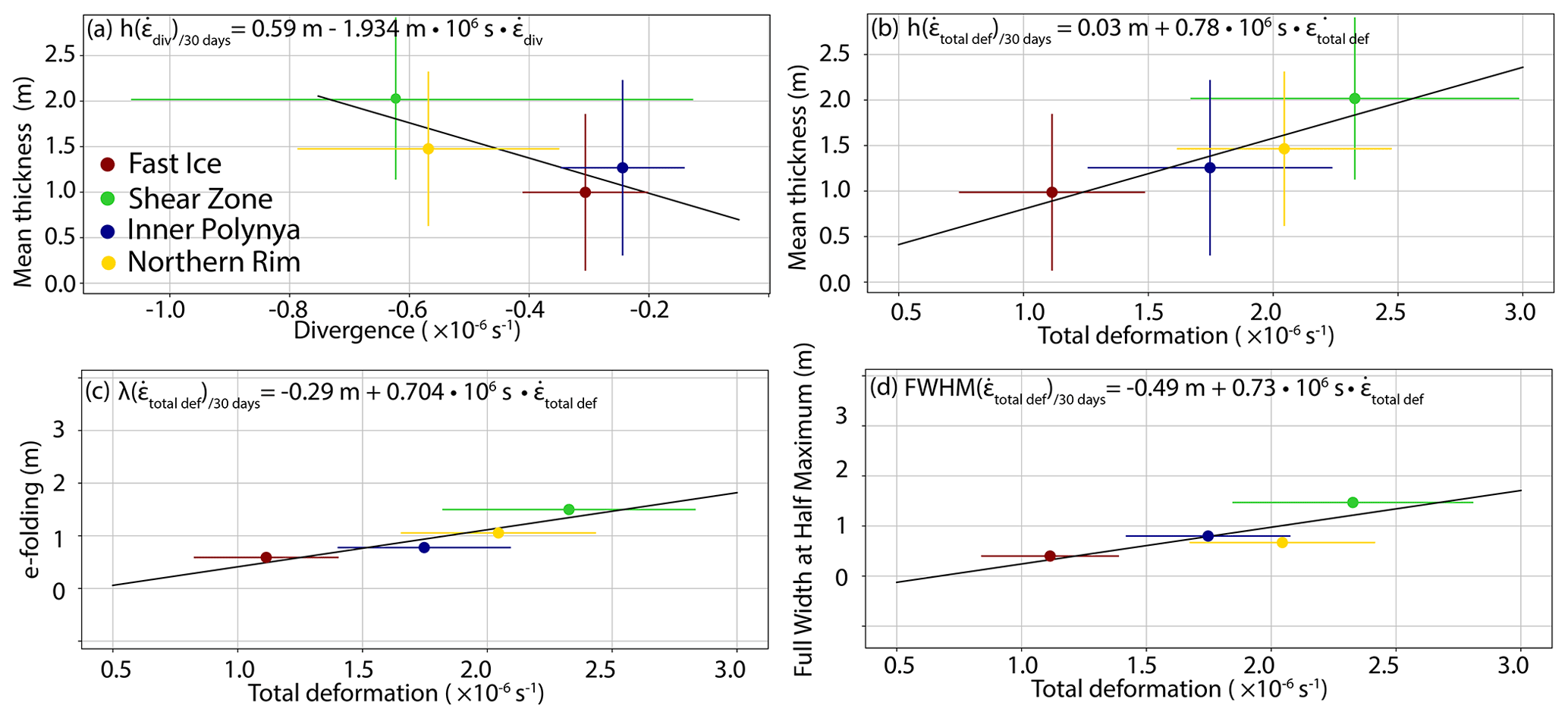
Figure 8Relationship between mean deformation and ITD key parameters in the four polynya zones. If applicable, standard deviations are displayed as error bars. Thickness and mean deformation are given for 1–31 March. We subtracted the thermodynamic thickness of 0.38 m that was reached on 1 March from the mean thickness on 30/31 March. Note that convergence is negative divergence.
3.3 Modeling local thickness variations from high-resolution deformation fields
In the two previous sections, we described the impact of the polynya-wide deformation and its local variations on the thickness distribution. We demonstrated that the area decrease of the closing polynya could directly be used to accurately predict the corresponding ice thickness increase (Sect. 3.1.2). In this section, we present the results of the simple volume-conserving model (Sect. 2.6) that allows us to compute local ice thickness change from high-resolution deformation information. We will evaluate the performance of this simple model by comparing it to the observed average thickness change (Sect. 3.3.1), the observed ITD (Sect. 3.3.2), and the observed spatial thickness variability in the four different zones (Sect. 3.3.3).
3.3.1 Average thickness change
We modeled thickness change along each of the 715 trajectories based on the modeled thermodynamic growth from the MITgcm run and the observed deformation between 1 and 31 March, as described in Sect. 2.6. Figure 4b summarizes the relative contributions of dynamic and thermodynamic growth to the mean thickness. The large standard deviations indicate strong spatial variability among the different trajectories.
In Fig. 4 we marked the deformation phases derived from the time series of area decrease (Sect. 3.1.2). Since the ice was thin in the early deformation phase, the model simulations showed only a weak thickness increase, while the strongest increase in thickness occurred in mid-March. The late deformation phase consisted of both convergent and divergent motion in different regions of the trajectories. On average, divergence dominated, and mean ice thickness decreased during that phase. At the end of the observation period, the simulations (thermodynamic and dynamic, i.e., red and gray curve in Fig. 4a) resulted in a mean total thickness of 1.7 m (blue curve), 11 % smaller than the observed thickness of 1.96 m (orange square). Comparing the simulated thickness with the one derived from the polynya area decrease (black curve, Fig. 4a; Sect. 3.1.2), we note that there is good agreement until 21 March. Only after that date does the area-derived ice thickness increase slightly more rapidly than the simulated thickness, resulting in a thickness difference of 0.26 m. The divergent conditions and ice thickness decrease at the end of the study period between 30 and 31 March is present in both time series (Fig. 4a) and also results in the small amounts of open water in the ITD (Fig. 3).
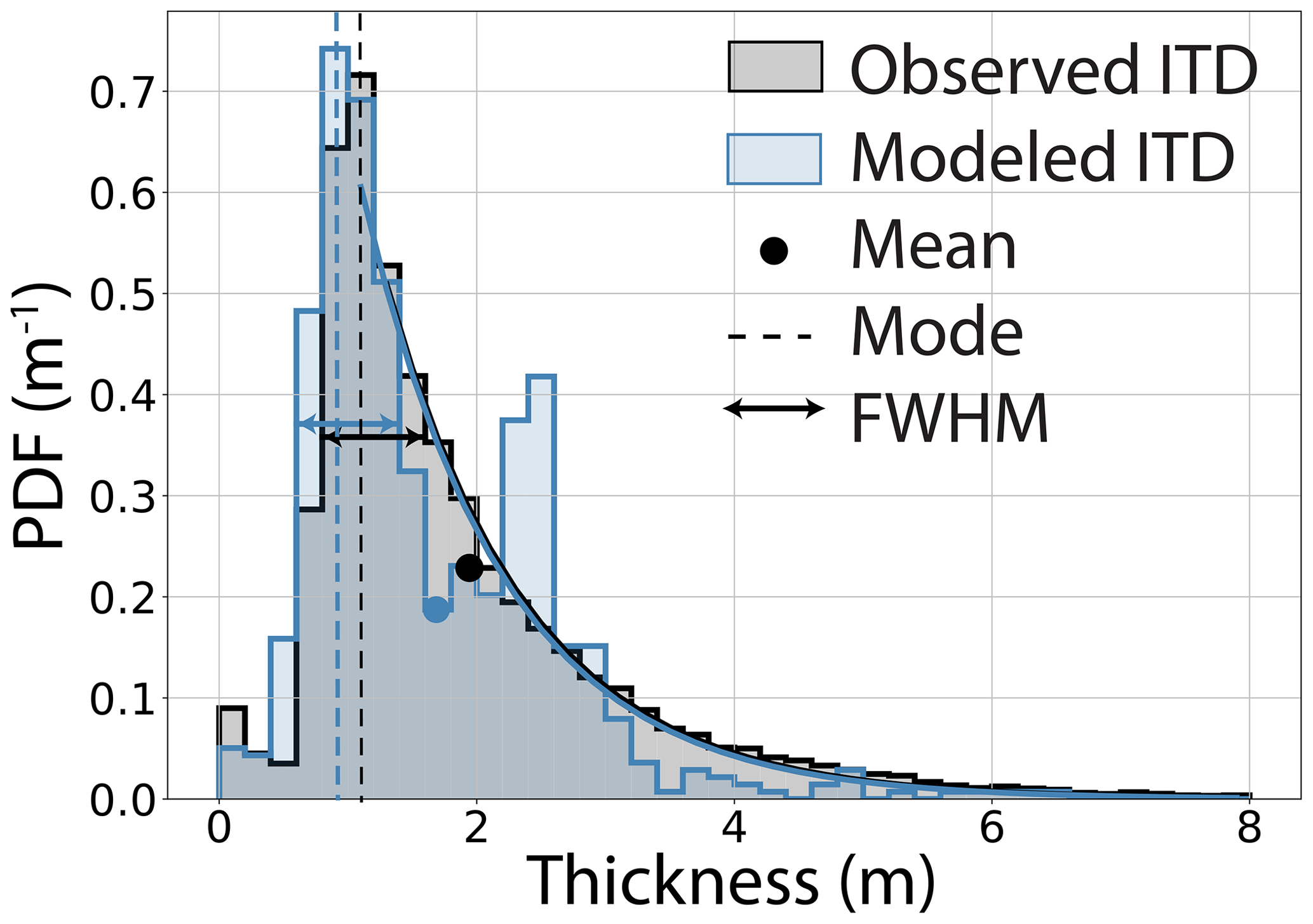
Figure 9Observed and modeled ITD with mean (dot), exponential fit to the tail of the distribution, and FWHM (horizontal bar).
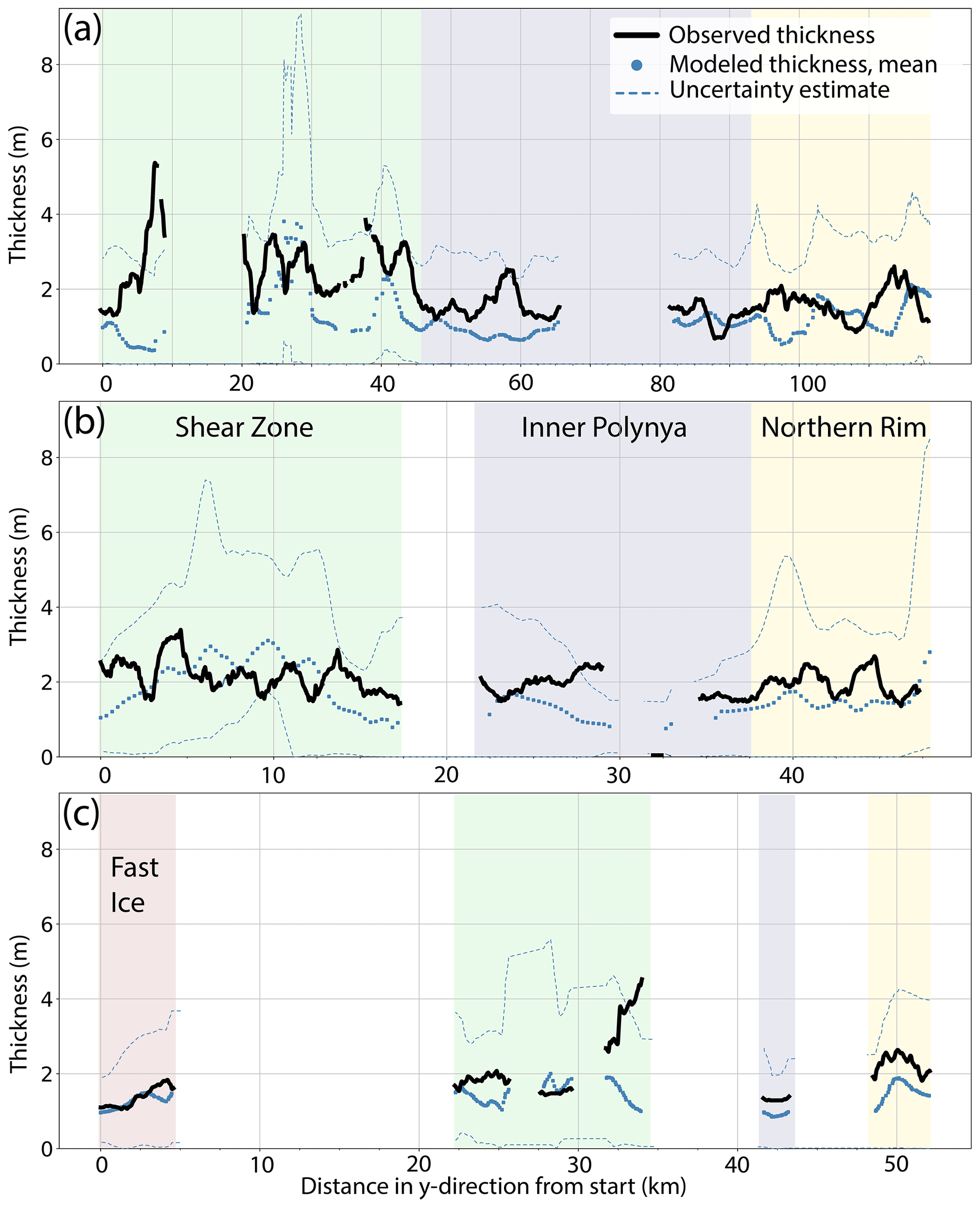
Figure 10Modeled and observed thickness profiles across the FYI from south (left) to north (right) of (a) the northern profile, (b) the central profile, and (c) the eastern profile. The four zones are marked with colors. Modeled mean thicknesses are given with the uncertainty derived from the tracking (Sect. 2.5.1). Note different x-axis scales based on different lengths of profiles (see Fig. 1).
3.3.2 Comparison of modeled and observed ITDs
The ITD of the modeled thicknesses along the 715 trajectories on 30/31 March is shown in Fig. 9, together with the observed ITD. The modeled ITD shows a good resemblance to the observed ITD. Both show a strong, similar mode and a long tail of thick ice that dominates the mean. The mean, mode, e folding, and FWHM are also similar between both ITDs (Table 1). However, the modeled ITD lacks the frequent occurrence of ice thicker than 3 m. Additionally, the modeled ITD possesses a secondary mode at 2.2–2.4 m which is absent in the observations.
3.3.3 Spatial agreement between modeled and observed thickness profiles
Lastly, we compared the modeled and observed thicknesses along the three AEM profiles (Fig. 10). The modeled thickness profiles represent the thickness at the last time step of each trajectory on 30/31 March. For the results shown in Fig. 10, the observed and modeled thicknesses were averaged with a running mean to a resolution of 2.5 km along the profiles. The figure shows that the modeled thicknesses generally reproduce the characteristic variability of the four zones (Table 1). However, they underestimate the observed thickness at most points of the profiles. Considering the uncertainties in the positions of the trajectories and possible errors in the estimation of the deformation parameters, as discussed in Sect. 2, the deviations were expected. Nevertheless, with a better knowledge of the required input parameters, e.g., a smaller accumulated trajectory position error, our method will produce results that reveal a closer match with the observations.
4.1 Dynamic contribution to mean thickness
One of our key results is that after only 1 month of thermodynamic and dynamic thickness growth, the ice thickness in the refrozen polynya had increased from 0.4 to 2 m. Sea ice deformation had contributed on average 50 % and locally up to 90 % to the mean ice thickness. This large contribution of sea ice dynamics is consistent with Kwok and Cunningham (2016), who attributed approximately 42 %–56 % of the seasonal changes in mean regional ice thickness to dynamics in the Canadian Arctic Archipelago. In the light of a future Arctic ice cover which is expected to be thinner and more dynamic than it is now, our results may improve predictions on the impact of sea ice dynamics on future ice thickness changes, especially if stronger and more frequent deformation could partially compensate for the expected increase in sea ice loss. For example, Itkin et al. (2018) concluded that divergence in winter followed by new ice formation is currently responsible for an ice volume increase of 7 % in the sea ice north of Svalbard.
Our results obtained on local scales of a refrozen polynya and over 1 month bridge the spatial and temporal gap between two recent, similar studies of ice deformation and thickness change: the short-term, local-scale study by Itkin et al. (2018) and the long-term, basin-wide study by Kwok and Cunningham (2016). Itkin et al. (2018) observed deformation and ridge formation of a single deformation event with two airborne laser scanning flights a week apart, while Kwok and Cunningham (2016) used CryoSat-2 ice thickness and low-resolution deformation data of several months. Note that the study of Itkin et al. (2018) took place in the pack ice north of Svalbard, while Kwok and Cunningham (2016) studied ice north of the Arctic coasts of the Canadian Arctic Archipelago and Greenland. Both these studies and our own provide evidence for the large contribution of deformation to thickness change at different locations and on different temporal and spatial scales, while also contributing to improved representation of sea ice deformation and thickening in sea ice models.
4.2 The magnitude of deformation shapes the ITD
Our observations provide insights into two key aspects in modeling sea ice dynamics, namely, the mean dynamic thickness change and the effect of deformation on the shape of the ITD, whose accurate representation in models is the subject of current research (e.g., Lipscomb et al., 2007; Ungermann and Losch, 2018).
First, our results showed that mean dynamic thickness change can be approximated as a linear function of convergence (Fig. 8a). This is in good agreement with other observational studies (Itkin et al., 2018; Kwok and Cunningham, 2016) and the redistribution theory (Thorndike et al., 1975; Hibler, 1979) that forms the basis for sea ice dynamics in most models. We normalized the slope and intercept of the least-squares fit (see Fig. 8a) to 1 d. For a more intuitive interpretation, we give div(v) in units of per day (d−1). From this we can compare the least-squares fit with Eq. (4) (Sect. 2.6):
The thermodynamic growth term (Δhth,t) of 0.0199 m d−1 results in 0.59 m of ice growth if integrated over 30 d (see intercept, Fig. 8a). The 0.59 m corresponds reasonably well to the observed thermodynamic growth of 0.49 m between 1 and 30/31 March.
The redistribution theory (Thorndike, 1992; Hibler, 1979) suggests that the slope of the dynamic growth term (div(v) h) is given by the thickness of the ice participating in ice compression (h). Since we observed the integrated effect of a series of deformation events during 1 month, h represents the weighted average of ice of varying thickness that contributed to ridging during that time. Since most of the dynamic thickness change is associated with the main deformation phase, we approximate h with the thickness of the ice that participated during the main deformation phase between 16–20 March. Indeed, the slope of 0.746 m agrees well with the mean thickness of 0.75 m at the beginning of this phase on 16 March (see Fig. 4). Differences between our observations and the coefficients as suggested by the redistribution theory in Eq. (7) are within the uncertainties in the linear regression.
Second, our results suggest that the e folding of the ITD is proportional to the deformation rate (Fig. 8c). The e folding is defined in the redistribution function that describes how the ice participating in deformation is distributed over the different thickness categories (Thorndike et al., 1975). Previous observational studies have shown that an exponential function with a constant, negative exponent of between λ=3 and λ=6 approximates well the tail of ITDs derived from ice draft thicker than 5 m (e.g., Vinje et al., 1998; Amundrud et al., 2004). Sea ice models based on Lipscomb et al. (2007) use an exponential ridge redistribution function with a variable e folding that depends on ice thickness rather than on the deformation rate, with , where hi refers to the thickness of the ice that was ridged and μ is a tunable parameter that is used to improve the fit between model and observations.
We test whether different ice thicknesses as suggested by Lipscomb et al. (2007), rather than different deformation rates as found here, can explain the range of e foldings between 0.6 and 1.5 m as was observed by us. Following Lipscomb et al. (2007) we assume that the relationship between e folding and thickness in the ridge redistribution function defined for a single ridging event is passed on during a series of deformation events, leading to the final ITD. Granted that the contribution shaping the tail of the ITD comes mostly from the undeformed, thermodynamically grown ice, i.e., from ice with a thickness between 0.49 and 0.86 m, the e folding could only vary by a factor of , assuming that the tunable parameter μ is constant. However, our observed range of e-folding values correspond to a factor of 2.5; i.e., the relation to thickness alone cannot explain the variability.
Based on the good linear fit (Fig. 8c), we attribute the large range in the e folding to the magnitude of the deformation rate in agreement with Rabenstein et al. (2010), who related the differences in ITD shape in the Arctic Transpolar Drift to varying amount of convergence. Hence, we suggest choosing the parameter μ as a function of the deformation rate. Since Ungermann and Losch (2018) showed in a sensitivity study with the MITgcm that μ is an important parameter in shaping the modeled ITD, we expect this to improve the fit between modeled and observed ITDs.
We identified two processes that change the e folding and potentially link it to the deformation rate.
-
Ridge formation models from Hopkins (1998) and Hopkins et al. (1991, 1999) showed that ridges first reach a maximum dynamic thickness and then continue to grow laterally. This lateral growth widens the ridge and therefore increases the relative occurrence of deformed ice with the maximum dynamic thickness, reducing the e folding. When a ridge begins to form, the balance of the force needed to push ice farther up or down and the force needed to fracture the ice is decisive for its redistribution. In this process, ice thickness and friction plays a major role. When the maximum dynamic thickness is reached, the ridge grows laterally in proportion to the ongoing deformation. In this stage, larger deformation rates result in wider ridges with the maximum thickness and smaller e folding. Applying the maximum keel draft criterion of Amundrud et al. (2004), we identified several ridges in the measured thickness profiles in the Shear Zone that had reached the maximum ice thickness. However, the relationship between e folding and the deformation rate might only be applicable in regions that experience strong deformation, e.g., coastal regions. Hopkins (1998) and Amundrud et al. (2004) pointed out that ridges in the central Arctic rarely reach the maximum thickness as the critical stresses often do not last long enough to complete the ridge-building process.
-
Rafting leads to a different e folding than ridging. Riding distributes more ice into a few thicker ice thickness categories, while rafting leads to deformed ice with a relatively uniform thickness of only double the original one. If the occurrence of rafting and ridging depends on the magnitude of deformation, this could establish a link between e folding and the deformation rate. Hopkins et al. (1999) identified that the relative likelihood of rafting increases with increasing homogeneity of the ice floes. Hence, regions like the Fast Ice zone that only experienced little deformation and with the ice still of relatively uniform thickness might have a higher portion of rafted ice and thus a different e folding than regions that experienced more ridging. Consequently, the e folding could also depend on the initial composition of thin and thick ice and on the deformation history.
Lastly, we acknowledge other aspects: the creation of rubble fields, hummocks, or the ratio of shear to convergence could influence the e folding. The shear-to-convergence ratio varied among the four zones in the polynya, but we could not draw any conclusion due to too few data points. Since we do not have more frequent thickness observations during the closing of the polynya, we can only evaluate the impact of deformation integrated over 30 d. Therefore, we also overlook information about potentially contrasting effects like, e.g., ridge consolidation and collapse.
4.3 Modeled vs. observed thickness – limitations of the model
Based on a simple volume-conserving model, we derived thickness change along ice drift trajectories and calculated ITDs from the final thickness at the end of each trajectory.
Kwok (2002) showed that SAR-derived deformation could be used for reasonable bulk estimates of dynamic thickness change of the seasonal ice cover using RGPS drift and deformation. Our comparison between the modeled and observed ice thickness with much higher spatial and temporal resolutions corroborates this. We note that SAR-derived deformation can even predict local spatial variability.
The modeled ITD resembles the observed one in the typical, skewed shape with a dominant central mode and a long tail of thicker ice (Sect. 3.3, Fig. 9). We obtained the modeled ITD from a spatial resolution of 1.4 km. ITDs based on radar altimetry data, e.g., CryoSat-2 ITDs of, e.g., Kwok (2015), were derived from measurements averaged over similar spatial scales, i.e., an altimeter footprint of approximately 0.31 km by 1.67 km in the along- and across-track direction, respectively. Therefore, the resolution and character of the ITDs obtained with our volume-conserving model and ITDs derived from strongly averaged radar altimetry data are comparable.
Our modeled ITD agrees well with the observations in the thinner thickness categories. However, it shows a second mode at 2.2–2.4 m (Fig. 9) that was not observed, and it underestimates the amount of ice thicker than 3.5 m. Because of the size of one grid cell in our model, the maximum thickness of single ridges cannot be simulated. The reason for the second mode is that ice with a thickness of 0.75–1.2 m was advected into many grid cells during the main deformation phase, doubling their thickness to 1.5–2.4 m (Fig. 4). Smaller grid cells will lead to more realistic ice thickness distributions by considering the effect of ridging in more detail.
Apart from those differences in the shape of the ITD, we have found that the modeled mean ice thicknesses were generally smaller than the observed ones (Table 1). As the agreement between modeled and observed thermodynamically grown ice was quite good, we attribute the general underestimation of mean thicknesses to problems in the modeling of the dynamic contribution. There are two main shortcomings of the model:
First, our model does not account for the high macro-porosity of unconsolidated FYI ridge keels, which leads to an underestimation of the thickness. Numerous studies have shown that mean ridge porosities amount to 11 %–22 % (Kharitonov and Borodkin, 2020; Kharitonov, 2019a, b; Strub-Klein and Sudom, 2012), with the largest range between 11 % and 45 % for old FYI ridges and newly formed FYI ridges, respectively (Ervik et al., 2018; Høyland, 2007). If we assume that the fraction of 86 % of deformed ice in all observations had a porosity of 11 %–22 %, the mean modeled thickness will increase by 0.1–0.3 m, to 1.8–2 m. In the context of porosity, we also discuss the uncertainties in the EM ice thickness measurements. While the accuracy of EM measurements is ± 0.1 m over level ice, EM measurements typically underestimate the maximum thickness of pressure ridges (Haas et al., 2009) due to (1) porosity and (2) footprint averaging. However, despite this shortcoming, most AEM thicknesses obtained here were still larger than the modeled thicknesses. This provides evidence that the mean AEM ice thickness estimates over length scales of 1–2 km are not the main source for the observed underestimation.
Second, in the simple, volume-conserving model, the thermodynamic growth was modeled based on the growth of an undeformed layer of ice, regardless of the actual mean thickness of each grid cell. Hence, the model overestimates thermodynamic growth in all cells that experienced strong convergence and were, therefore, thicker than the thermodynamic thickness. At the same time, our approach underestimates ice growth in all cells that experienced divergence because thermodynamic growth is stronger in leads than in adjacent consolidated ice. We carried out a sensitivity study to estimate the impact of unaccounted for new ice formation in leads. If there was divergence, we replaced the ice leaving the grid cell with new ice of a thickness that could form within 1 d. Integrated over 30 d and all profiles, this resulted in an additional 0.3 m of ice, i.e., a mean thickness of 2 m. Since the dominating deformation type in this study was convergence and shear, this effect is less important than in a different deformation regime. We suggest coupling the deformation history retrieved from SAR analysis with a fully developed sea ice model that considers those interdependencies in future work. For example, the single-column model Icepack includes full solutions for thermodynamic growth and melting, as well as mechanical redistribution due to ridging (see CICE Consortium Icepack, 2020). SAR-derived deformation rates can be used to force the mechanical redistribution of ice in the Icepack model.
Both those shortcomings can explain the observed differences in the mean thicknesses. However, there are additional reasons for deviations of observed and modeled thickness briefly discussed below.
-
The daily imaging of the polynya by SAR images cannot account for deformation caused by tides. Tides and inertial motion can cause recurrent opening and closing with associated sub-daily new ice formation and subsequent deformation. These processes can contribute 10 %–20 % of the Arctic-wide seasonal ice growth (Kwok et al., 2003; Heil and Hibler, 2002; Hutchings and Hibler, 2008). Due to the polynya's location across the continental slope, tidal currents in this region exceed the ones in the central Arctic that are on the order of 0.5–1 cm s−1 (Baumann et al., 2020). In the polynya region over the continental slope (83.2∘ N, 22.9∘ W) the Oregon State University tide model (Egbert and Erofeeva, 2002) states tidal currents of up to 5–6 cm s−1, and oceanographic measurements under the fast ice close to Station Nord indicated semi-diurnal tidal currents on the order of 2 cm s−1 (Kirillov et al., 2017). Assuming a contribution of tides to sea ice formation of at least a similar order to that in the central Arctic, tides could have contributed, in our case, an additional new ice growth of 0.14–0.28 m.
-
Single early deformation processes before 1 March might already have created an inhomogeneous ice thickness field in contrast to our assumed, initial, uniform thickness. Since we did not observe a decrease in the total polynya area between 25 February and 1 March, ice thickness variations in this period could only be explained by localized effects.
-
Even the consideration of the uncertainties in the deformation parameters and in the positions of trajectories cannot explain all deviations between modeled and observed thickness (Fig. 10). Due to deformation's highly localized nature in time and space, the true deformation rates might be larger than the calculated, averaged ones. For example, during the main deformation phase, Fig. 4a shows that the area-derived thickness (black line) indicates more thickness increase than the thickness derived from the deformation along the trajectories (blue line). A potential underestimation of the deformation rate during this strongest deformation event could explain the thinner modeled ice thickness.
-
We did not consider additional opening and closing of ice due to shear on subgrid scales that can be observed in similar situations (e.g., Stern et al., 1995; Kwok and Cunningham, 2016). However, the effects of divergence and convergence on mean thickness compensate for each other on a subgrid scale in the simple, volume-conserving model, apart from the impact of divergence on new ice formation (see above, main sources of uncertainty).
An unusual latent heat polynya with a size of >65 000 km2 occurred in late winter 2018 at the coast of North Greenland and provided us with a unique opportunity to observe a natural but well-constrained, large-scale ice deformation experiment. While the open water refroze quickly due to low air temperatures, convergent ice motion deformed the newly formed ice. One month after the maximum extent of the polynya was observed, the area had halved, accompanied by a strong impact on the ice thickness distribution. In our case study, we analyzed thickness profiles from airborne electromagnetic (AEM) measurements and their relationship to deformation obtained from high-resolution synthetic-aperture radar (SAR) satellite images. We reconstructed Lagrangian trajectories of the surveyed ice parcels backward in time to retrieve the deformation history. The objective was to link the magnitude of deformation to the ice thickness distributions and to show that deformation derived from SAR images can be used to derive dynamic thickness change of the region.
This study provides evidence of the high relevance of deformation dynamics in creating and maintaining a thick ice cover. In the refrozen polynya, sea ice deformation contributed on average 50 % and locally up to 90 % to the mean thickness. Within 1 month, the dynamic processes re-established an ice cover with a mean thickness of 1.96 m, almost as thick as the surrounding multi-year ice, which had a mean thickness of 2.1 m (results not shown here).
In the view of a changing Arctic with increasing fractions of thin ice, increased ice drift speed, and a higher frequency of deformation events, accurate representation of sea ice deformation in models is crucial for predictions of future sea ice thickness and extent. Our observations reveal new insights into the link between deformation and the redistribution of ice, which determines the shape of the ice thickness distribution (ITD). We provide quantitative evidence that the deformation magnitude impacts the e folding of the ITD. These findings can be used for further improving the representation of ITDs in sea ice models, e.g., by constraining the parameterization of the ridge redistribution function. Further, we found that mean dynamic thickness change is a linear function of convergence in close agreement with the redistribution theory (Thorndike et al., 1975; Hibler, 1979) and previous observational studies (Itkin et al., 2018; Kwok and Cunningham, 2016).
We developed a simple volume-conserving model to derive dynamic thickness change from deformation fields with a spatial resolution of 1.4 km obtained from SAR satellite imagery. The modeled mean thicknesses were smaller than AEM thickness observations, but they agree within the limits of the main uncertainties due to ridge porosity and omitted new ice formation in leads formed by divergence.
The volume-conserving model allowed us to reconstruct an ITD that resembled the ITD obtained from the AEM thickness observations. They both have the typical skewed shape with a dominant central mode and a long tail of thicker ice. However, we note that without a redistribution scheme, the thickest ice of the ITD cannot be realistically modeled.
For future work, we suggest coupling the deformation history retrieved from SAR analysis with a fully developed sea ice model that takes drift and deformation as forcing and calculates dynamics and thermodynamics for several thickness categories, e.g., Icepack (CICE Consortium Icepack, 2020). Considering the increasing availability of SAR data in the polar regions, this opens up the possibility of deriving dynamic thickness change and ITDs for many regions of the Arctic and Antarctic sea ice cover.
Sentinel-1 scenes are available from the Copernicus Open Access Hub (https://scihub.copernicus.eu/dhus/#/home, ESA, 2020) and can be processed with the open-source software SNAP (https://step.esa.int/main/toolboxes/snap/, SNAP, 2020). AEM thickness data are available via https://doi.pangaea.de/10.1594/PANGAEA.927445 (Rohde et al., 2021a) and https://doi.pangaea.de/10.1594/PANGAEA.927448 (Rohde et al., 2021b). High-resolution drift and deformation data are available via https://doi.pangaea.de/10.1594/PANGAEA.927451 (von Albedyll et al., 2021). The low-resolution sea ice drift product (OSI-405-c) of the EUMETSAT Ocean and Sea Ice Satellite Application Facility (OSI SAF) used in Fig. 7 is available via http://osisaf.met.no/p/ice/lr_ice_drift.html (EUMETSAT OSI SAF, 2020). Details on the motion-tracking methodology are published in Lavergne et al. (2010). Low-resolution, monthly sea ice drift products used in Fig. 1 are monthly mean sea ice motion vectors derived from Tschudi et al. (2019; https://doi.org/10.5067/INAWUWO7QH7B) and were provided in NetCDF format (file version fv0.01) by the Integrated Climate Data Center (ICDC; https://icdc.cen.uni-hamburg.de/, last access: 11 May 2020), University of Hamburg, Hamburg, Germany. Snow estimates were obtained from Operation IceBridge (2016, updated 2019; https://doi.org/10.5067/GRIXZ91DE0L9).
Video supplement 1 (available at https://doi.org/10.5446/50650) is a time series of SAR images of the refrozen polynya from 1 to 31 March 2018. The outlines of the polynya (red) are manually drawn based on the backscatter contrast. Video supplement 2 (available at https://doi.org/10.5446/49540) shows a time series of divergence and shear in the refrozen polynya from 1 to 31 March 2018. Dots display the location of selected trajectories on the respective dates specified in the title. Lines show the traveled distance within the last time step. Arrows indicate sea ice drift. The colors show the magnitude of divergence (left) and shear (right). The video supplement is made available via TIB AV-Portal.
The supplement related to this article is available online at: https://doi.org/10.5194/tc-15-2167-2021-supplement.
LvA carried out the analysis, processed the deformation data, and wrote the manuscript. All authors contributed to the discussion and provided input during the concept phase and the writing process.
Christian Haas is a member of the editorial board of The Cryosphere. All other authors declare that they have no conflict of interest.
We thank Martin Losch for fruitful discussions on the content of this paper and for helping set up the MITgcm model runs. Thomas Hollands supported us with the tracking algorithm. Nils Hutter provided initial oceanographic data sets for the model runs. Stefan Hendricks and Jan Rohde were involved in the field campaign and processed the AEM data. Thomas Krumpen and Florent Birrien provided guidance on the thermodynamic growth in the polynya. Conor Murray gave valuable feedback on copy-editing. This work contains modified Copernicus Sentinel data (2019), and snow thickness data used in this study were acquired by NASA's Operation IceBridge. We acknowledge EUMETSAT Ocean and Sea Ice Satellite Application Facility (OSI SAF; http://www.osi-saf.org/, last access: 11 May 2020) for the low-resolution sea ice drift products. The Department of Environmental Science, Aarhus University, is acknowledged for providing data from the Villum Research Station in North Greenland. We thank the editor, Jennifer Hutchings, for editing the paper. We thank Amélie Bouchat and the anonymous reviewer for reviewing our paper. Their comments greatly helped to improve the content, structure, and clarity of the paper.
This research was funded by the Alfred Wegener Institute Helmholtz Centre for Polar and Marine Research (AWI), through its research program “Polar regions And Coasts in the changing Earth System”, Topic 1.4 “Arctic sea ice and its interaction with ocean and ecosystems”, and by the Deutsche Forschungsgemeinschaft (DFG) through
the International Research Training Group (IRTG) ArcTrain (GRK1904).
The article processing charges for this open-access publication were covered by the Alfred Wegener Institute, Helmholtz Centre for Polar and Marine Research (AWI).
This paper was edited by Jennifer Hutchings and reviewed by Amélie Bouchat and one anonymous referee.
Amundrud, T. L., Melling, H., and Ingram, R. G.: Geometrical constraints on the evolution of ridged sea ice, J. Geophys. Res., 109, C06005, https://doi.org/10.1029/2003jc002251, 2004. a, b, c
Baumann, T. M., Polyakov, I. V., Padman, L., Danielson, S., Fer, I., Janout, M., Williams, W., and Pnyushkov, A. V.: Arctic tidal current atlas, Scientific Data, 7, 275, https://doi.org/10.1038/s41597-020-00578-z, 2020. a
CICE Consortium Icepack: Icepack version 1.1.0, Zenodo [code], https://doi.org/10.5281/zenodo.1213462, 2020. a, b
Dierking, W., Stern, H. L., and Hutchings, J. K.: Estimating statistical errors in retrievals of ice velocity and deformation parameters from satellite images and buoy arrays, The Cryosphere, 14, 2999–3016, https://doi.org/10.5194/tc-14-2999-2020, 2020. a
Duncan, K., Farrell, S. L., Hutchings, J., and Richter-Menge, J.: Late Winter Observations of Sea Ice Pressure Ridge Sail Height, IEEE Geosci. Remote S., 1–5, https://doi.org/10.1109/lgrs.2020.3004724, 2020. a
Egbert, G. D. and Erofeeva, S. Y.: Efficient Inverse Modeling of Barotropic Ocean Tides, J. Atmos. Ocean. Tech., 19, 183–204, https://doi.org/10.1175/1520-0426(2002)019<0183:eimobo>2.0.co;2, 2002. a
Ervik, Å., Høyland, K. V., Shestov, A., and Nord, T. S.: On the decay of first-year ice ridges: Measurements and evolution of rubble macroporosity, ridge drilling resistance and consolidated layer strength, Cold Reg. Sci. Technol., 151, 196–207, https://doi.org/10.1016/j.coldregions.2018.03.024, 2018. a
ESA: Copernicus Open Access Hub, https://scihub.copernicus.eu/dhus/#/home, last access: 14 January 2020. a
EUMETSAT Ocean and Sea Ice Satellite Application Facility (OSI SAF): Low resolution sea ice drift product, http://osisaf.met.no/p/ice/lr_ice_drift.html, last access: 11 May 2020. a
Flato, G. M. and Hibler, W. D.: Ridging and strength in modeling the thickness distribution of Arctic sea ice, J. Geophys. Res., 100, 18611, https://doi.org/10.1029/95jc02091, 1995. a
Griebel, J. and Dierking, W.: Impact of Sea Ice Drift Retrieval Errors, Discretization and Grid Type on Calculations of Ice Deformation, Remote Sensing, 10, 393, https://doi.org/10.3390/rs10030393, 2018. a, b
Haas, C., Gerland, S., Eicken, H., and Miller, H.: Comparison of sea-ice thickness measurements under summer and winter conditions in the Arctic using a small electromagnetic induction device, Geophysics, 62, 749–757, https://doi.org/10.1190/1.1444184, 1997. a
Haas, C., Hendricks, S., and Doble, M.: Comparison of the Sea-ice thickness distribution in the Lincoln Sea and adjacent Arctic Ocean in 2004 and 2005, Ann. Glaciol., 44, 247–252, https://doi.org/10.3189/172756406781811781, 2006. a
Haas, C., Pfaffling, A., Hendricks, S., Rabenstein, L., Etienne, J.-L., and Rigor, I.: Reduced ice thickness in Arctic Transpolar Drift favors rapid ice retreat, Geophys. Res. Lett., 35, L17501, https://doi.org/10.1029/2008GL034457, 2008. a, b
Haas, C., Lobach, J., Hendricks, S., Rabenstein, L., and Pfaffling, A.: Helicopter-borne measurements of sea ice thickness, using a small and lightweight, digital EM system, J. Appl. Geophys., 67, 234–241, https://doi.org/10.1016/j.jappgeo.2008.05.005, 2009. a, b, c, d
Heil, P. and Hibler, W. D.: Modeling the High-Frequency Component of Arctic Sea Ice Drift and Deformation, J. Phys. Oceanogr., 32, 3039–3057, https://doi.org/10.1175/1520-0485(2002)032<3039:mthfco>2.0.co;2, 2002. a
Hendricks, S.: Validierung von altimetrischen Meereisdickenmessungen mit einem helikopter-basierten elektromagnetischen Induktionsverfahren, Ph.D. thesis, Universität Bremen, available at: https://epic.awi.de/id/eprint/20890/1/Hen2009b.pdf (last access: 8 May 2020), 2009. a
Hibler, W. D.: A dynamic thermodynamic sea ice model, J. Phys. Oceanogr., 9, 815–846, 1979. a, b, c, d, e, f
Hollands, T. and Dierking, W.: Performance of a multiscale correlation algorithm for the estimation of sea-ice drift from SAR images: initial results, Ann. Glaciol., 52, 311–317, https://doi.org/10.3189/172756411795931462, 2011. a, b, c
Hollands, T., Linow, S., and Dierking, W.: Reliability Measures for Sea Ice Motion Retrieval From Synthetic Aperture Radar Images, IEEE J. Sel. Top. Appl., 8, 67–75, https://doi.org/10.1109/jstars.2014.2340572, 2015. a
Hopkins, M. A.: Four stages of pressure ridging, J. Geophys. Res.-Oceans, 103, 21883–21891, https://doi.org/10.1029/98jc01257, 1998. a, b
Hopkins, M. A., Hibler, W. D., and Flato, G. M.: On the numerical simulation of the sea ice ridging process, J. Geophys. Res., 96, 4809, https://doi.org/10.1029/90jc02375, 1991. a
Hopkins, M. A., Tuhkuri, J., and Lensu, M.: Rafting and ridging of thin ice sheets, J. Geophys. Res.-Oceans, 104, 13605–13613, https://doi.org/10.1029/1999jc900031, 1999. a, b
Høyland, K. V.: Morphology and small-scale strength of ridges in the North-western Barents Sea, Cold Reg. Sci. Technol., 48, 169–187, https://doi.org/10.1016/j.coldregions.2007.01.006, 2007. a
Hutchings, J. K. and Hibler, W. D.: Small-scale sea ice deformation in the Beaufort Sea seasonal ice zone, J. Geophys. Res., 113, C08032, https://doi.org/10.1029/2006JC003971, 2008. a
Itkin, P., Spreen, G., Hvidegaard, S. M., Skourup, H., Wilkinson, J., Gerland, S., and Granskog, M. A.: Contribution of Deformation to Sea Ice Mass Balance: A Case Study From an N-ICE2015 Storm, Geophys. Res. Lett., 45, 789–796, https://doi.org/10.1002/2017gl076056, 2018. a, b, c, d, e, f, g, h, i, j
Kharitonov, V. V.: Ice ridges in the Shokalsky Strait, the Severnaya Zemlya Archipelago, Earth's Cryosphere, XXIII, https://doi.org/10.21782/ec2541-9994-2019-3(43-50), 2019a. a
Kharitonov, V. V.: Ice ridges in landfast ice of Shokal'skogo Strait, Geography, Environment, Sustainability, 12, 16–26, https://doi.org/10.24057/2071-9388-2019-43, 2019b. a
Kharitonov, V. V. and Borodkin, V. A.: On the results of studying ice ridges in the Shokal'skogo Strait, part I: Morphology and physical parameters in-situ, Cold Reg. Sci. Technol., 174, 103041, https://doi.org/10.1016/j.coldregions.2020.103041, 2020. a
King, J., Howell, S., Derksen, C., Rutter, N., Toose, P., Beckers, J. F., Haas, C., Kurtz, N., and Richter-Menge, J.: Evaluation of Operation IceBridge quick-look snow depth estimates on sea ice, Geophys. Res. Lett., 42, 9302–9310, https://doi.org/10.1002/2015gl066389, 2015. a
Kirillov, S., Dmitrenko, I., Rysgaard, S., Babb, D., Toudal Pedersen, L., Ehn, J., Bendtsen, J., and Barber, D.: Storm-induced water dynamics and thermohaline structure at the tidewater Flade Isblink Glacier outlet to the Wandel Sea (NE Greenland), Ocean Sci., 13, 947–959, https://doi.org/10.5194/os-13-947-2017, 2017. a
Kwok, R.: Seasonal ice area and volume production of the Arctic Ocean: November 1996 through April 1997, J. Geophys. Res., 107, 8038, https://doi.org/10.1029/2000JC000469, 2002. a, b
Kwok, R.: Sea ice convergence along the Arctic coasts of Greenland and the Canadian Arctic Archipelago: Variability and extremes (1992–2014), Geophys. Res. Lett., 42, 7598–7605, https://doi.org/10.1002/2015gl065462, 2015. a, b
Kwok, R.: Arctic sea ice thickness, volume, and multiyear ice coverage: losses and coupled variability (1958–2018), Enviro. Res. Lett., 13, 105005, https://doi.org/10.1088/1748-9326/aae3ec, 2018. a
Kwok, R. and Cunningham, G. F.: Contributions of growth and deformation to monthly variability in sea ice thickness north of the coasts of Greenland and the Canadian Arctic Archipelago, Geophys. Res. Lett., 43, 8097–8105, https://doi.org/10.1002/2016gl069333, 2016. a, b, c, d, e, f, g, h, i, j
Kwok, R., Cunningham, G. F., and Hibler, W. D.: Sub-daily sea ice motion and deformation from RADARSAT observations, Geophys. Res. Lett., 30, 2218, https://doi.org/10.1029/2003gl018723, 2003. a, b
Kwok, R., Hunke, E. C., Maslowski, W., Menemenlis, D., and Zhang, J.: Variability of sea ice simulations assessed with RGPS kinematics, J. Geophys. Res., 113, C11012, https://doi.org/10.1029/2008jc004783, 2008. a
Lavergne, T., Eastwood, S., Teffah, Z., Schyberg, H., and Breivik, L.-A.: Sea ice motion from low-resolution satellite sensors: An alternative method and its validation in the Arctic, J. Geophys. Res., 115, C10032, https://doi.org/10.1029/2009jc005958, 2010. a
Lindsay, R. and Schweiger, A.: Arctic sea ice thickness loss determined using subsurface, aircraft, and satellite observations, The Cryosphere, 9, 269–283, https://doi.org/10.5194/tc-9-269-2015, 2015. a
Lindsay, R. W. and Stern, H. L.: The RADARSAT Geophysical Processor System: Quality of Sea Ice Trajectory and Deformation Estimates, J. Atmos. Ocean. Tech., 20, 1333–1347, https://doi.org/10.1175/1520-0426(2003)020<1333:TRGPSQ>2.0.CO;2, 2003. a
Lipscomb, W. H., Hunke, E. C., Maslowski, W., and Jakacki, J.: Ridging, strength, and stability in high-resolution sea ice models, J. Geophys. Res., 112, C03S91, https://doi.org/10.1029/2005JC003355, 2007. a, b, c, d, e, f
Losch, M., Menemenlis, D., Campin, J.-M., Heimbach, P., and Hill, C.: On the formulation of sea-ice models. Part 1: Effects of different solver implementations and parameterizations, Ocean Modelling, 33, 129–144, https://doi.org/10.1016/j.ocemod.2009.12.008, 2010. a
Ludwig, V., Spreen, G., Haas, C., Istomina, L., Kauker, F., and Murashkin, D.: The 2018 North Greenland polynya observed by a newly introduced merged optical and passive microwave sea-ice concentration dataset, The Cryosphere, 13, 2051–2073, https://doi.org/10.5194/tc-13-2051-2019, 2019. a, b, c, d, e
Maykut, G. A.: The Surface Heat and Mass Balance, Springer US, Boston, MA, 395–463, https://doi.org/10.1007/978-1-4899-5352-0_6, 1986. a, b
Menemenlis, D., Hill, C., Adcrocft, A., Campin, J.-M., Cheng, B., Ciotti, B., Fukumori, I., Heimbach, P., Henze, C., Köhl, A., Lee, T., Stammer, D., Taft, J., and Zhang, J.: NASA supercomputer improves prospects for ocean climate research, Eos, Transactions American Geophysical Union, 86, 89–96, https://doi.org/10.1029/2005eo090002, 2005. a
Moore, G. W. K., Schweiger, A., Zhang, J., and Steele, M.: What Caused the Remarkable February 2018 North Greenland Polynya?, Geophys. Res. Lett., 45, 13342–13350, https://doi.org/10.1029/2018gl080902, 2018. a, b, c, d
Nghiem, S. V., Rigor, I. G., Perovich, D. K., Clemente-Colón, P., Weatherly, J. W., and Neumann, G.: Rapid reduction of Arctic perennial sea ice, Geophys. Res. Lett., 34, L19504, https://doi.org/10.1029/2007gl031138, 2007. a
Operation Icebridge: IceBridge Sea Ice Freeboard, Snow Depth, and Thickness Quick Look, Version 1. [22 March 2018], https://doi.org/10.5067/GRIXZ91DE0L9 (last access: 20 November 2019), 2016, updated 2019.
Pfaffling, A., Haas, C., and Reid, J. E.: Direct helicopter EM – Sea-ice thickness inversion assessed with synthetic and field data, Geophysics, 72, F127–F137, https://doi.org/10.1190/1.2732551, 2007. a, b
Rabenstein, L., Hendricks, S., Martin, T., Pfaffhuber, A., and Haas, C.: Thickness and surface-properties of different sea-ice regimes within the Arctic Trans Polar Drift: Data from summers 2001, 2004 and 2007, J. Geophys. Res., 115, C12059, https://doi.org/10.1029/2009jc005846, 2010. a, b, c, d
Rampal, P., Weiss, J., and Marsan, D.: Positive trend in the mean speed and deformation rate of Arctic sea ice, 1979–2007, J. Geophys. Res., 114, C05013, https://doi.org/10.1029/2008jc005066, 2009. a, b, c, d
Rohde, J., Herber, A., Hendricks, S., and Haas, C.: Snow and ice thickness from airborne electromagnetic (EM) induction sounding over polynya event and surrounding multi-year ice off the North Coast of Greenland in March 2018, 2018-03-30, PANGAEA [data set], https://doi.org/10.1594/PANGAEA.927445, 2021a. a
Rohde, J., Herber, A., Hendricks, S., and Haas, C.: Snow and ice thickness from airborne electromagnetic (EM) induction sounding over polynya event and surrounding multi-year ice off the North Coast of Greenland in March 2018, 2018-03-31, PANGAEA [data set], https://doi.org/10.1594/PANGAEA.927448, 2021b. a
Semtner, A. J.: A Model for the Thermodynamic Growth of Sea Ice in Numerical Investigations of Climate, J. Phys. Oceanogr., 6, 379–389, https://doi.org/10.1175/1520-0485(1976)006<0379:amfttg>2.0.co;2, 1976. a
SNAP: ESA Sentinel Application Platform v8.0, http://step.esa.int, last access: 19 September 2020. a
Spreen, G., Kwok, R., and Menemenlis, D.: Trends in Arctic sea ice drift and role of wind forcing: 1992–2009, Geophys. Res. Lett., 38, L19501, https://doi.org/10.1029/2011gl048970, 2011. a
Stern, H. L., Rothrock, D. A., and Kwok, R.: Open water production in Arctic sea ice: Satellite measurements and model parameterizations, J. Geophys. Res., 100, 20601, https://doi.org/10.1029/95jc02306, 1995. a
Strub-Klein, L. and Sudom, D.: A comprehensive analysis of the morphology of first-year sea ice ridges, Cold Reg. Sci. Technol., 82, 94–109, https://doi.org/10.1016/j.coldregions.2012.05.014, 2012. a, b
Thomas, M., Geiger, C., and Kambhamettu, C.: High resolution (400 m) motion characterization of sea ice using ERS-1 SAR imagery, Cold Reg. Sci. Technol., 52, 207–223, https://doi.org/10.1016/j.coldregions.2007.06.006, 2008. a
Thomas, M., Kambhamettu, C., and Geiger, C. A.: Motion Tracking of Discontinuous Sea Ice, IEEE T. Geosci. Remote S., 49, 5064–5079, https://doi.org/10.1109/tgrs.2011.2158005, 2011. a
Thorndike, A. S.: Estimates of sea ice thickness distribution using observations and theory, J. Geophys. Res., 97, 12601, https://doi.org/10.1029/92jc01199, 1992. a, b, c
Thorndike, A. S., Rothrock, D. A., Maykut, G. A., and Colony, R.: The thickness distribution of sea ice, J. Geophys. Res., 80, 4501–4513, https://doi.org/10.1029/jc080i033p04501, 1975. a, b, c, d, e, f, g
Tschudi, M., Meier, W. N., Stewart, J. S., Fowler, C., and Maslanik, J.: Polar Pathfinder Daily 25 km EASE-Grid Sea Ice Motion Vectors, Version 4.1. Boulder, Colorado USA, NASA National Snow and Ice Data Center Distributed Active Archive Center, https://doi.org/10.5067/INAWUWO7QH7B (last access: 30 July 2020), 2019.
Ungermann, M. and Losch, M.: An Observationally Based Evaluation of Subgrid Scale Ice Thickness Distributions Simulated in a Large-Scale Sea Ice-Ocean Model of the Arctic Ocean, J. Geophys. Res.-Oceans, 123, 8052–8067, https://doi.org/10.1029/2018jc014022, 2018. a, b
von Albedyll, L., Haas, C., and Dierking, W.: High resolution sea ice drift and deformation off the North Coast of Greenland in March 2018, PANGAEA [data set], https://doi.org/10.1594/PANGAEA.927451, 2021. a
Vihma, T.: Effects of Arctic Sea Ice Decline on Weather and Climate: A Review, Surv. Geophys., 35, 1175–1214, https://doi.org/10.1007/s10712-014-9284-0, 2014. a
Vinje, T., Nordlund, N., and Kvambekk, Å.: Monitoring ice thickness in Fram Strait, J. Geophys. Res.-Oceans, 103, 10437–10449, https://doi.org/10.1029/97jc03360, 1998. a
Wadhams, P.: Sea Ice Thickness Changes and Their Relation to Climate, in: The Polar Oceans and Their Role in Shaping the Global Environment, American Geophysical Union, 337–361, https://doi.org/10.1029/GM085p0337, 1994. a, b
Wadhams, P. and Horne, R. J.: An Analysis Of Ice Profiles Obtained By Submarine Sonar In The Beaufort Sea, J. Glaciol., 25, 401–424, https://doi.org/10.3189/s0022143000015264, 1980. a
Warren, S. G., Rigor, I. G., Untersteiner, N., Radionov, V. F., Bryazgin, N. N., Aleksandrov, Y. I., and Colony, R.: Snow Depth on Arctic Sea Ice, J. Climate, 12, 1814–1829, https://doi.org/10.1175/1520-0442(1999)012<1814:sdoasi>2.0.co;2, 1999. a