Early spring subglacial discharge plumes fuel under-ice primary production at a Svalbard tidewater glacier

Subglacial upwelling of nutrient-rich bottom water is known to sustain elevated summer primary production in tidewater-glacier-influenced fjord systems. However, the importance of subglacial upwelling during the early spring season has not been considered yet. We hypothesized that subglacial discharge under sea ice is present in early spring and that its flux is sufficient to increase phytoplankton primary productivity. We evaluated the effects of the submarine discharge on primary production in a seasonally fast-ice covered Svalbard fjord (Billefjorden) influenced by a tidewater outlet glacier in April and May 2019. We found clear evidence for subglacial discharge and upwelling. Although the estimated bottom-water entrainment factor (1.6) and total fluxes were lower than in summer studies, we still observed substantial impact on the fjord ecosystem and primary production at this time of the year. The subglacial discharge leads to a salinity-stratified surface water layer and sea ice formation with low bulk salinity and permeability. The combination of the stratified surface layer, a 2-fold higher under-ice irradiance due to thinner snow cover, and higher N and Si concentrations at the glacier front supported phytoplankton primary production 2 orders of magnitude higher (42.6 mg C m⁻² d⁻¹) compared to a marine reference site at the fast-ice edge. Reciprocal transplant experiments showed that nutrient supply increased phytoplankton primary production by approximately 30 %. The brackish-water sea ice at the glacier front with its low bulk salinity contained a reduced brine volume, limiting the inhabitable brine channel space and nutrient exchange with the underlying seawater compared to full marine sea ice. Microbial and algal communities were substantially different in subglacial-influenced water and sea ice compared to the marine reference site, sharing taxa with the subglacial outflow water. We suggest that with climate change, the retreat of tidewater glaciers in early spring could lead to decreased under-ice phytoplankton primary production. In contrast, sea ice algae production and biomass may become increasingly important, unless sea ice disappears first, in which case spring phytoplankton primary production may increase.

1 Introduction

Tidewater glacier fronts have recently been recognized as hotspots for marine production including not only top trophic levels, such as marine mammals, birds, and piscivorous fish (Lydersen et al., 2014; Meire et al., 2016b), but also primary producers (Meire et al., 2016b; Hopwood et al., 2020). During summer, large amounts of freshwater are released below the glacier and entrap nutrient-rich bottom water, sediments, and zooplankton during the rise to the surface (Lydersen et al., 2014; Meire et al., 2016a). Together with katabatic winds pushing the surface water out of the fjords, subglacial discharge creates a strong upwelling effect (Meire et al., 2016a). The biological response to this upwelling will depend on the characteristics of the upwelled water. Primary production and biomass is typically low (e.g., 0.6 ± 0.3 mg Chl a m⁻³; Halbach et al., 2019) in direct proximity to the glacier front (within hundreds of meters to kilometers of the glacier front; Halbach et al., 2019) not only due to high sediment loads of the plumes absorbing light but also due to lateral advection and the time needed for algae growth (Meire et al., 2016a, b; Halbach et al., 2019). The light-absorbing effect of the plumes is highly dependent on the glacial bedrock type (Halbach et al., 2019). The high nutrient concentrations supplied to the surface can increase summer primary production at some distance (more than hundreds of meters to kilometers away from the glacier front; Halbach et al., 2019) from the initial discharge event, once the sediments have settled out and algae have had time to grow (Meire et al., 2016b; Halbach et al., 2019). These tidewater upwelling effects have been described not only in a variety of different Arctic fjords including deep glacier termini in western Greenland (Meire et al., 2016a, b), eastern Greenland (Cape et al., 2019), and northwestern Greenland (Kanna et al., 2018), but also in shallower fjords on Svalbard (Halbach et al., 2019). Due to the challenges of Arctic fieldwork in early spring and the difficulties of locating such an outflow, only a few studies have investigated subglacial discharge during that time window. The few studies available suggest an overall low discharge flux (e.g., Fransson et al., 2020; Schaffer et al., 2020) compared to summer values. However, the limited number of data makes the generalized quantification of spring subglacial outflow difficult. In addition, studies focusing on the potential impacts of the early spring discharge on both sea ice and pelagic primary production are lacking.

In addition to submarine discharge at the grounding line, tidewater-glacier-related upwelling mechanisms can also be caused by the melting of deep icebergs (Moon et al., 2018) or the melting of the glacier terminus in contact with warm seawater (Moon et al., 2018; Sutherland et al., 2009). A seasonal study within an east Greenland fjord showed high melt rates of icebergs throughout the year, while subglacial runoff had been detected as early as April (Moon et al., 2018). However, freshwater inputs were generally substantially higher in summer (Moon et al., 2018). Glacier terminus melt rates of basal ice at the glacier–marine interface are low compared to the subglacial outflow flux but can be present throughout the year (Chandler et al., 2013; Moon et al., 2018). In fact, Moon et al. (2018) found higher basal iceberg melt rates below 200 m in winter compared to summer. The freshwater flux from these icebergs exceeds summer river runoff and reaches values of early summer (June–July) subglacial discharge (Moon et al., 2018), which may allow winter upwelling. Submarine glacier termini on Svalbard typically occur at shallower water depths than on Greenland, and deep basal melt at the glacier terminus (below 200 m) and iceberg-induced upwelling are less important (Dowdeswell, 1989). However, subglacial outflows can persist through winter and into spring through the release of subglacial meltwater stored from the previous melt season (Hodgkins, 1997). Hodgkins (1997) described the release of subglacial meltwater stored from the previous summer-to-fall melt season from various Svalbard glaciers. Winter drainage occurred mostly periodically during events of ice-dam breakage in the subglacial drainage system. During the storage period, the meltwater changes its chemical composition. During prolonged contact with silicon-rich bedrock, the meltwater becomes enriched in the macronutrient silicate (Hodgkins, 1997). During freezing of the meltwater, solutes are expelled leading to higher ion concentrations in the liquid fraction (Hodgkins, 1997). Under polythermal glaciers, various other mechanisms such as a constant freshwater supply from groundwater and basal ice melt via geothermal heat, pressure, or frictional dissipation can also be a continuous, but low-flux, meltwater source in winter and spring (Schoof et al., 2014). Sediment inputs during this time of the year are low with peaks deeper in the water column, indicating limited impacts on surface primary production (Moskalik et al., 2018). While studies on glacial discharge in winter and spring are limited to oceanographic observations (Fransson et al., 2020; Schaffer et al., 2020), the biological effects on primary production have been neglected (Chandler et al., 2013; Moon et al., 2018). We hypothesize that subglacial discharge can lead to significantly increased primary production, due to upwelling of nutrient-rich deeper water or through its own nutrient load, especially towards the end of the spring bloom. At the same time, considerably fewer light-absorbing sediments are entrapped due to lower upwelling fluxes compared to summer (Moskalik et al., 2018). After light becomes available in spring, ice algae and phytoplankton may start forming blooms fueled by nutrients supplied via winter mixing with different onsets in different parts of the Arctic. The blooms are typically terminated by limitation of macronutrients, either nitrate or silicate (Leu et al., 2015). We suggest that in the absence of wind-induced mixing, due to the seasonal presence of fast-ice cover in spring, submarine discharge of glacial meltwater can directly (nutrient and ion enrichment over the subglacial storage period) or indirectly (upwelling) be a significant source of inorganic nutrients. We suggest that these nutrients can significantly increase primary production in front of tidewater glaciers compared to similar fjords without these glaciers especially after nutrients supplied via winter mixing are used up (Leu et al., 2015). With climate change, these dynamics are expected to change substantially (e.g., Błaszczyk et al., 2009; Holmes et al., 2019). Higher glacial melt rates and earlier runoff may initially increase tidewater-glacier-induced upwelling, due to increased subglacial runoff (Amundson and Carroll, 2018). However, their retreat and transformation into shallower tidewater glacier termini may lead to less pronounced upwelling, unless the shallower grounding line is compensated for by the increased runoff (Amundson and Carroll, 2018). Eventually, the tidewater glaciers transform into land-terminating glaciers, where wind-induced mixing is still possible, but submarine discharge is eliminated (Amundson and Carroll, 2018) – potentially reducing primary production.

Due to high inputs of freshwater in the fall preceding the onset of sea ice formation, tidewater-glacier-influenced fjords are often sea ice covered in spring, mainly by coastal fast ice. Within the sea ice, ice algae start growing once sufficient light penetrates the snow and ice layers between March and April, depending on latitude and local ice conditions (Leu et al., 2015). While the beginning of the ice algal blooms is typically related to light, the magnitude depends on the initial nutrient concentrations and advection of nutrient-rich seawater from the water column into the brine channel network (Gradinger, 2009). Thus, early spring subglacially induced upwelling has the strong potential to extend the duration and increase the magnitude of the ice algal blooms. Similar control mechanisms apply to phytoplankton bloom formation and duration. Under-ice phytoplankton blooms are thought to be light limited if the ice is snow covered, and blooms have mostly been described in areas with a lack of snow cover (e.g., melt ponds, after rain events; Fortier et al., 2002; Arrigo et al., 2014) or at the ice edge related to wind-induced Ekman upwelling (Mundy et al., 2009). On Svalbard, low precipitation rates and strong katabatic winds (Esau and Repina, 2012) often also limit snow accumulation on the fast ice near glacier fronts (Braaten, 1997), potentially allowing enough light for under-ice phytoplankton blooms to occur. After sufficient light reaches the water column, typically a diatom-dominated bloom starts along the receding ice edge or even below the sea ice (e.g., Hodal et al., 2012; Lowry et al., 2018). Once silicate becomes limiting for diatom growth, other taxa like Phaeocystis pouchetii dominate the next stage of the seasonal succession (von Quillfeldt, 2000). This succession pattern can be significantly influenced by tidewater-glacier-induced spring upwelling. Sea ice formed from brackish water has relatively low bulk salinity, low brine volume, and low total ice algal biomass as observed, for example, in the Baltic Sea (Haecky and Andersson, 1999). Sea ice with reduced bulk salinity has reduced permeability compared to more saline ice at identical temperatures (Golden et al., 1998). Brackish ice conditions with low algal biomass will reduce light absorption allowing more light to reach the water column potentially fueling under-ice phytoplankton blooms. We suggest that even though subglacial upwelling is diminished in the spring, compared to the summer, in the absence of wind mixing, the enriched nutrient concentrations may enhance algal growth at this time of year.

We used the natural conditions in a Svalbard fjord as a model system contrasting the biological response at two glacier fronts. Only one of the glacier fronts supplies submarine freshwater discharge during the winter–spring (early spring) transition period while fast-ice cover is present. In contrast, the other glacier front is mostly land-terminating. The aim of the study was to investigate the effect of the glacier terminus and subglacial-outflow-related upwelling on the light and nutrient regime in the fjord and thereby on early spring primary productivity and algae community structures both in and under the sea ice. We hypothesized that (1) submarine discharge throughout winter and spring supplies nutrient-rich glacial meltwater and upwelling of marine bottom water to the surface, (2) subglacial discharge increases primary production near the glacier front (< 500 m), and (3) biomass of sea ice algae is lower at glacier fronts as a result of low-permeability sea ice limiting nutrient exchange and inhabitable space.

2 Methods

2.1 Fieldwork and physical properties

Fieldwork was conducted on Svalbard in Billefjorden (Fig. 1) between 22 April and 5 May 2019, when most samples were collected. For comparison, some samples had been already taken in April 2018 (seawater, sea ice, and subglacial outflow water for DNA analyses) and July 2018 (glacier ice and supraglacial runoff). Billefjorden is fed by a few streams, rivers, and the tidewater glacier Nordenskiöldbreen and is partly fast ice covered from January to June. Nordenskiöldbreen has an estimated grounding depth of 20 m at its southern margin (CastAway CTD cast at the glacier front, data not shown). Tidal currents are very slow at under 0.1 cm s⁻¹, which translates to advection of below 22 m per tidal cycle (Kowalik et al., 2015). Katabatic winds can be strong due to several glaciers and valleys leading into the fjord system (Láska et al., 2012). Together with low precipitation, this leads to a thin snow depth on the sea ice. Bare sea ice spots are often present in the sea ice season (personal observations). The fjord is separated from Isfjorden, a larger fjord connected to the West Spitsbergen Current, by a shallow approximately 30 to 40 m sill (Norwegian Polar Institute, 2020) making Billefjorden an Arctic fjord with limited impacts from Atlantic water inflows. This character is shown in water masses, circulation patterns, and animal communities including the presence of polar cod (Maes, 2017; Skogseth et al., 2020).

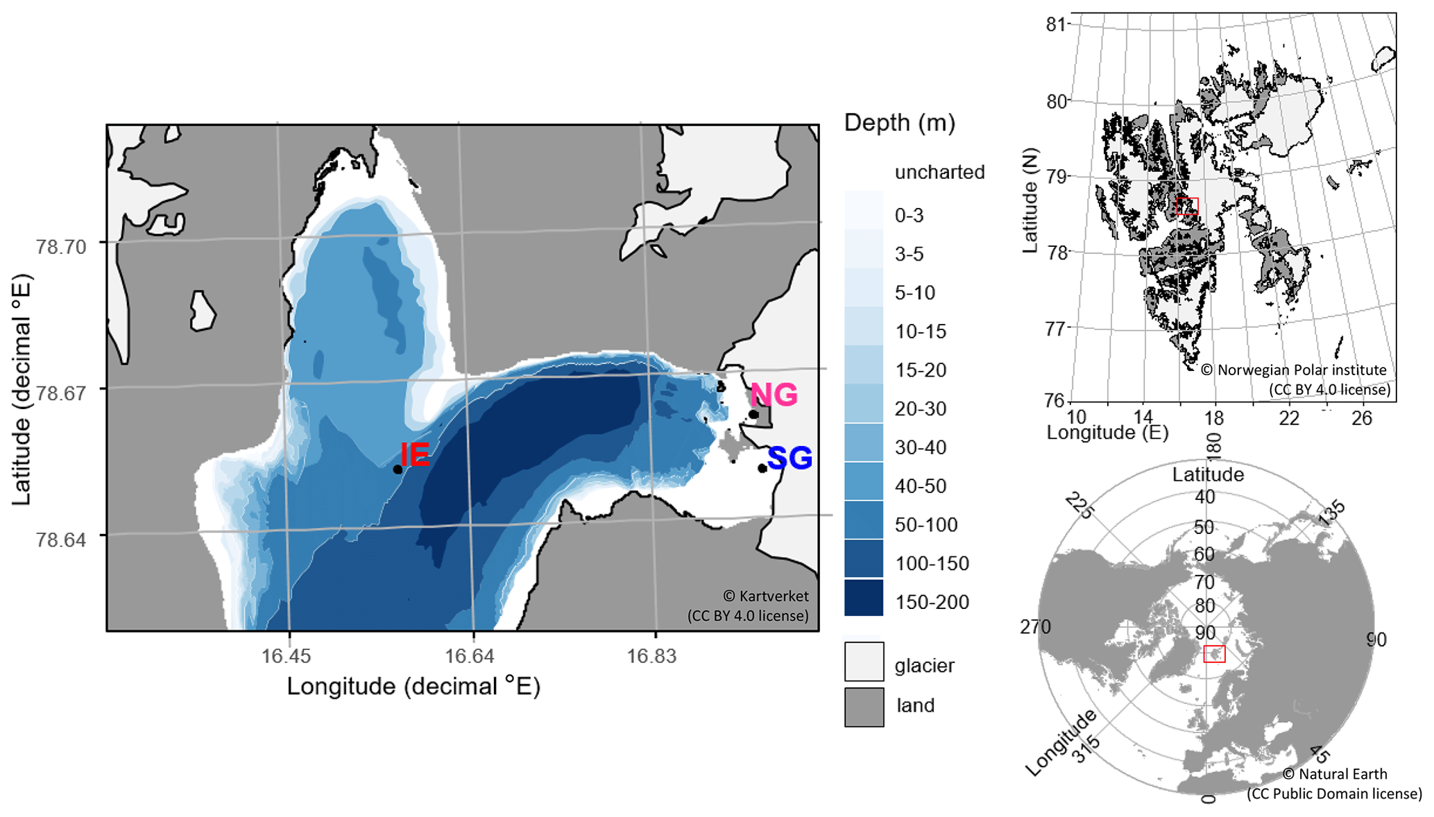
Figure 1 Sampling sites in Billefjorden: (a) detailed Billefjorden map showing the stations at the ice edge (IE), north glacier (NG), and south glacier (SG) on the underlying bathymetric map. White areas are uncharted with water depths of about 30 m at NG and SG. The insets to the right show the location of (b) Billefjorden on a Svalbard map and (c) Svalbard on a pan-Arctic map, marked with red boxes. Land is shown as dark grey, ocean as white, and glaciers as light grey.

Samples were taken at three stations: (1) at the fast-ice edge (IE) – a full marine reference station ($\mathrm{78}{}^{\circ }{\mathrm{39}}^{\prime }{\mathrm{09}}^{\prime \prime }$ N, $\mathrm{16}{}^{\circ }{\mathrm{34}}^{\prime }{\mathrm{01}}^{\prime \prime }$ E), (2) at the southern site of the ocean-terminated glacier terminus (SG) (approx. 20 m water depth) with freshwater outflow observed during the sampling period ($\mathrm{78}{}^{\circ }{\mathrm{39}}^{\prime }{\mathrm{03}}^{\prime \prime }$ N, $\mathrm{16}{}^{\circ }{\mathrm{56}}^{\prime }{\mathrm{44}}^{\prime \prime }$ E), and (3) at the northern site of the glacier terminus (NG) with no clear freshwater outflow observed and a mostly land-terminating glacier front ($\mathrm{78}{}^{\circ }{\mathrm{39}}^{\prime }{\mathrm{40}}^{\prime \prime }$ N, $\mathrm{16}{}^{\circ }{\mathrm{56}}^{\prime }{\mathrm{19}}^{\prime \prime }$ E).

Snow depth and sea ice thickness around the sampling area were measured with a ruler. Sea ice and glacier ice samples were taken with a Mark II ice corer with an inner diameter of 9 cm (Kovacs Enterprise, Roseburg, OR, USA). The temperature of each ice core was measured immediately by inserting a temperature probe (TD20, VWR, Radnor, PA, USA) into 3 mm thick pre-drilled holes. For further measurements the ice cores were sectioned into the following sections: 0–3 and 3–10 cm and thereafter 20 cm long pieces from the bottom to the top. They were packed in sterile bags (Whirl-Pak®, Madison, WI, USA) and left to melt at about 4–15 ^∘C for about 24–48 h in the dark. Sections for chlorophyll a (Chl) measurements, DNA extractions, and algae and bacteria counts were melted in 50 % vol $/$ vol sterile filtered (0.2 µm Sterivex filter, Sigma-Aldrich, St Louis, MO, USA) seawater to avoid osmotic shock of cells (Garrison and Buck, 1986), while no seawater was added to the sections for salinity and nutrient measurements. Salinity was measured immediately after melting using a conductivity sensor (YSI Pro30, YSI, USA). Brine salinity and brine volume fractions were calculated after Cox and Weeks (1983) for sea ice temperatures below −2 ^∘C and after Leppäranta and Manninen (1988) for sea ice temperatures above −2 ^∘C.

Samples of under-ice water were taken using a pooter (Southwood and Henderson, 2000) connected to a handheld vacuum pump (PFL050010, Scientific & Chemical Supplies Ltd., UK). Deeper water at 1, 15, 25 m depths and bottom water at the IE station were taken with a water sampler (Ruttner sampler, 2 L capacity, Hydro-Bios, Germany). Glacial outflow water was sampled in April 2018 close to the SG station using sterile Whirl-Pak® bags. No outflow water was found around the NG station. Cryoconite hole water (avoiding any sediment) was sampled in July 2018 with a pooter on sites known to differ in their biogeochemical settings (Nordenskiöldbreen main cryoconite site (NC) and Nordenskiöldbreen near Retrettøya site (NR) characterized by Vonnahme et al., 2016). Glacier surface ice samples of 1 m length were taken with the Mark II ice corer at the southern side of the glacier on the NC site.

CTD profiles were taken at each station by a CastAway™ (SonTek, Xylem, San Diego, CA, USA). At the SG station an additional CTD profile was taken with a SAIV CTD SD208 (SAIV, Lakselv, Norway) including turbidity and fluorescence sensors. Unfortunately, readings at the other stations failed due to sensor freezing at low air temperatures. Surface light data were obtained from the photosynthetic active radiation (PAR) sensor of the ASW 1 weather station in Petuniabukta (23 m a.s.l), operated by the University of South Bohemia (Láska et al., 2012; Ambrožová and Láska, 2017).

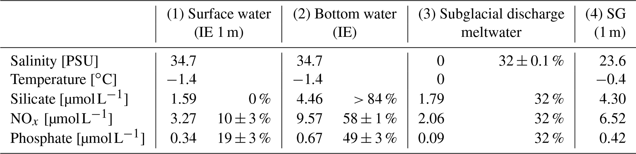
During the sampling days, Billefjorden was overcast. The light regime under the ice was calculated after Masicotte et al. (2018) with a snow albedo of 0.78, a snow attenuation coefficient of 15 m⁻¹ (Mundy et al., 2005), and ice attenuation coefficients of 5.6 m⁻¹ for the upper 15 cm and 0.6 m⁻¹ below (Perovich et al., 1998). For sea ice algae, an absorption coefficient of 0.0025 m² per milligram of Chl was used. The fraction of fjord water versus subglacial meltwater for the water samples was calculated assuming linear mixing (Eqs. A1–A2) of the two salinities (glacial meltwater salinity is 0 PSU; average seawater salinity at IE is 34.7 ± 0.03 standard deviation), since no other water masses in regard to temperature or salinity signature were present (Table 1). The variability in the IE seawater salinity leads to a small (< 1 %) uncertainty in the estimated value of the relative contributions of seawater vs. subglacial meltwater.

Table 1 Properties of (1) marine surface and (2) marine deep water (both station IE), (3) subglacial discharge meltwater, and (4) station SG surface water and the relative contribution of the water types 1 to 3 to form water type 4. The calculations are given in the Supplement and are based on different salinities and nutrients in the four water masses.

2.2 Chemical properties

Nutrient samples of water and melted sea ice and glacier ice were sterile filtered as described above, stored in 50 mL falcon tubes (which were acid washed in 5 % vol$/$vol HCl and Milli-Q® purified water (MQ) rinsed), and kept at −20 ^∘C until processing. Total alkalinity (TA), dissolved inorganic carbon (DIC), and pH samples were sampled in 500 mL borosilicate glass bottles avoiding air contamination, fixed within 24 h with 2 % (final concentration) HgCl₂, and stored at 4 ^∘C until processing.

Nutrients were measured in triplicates using standard colorimetric methods with a nutrient autoanalyzer (QuAAtro39, SEAL Analytical, Germany) using the following instrument protocols: Q-068-05 Rev. 12 for nitrate and nitrite (detection limit is 0.02 µmol L⁻¹), Q-066-05 Rev. 5 for silicate (detection limit is 0.07 µmol L⁻¹), and Q-064-05 Rev. 8 for phosphate (detection limit is 0.01 µmol L⁻¹). The data were analyzed using the software AACE v5.48.3 (SEAL Analytical, Germany). Reference seawater (Ocean Scientific International Ltd., United Kingdom) was used as blanks for calibrating the nutrient analyzer. The maximum differences between the measured triplicates were 0.1 µmol L⁻¹ for silicate and nitrate and 0.05 µmol L⁻¹ for nitrite and phosphate. Concentrations of nitrate and nitrite (NO_x) were used to estimate the fraction of bottom water reaching the surface at SG assuming linear mixing of subglacial meltwater, bottom water (at station IE), and surface water concentration using the NO_x concentration measured at IE and the subglacial meltwater (Table 1). The calculations for these mixing estimates are given in the Appendix (Eqs. A3–A6).

DIC and TA were analyzed within 6 months of sampling as described by Jones et al. (2019) and Dickson et al. (2007). DIC was measured on a Versatile INstrument for the Determination of Total inorganic carbon and titration Alkalinity (VINDTA 3C, Marianda, Germany), following acidification, gas extraction, coulometric titration, and photometry. TA was measured with potentiometric titrations in a closed cell on a Versatile INstrument for the Determination of Titration Alkalinity (VINDTA 3S, Marianda, Germany). Precision and accuracy was ensured via measurements of certified reference materials (CRMs, obtained from Andrew Dickson, Scripps Institution of Oceanography, USA). Triplicate analyses on CRM samples showed mean standard deviations below ±1 µmol kg⁻¹ for DIC and TA.

2.3 Biomass and communities

For determination of algal pigment concentrations, about 500 mL of seawater or melted sea ice was filtered onto GF/F filter (Whatman plc, Maidstone, UK) in triplicates using a vacuum pump (max 200 mbar vacuum) before storing the filter in the dark at −20 ^∘C. Water and melted sea ice for DNA samples were filtered onto Sterivex filters (0.2 µm pore size) using a peristaltic pump and stored at −20 ^∘C until extraction. Algae were sampled in two ways: (1) a phytoplankton net (10 µm mesh size) was pulled up from 25 m, and the samples were fixed in 2 % (final concentration) neutral Lugol and stored at 4 ^∘C in brown borosilicate glass bottles before processing, and (2) water or melted sea ice was fixed and stored directly as described above. For later bacteria abundance estimation, 25 mL of water was fixed with 2 % (final concentration) formaldehyde for 24–48 h at 4 ^∘C before filtering onto 0.2 µm polycarbonate filters (Isopore™, Merck, USA) and washing with filtered seawater and 100 % ethanol before freezing at −20 ^∘C.

Algal pigments (Chl a, pheophytin) were extracted in 5 mL 96 % ethanol at 4 ^∘C for 24 h in the dark. The extracts were measured on a Turner Trilogy 10AU fluorometer (Turner Designs, 2019) before and after acidification with a drop of 5 % HCl. Ethanol of 96 % was used as a blank, and the fluorometer was calibrated using a chlorophyll standard (Sigma S6144). For estimations of algae-derived carbon, a conversion factor of 30 g C per gram of Chl was applied (Cloern et al., 1995). The maximum differences (max − min) between the measured triplicates were under 0.05 µg Chl L⁻¹ unless stated otherwise.

DNA was isolated from the Sterivex filter cut out of the cartridge using sterile pliers and scalpels, using the DNeasy® PowerSoil® Kit following the kit instructions with a few modifications. Solution C1 was replaced with 600 µL of phenol : chloroform : isoamyl alcohol $\mathrm{25}:\mathrm{24}:\mathrm{1}$, and washing with C2 and C3 was replaced with two washing steps using 850 µL of chloroform. Before the last centrifugation step, the column was incubated at 55 ^∘C for 5 min to increase the yield. For microbial community composition analysis, we amplified the V4 region of a ca. 292 bp fragment of the 16S rRNA gene using the primers (515F, GTGCCAGCMGCCGCGGTAA, and 806R, GGACTACHVGGGTWTCTAAT, assessed by Parada et al., 2016). For eukaryotic community composition analyses, we amplified the V7 region of ca. 100–110 bp fragments of the 18S rRNA gene using the primers (forward 5^′-TTTGTCTGSTTAATTSCG-3^′ and reverse 5^′-GCAATAACAGGTCTGTG-3^′, assessed by Guardiola et al., 2015). The Illumina MiSeq paired-end library was prepared after Wangensteen et al. (2018).

For qualitative counting of algal communities, the phytoplankton net and bottom-sea-ice samples were counted under an inverted microscope (Zeiss Primovert, Carl Zeiss AG, Germany) with 10×40 magnification. For quantitative counts, 10–50 mL of the fixed water samples was settled in an Utermöhl chamber (Utermöhl, 1958) and counted. Algae were identified using identification literature by Tomas (1997) and Throndsen et al. (2007). For bacteria abundance estimates, bacteria on polycarbonate filter samples were stained with DAPI (4^′,6-diamidino-2-phenylindole) as described by Porter and Feig (1980), incubating the filter in 30 µL of DAPI (1 µg mL⁻¹) for 5 min in the dark before washing with MQ and ethanol and embedding in Citifluor : Vectashield (4:1) onto a microscopic slide. The stained bacteria were counted using an epifluorescence microscope (Leica DM LB2, Leica Microsystems, Germany) under UV light at 10×100 magnification. At least 10 grids or 200 cells were counted. The community structure of the phytoplankton net haul was used for estimating the contribution of sea ice algae to the settling community based on typical Arctic phytoplankton (von Quillfeldt, 2000) and sea ice algal species (von Quillfeldt et al., 2003) described in the literature.

2.4 In situ measurements and incubations

Vertical algal pigment fluxes were measured using custom-made (Faculty of Science, Charles University, Prague, Czech Republic) short-term sediment traps (6.2 cm inner diameter, 44.5 cm height) at 1, 15, and 25 m under the sea ice anchored to the ice at SG and IE, as described by Wiedmann et al. (2016). Sediment traps were left for 24 h at the SG station and 37 h at the IE station. After recovery, samples for algal pigments were taken, fixed and analyzed as described above. Vertical export fluxes were calculated as described in Eq. (A7). Primary production (PP) was measured based on ¹⁴C-DIC incorporation. Samples were incubated in situ in 100 mL polyethylene bottles attached to the rig of the sediment trap giving identical incubation times. Seawater or bottom sea ice melted in filtered seawater (ca. 20 ^∘C initial temperature to ensure fast ice melt) on-site were incubated with ¹⁴C sodium bicarbonate at a final concentration of 1 µCi mL⁻¹ (PerkinElmer Inc., Waltham, USA). PP samples were incubated in triplicates for each treatment with two dark controls for the same times as the sediment traps. Samples were filtered onto precombusted Whatman GF/F filters (max 200 mbar vacuum) and acidified with a drop of 37 % of fuming HCl for 24 h for removing remaining inorganic carbon. The samples were measured in the Ultima Gold™ scintillation cocktail on a liquid scintillation counter (PerkinElmer Inc., Waltham, USA, Tri-Carb 2900TR), and PP was calculated after Parsons et al. (1984). Dark carbon fixation (DCF) rates were used to estimate bacterial biomass production using a conversion factor of 190 mol POC per mole of CO₂ fixed (Molari et al., 2013).

For testing the effect of the water chemistry on phytoplankton growth, we designed a reciprocal transplant experiment where the phytoplankton communities at SG and IE (1 and 15 m) were transplanted into the sterile filtered water of both SG and IE. Of the water containing the phytoplankton communities of SG or IE, 50 mL was transferred into 50 mL sterile filtered (0.2 µm) seawater of SG or IE in 100 mL polyethylene bottles. The bottles with IE communities were then incubated under the ice at the IE station and those with the SG communities under the ice at the SG station. The aim of the experiment is to test if water chemistry alone is sufficient to increase primary production or if the different communities, light regimes, or temperatures are more important. These samples were incubated and processed together with the other PP incubations at the respective depths as described above.

2.5 Statistics and bioinformatics

Silicate, phosphate, and NO_x concentrations were plotted against salinities and tested for correlations via linear regression analysis using the lm function in R (R Core Team, Vienna, Austria). P values were corrected for multiple testing using the false-discovery rate. Since the primary production estimates of the reciprocal transplant experiments were not normally distributed, came from a nested design, and had heterogeneous variance, a robust nested analysis of variance (ANOVA) was performed to test for significant treatment effects of incubation water with water depth as a nested variable.

The 16S sequences were analyzed using a pipeline modified after Atienza et al. (2020) based on OBITools v1.01.22 (Boyer et al., 2016). The raw reads were demultiplexed, trimmed to a median Phred quality score minimum of 40 and sequence lengths of between 215 and 299 bp (16S rRNA) or between 90 and 150 bp (18S rRNA), and merged. Chimeras were removed using UCHIME with a minimum score of 0.9. The remaining merged sequences were clustered using Swarm (Mahé et al., 2014). The 16S swarms were classified using the RDP Classifier (Wang et al., 2007), and 18S swarms were classified using the SILVA Incremental Aligner (SINA) (Pruesse et al., 2012) with the SILVA SSU 138.1 database (Quast et al., 2012). Further multivariate analyses were performed in R using the vegan package. The non-metric multidimensional scaling (NMDS) plots are based on Bray–Curtis dissimilarities of square-root-transformed and Wisconsin double-standardized operational taxonomic unit (OTU) tables and were used to visualize differences between groups (brackish water at SG − fjord water, sea ice − seawater). Analysis of similarities (ANOSIM) was carried out to test for differences in the communities between the groups (999 permutations, Bray–Curtis dissimilarities).

3 Results

3.1 Physical parameters

The physical conditions of sea ice (temperature T and bulk salinity S; Fig. 2a, b) and surface water (uppermost 4 m under the sea ice, T and S; Fig. 2c, d) at the freshwater-inflow-impacted site SG differed substantially from those at NG and IE. The sea ice and the upper 4 m under the sea ice had consistently lower salinities (< 8 PSU) and higher temperatures (−0.4 to −0.2 ^∘C) at SG compared to NG and IE and also compared to the deeper water masses at SG (salinity > 34.6 PSU; temperature $<-\mathrm{1}$.4 ^∘C) (Fig. 2c, d). Sea ice melt was unlikely because the measured water temperatures and sea ice temperatures were below the freezing point considering the sea ice bulk salinity. The water column at SG was highly stratified with a low-salinity 4 m thick layer under the sea ice, separated by a sharp ca. 1 m thick pycnocline (Fig. 2c, d). In contrast, the water column at IE was fully mixed and at NG only a minor salinity drop from 34.6 to 33.6 PSU occurred within the upper 50 cm under the sea ice (Fig. 2c, d). Sea ice temperature and salinity showed similar variations between the three sites with SG ice having lower salinities and higher temperatures relative to sea ice at the other stations (Fig. 2a, b). At SG, bulk salinities were mostly below 0.7 PSU and calculated brine salinities below 14 PSU, except for the uppermost 20 cm where bulk salinities reached around 1.7 PSU and brine salinity reached 32 PSU (Fig. 2). This resulted in very low brine volume fractions below 5 %, except for the lowermost 10 cm with brine volume fractions up to 9 % (Supplement Table S1). At IE and NG, bulk salinities were mostly above 5 PSU (> 40 PSU brine salinity) and temperatures were below −0.4 ^∘C, which led to brine volume fractions above 6 % in all samples and above 10 % in the bottom 30 cm.

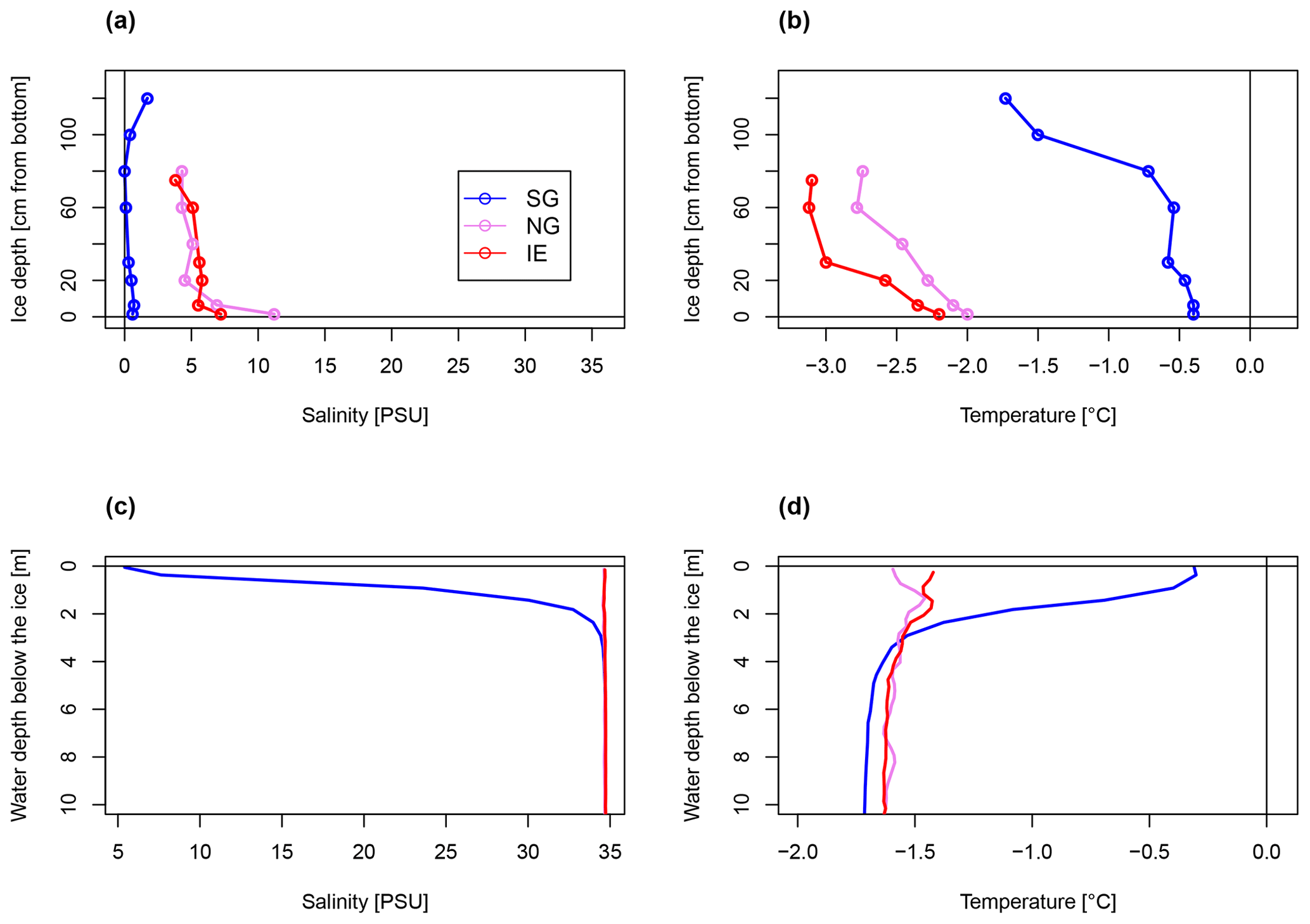
Figure 2 Bulk salinity and temperature profiles in (a, b) sea ice cores (0 cm at the bottom) and (c, d) the water column down to 10 m below the sea ice, of the three stations.

The homogenous temperature and salinity water column profiles at IE and NG stations indicate the presence of only one water mass (local Arctic water; Skogseth et al., 2020). The only additional water mass was subglacial meltwater (salinity of 0 PSU) mixed into the surface layer of SG. Applying a simple mixing model based on the two salinities (34.7 PSU for IE, 0 PSU for glacier) provided an estimation of the fraction of glacially derived water in the surface layer of ca. 85 % in the uppermost 2 m under the sea ice, before decreasing to 0 % at 4 m under the sea ice below the strong halocline. The water sample taken 1 m under the sea ice had a fraction of 32 % glacial meltwater (Table 1). For NG, glacial-derived water contributed only 3 % in the first 50 cm under the sea ice.

The SG station was 33 m deep and about 180 m away from the glacier front. The sea ice was 1.33 m thick and covered by 3 cm of snow. The ice appeared clear with some minor sediment and air bubble inclusions and lacked a skeletal bottom layer. In the water column, a higher potential sediment load was observed as a turbidity peak at the halocline (Fig. 3). Direct evidence of subglacial outflow had been observed at the southern site of the glacier in the form of icing and liquid water flowing onto the sea ice in April 2018, April 2019, and October 2019 (Fig. S4), but this form of subglacial outflow froze before reaching the fjord, which was additionally blocked by impermeable sea ice. The sea ice temperature was between −0.4 ^∘C at the bottom and −1.7 ^∘C at the top (Fig. 2b).

Figure 3 Turbidity profile of the SG station converted to suspended particles.

NG was 27 m deep and about 360 m away from the glacier front. The sea ice was thinner (0.92 m) and the snow cover thicker (6 cm) compared to SG. The ice had a well-developed skeletal layer at the bottom with brown coloration due to algal biomass. The ice temperature ranged between −2 ^∘C at the bottom to −2.7 ^∘C at the top (Fig. 2b). The IE station was about 75 m deep and 50 m away from the ice edge. The sea ice was the thinnest (0.79 m) and the snow cover the thickest (10 cm). Sea ice temperatures were the coldest ranging from −2.2 ^∘C at the bottom to −3.1 ^∘C on the top (Fig. 2b). Loosely floating ice algae aggregates were present in the water directly under the ice. The recorded surface PAR irradiances were similar during the primary production incubation times at SG and IE (for SG, average is 305 µE m⁻² s⁻¹, min is 13 µE m⁻² s⁻¹, and max is 789 µE m⁻² s⁻¹; for IE, average is 341 µE m⁻² s⁻¹, min is 37 µE m⁻² s⁻¹, and max is 909 µE m⁻² s⁻¹). Using published attenuation coefficients, irradiance directly under the ice was 5 µE m⁻² s⁻¹ at IE and with 9 µE m⁻² s⁻¹ higher at SG due to the thinner snow cover.

3.2 Nutrient variability in sea ice and water

Subglacial outflow water and glacial ice had relatively low nutrient levels (in glacial ice, Si(OH)₄ < 0.3 µmol L⁻¹, NO_x < 0.9 µmol L⁻¹, and PO₄ < 0.75 µmol L⁻¹; in outflow, Si(OH)₄ < 1.5–2.0 µmol L⁻¹, NO_x 1.8–2.3 µmol L⁻¹, and PO₄ < 0.1 µmol L⁻¹), but the nutrient concentrations in subglacial outflow water were higher than in most sea ice samples and the depleted surface water (1 m under the sea ice) at the IE. Nutrient concentrations in the fjord were highest in the bottom water (4.0–4.5 µmol L⁻¹ of Si(OH)₄, 9.1–9.6 µmol L⁻¹ of NO_x, 0.7–0.8 µmol L⁻¹ of PO₄) and depleted at the surface and in the sea ice with the exception of the under-ice water (UIW, 0–1 cm under the sea ice) of SG, where NO_x (10 µmol L⁻¹) and silicate (19 µmol L⁻¹) levels were exceptionally high (Fig. 4). We cannot exclude anomalies or sampling artifacts from being responsible for the high UIW values, and therefore we used the values measured 1 m under the sea ice for further calculations in this paper as the surface water reference. SG had overall higher levels of silicate and NO_x compared to the IE at both 1 m below the sea ice (factors of 3 for Si(OH)₄ and 2 for NO_x) and bottom ice (factor of 18 for Si(OH)₄ and 3 for NO_x compared to IE bottom ice) (Fig. 4). Silicate concentrations deeper in the water column were similar at all the stations with values of ca. 4 µmol L⁻¹. Close to the surface silicate was reduced to 1.6 µmol L⁻¹ at 1 m at the IE, while it stayed at 4.3 µmol L⁻¹ at SG (Fig. 4a). In the water column, NO_x and phosphate gradients were similar between the sites. However in sea ice, NO_x concentrations were more than 2 times higher at SG than at the IE. In the bottom 30 cm of sea ice all nutrients had higher concentrations at SG, except for phosphate, which was depleted in the bottom 3 cm of SG but not in the bottom of IE sea ice. In the ice interior at a 50–70 cm distance from the ice bottom, the other nutrients were also depleted at SG, before rising slightly towards the surface of the ice. N:P ratios were generally highest at SG with values above 40, exceeding Redfield ratios in the surface water and sea ice. N:P ratios at the IE were below Redfield ratios in the entire water column and bottom sea ice with values ranging from 10 to 13. A slight increase in NO_x was observed at the sea ice–atmosphere interface at NG and SG.

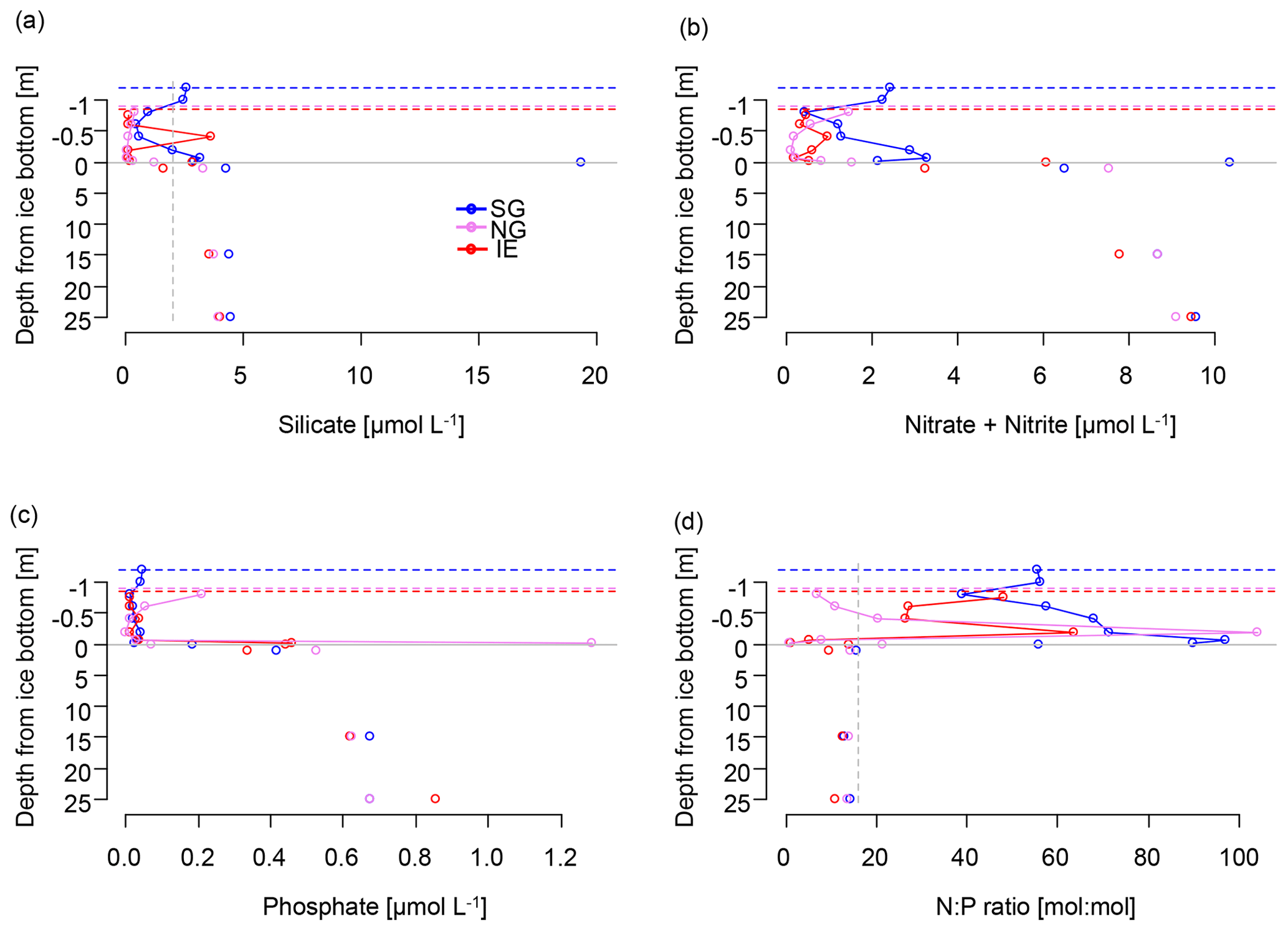
Figure 4 Nutrients in the water column (below grey line) and in sea ice (above the grey line) of (a) silicate with a suggested threshold for limitation marked as dashed grey line, (b) NO_x as nitrate and nitrite, (c) phosphate, and (d) molar N:P ratios with the Redfield threshold of N:P 16:1 marked as dashed grey line indicating potential N limitation. Dashed lines indicate the position of the ice surface, while solid lines show the measured data.

Nutrient versus salinity profiles can give indications of the endmembers (sources) of the nutrients (Fig. 5) with a linear correlation being indicative of conservative mixing. A positive correlation indicates higher concentrations of the nutrients of the saline Atlantic water endmember, while a negative correlation points to a higher concentration in the fresh glacial meltwater endmember. Biological uptake and remineralization could weaken or eliminate the correlation, indicating non-conservative mixing. In the water column at NG and IE, silicate (R²=0.66; p=0.008), NO_x (R²=0.62; p=0.01), and phosphate (R²=0.69; p=0.005) showed conservative positive mixing patterns with higher contributions of Atlantic water (Fig. 5a–c). SG showed a negative correlation for silicate pointing to a higher contribution of glacial meltwater (R²=0.86; p<0.0001). The absence of correlations for NO_x and PO₄ indicates non-conservative mixing pointing towards the relevance of biological uptake and release (Fig. 5d–f). At SG, silicate concentrations were higher with lower salinities. The same pattern was observed in sea ice, with higher silicate and NO_x concentrations in the fresher SG ice, compared to NG and IE (Fig. 5g–i). However, the R² values were lower in particular for Si(OH)₄ (for NO_x, R²=0.18 and p=0.059; for Si(OH)₄, R²=0.41 and p=0.002).

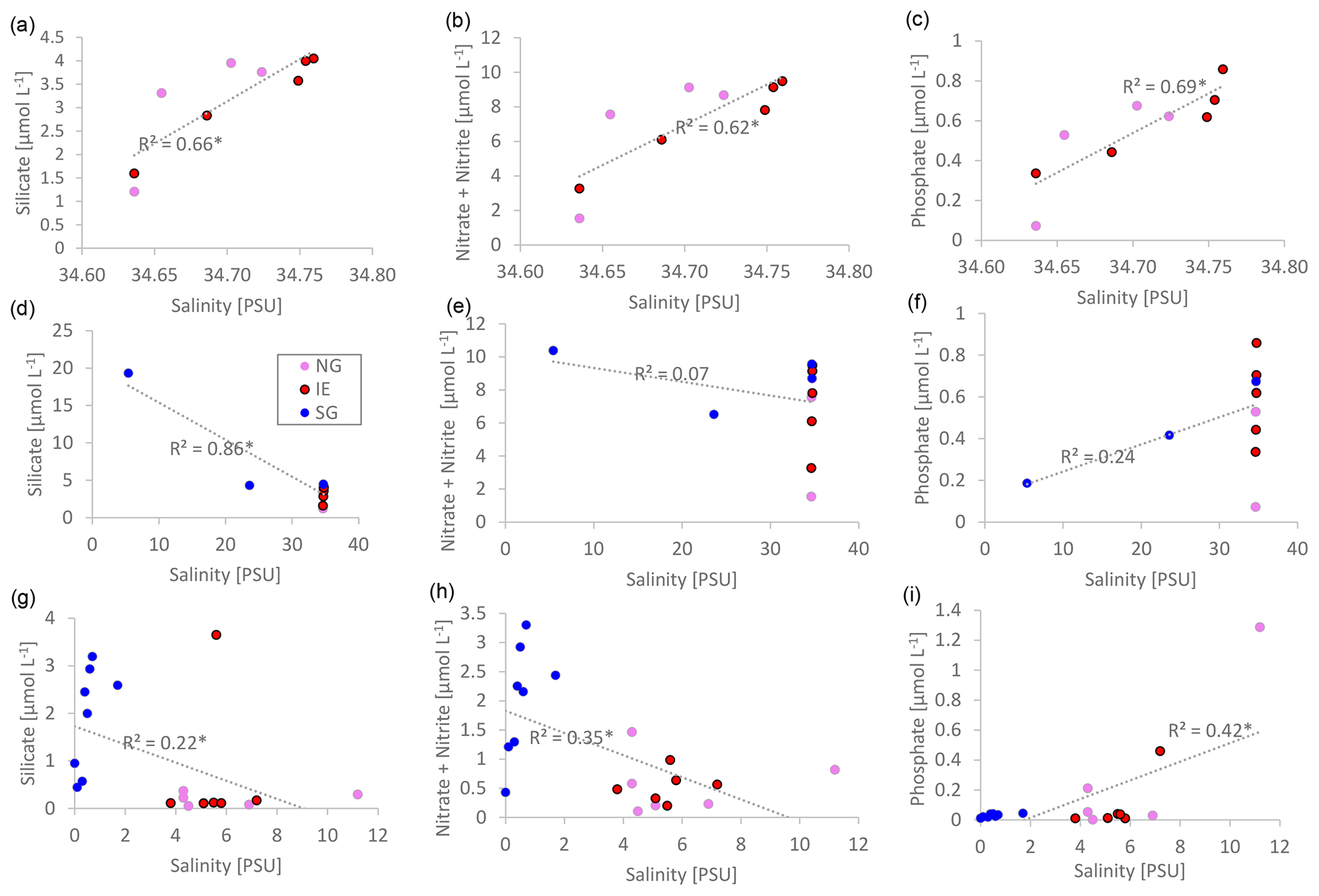
Figure 5 Linear salinity–nutrient correlations of NG and IE water samples (a–c); NG, IE, and SG water stations (d–f); and sea ice samples of NG, IE, and SG (bulk salinities) (g–i). A higher concentration in saline Atlantic water is shown as a positive correlation, and a higher concentration in glacial meltwater is shown as a negative correlation. Significant correlations (p<0.05) are marked with an asterisk beside the R² value.

The contribution of nutrients by upwelling as well as freshwater inflow from glacial meltwater at SG was estimated by linear-mixing calculations for 1 m below the sea ice, avoiding the potential outlier values directly under the ice (Eqs. A1–A6). At 1 m below the sea ice, about 32 ± 0.1 % of the water was derived from glacial meltwater based on salinity-based mixing of glacial meltwater and local Arctic water (Table 1, Eqs. A1–A2). The remaining 68 % came from either bottom-water upwelling (25 m at SG as reference) or surface water (IE values at 1 m under the sea ice as reference). Inorganic nutrients behaved conservatively at the IE reference (Fig. 5a–c), which allows similar mixing calculation of the bottom-water fraction. Based on linear mixing of inorganic nutrients, 58 ± 1 % of NO_x and 49 ± 3 % of PO₄ was provided by subglacial upwelling (Table 1). For silicate, higher concentrations were required in the bottom water of subglacial meltwater at the glacier front to explain the very high surface concentrations measured. Considering the estimated NO_x and PO₄ fractions, the overall fraction of nutrients derived from upwelling was about 53 %. The overall budget 1 m under the sea ice was 32 ± 0.1 % glacial meltwater, 53 ± 3 % subglacial upwelling (marine bottom water), and 15 ± 3 % horizontal transport (surface water).

3.3 Carbon cycle

Net primary productivity (NPP) was overall 1 order of magnitude higher at SG than at IE, with the highest production value occurring within the brackish layer under the ice at SG (5.27 mg m⁻³ d⁻¹; Figs. 6, 7). Within this layer, Chl values were also about 2 times higher compared to IE (21 mg m⁻³ at SG, 9.1 mg m⁻³ at IE), and also the Chl-specific productivity in this layer exceeded values at the other stations (Table 2). Within sea ice, a slightly different pattern emerged. While the primary productivity in the bottom sea ice (0–3 cm) was 2 times higher at SG compared to IE, Chl values were 2 orders of magnitude lower (Fig. 6). This indicates high Chl-specific production at SG (5.6 mg C per milligrams of Chl per day in the sea ice and 11.4 mg C per milligrams of Chl per day integrated over a 25 m depth). At the IE, the contribution of released ice algae to algal biomass in the water column was higher and the overall vertical Chl flux was about 1.5 times higher than at SG at 25 m depth. Bacterial biomass was comparable at both stations with biomass concentrations within the ice higher than in the water column. Bacterial activity (based on DCF) was comparable in the bottom sea ice at the two sites; however, it was 63 times higher in the brackish surface water of SG leading to very high growth rate estimates (Table 2) of 6 mg C m⁻³ d⁻¹. Due to a conversion factor from a very different habitat (Molari et al., 2013), the absolute bacterial growth rate estimates are likely overestimations.

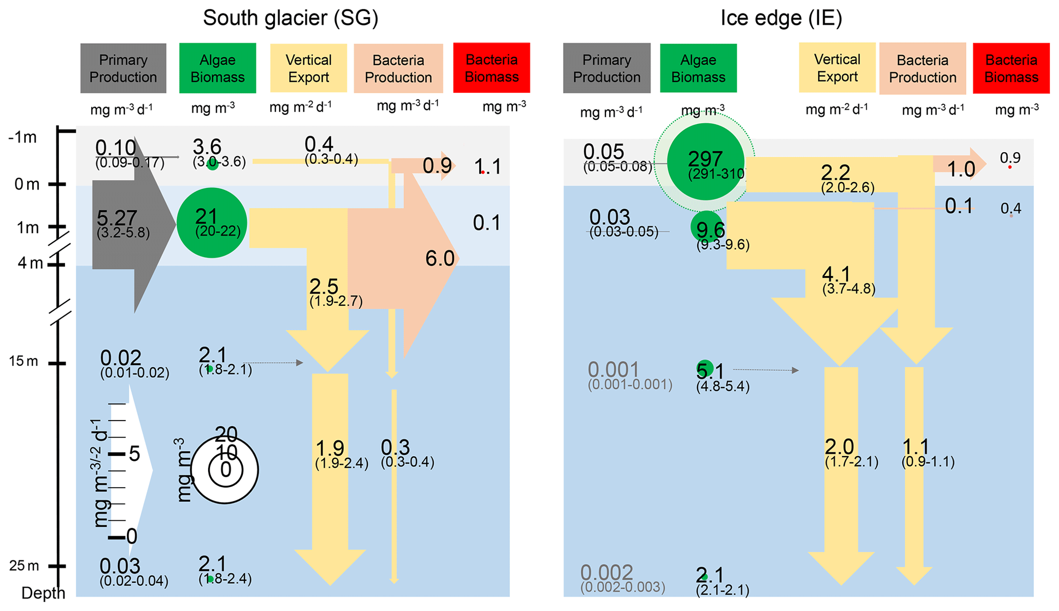
Figure 6 Schematic representation of the C cycle at SG and IE stations. All units are in milligrams of C with the median given in the circles and arrows and the minimum and maximum in brackets below. Depth of 0 m is at the sea ice–water interface. Grey arrows indicate net primary production with its height scaled to the uptake rates. Green circles show standing-stock algae biomass converted from Chl to C (conversion factor is 30 g C per gram of Chl; Cloern et al., 1995) with its diameter scaled to the concentrations, except sea ice at IE with the light green circle scaled 1 order of magnitude higher. Yellow arrows indicate vertical export of chlorophyll converted to C (conversion factor is 30 g C per gram of Chl; Cloern et al., 1995) with the contribution of sea ice algae and phytoplankton estimated by the fraction of typical sea ice algae in phytoplankton net hauls and the width of the arrows scaled to the fluxes. Orange arrows indicate bacterial biomass production based on dark carbon fixation (conversion factor is 129 g C per gram of DIC; Molari et al., 2013) with the arrows scaled to the values. Red circles to the right are bacteria biomass assuming 20 fg C per cell in the bottom sea ice and UIW. The grey area represents sea ice, the light blue area a brackish water layer, and the darker blue area deeper saline water layers.

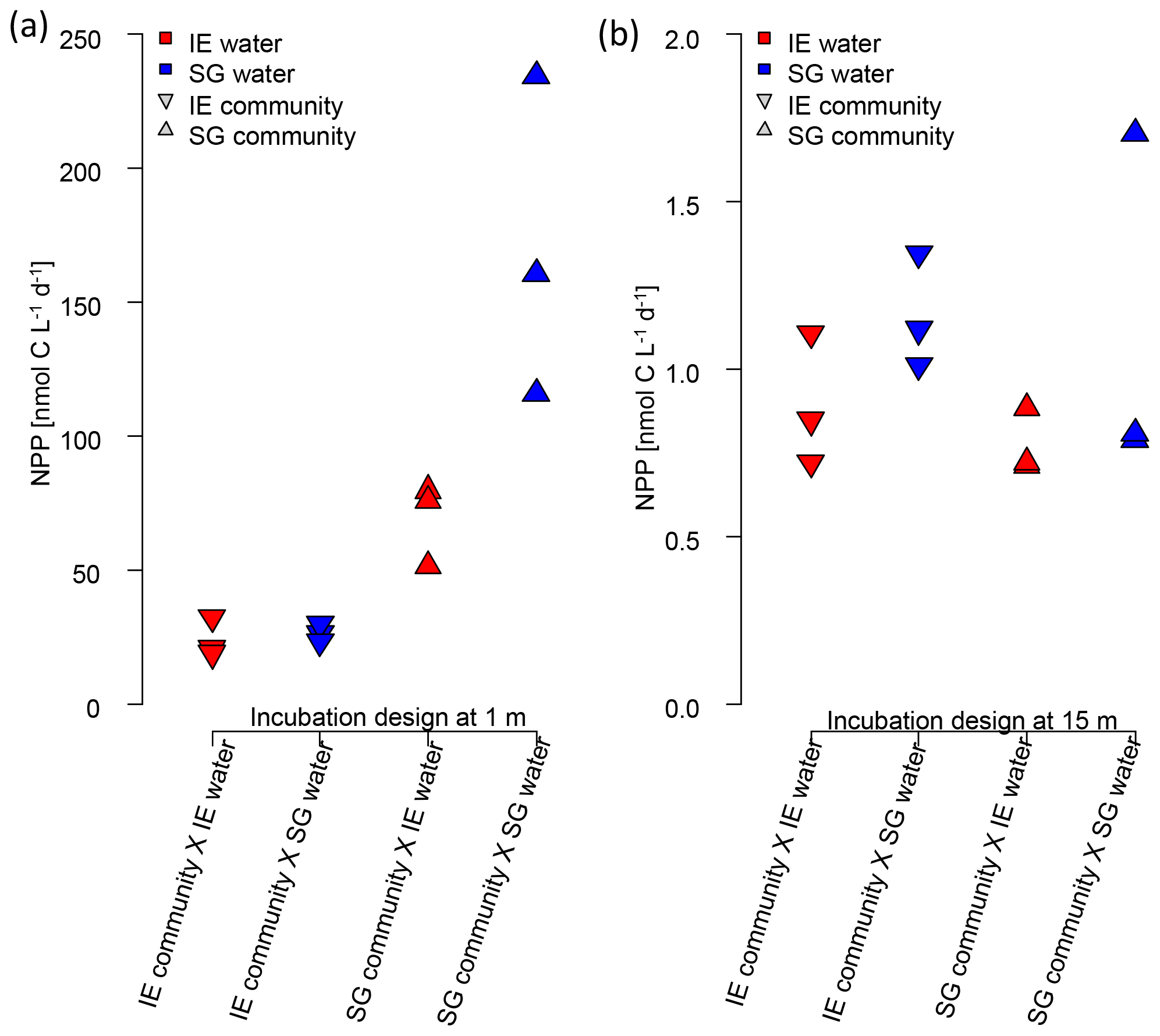
Figure 7 Impact of water source on primary production assessed via a reciprocal transplant experiment. Primary production of IE and SG communities incubated in sterile filtered water originated from either station at (a) 1 m and (b) 15 m depth. The symbols show the source of the community, and the colors indicate the source of the sterile filtered incubation water. The type of incubation water (color) explains the variation in a nested ANOVA with community (symbol) and depth as nested constrained variables and water source (color) as an explanatory variable (p=0.0038; F=10.88).

Table 2 Integrated standing-stock biomass of Chl and fluxes of Chl and C, fractions of the different fluxes and standing stocks, and bacterial production based on dark carbon fixation (DCF).

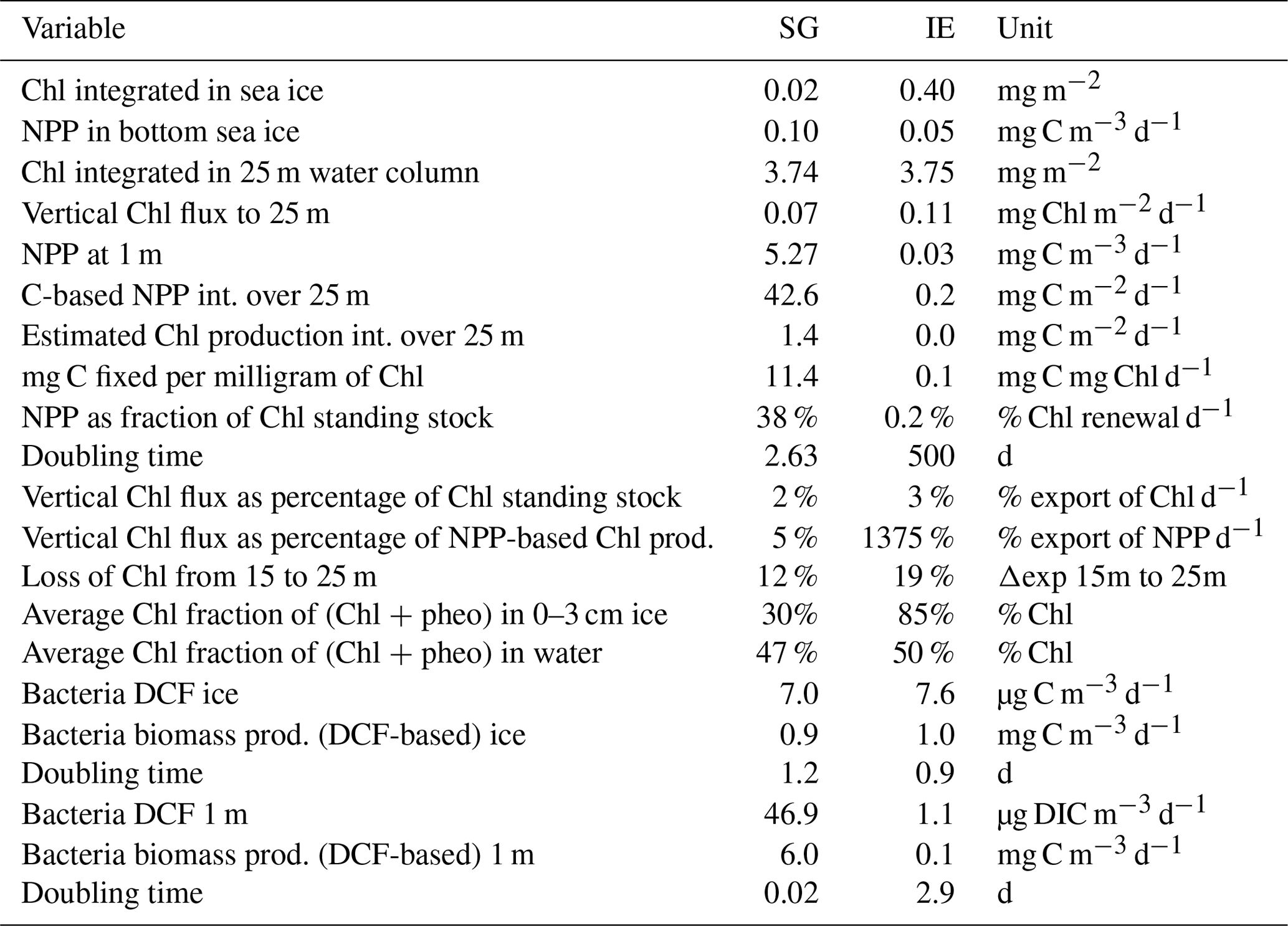
Integrated Chl values over the uppermost 25 m of the water column were nearly identical for SG and IE with values of about 3.75 mg Chl m⁻² (Table 2). The fraction of Chl was highest at IE (85 %) and lowest at SG (30 %) (Table 2). The integrated NPP was considerably higher at SG (42.6 mg C m⁻² d⁻¹ at SG, 0.2 mg C m⁻² d⁻¹ at IE), while the vertical export of Chl was about 3 times higher at IE than at SG. This leads to more (14 times) vertical export based on the sediment trap measurements than production at IE and considerably lower (5 %) export than production at SG (Table 2). Relative to the standing-stock biomass of Chl at IE, 0.2 % of the Chl was renewed daily by NPP at IE and 3 % was vertically exported daily at IE, which would relate – assuming the absence of advection – to a daily loss of 3 % of the standing-stock Chl. At SG, 38 % was renewed per day, while 2 % was exported. As grazing was not estimated in this study, the suggested loss terms of Chl based on the sediment trap data are likely underestimations. This leads to an accumulation of biomass of 38 % d⁻¹ and a doubling time of about 2.6 d. Bacterial-growth doubling times were estimated to be between minutes (SG water) and days (IE water) but within hours in sea ice (Table 2).

Considering the N demand based on the carbon-based PP measurement (16 mol C per mole of N after Redfield, 1934), about 2 µmol N L⁻¹ per month (equivalent to 32 % of 1 m value for NO_x) was needed to sustain the PP measured at SG. Assuming constant PP and steady-state nutrient conditions, 32 % of the surface water had to be replaced by subglacial upwelling per month to supply this N demand via upwelling. Since only 62 % of the upwelling water was entrained bottom water, the actual vertical water replenishment rate would be 52 % per month. Assuming a 2 m freshwater layer under the ice, this translates to flux of about 1.1 m³ m⁻² per month. Considering a distance of 250 m to the glacier front and a width of 1.6 km of the SG bay, this translates to a minimum of about 422 000 m³ per month.

The reciprocal transplant experiment aimed to show the effect of water chemistry on primary production in the absence of effects related to different communities, temperature, or light. The results (Fig. 7) showed clearly that the higher NPP at SG, compared to NG, was related to the nutrient concentrations (nested ANOVA, p=0.0038 and F=10.88). In any combination, sterile filtered water from SG had a fertilizing effect on both SG and IE communities, increasing PP of IE communities by approx. 30 %. SG communities of the most active fresh surface layer (1 m) fixed twice as much CO₂ when incubated in the same water, compared to incubations in the IE water.

3.4 Bacterial, archaeal, and eukaryotic communities

After bioinformatic processing 13 043 bacterial and archaeal (16S rRNA) OTUs, belonging to 1208 genera with between 9708 and 331 809 reads, were retained. Differences between the bacterial 16S sequences of the various sample types indicated that they can be used as potential markers for the origin of the water (Fig. 8). Sea ice and water communities are clearly separated (ANOSIM, p=0.004 and R=0.35) with no overlapping samples (Fig. 8a). Generally IE and NG communities were very similar, while sea ice and under-ice water communities at SG were significantly different (ANOSIM, p=0.001 and R=0.593) from the other fjord samples. The NMDS also showed separation of 16S communities along a gradient from subglacial communities towards fjord communities, with SG communities being in between fjord and subglacial communities (Fig. 8a). Bacterial communities at SG in the bottom layer of the sea ice and the brackish water layer were more similar to subglacial outflow communities than the other samples in both 2018 and 2019. Six OTUs were unique to the glacial outflow and SG surface (closest relatives Fluviimonas, Corynebacterineae, Micrococcinae, Hymenobacter, and Dolosigranuum), which comprise 6.6 % of their OTUs. The community structure of supraglacial ice was very different from any other sample. In the most abundant genera clear differences can also be detected (Fig. S1). Flavobacterium was most abundant in sea ice and UIW samples in both 2018 and 2019 at SG, but it was rare or absent in the other samples. Aliiglaciecola was characteristic of NG sea ice and UIW samples. Paraglaciecola was abundant in NG and IE sea ice and UIW samples, and Colwellia was abundant in all sea ice and UIW samples. In seawater samples the genus Amphritea was more abundant. Pelagibacter was abundant in all samples. Glacial outflow water was dominated by Sphingomonas and glacier ice by Halomonas, which were rare or absent in the other samples.

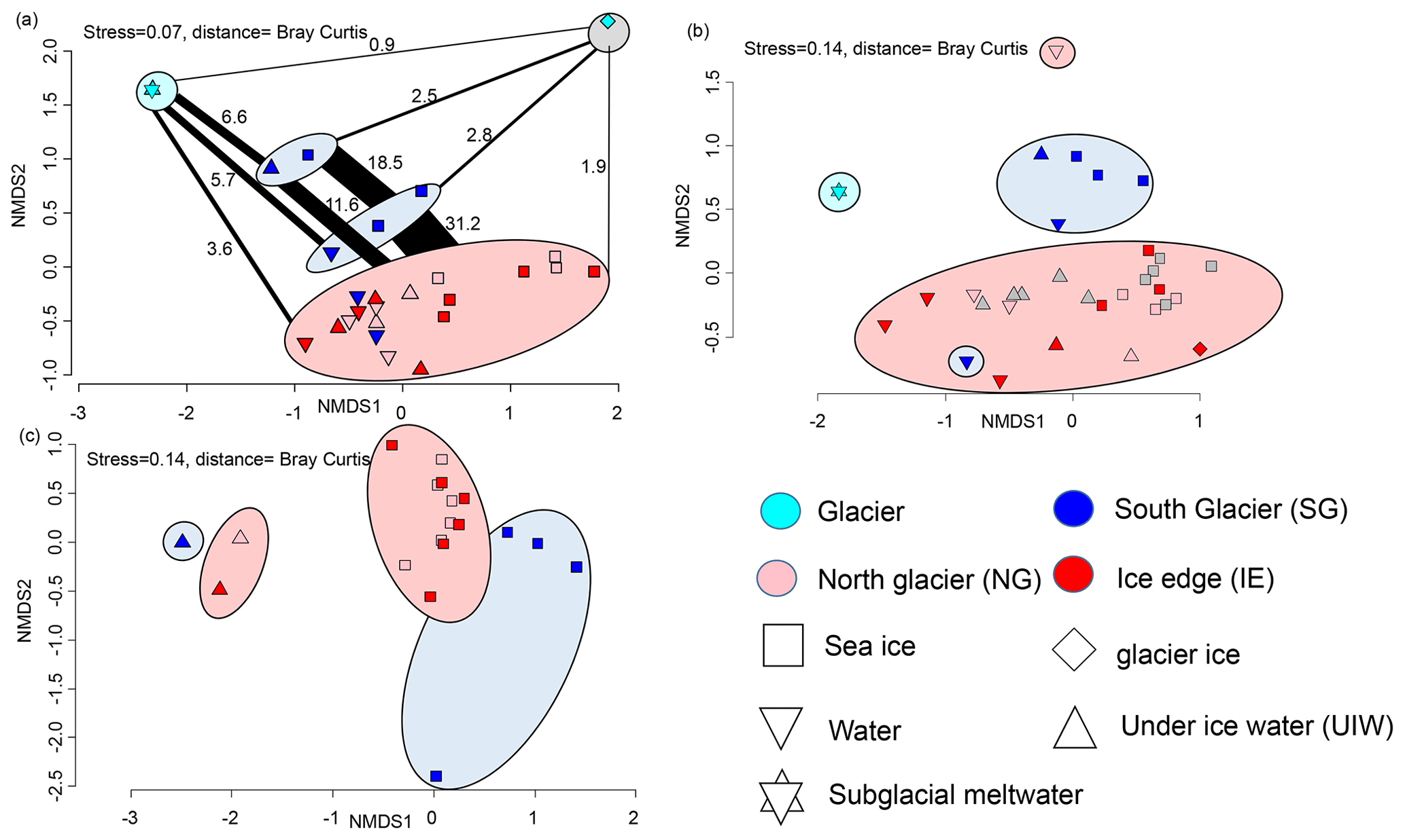
Figure 8 (a) NMDS plot of microbial community structure based on 16S data (stress is 0.07), including samples from April 2018. Groups highlighted in eclipses: glacier ice (top right in grey eclipse), undiluted subglacial outflow (top left in cyan eclipse), surface samples (UIW, sea ice) at station SG 2019 (top blue eclipse), surface samples (1 m water, sea ice) at station SG 2018 (bottom blue eclipse), and others including deeper water samples at SG (bottom in red eclipse). The fraction of shared OTUs (in %) are shown as lines scaled to the fraction (%) of shared OTUs. (b) NMDS plot of community structure based on 18S data (stress is 0.14), including samples from April 2018 with the surface water sample of NG as an outlier on top and a surface water sample of SG as an outlier in the red reference cluster. (c) NMDS plot based on algae abundances in sea ice and UIW based on light microscopic counts (stress is 0.14).

The eukaryotic community (18S rRNA) consisted of 4711 OTUs, belonging to 535 genera, with between 2204 and 15 862 reads. Overall, the same NMDS clustering has been found as for the 16S rRNA sequencing. We found distinctive communities in the sea ice and 1 m layer under the sea ice at SG, being significantly different (ANOSIM, p=0.001 and R=0.456) to the other samples (Fig. 8c). In fact, the SG surface communities were more similar to the outflow community (Fig. 8c). The clear differentiation between all sea ice and water column communities was also visible in the 18S rRNA samples (ANOSIM, p=0.005 and R=0.192). As for the 16S communities, the abundant genera also differed between the groups (Fig. S2). The cryptophytes Hemiselmis and Geminigeraceae were abundant at SG but rare at the other sites. Dinophyceae, Imbricatea (Thaumatomastix), and Bacillariophyceae were abundant in all samples with diatoms being mostly more abundant in sea ice or UIW. The Chytridiomycota division of Lobulomycetaceae was abundant in water samples from 2018 but not 2019. Subglacial outflow water was dominated by unclassified Cercozoa and Bodomorpha.

In total 22 different taxa were detected by microscopy. The community composition was clearly separated between sea ice and water samples. Furthermore sea ice species composition at SG differed from NG and IE (Fig. 8c). SG sea ice was completely dominated by unidentified flagellates (potentially Hemiselmis, Geminigeraceae, and Thaumatomastix based on 18S sequences), with the exception of the 70–90 cm layer with high abundances of Leptocylindrus minimus. Sea ice samples at NG and IE were dominated by the typical ice algae Navicula and Nitzschia frigida. Water samples were more diverse with high abundances of Fragillariopsis, Coscinodiscus, and Chaetoceros. Overall, diatoms dominated most samples at NG and IE in sea ice and water samples.

4 Discussion

The hydrography, sea ice properties, water chemistry, and bacterial communities at SG provide clear evidence for submarine discharge and upwelling at a shallow tidewater outlet glacier under sea ice, a system previously not considered for subglacial upwelling processes. Briefly, our first hypothesis that submarine discharge also persists in early spring, supplying nutrient-rich glacial meltwater and upwelling of bottom fjord water to the surface, has been confirmed as discussed in detail below.

4.1 Indications of subglacial discharge and upwelling

The physical properties at SG were distinctly different to stations NG and IE. In contrast to NG and IE, the marine-terminating SG site had a brackish surface water layer of 4 m thickness under the sea ice and low sea ice bulk salinities below 0.7 PSU, with the exception of the uppermost 20 cm with a bulk salinity of 1.7 PSU. The sea ice bulk salinity is comparable to sea ice in the nearby tidewater-glacier-influenced Tempelfjorden (Fransson et al., 2020) and brackish Baltic sea ice (Granskog et al., 2003). We excluded surface melt or river runoff as freshwater sources for the following reasons. With air temperatures below freezing point during the sampling periods, surface runoff based on snowmelt was not possible and no melting was observed during fieldwork. In addition, there are no major rivers known to flow into the main bay studied (Adolfbukta), due to the small catchment areas (Norwegian Polar Institute, 2020). We did observe some subglacial runoff at the southern site of the glacier (close to SG), but this outflow water froze before it reached the fjord, which was additionally blocked by 1.33 m thick sea ice cover. The sea ice cover would also block any inputs by atmospheric precipitation, considering the impermeable sea ice conditions especially at SG with brine volume fractions below 5 % (Golden et al., 1998; Fransson et al., 2020). If surface runoff were present, we would also expect a similar pattern at the NG site. In fact, due to the closer proximity to the southward-facing mountains and higher sea ice permeability, NG would be more likely influenced by surface runoff than SG would be. Other potential freshwater sources could be related to subaqueous melt of the glacier terminus (Holmes et al., 2019; Sutherland et al., 2009), icebergs (Moon et al., 2018), or ice melange (Mortensen et al., 2020). However, in the absence of Atlantic water inflow, which is blocked by a shallow sill at the entrance of Billefjorden (Skogseth et al., 2020), water temperatures were consistently below the freezing point (max −0.2 ^∘C), and no Atlantic inflow water (temperature ≥ 1 ^∘C and salinity ≥ 34.7 PSU; Skogseth et al., 2020) was detected at any station. These low water temperatures do not allow glacier terminus ice to melt. Besides, Billefjorden is not characterized by large quantities of icebergs or ice melange as described for Greenland glaciers (Moon et al., 2018; Mortensen et al., 2020). However, glacier terminus ice melt is likely more important in systems with Atlantic water inflows, such as Greenland or Svalbard fjords without a shallow sill (e.g., Kongsfjorden and Tunabreen; Holmes et al., 2019). Sea ice may melt at lower temperatures compared to glacial ice, but the absence of typical sea ice algae in the water column at SG and the low salinity of the sea ice indicated that this was not the case. In fact, sea ice with a salinity of 1.5 PSU (measured at SG) would melt at −0.08 ^∘C (Fofonoff and Millard, 1983), but the water and ice temperatures did not exceed −0.2 ^∘C. At this temperature the brackish surface water and meltwater of the submarine discharge would be supercooled. We did find a 1.5 cm layer of frazil ice on the bottom of the SG sea ice showing that this did have some influence on sea ice formation. The subglacial meltwater would need to introduce some heat, allowing the meltwater to reach the surface as liquid water. A temperature maximum at the sea ice–water interface supports this hypothesis. This heat may also lead to basal sea ice melt adding freshwater closer to the glacier front and main plume. However, sea ice melt as a freshwater source cannot explain the low salinity of the sea ice itself. Consistent with our study Fransson et al. (2020) also found a substantial amount of freshwater in the sea ice in Tempelfjorden (approx. 50 % meteoric water fraction) in a year with large glacier meltwater contribution further supporting the presence of subglacial discharge under sea ice in our study. Fransson et al. (2020) suggested the combination of low salinities with high silicate concentrations as an indicator of glacial meltwater contributions, which was also the case in our study. In addition, the overall low sea ice salinity and sediment inclusions at SG cannot be explained by sea ice melt but must originate from another source. Clear evidence for outflow also comes from the visual observations of subglacial outflow exiting the land-terminating part south of the glacier in October 2019, April 2018, and April 2019, which we assume also occurred under the marine-terminating front. In fact, subglacial outflows in spring are a common phenomenon observed at various other Svalbard glaciers with runoff originating from meltwater stored under the glacier from the last melt season and released by changes in hydrostatic pressure or glacier movements (Wadham et al., 2001). Active subglacial drainage systems in winter have also been described elsewhere, and they can be sustained by geothermal heat or frictional dissipation, groundwater inputs, or temperate ice in the upper glacier (Wilson et al., 2013; Schoof et al., 2014). This meltwater has also been found to be rich in silicate due to the long contact with the subglacial bedrock during its storage over winter (Wadham et al., 2001; Fransson et al., 2020). We therefore suggest that early spring subglacial discharge is not unique to Billefjorden but likely occurs at all polythermal or warm-based marine-terminating glaciers.

4.2 Potential magnitude of subglacial discharge and upwelling

Considering the slow tidal currents in our study area (< 22 m per 6 h tidal period; Kowalik et al., 2015) and wind mixing blocked by sea ice, a potential source of the freshwater within Billefjorden may be meltwater introduced during the late-summer-to-fall melt season and remaining throughout winter. Hence, the question of how much subglacial meltwater reaches the surface in what timeframe is important. We estimated that the surface water was most likely exchanged on timescales of days to weeks. Even slow vertical mixing would be capable of eroding the halocline in over 6 months since the last melt season. The turbidity peak that we observed at the halocline would also settle out in a short time (weeks) if not replenished by fresh inputs (Meslard et al., 2018). We determined vertical export flux to account for approximately 4 % of the Chl standing stock at 25 m (Table 2). Considering that glacial sediment settles typically much faster than phytoplankton due its higher density, this suggests that the turbidity peak would erode within days to weeks without fresh sediment inputs via upwelling (Meslard et al., 2018). Furthermore, the inorganic nitrogen demand for the measured primary production would consume the present nutrients in a few (approx. 2) months. Assuming a steady state, the nutrient uptake by phytoplankton primary production would require an upwelling-driven water flux of at least 1.1 m³ m⁻² per month.

Microbial communities (16S rRNA and 18S rRNA) in SG UIW and sea ice were similar to the subglacial outflow water. Bacterial communities (16S rRNA) at SG shared 6.6 % of their OTUs with subglacial outflow communities, which is twice as much as those at NG and IE (3.6 %) shared with the outflow communities. Considering the estimated bacterial production and biomass (Table 2) at SG, the doubling time of the bacteria would be between 0.5 and 7 h (Table 2). However, the use of a conversion factor for biomass production based on sediment bacterial data adds uncertainty to the estimation of the bacterial doubling time. Estimates reported from Kongsfjorden in April are indeed longer (3–10 d; Iversen and Seuthe, 2011), as are other Arctic bacterioplankton doubling-time estimates ranging from 1.2 d (Rich et al., 1997) to 2.8 d (de Kluijver et al., 2013) to weeks (2 weeks in Rich et al., 1997; 1 week in Kirchman et al., 2005).

Based on the growth in the range of hours to days, the distinctive community at SG would have changed to a more marine community on timescales of weeks, assuming only growth of marine OTUs at SG and settling out or grazing of inactive glacial bacteria taxa. Thus, we suggest that the presence of OTUs shared between SG and the glacial outflow may indicate a continuous supply of a fresh inoculum to sustain these taxa.

The amount of discharge and upwelling was estimated using hydrographic data. In our study, three water masses were distinguished: (i) subglacial outflow (SGO) with low salinity (0 PSU), relatively high temperatures (>0 ^∘C), and high silicate concentrations (Cape et al., 2019); (ii) deep local Arctic water (DLAW) entrained from approx. 20 m with low temperatures (−1.7 ^∘C), high salinities (34.7 PSU), and high nutrient concentrations (Skogseth et al., 2020); and (iii) surface local Arctic water (SLAW) with the same temperature and salinity signature as the DLAW but depleted in nutrients (Skogseth et al., 2020). Nutrients were depleted in the UIW but not at 15 m depth, showing that the nutricline was shallower than 15 m. Hence, subglacial discharge at a glacier terminus depth of 20 m would be sufficient to cause upwelling of nutrient-rich DLAW to the surface. In fact, our mixing calculations (Eqs. A1–A6) estimate that 32 % of the SG water 1 m under the sea ice was derived by SGO, which pulled 1.6 times as much (53 % DLAW: 32 % SGO is ratio of 1.6) DLAW with it during upwelling. Fransson et al. (2020) found that 30 %–60 % of glacier-derived meltwater was incorporated into the bottom sea ice at the glacier front of Tempelfjorden, which is comparable to our study, again indicating that early spring subglacial discharge and the resulting formation of sea ice with low porosity is a widespread process at marine-terminating glacier fronts on Svalbard. Uncertainties with these estimates may be related to sea ice melt as an additional freshwater source and to slightly different nutrient concentrations directly in the SG subglacial discharge compared to the sampled subglacial outflow at some distance.

4.3 Importance of subglacial discharge and upwelling under sea ice

To our knowledge, our study currently provides the only available estimate of subglacial upwelling in early spring. Our study suggests that subglacial upwelling in spring results in a small volume transport of only about 1.1 m³ m⁻² per month (approx. 2 m³ s⁻¹) in Billefjorden. This estimate is based on the flux of nutrient-rich bottom water needed to maintain the measured primary production assuming steady-state conditions and is therefore a rough, but conservative, estimate. Due to logistical limitations, we could only sample the subglacial outflow at some distance from and not directly at the SG site. Consequently, submarine discharge at SG may have slightly different nutrient concentrations due to potentially different bedrock chemistry. The most comparable estimate on the magnitude of the upwelling is available at Kronebreen for summer. This Svalbard tidewater glacier is of similar size and had upwelling rates 1 order of magnitude higher compared to our study (31–127 m³ s⁻¹; Halbach et al., 2019). Due to their respective sizes, summer subglacial upwelling flux in Greenland is 2 to 4 times higher than at Kronebreen (250–500 m³ s⁻¹; Carroll et al., 2016). In our study about 1.6 times as much bottom water from about 20 m (DLAW) as subglacial outflow water (SOW) reached the surface at SG (entrainment factor of 1.6 – see above). The entrainment factor is mostly dependent on the depth of the glacier front (Carroll et al., 2016). In fact, the glacier terminus at SG was shallower (approx. 20 m) than any other studied tidewater glacier on Svalbard (70 m depth at Kronebreen; Halbach et al., 2019) or Greenland (> 100 m; Hopwood et al., 2020). Hence, the higher summer entrainment factors estimated in Kongsfjorden (3; Halbach et al., 2019) and Greenland (6 to 30, Hopwood et al., 2020) are not surprising. Glacier terminus depth appears to be the main control of entrainment rates, likely independent of the time of the year. However, turbulent mixing may cause increased entrainment during times of very high subglacial discharge rates. The higher entrainment factors in Greenland also lead to more saline water reaching the surface, and the strongly stratified brackish surface layer observed at SG has not been observed at these deep tidewater glaciers (e.g., Mortensen et al., 2020). Kronebreen is the most comparable tidewater glacier in terms of glacier terminus depth and entrainment rate. Although the estimated entrainment factor was low at Kronebreen (3), subglacial upwelling substantially increased summer primary production in Kongsfjorden (Halbach et al., 2019). In spite of the shallow depth and the low discharge and entrainment rate of our study, subglacial upwelling appears to be the main mechanism to replenish bottom water with high nutrient concentrations to the surface and can substantially increase spring primary production due to (i) subglacial outflow below (approx. 20 m) the nutricline (< 15 m), (ii) the absence of any other terrestrial inputs, (iii) Atlantic water blocked by a shallow sill (Skogseth et al., 2020), (iv) very weak tidal currents (Kowalik et al., 2015), (v) wind mixing blocked by sea ice in Billefjorden, and (vi) undiluted subglacial meltwater having lower nutrient concentrations than the DLAW.

4.4 Importance for under-ice phytoplankton

Our main finding was that (i) higher irradiance, (ii) a stratified surface layer, and (iii) increased nutrient supply via subglacial discharge and upwelling allowed increased phytoplankton primary production at SG. The ice edge station (IE) was light- and nutrient-limited and supported lower phytoplankton primary production.

4.4.1 Increased light

Despite the subglacial discharge and upwelling, the negative effect of light limitation with the massive sediment plumes in summer (Pavlov et al., 2019) was not observed in early spring. We did measure a small turbidity peak under the SG sea ice, but the values were comparable to open fjord systems in summer (Meslard et al., 2018; Pavlov et al., 2019), where light is sufficient for photosynthesis. Under-ice phytoplankton blooms are typically limited by light, which is attenuated and reflected by the snow and sea ice cover (Fortier et al., 2002; Mundy et al., 2009; Ardyna et al., 2020). Some blooms have been observed, mostly under snow-free sea ice, such as after snowmelt (Fortier et al., 2002), under melt ponds (Arrigo et al., 2012, 2014), after rain events (Fortier et al., 2002), or at the ice edge related to wind-induced Ekman upwelling (Mundy et al., 2009). In our study however, light levels available for phytoplankton growth were low compared to in other under-ice phytoplankton bloom studies (Mundy et al., 2009; Arrigo et al., 2012), but they were higher at SG than at IE. This can be explained through the combined effects of sea ice and snow properties at SG. Light attenuation in low-salinity sea ice is typically lower due to a lower brine volume (Arst and Sipelgas, 2004). Also, lower sea ice algae biomass and thinner snow cover due to snow removal with katabatic winds (e.g., Braaten, 1997; Láska et al., 2012) leads to less light attenuation and a lower albedo. Our estimates showed that about twice as much light reached the water at SG compared to at IE, in spite of the thicker sea ice cover. The estimated light levels of 5 and 9 µE m⁻² s⁻¹ were above the minimum irradiance (1 µE m⁻² s⁻¹) required for primary production (Mock and Gradinger, 1999). Hence, the increased light under the brackish sea ice at SG could be one factor explaining the under-ice phytoplankton bloom observed.

4.4.2 Stratified surface layer

The strong stratification at SG is another factor, allowing phytoplankton to stay close to the surface, where light is available, allowing a bloom to form. In fact, Lowry et al. (2018) found that convective mixing by brine expulsion in refreezing leads can inhibit phytoplankton blooms even in areas with sufficient under-ice light and nutrients. At the same time, they found moderate phytoplankton blooms under snow-covered sea ice (1–3 mg Chl m⁻³) sustained by a more stratified surface layer, which was, however, still an order of magnitude lower than the SG values. Our finding of a higher vertical flux at IE compared to SG shows that stronger stratification may indeed be a contributing factor in the higher phytoplankton biomass at SG due to a lower loss rate. However, our reciprocal transplant experiment clearly showed that location alone (light, stratification) could not explain the increased primary production but that the water properties at SG had a fertilizing effect on algal growth, most probably because of higher nutrient levels, which were limiting at IE. In contrast to SG, higher plume entrainment factors at deep Greenland tidewater glaciers (Hopwood et al., 2020) lead to subglacial meltwater typically highly diluted with saline bottom water, once it reaches the surface, resulting in high salinities and rather weak salinity-driven stratification directly at the glacier front (Mortensen et al., 2020). Hence, the strong effect on stratification may be a unique feature of shallow tidewater glaciers.

4.4.3 Upwelling and meltwater influx of nutrients

Algal growth at IE was co-limited by lower irradiance as well as by nutrient concentrations. Dissolved inorganic nitrogen (DIN) to phosphate ratios (N:P) at IE were mostly below Redfield ratios (16:1), especially in sea ice with DIN concentrations below 1 µmol L⁻¹, indicating potential nitrogen limitations (Ptacnik et al., 2010), while the N:P ratio at SG was balanced and close to Redfield ratios. Silicate concentrations below 2 µmol L⁻¹ are typically considered limiting for diatom growth (Egge and Aksnes, 1992), and this threshold was reached at UIW and sea ice (concentration estimate in brine volume) at IE but not at SG. This indicates that nitrate supplied by bottom-water upwelling and silicate by combined upwelling and additions from the glacial runoff had a fertilizing effect on the SG water. High silicate values have also been observed at glacier fronts in other areas such as Greenland fjords (Azetsu-Scott and Syvitski, 1999) and Tempelfjorden (Fransson et al., 2015, 2020). Iron has not been measured but is an essential micronutrient, often enriched in subglacial meltwater (Bhatia et al., 2013; Hopwood et al., 2020). However, iron limitation is untypical in coastal Arctic systems (Krisch et al., 2020). Besides the subglacial upwelling, nutrient concentrations may simply be higher due to less physical forcing and time needed for vertical mixing down to the bottom at the shallower water depth at SG compared to IE. However, NG was slightly shallower than SG and algal growth was still limited by nutrients. Besides, silicate and nitrate showed negative correlations with salinity, when including SG samples. In fact, these nutrients only correlated positively with salinity at IE and NG, while at SG, the negative correlations or non-conservative mixing are indicative of subglacial upwelling (mainly N and Si) and/or meltwater input (for Si) (Hopwood et al., 2020). Biological nutrient uptake did not play a significant role, due to relatively low bacterial and primary production. The subglacial outflow water itself was poor in nitrate but high in silicate due to the interaction with the subglacial bedrock and long residence time below the glacier (Wadham et al., 2001), which was also found in Tempelfjorden (Fransson et al., 2015, 2020). Nordenskiöldbreen has a mix of metamorphic bedrock including not only silicon-rich gneiss, amphibolite, and quartzite but also carbonate-rich marble (Strzelecki, 2011), which can partly contribute to the high silicate levels observed. The role of bedrock-derived minerals and particles in the composition of sea ice chemistry has been described in the neighboring fjord (Tempelfjorden) in detail by Fransson et al. (2020). Silicate concentrations in subglacial outflow water were lower (< 1.5–2 µmol L⁻¹) compared to estimates in Greenland (Meire et al., 2016a; Hawkings et al., 2017; Hatton et al., 2019), indicating that direct fertilization in early spring may be even more important in other tidewater-glacier-influenced fjords. Another potential source may be higher silicate concentrations in the sediments at SG (Hawkings et al., 2017). While bottom-water values were similar between SG and IE, high concentrations in the SG sediments themselves are a probable source not accounted for in the present study.

Another nitrogen source may be ammonium, which was introduced via subglacial upwelling in Kongsfjorden (Halbach et al., 2019). Ammonium regeneration and subsequent nitrification (Christman et al., 2011) under the sea ice may explain the exceptionally high nitrate concentration of the UIW at SG, which can be part of the explanation for the high N:P ratios. In fact, bacterial activity was higher at SG potentially allowing higher ammonium recycling. Another explanation for the high N:P ratios and low phosphate concentrations can be related to phosphate scavenging by iron, as discussed by Cantoni et al. (2020). Nitrate can be supplied through the subglacial meltwater itself (Wynn et al., 2007), but we did not find high nitrate concentrations in the undiluted subglacial outflow water in our study. Atmospheric inputs of N have been shown in the Baltic Sea, but thinner sea ice and warm periods with increased sea ice permeability were needed for the N to reach the brine pockets or water column (Granskog et al., 2003). Our NO_x profiles show some evidence of atmospheric N deposition but only at NG and SG, which may be related to precipitation or surface flooding. For under-ice phytoplankton, these atmospheric N inputs play probably no role but may have benefitted the high Leptocylindrus algae biomass layer in the upper ice parts of SG. Overall, the clearest evidence of nutrient limitations and fertilization by subglacial discharge and upwelling was demonstrated with the reciprocal transplant experiment, which showed an approx. 30 % increase in primary production of algae communities incubated in SG water. Overall, primary production at SG was an order of magnitude higher than at IE. This indicates that both fertilization by submarine discharge and upwelling and increased light and stratification play a role in increasing phytoplankton primary production.

4.4.4 Increased phytoplankton primary production

The integrated primary production to 25 m at SG was 42.6 mg C m⁻² d⁻¹ which is low compared to other marine-terminating glacier-influenced fjord systems in summer with integrated NPP of 480 ± 403 mg C m⁻² d⁻¹ (Hopwood et al., 2020), including studies in Kongsfjorden on Svalbard with 250–900 mg C m⁻² d⁻¹ (Van de Poll et al., 2018). Also, studies conducted at the same time (1 May) observed higher primary production rates in a marine-terminating glacier-influenced fjord system, such as Kongsfjorden (1520–1850 mg C m⁻² d⁻¹; Hodal et al., 2012). However, none of these systems were sea ice covered during the study periods, and therefore they were not limited by light compared to our study. Under sea ice, phytoplankton communities have typically much lower NPP rates of 20–310 mg C m⁻² d⁻¹ with only about 10 % or less light transmission reaching the water column (Mundy et al., 2009). These values are more comparable to the SG values, despite the lower estimated light transmission (3 %). In the central Arctic, higher under-ice NPP has been measured but always related to high light transmission due to the absence of ice or being under melt ponds with light transmissions of up to 59 % (Arrigo et al., 2012). However, in the sea ice area north of Svalbard, Assmy et al. (2017) found substantial spring PP below relatively thick sea ice of refrozen leads. This was also confirmed by a large CO₂ decrease due to primary production under the sea ice (Fransson et al., 2017). Phytoplankton production under snow-covered Arctic sea ice is often considered negligible compared to sea ice algae or summer production. This can be shown in low biomass, mostly consisting of settling sea ice algae (Leu et al., 2015) or very low NPP rates (e.g., Pabi et al., 2008). The same has been observed under Baltic sea ice with similar low light levels and primary production between 0.1–5 mg C m⁻² d⁻¹ under snow-covered sea ice and about 30 mg C m⁻² d⁻¹ under snow-free sea ice (Haecky and Andersson, 1999). These values are comparable to the IE without subglacial meltwater influence but are an order of magnitude lower than the production at SG. Moderate blooms of 1–3 mg Chl m⁻³ have been described under snow-covered sea ice with equal (3 %) light transmission (Lowry et al., 2018). Lowry et al. (2018) argue that a stratified water column and sufficient nutrients allow moderate blooms even under these low-light conditions. In particular, diatoms, the most common taxa of under ice phytoplankton blooms (von Quillfeldt, 2000; this study), are known to be well adapted to low-light conditions (Furnas, 1990). Our study found Chl values up to an order of magnitude higher than those of Lowry et al. (2018), showing that under-ice phytoplankton blooms are indeed important under snow-covered sea ice and can be facilitated by subglacial discharge and upwelling.

Our study is the first to show that the combination of several factors (stratified water column, increased light and supply of fresh nutrients via tidewater-glacier-driven processes) can support a rather productive under-ice phytoplankton community, exceeding biomass and production of under-ice phytoplankton in systems with comparable light levels. Besides the increased and extended primary production fueled by tidewater glaciers, the active and abundant phytoplankton taxa in surface water with consistently replenished nutrients may be a viable seed community for summer phytoplankton blooms, once the sea ice disappears and light levels increase (Hegseth et al., 2019). The significantly different community at SG may also contribute to an overall more diverse seed community available to the entire fjord, compared to fjords without early spring subglacial discharge.

4.5 Impact on sea ice algae

4.5.1 Impact on biomass and primary production

While phytoplankton biomass and production were clearly increased at SG, exceeding levels of other snow-covered under-ice systems, sea ice algal biomass and activity were differently affected. Our third hypothesis suggested lower sea ice algae biomass and production at SG due to the lower brine volume fractions. In agreement with our hypothesis, algal biomass was indeed an order of magnitude lower compared to the IE and NG. However, primary production was 2 times higher, showing more efficient photosynthesis.

Compared to most other sea ice studies conducted during the same period of the year, typically representing the mid-bloom phase with 10–20 mg Chl m⁻² (Leu et al., 2015), Chl biomass was very low at all stations of our study (< 0.32 mg Chl m⁻²). Only Greenland fjords (0.1–3.3 mg Chl m⁻²) or pre- and post-bloom systems had comparably low biomass (Mikkelsen et al., 2008; Leu et al., 2015). The significantly different communities with a high number of cryptophyte flagellates, a high proportion of pheophytin (14 %–68 % in the bottom 3 cm), and a high contribution of sea ice algae in the water column indicate that we indeed sampled a post-bloom situation. Considering the low air, sea ice, and water temperatures and the absence of a fresh UIW layer at IE, the bloom was most likely not terminated by bottom-ice erosion but by nutrient depletion. In fact, SG bottom ice was deficient in phosphate (0.27 µmol per liter of brine), while IE was deficient in silicate (1 µmol per liter of brine) and nitrogen (N:P is 1 mol N per mole of P). This finding fits earlier studies where phosphate limitations were described as limiting for brackish sea ice algae at concentrations below 0.27 µmol L⁻¹ (Haecky and Andersson, 1999), while N and Si limitations are typical of Arctic sea ice algae (Gradinger, 2009). The low concentrations of phosphate in the subglacial meltwater would partly explain the low concentration in SG sea ice. In addition, most studies summarized by Leu et al. (2015) were carried out 10 years or more prior to our measurements. In fact, the Greenland study by Mikkelsen et al. (2008) with comparable sea ice algae biomass had the thinnest sea ice cover of 0.5 m sampled in the warmest year (2006). During our study, the weather station in Longyearbyen measured a mean temperature of −3.9 ^∘C in April 2019, which was 8.3 ^∘C above average and the second-warmest average April temperature recorded after April 2006 (0.1 ^∘C), indicating that a warmer climate may explain the earlier bloom termination (yr.no, 2020).

Similarly to algal biomass, primary production (approx. 0.01 mg C m⁻² d⁻¹ at SG and 0.005 mg C m⁻² d⁻¹ at IE, assuming 10 cm productive bottom layer) was considerably lower than in most studies of Arctic sea ice (0.8–55 mg C m⁻² d⁻¹ in the Barents Sea) mentioned by Leu et al. (2015). Only studies on algal aggregates (Assmy et al., 2013) and Baltic sea ice (Haecky and Andersson, 1999) measured similarly low production rates indicating that the senescence of the bloom (aggregates) and brine volume fraction (Baltic Sea) were factors contributing to low primary production in sea ice.

4.5.2 Stressors in brackish sea ice

In addition to the post-bloom status of the bloom, the lower biomass at SG can be partly explained by the lower brine salinity. Permeability of sea ice is typically related to salinity and temperature, which determine the brine volume. With a brine volume fraction below 5 %, or a temperature below −5 ^∘C and a salinity below 5 PSU, sea ice is considered impermeable (Golden et al., 1998). At SG, temperatures were higher, but a brine volume fraction above 5 % was only found in bottom-ice sections (7 %–9 %), indicating that the brine channels are weakly connected and algae had limited inhabitable place and nutrient supply (Granskog et al., 2003), especially in the upper layers of the sea ice. In more saline systems, such as the Chukchi Sea or Beaufort Sea, a high flux of seawater through the ice (0.4–19 m³ of seawater per square meter of sea ice) has been discussed as crucial to allow continuous primary production and accumulation of biomass (Gradinger, 2009). In impermeable ice, this flux is eliminated. However, the algal biomass at SG was very low, even compared to other brackish sea ice systems, such as the Baltic Sea with similar or lower brine volume fractions and comparable light levels (3–6 mg Chl m⁻³ in Granskog et al., 2003; 1.2 mg Chl m⁻² in Haecky and Andersson, 1999), indicating that other stressors played a role at SG. Grazing is assumed to be a minor control on algae production and biomass in Arctic sea ice (Gradinger, 2003). However, grazing by heterotrophic flagellates on small primary producers has been described as important in the Baltic Sea, indicating that it might play a role at SG as well (Haecky and Andersson, 1999). SG sea ice communities were indeed dominated by small flagellate algae (microscopy based) and a high proportion of potential grazers (18S rRNA data). Other stressors, such as phosphate limitation, viral lysis, or osmotic stress related to episodic outbursts of subglacial meltwater, are likely additional factors explaining the low biomass.

DIC has also been described as potentially limiting for sea ice primary production, especially towards the end of the bloom (Haecky and Andersson, 1999) and may be supplied with the carbonate-rich subglacial outflow (Fransson et al., 2020). Higher mortality due to factors mentioned above, together with the higher measured bacterial activity, allowing recycling of nutrients, may be a factor explaining higher production with lower Chl biomass. Lastly, nutrients may have been replenished recently via advective processes when the brine volume fraction was higher.

At SG, another layer of potentially high activity has been found in the upper sea ice. In this layer, depleted nutrient concentrations corresponded with high Leptocylindrus minimus abundances indicating that these algae were actively taking up the nutrients, despite the impermeable sea ice. NO_x concentrations increased towards the surface and bottom, indicating inputs from surface flooding above (Granskog et al., 2003) and seawater below. Silicate and phosphate were only supplied from the seawater below. The observed brine volume fractions below 5 % would not allow inputs of these nutrients, but episodes with higher temperatures and thereby higher brine volume fractions may be sufficient to supply the needed nutrients to this distinctive layer.

Overall, sea ice influenced by subglacial outflow was very similar to other brackish sea ice such as in the Baltic Sea concerning structure, biomass, and production (Haecky and Andersson, 1999; Granskog et al., 2003). Compared to Arctic sea ice, sea ice algae biomass was reduced due to low brine volume fractions, phosphate limitation, and potentially higher mortality via grazing and possibly higher osmotic stress.

5 Outlook

Our study showed that even a shallow marine-terminating glacier can lead to increased under-ice phytoplankton production by locally enhanced light levels, stronger stratification, and nutrient supply by subglacial discharge and upwelling, which are all factors expected to change due to climate change. While much of our evidence is circumstantial, the number of different lines of evidence leading to the same conclusion makes our findings rather robust. We propose that our findings are applicable to other shallow tidewater glaciers with a polythermal or warm base, as is common on Svalbard (Hagen et al., 1993; Irvine-Fynn et al., 2011). In the shorter term, a longer melt season and presumably increased subglacial discharge may lead to increased subglacial upwelling in winter and spring. However, on longer timescales glaciers will retreat and transform into land-terminating glaciers (Błaszczyk et al., 2009), which would result in a lack of submarine discharge and systems more similar to those of NG and IE with fewer nutrients and less light available for phytoplankton. The local effect would reduce primary production, biomass, and bacterial production in the water column but would result in higher biomass of sea ice algae with the known Arctic taxa of pennate diatoms. Considering the increased sedimentation rate at IE, we expect the pelagic–sympagic benthic coupling to become stronger supporting the benthic food web. Winter and spring subglacial discharge is most likely present at all polythermal or warm-based marine-terminating glaciers, which includes glacier termini with much deeper fronts, much higher entrainment rates of bottom water, and higher silicate concentrations in the glacial meltwater (Hopwood et al., 2020). Thus, the effect of early spring subglacial discharge is likely more pronounced in other fjords. Additional effects of climate change include increased precipitation in the Arctic (Bintanja et al., 2020), which would reduce light levels below the sea ice. However, land-terminating glaciers would also allow snow removal by katabatic winds as discussed for Nordenskiöldbreen.

Another impact of climate change will be the reduction and earlier break-up of sea ice and Atlantification of fjords, leading to increased light and wind mixing. In the ice-free Kongsfjorden, higher primary production rates have been measured in the same month, indicating that the lack of sea ice may lead to increased overall primary production (Iversen and Seuthe, 2011). However, Kongsfjorden is still influenced by subglacial upwelling, supplying nutrients for the bloom (Halbach et al., 2019). In systems not affected by subglacial upwelling the additional light will most likely not lead to substantially higher primary production as indicated by lower measured rates in these types of fjords (Hopwood et al., 2020). Since the entrainment in our study occurs at only approximately 20 m depth, upwelling under sea-ice-free conditions would have much less impact, since wind-induced mixing plays a more important role. Direct silicate fertilization would also have less impact in an ice-free fjord since the fjord is likely more nitrate than silicate limited, due to the later stage of the spring bloom (Hegseth et al., 2019). In summary, we suggest that subglacial upwelling in early spring is important for phytoplankton blooms but only in a sea-ice-covered fjord. The future of the spring phytoplankton blooms depends on what happens first: disappearance of sea ice or retreat of the glacier to land.

Appendix A

Equations (A1)–(A6). Mixing calculations for estimates of the fraction of meltwater (MW_Sal) based on salinity and for bottom water based on nutrient concentrations (BW_Nut). Sal indicates the average salinities measured at IE (Sal_IE) and SG at 1 m depth (Sal_SG1m), as well as subglacial outflow (Sal_glac). Nut indicates the nutrient concentrations of nitrate and nitrite (NO_x), silicate (Si), and phosphate (PO₄) at 1 m under the sea ice at SG (Nut_1mSG) and IE (Nut_1mIE); the bottom water of IE (Nut_BW); or subglacial outflow water (Nut_glac).

$$\begin{array}{}\text{(A1)}& {\displaystyle }\begin{array}{rl}& {\mathrm{MW}}_{\mathrm{Sal}}\left[\mathit{\%}\right]={\displaystyle \frac{{\mathrm{Sal}}_{\mathrm{IE}}-{\mathrm{Sal}}_{\mathrm{SG}\mathrm{1}\mathrm{m}}}{{\mathrm{Sal}}_{\mathrm{SG}\mathrm{1}\mathrm{m}}-{\mathrm{Sal}}_{\mathrm{glac}}+{\mathrm{Sal}}_{\mathrm{IE}}-{\mathrm{Sal}}_{\mathrm{SG}\mathrm{1}\mathrm{m}}}}\\ & \cdot \mathrm{100}\end{array}\text{(A2)}& {\displaystyle }\begin{array}{rl}& {\mathrm{MW}}_{\mathrm{Sal}}\left[\mathit{\%}\right]={\displaystyle \frac{\mathrm{34.7}\text{–}\mathrm{23.6}\mathrm{PSU}}{\mathrm{23.6}\text{–}\mathrm{0}\mathrm{PSU}+\mathrm{34.7}\text{–}\mathrm{23.6}\mathrm{PSU}}}\\ & \cdot \mathrm{100}=\mathrm{32}\mathit{\%}\end{array}\text{(A3)}& {\displaystyle }{\mathrm{BW}}_{\mathrm{Nut}}\left[\mathit{\%}\right]={\displaystyle \frac{\begin{array}{c}{\mathrm{Nut}}_{\mathrm{1}\mathrm{mSG}}-{\mathrm{MW}}_{\mathrm{Sal}}\left[\mathit{\%}\right]\cdot {\mathrm{Nut}}_{\mathrm{glac}}\\ -{\mathrm{Nut}}_{\mathrm{1}\mathrm{mIE}}+{\mathrm{MW}}_{\mathrm{Sal}}\left[\mathit{\%}\right]\cdot {\mathrm{Nut}}_{\mathrm{1}\mathrm{mIE}}\end{array}}{{\mathrm{Nut}}_{\mathrm{BW}}-{\mathrm{Nut}}_{\mathrm{1}\mathrm{mIE}}}}\cdot \mathrm{100}\text{(A4)}& {\displaystyle }\begin{array}{rl}& {\mathrm{BW}}_{{\mathrm{NO}}_x}\left[\mathit{\%}\right]=\\ & {\displaystyle \frac{\mathrm{6.52}\mathrm{\mu }\mathrm{M}-\mathrm{0.32}\cdot \mathrm{2.06}\text{–}\mathrm{3.27}\mathrm{\mu }\mathrm{M}+\mathrm{0.32}\cdot \mathrm{3.27}\mathrm{\mu }\mathrm{M}}{\mathrm{9.57}\text{–}\mathrm{3.27}\mathrm{\mu }\mathrm{M}}}\\ & \cdot \mathrm{100}=\mathrm{58}\mathit{\%}\end{array}\text{(A5)}& {\displaystyle }\begin{array}{rl}& {\mathrm{BW}}_{\mathrm{Si}}\left[\mathit{\%}\right]=\\ & {\displaystyle \frac{\mathrm{4.30}\mathrm{\mu }\mathrm{M}-\mathrm{0.32}\cdot \mathrm{1.79}\text{–}\mathrm{1.59}\mathrm{\mu }\mathrm{M}+\mathrm{0.32}\cdot \mathrm{1.59}\mathrm{\mu }\mathrm{M}}{\mathrm{4.46}\text{–}\mathrm{1.59}\mathrm{\mu }\mathrm{M}}}\\ & \cdot \mathrm{100}=\mathrm{92}\mathit{\%}\end{array}\text{(A6)}& {\displaystyle }\begin{array}{rl}& {\mathrm{BW}}_{{\mathrm{PO}}_{\mathrm{4}}}\left[\mathit{\%}\right]=\\ & {\displaystyle \frac{\mathrm{0.41}\mathrm{\mu }\mathrm{M}-\mathrm{0.32}\cdot \mathrm{0.09}\text{–}\mathrm{0.34}\mathrm{\mu }\mathrm{M}+\mathrm{0.32}\cdot \mathrm{0.34}\mathrm{\mu }\mathrm{M}}{\mathrm{0.67}\text{–}\mathrm{0.34}\mathrm{\mu }\mathrm{M}}}\\ & \cdot \mathrm{100}=\mathrm{46}\mathit{\%}\end{array}\end{array}$$

Equation (A7). Calculation of vertical flux of Chl based on the sediment traps with concentration of Chl (C), volume in the sediment trap cylinder (V), area above the cylinder (A), and incubation time (t).

$$\begin{array}{}\text{(A7)}& \text{Vertical flux}={\displaystyle \frac{C\cdot V}{A\cdot t}}\end{array}$$