Mapping potential signs of gas emissions in ice of Lake Neyto, Yamal, Russia, using synthetic aperture radar and multispectral remote sensing data

Regions of anomalously low backscatter in C-band synthetic aperture radar (SAR) imagery of lake ice of Lake Neyto in northwestern Siberia have been suggested to be caused by emissions of gas (methane from hydrocarbon reservoirs) through the lake’s sediments. However, to assess this connection, only analyses of data from boreholes in the vicinity of Lake Neyto and visual comparisons to medium-resolution optical imagery have been provided due to a lack of in situ observations of the lake ice itself. These observations are impeded due to accessibility and safety issues. Geospatial analyses and innovative combinations of satellite data sources are therefore proposed to advance our understanding of this phenomenon. In this study, we assess the nature of the backscatter anomalies in Sentinel-1 C-band SAR images in combination with very high resolution (VHR) WorldView-2 optical imagery. We present methods to automatically map backscatter anomaly regions from the C-band SAR data (40 m pixel spacing) and holes in lake ice from the VHR data (0.5 m pixel spacing) and examine their spatial relationships. The reliability of the SAR method is evaluated through comparison between different acquisition modes. The results show that the majority of mapped holes (71 %) in the VHR data are clearly related to anomalies in SAR imagery acquired a few days earlier, and similarities to SAR imagery acquired more than a month before are evident, supporting the hypothesis that anomalies may be related to gas emissions. Further, a significant expansion of backscatter anomaly regions in spring is documented and quantified in all analysed years 2015 to 2019. Our study suggests that the backscatter anomalies might be caused by lake ice subsidence and consequent flooding through the holes over the ice top leading to wetting and/or slushing of the snow around the holes, which might also explain outcomes of polarimetric analyses of auxiliary L-band Advanced Land Observing Satellite (ALOS) Phased Array type L-band Synthetic Aperture Radar-2 (PALSAR-2) data. C-band SAR data are considered to be valuable for the identification of lakes showing similar phenomena across larger areas in the Arctic in future studies.

1 Introduction

Lakes and ponds are common features of the Arctic continuous permafrost zone and play an important role in the carbon cycle (e.g. Walter Anthony et al., 2012; Wik et al., 2016). Methane (CH₄) is a powerful greenhouse gas, and the global trend of its atmospheric concentration has shown significant changes over the last few decades. The concentration increased significantly until 1998 and from 2007 until today, while between 1999 and 2006, it remained nearly constant (Nisbet et al., 2014). To date, the factors and dominant sources of emissions driving these changes are not fully understood (e.g. Nisbet et al., 2019; Schwietzke et al., 2016). CH₄ produced by microorganisms in the sediments of Arctic lakes can escape to the atmosphere through upward bubbling (ebullition) in the water column and contributes significantly to the total global methane emissions (e.g. Bastviken et al., 2011, 2004). In addition to that, geologic methane accumulated in sub-surface hydrocarbon reservoirs, previously sealed by permafrost or glaciers that act as a cryosphere cap, can also seep into the atmosphere through lake sediments and the water column in the case of open taliks under big lakes and rivers in the continuous permafrost zone or in regions of glacial retreat (Walter Anthony et al., 2012).

Global climate models may currently underestimate carbon emissions from permafrost environments significantly and cannot account for methane ebullition from geological lake seeps (Turetsky et al., 2020). Gas-emission-related phenomena can pose serious threats to humans, e.g. people working in the gas industry or local indigenous people. The Yamal-Nenets are reindeer herders that travel across the Yamal Peninsula in Western Siberia and frequently cross frozen lakes in winter. Patches of thin ice, caused by emissions of natural gas, may be present on some of these lakes (e.g. Bogoyavlensky et al., 2016, 2019a). In June 2017, a powerful explosion from a gas-inflated mound that formed under a riverbed near Seyakha on the Yamal Peninsula, which has been documented by Bogoyavlensky et al. (2019c), scattered debris over a radius of a few hundred metres. Understanding where different forms of gas release happen may be favourable for identifying areas of increased risk for humans.

Walter Anthony et al. (2012) use two main terms for types of methane seeps in lake sediments: superficial seeps and subcap seeps. The former refers to seepage of ecosystem methane that is continuously formed and released without storage over geological timescales. Subcap seeps are in contrast characterised by the release of ¹⁴C-depleted methane that has been previously sealed by the cryosphere cap. Possible origins of subcap methane are microbial, thermogenic or mixed microbial–thermogenic processes within sedimentary basins, including conventional natural gas reservoirs, coal beds, buried organics associated with glacial sequences and potentially methane hydrates. Walter Anthony et al. (2012) identified locations of subcap and strong superficial seeps during aerial and ground surveys in Alaska and Greenland as open holes (so-called hotspots) in winter lake ice. Among other factors, flux rates and sizes of the holes in lake ice were used by the authors to distinguish superficial seeps from subcap seeps. Subcap methane flux rates are significantly higher than those of superficial seeps, and the areas of open holes were reported to be significantly larger for subcap seeps (up to 300 m²) when compared to superficial seeps (0.01–0.3 m²). The authors identified more than 150 000 holes in lake ice associated with subcap seeps along boundaries of permafrost thaw and glacial retreat in Alaska and Greenland.

Similar holes or zones of very thin ice in spring lake ice attributed to subcap gas emissions have been described for lakes on the Yamal Peninsula in northwestern Siberia, Russia, by Bogoyavlensky et al. (2019a, 2016). Numerous crater-like depressions on the bottom of a large number of lakes have also been identified and attributed to gas emissions (Bogoyavlensky et al., 2019a, b, c, 2016). However, Dvornikov et al. (2019) provide alternative explanations for the origin of these crater-like depressions, such as the degradation of tabular ground ice or the existence of former river valleys in the case of channel-like depressions and suggest that multiple origins are plausible.

The Yamal Peninsula is known for its abundant gas reserves stored in numerous gas fields scattered all over the peninsula (e.g. Bogoyavlensky et al., 2019b) and other phenomena associated with the release of pressurised gas, such as a number of gas emission craters (GECs) that have been discovered and described in recent years (e.g. Bogoyavlensky et al., 2016; Dvornikov et al., 2019; Kizyakov et al., 2020, 2017; Leibman et al., 2014). Many studies concerning mapping and characterising superficial seeps in lake ice are available for Alaskan and Swedish lakes (e.g. Lindgren et al., 2019, 2016; Walter et al., 2006; Wik et al., 2011). Apart from the study by Walter Anthony et al. (2012) mentioned above, recent studies concerning signs of subcap seepage in lake ice (Bogoyavlensky et al., 2019a, 2018, 2016) have focused on lakes on the Yamal Peninsula.

Promising in this context are space-borne synthetic aperture radar (SAR) data. SAR has proven to be very useful for the monitoring of lake ice phenology (e.g. Duguay and Pietroniro, 2005; Surdu et al., 2015). Several studies have successfully used SAR data to distinguish between ground-fast (ice that has frozen to the lakebed) and floating (e.g. Bartsch et al., 2017; Duguay and Lafleur, 2003; Engram et al., 2018; Grunblatt and Atwood, 2014; Surdu et al., 2014) lake ice. In C-band SAR images, low backscatter is observed from ground-fast lake ice and high backscatter is usually observed from floating lake ice (Duguay and Pietroniro, 2005). The magnitude of the reported differences between backscatter from ground-fast and floating lake ice varies across studies and depends on radar frequency, polarisation, incidence angle and geographic region (Antonova et al., 2016). Lake ice is nearly transparent for the radar signal. Low radar return is observed from ground-fast lake ice due to low dielectric contrast between ice and the lake sediments (Duguay et al., 2002). On the other hand, strong reflection of the radar signal occurs at the ice–water interface of floating lake ice because of high dielectric contrast between ice and liquid water (Duguay et al., 2002; Engram et al., 2013). The dielectric contrast is determined by differences in the complex-valued relative permittivity ε, which in general depends on the radar frequency and temperature. The real part ε^′ of ice is approximately 3.17 and nearly independent of radar frequency and temperature (Mätzler and Wegmüller, 1987). The imaginary part ε^′′ is below 10⁻³ for pure and impure freshwater ice at C- and L-band frequencies (Mätzler and Wegmüller, 1987). Meissner and Wentz (2004) provide a detailed list of ε values of water at various frequencies and temperatures. At 1.7 GHz and 25 ^∘C, ε^′ is 78 and ε^′′ is 6. At 5.35 GHz and 25 ^∘C, ε^′ is 73 and ε^′′ is 19. At 5 GHz and −4 ^∘C, ε^′ is 65 and ε^′′ is 38. ε of frozen soil largely depends on the temperature and on the water, clay, silt and sand content (Zhang et al., 2003). At 10 GHz, ε^′ ranges approximately from 3.2 to 8 and ε^′′ from 0.1 to 2 (Hoekstra and Delaney, 1974). Little sensitivity of ε of frozen soil to the radar frequency between 1.4 and 10.6 GHz is suggested by estimates in Zhang et al. (2003). The reported values were chosen since they were most representative of the SAR data (C- and L-band) used in this study. The dominant mechanism for high backscatter from floating lake ice observed by SAR sensors has long been described to be double-bounce scattering from the ice–water interface and columnar bubbles trapped within the ice (e.g. Duguay et al., 2002; Jeffries et al., 1994; Wakabayashi et al., 1993). More recent studies, however, provide strong evidence that the dominant mechanism is direct backscattering from a rough ice–water interface (Atwood et al., 2015; Engram et al., 2020, 2013; Gunn et al., 2018). Engram et al. (2020) showed a significant correlation between whole-lake methane emissions and whole-lake L-band backscatter from ice-covered Alaskan lakes in the case of superficial seeps (see Sect. 6 for details).

For Lake Neyto on the Yamal Peninsula, regions characterised by low C-band backscatter that very likely belong to the floating ice regime have been identified (Bogoyavlensky et al., 2018; Pointner et al., 2019). Based on the analysis of data of boreholes in the vicinity of Lake Neyto, Bogoyavlensky et al. (2018) described a gas field that stretches out under Lake Neyto. They showed Sentinel-1 scenes acquired in different years, compared them visually to optical Sentinel-2 scenes, and suggested that backscatter anomalies are related to zones of very thin or no ice which resulted from gas bubble inclusions within the ice. Pointner et al. (2019) also suggested that the regions of low backscatter may be a result of up-welling gas released through the sediments, which might lead to local thinning of the ice or that eddies might cause a local thinning of the ice layer, which is similar to the cause of ice rings on lakes Baikal, Hövsgöl and Teletskoye reported by Kouraev et al. (2019, 2016).

In this study, we demonstrate a connection between potential signs of gas emissions in SAR and optical very high resolution (VHR) imagery of Lake Neyto for the first time. We provide a direct link between the locations of clusters of low backscatter from Sentinel-1 SAR data and potential seep sites that we could identify as open holes in lake ice in a single VHR WorldView-2 image. Similar holes in VHR imagery were described and shown in detail for Lake Otkrytie, located approximately 60 km to the east of Lake Neyto, by Bogoyavlensky et al. (2019a). We present methods to map the backscatter anomalies from Sentinel-1 SAR imagery and the holes from WorldView-2 data with state-of-the-art image processing techniques and compare their locations spatially. Further, we provide time series of classified area of anomalies, quantify the expansion over time and discuss the use of other remote sensing data that could help to advance the understanding of the mechanisms involved. In this regard, investigations of Advanced Land Observing Satellite (ALOS) Phased Array type L-band Synthetic Aperture Radar-2 (PALSAR-2) fully polarised L-band SAR data were carried out, which could reveal the dominant scattering mechanisms of backscatter from anomaly regions and regular floating lake ice.

2 Study site

Lake Neyto (other title – Neyto-Malto), 70.073^∘ N, 70.350^∘ E, is located in the central part of the Yamal Peninsula, ca. 80 km away from the closest settlement of Seyakha and about 80 km away from the Bovanenkovo gas field. The lake has the second-largest area (214 km²) in Yamal after Lake Yarroto-1. The length of the shoreline is about 60 km, and the lake measures approximately 17.8 km in the south–north direction and 16.5 km from west to east. The lake is relatively shallow, reaching 17 m at the northwest corner, but the average depth does not exceed 3 m, which results in a significant mixing of water masses during summer (Edelstein et al., 2017). Wide shelf areas of up to 800 m can be found within the lake, whereas at the deepest part, several depressions with diameters up to 500–800 m are documented (Edelstein et al., 2017). Lake shores are mostly cliffs up to 25 m high, sometimes with tabular ground ice exposures. The ground temperature at 2 m depth in the surroundings of the lake is approximately −1.5 ^∘C (Obu et al., 2020). Snow depth (liquid water equivalent) from ERA5 reanalysis data generally increases gradually in winter and spring until melt onset and has typically ranged between 15 and 20 cm at its maximum in recent years (Hersbach et al., 2018).

Figure 1 shows the location of Lake Neyto in the Arctic and a comparison between Sentinel-1 Extra Wide (EW) swath horizontal–horizontal (HH)-polarised imagery, a Sentinel-2 true-colour composite and a subset of a WorldView-2 true-colour composite for Lake Neyto in May 2016, where all images were acquired within 6 d. The mentioned anomalies of low backscatter surrounded by regions of much higher backscatter in regions of assumed floating lake ice (based on the bathymetric map of Lake Neyto by Edelstein et al., 2017, and expectable maximum ice thickness of 1.5 to 2 m for lakes in Yamal; Bogoyavlensky et al., 2018) can be seen in Fig. 1b. Figure 1c shows a Sentinel-2 image acquired 5 d later. Strong similarities to the Sentinel-1 image can be identified easily. Locations of clusters of low backscatter in the SAR imagery apparently resemble regions where the snow has melted earlier than in other regions in the optical image. Figure 1d shows a detail (marked by the red rectangle in Fig. 1b and c) of a WorldView-2 acquisition taken 1 d after the Sentinel-2 acquisition. Dark spots on white regions are visible that we interpret as open holes surrounded by regions of bright ice, slush or snow. A similarity to open holes in ice associated with gas emissions described by Bogoyavlensky et al. (2019a) and Walter Anthony et al. (2012) is apparent, and such holes can be found over wider regions of Lake Neyto in the WorldView-2 image.

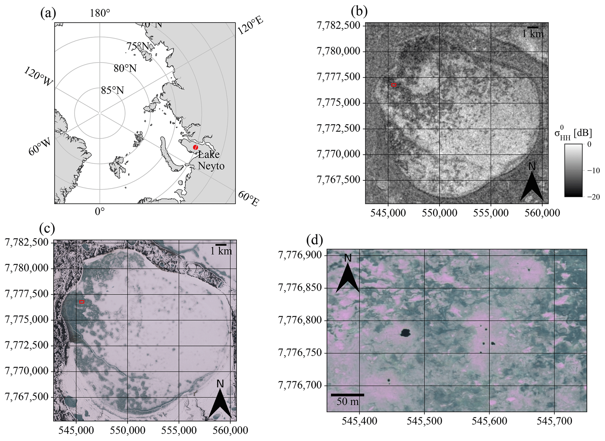
Figure 1 Location of Lake Neyto and visual comparison of potential signs of gas emissions in satellite data. (a) Location of Lake Neyto in the Arctic. (b) Backscatter anomalies are visible as clusters of low backscatter surrounded by regions of much higher backscatter in a Sentinel-1 EW HH-polarised acquisition from 16 May 2016. (c) Regions where snow seems to have melted earlier that appear similar to the regions of backscatter anomalies in the Sentinel-1 image can be seen in a Sentinel-2 true-colour composite from 21 May 2016. (d) Zoomed-in view of a WorldView-2 true-colour composite from 22 May 2016, where holes in the ice are visible as dark spots surrounded by very bright ice. The red rectangle in (b) and (c) indicates the region of the zoomed-in view in (d). Coordinate reference system (CRS): (a) WGS 84 / Arctic Polar Stereographic, (b)–(d) WGS 84 / UTM zone 42N.

3 Data

3.1 Sentinel-1 synthetic aperture radar data

The two polar-orbiting satellites Sentinel-1A and Sentinel-1B are part of the European Union's (EU) Copernicus programme. They were launched into orbit in April 2014 and in April 2016. The identical SAR sensor on both satellites, called C-SAR, can be operated in different acquisition and polarisation modes at a centre frequency of 5.405 GHz. The acquisition modes differ from each other in terms of spatial resolution and swath width. Data can be acquired in either single co-polarised or dual co-polarised plus cross-polarised channels (European Space Agency, 2012).

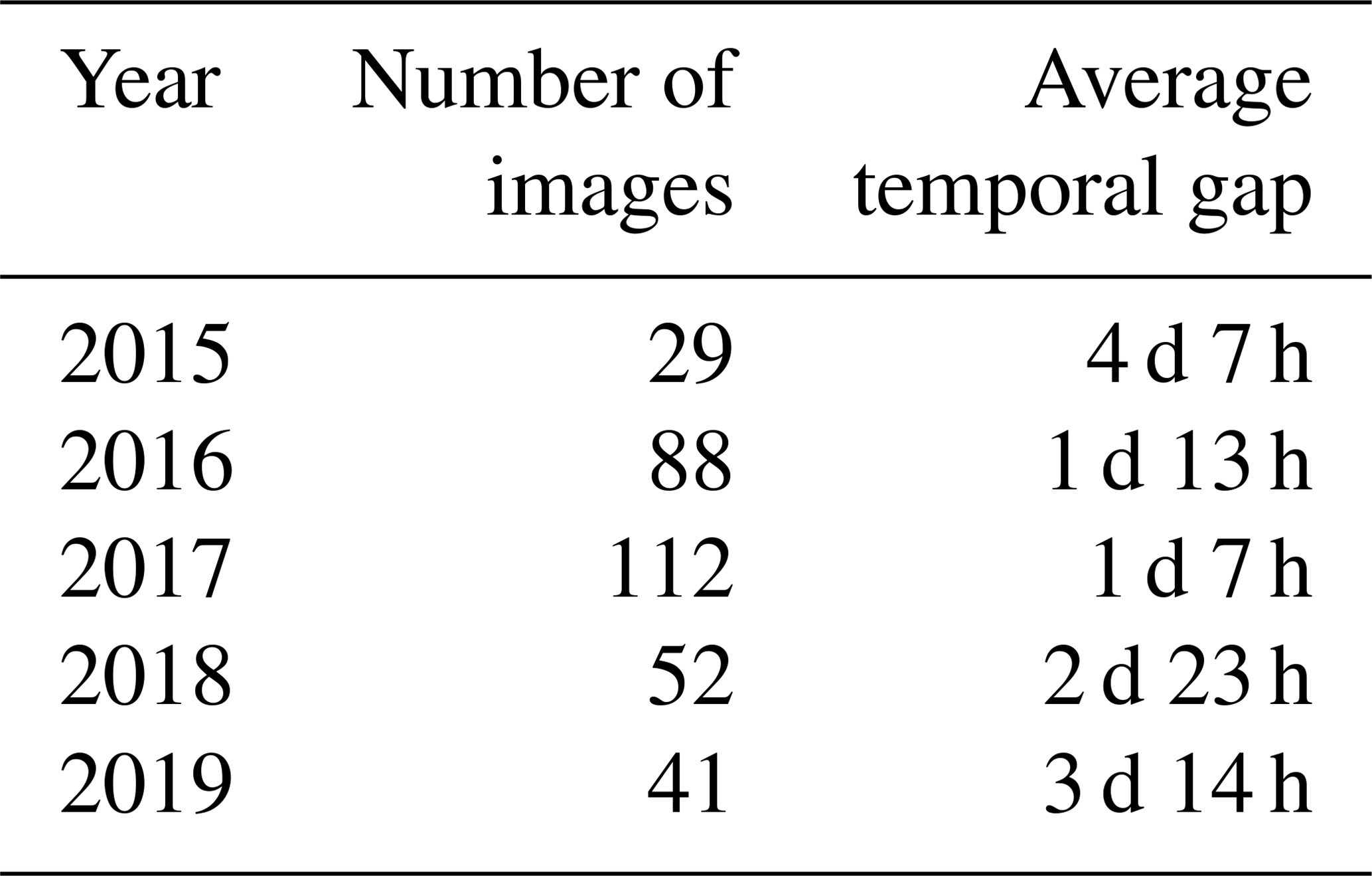
The default operating mode over land is the Interferometric Wide (IW) swath mode with vertical–vertical (VV) and vertical–horizontal (VH) dual-polarised acquisitions (European Space Agency, 2012). However, acquisitions over Lake Neyto are most frequently taken in Extra Wide (EW) swath mode with horizontal–horizontal (HH) and horizontal–vertical (HV) dual polarisation. EW data are acquired at larger swath widths compared to IW data, but IW data have a finer spatial resolution than EW data. Commonly used pixel spacing after the pre-processing steps is 40 m in EW mode and 10 m in IW mode. The number of EW acquisitions over Lake Neyto is significantly larger (Pointner and Bartsch, 2020), and no acquisitions in IW mode were taken in 2016. Hence, the primary SAR data for our analyses were Sentinel-1 EW data with both HH and HV polarisation channels. Table 1 shows the years of data, the number of Sentinel-1 EW images and the average temporal gap between the image acquisitions in the years concerned.

Table 1 Years of Sentinel-1 EW data and associated numbers of images and average temporal gaps.

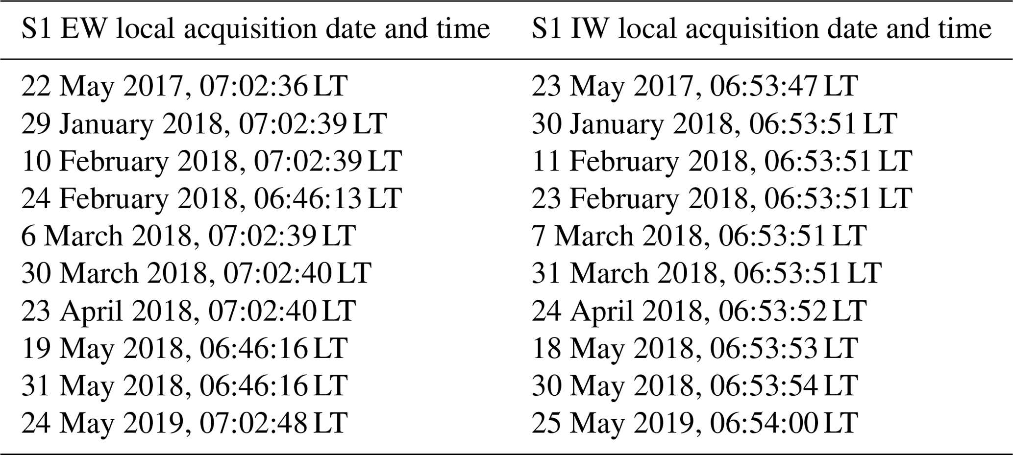
We used IW data for validation purposes and visual comparisons. A validation was carried out that compared classified anomalies from EW images and IW images that were acquired on consecutive dates (for details see Sect. 4.3). The local acquisition dates and times (LT) of these validation data are shown in Table 2.

Table 2 Local acquisition dates and times of pairs of Sentinel-1 EW and IW scenes used for validation.

Lists of the used scenes including the mean projected local incidence angle over the lake, acquisition times in local time and coordinated universal time (UTC), and an indicator showing if the scenes were assembled due to slicing (see Sect. 4.1.1) are provided in the Supplement (Tables S1–S4) to this article in CSV format. “S1__scene_metadata_list_Sentinel1_EW_main.csv” contains a list of the main Sentinel-1 EW data (342 scenes) used in this study. “S2__scene_metadata_list_ Sentinel1_EW_lake_masks.csv” and “S3__scene_metadata_ list_Sentinel1_EW_shelf_masks.csv” contain lists of the Sentinel-1 EW data used for calculating lake masks (5 scenes) and shelf masks (5 scenes), respectively (see Sect. 4.2.1 for details). “S4__scene_ metadata_list_Sentinel1_IW.csv” contains a list of all Sentinel-1 IW data used for the validation (10 scenes). “S5__scene_metadata_list_other_sensors.csv” contains a similar list for the other satellite data (4 scenes in total) used in this study, which are described in the following paragraphs.

3.2 WorldView-2 very high resolution optical data

The WorldView-2 satellite was launched in October 2009 and is operated by Maxar Technologies (formerly DigitalGlobe). It was the first commercial satellite to collect data at a very high spatial resolution in eight spectral bands. WorldView-2 data include a panchromatic band covering the wavelength range from 450 to 800 nm. The spatial resolution is 1.84 m for the multispectral bands and 0.46 m for the panchromatic band (Padwick et al., 2010). For this study, 100 km² of orthorectified WorldView-2 imagery (eight multispectral bands plus one panchromatic band) from 22 May 2016 covering approximately half of the surface area of Lake Neyto was available.

3.3 ALOS PALSAR-2 fully polarised SAR data

The PALSAR-2 sensor on board the Advanced Land Observing Satellite-2 (ALOS-2) is the successor to the PALSAR instrument on ALOS and operates at slightly varying centre frequencies of between 1.237 and 1.279 GHz (Kankaku et al., 2013). ALOS-2 was launched in May 2014 and is operated by the Japan Aerospace Exploration Agency (JAXA). Similarly to Sentinel-1, PALSAR-2 can be operated in different imaging modes with varying ground resolutions and swath widths, but it is able to acquire data in single-polarisation (HH, HV, VH or VV), dual-polarisation (HH + HV or VV + VH) and full-polarisation (HH + HV + VH + VV) modes (Kankaku et al., 2013). In this study, we used an ALOS PALSAR-2 fully (quad-)polarised scene in High-Sensitive Stripmap mode from 18 April 2015, which was acquired at a swath width of 50 km and a ground resolution of approximately 6 m (Kankaku et al., 2013) for polarimetric analyses to infer possible scattering mechanisms for anomaly regions and regular floating lake ice.

3.4 Sentinel-2 medium resolution optical data

Sentinel-2A and Sentinel-2B are also part of the EU's Copernicus programme and were launched into orbit in June 2015 and March 2017, respectively. The two satellites carry an identical multispectral instrument which acquires data in 12 spectral bands in the optical, near-infrared and short-wave infrared range (Drusch et al., 2012). The spatial resolution varies between bands and is 10, 20 or 60 m. The red, green and blue bands have a spatial resolution of 10 m. In this study, Sentinel-2 true-colour composites based on the 10 m resolution bands were used for visual interpretations.

3.5 Landsat 8 brightness temperature and surface reflectance

Landsat 8 is the latest satellite of the Landsat satellite series that have been continuously providing multispectral data of the earth's land surface since 1972. Landsat 8 was launched in February 2013 and carries the Operational Land Imager (OLI) and the Thermal Infrared Sensor (TIRS) instruments. OLI acquires data in eight spectral bands in the optical, near-infrared and short-wave infrared range at a 30 m spatial resolution and in one panchromatic band at a 15 m spatial resolution (Roy et al., 2014). TIRS collects data in two spectral bands in the thermal infrared range at a 100 m spatial resolution (Roy et al., 2014). We used a true-colour composite of surface reflectance and the band-10 brightness temperature of a Landsat 8 scene of Lake Neyto acquired on 6 April 2015 for visual comparisons to the SAR data.

3.6 ERA5 2 m air temperature

ERA5 is the fifth generation of European Centre for Medium-Range Weather Forecasts (ECMWF) global climate and weather reanalysis. Reanalysis uses combined model data and observations on a global scale to derive a complete and consistent dataset (Hersbach et al., 2018). The ERA5 product of hourly data on single levels from 1979 to the present contains hourly estimates for a variety of atmospheric, ocean-wave and land-surface parameters on a regular latitude–longitude grid of 0.25^∘ (Hersbach et al., 2018). In this study, we used the “2 m temperature” variable, which represents near-surface air temperature, for a comparison to the temporal dynamics of the backscatter anomalies. The 2 m temperature data for the nearest grid point to Lake Neyto (70^∘ N, 70.25^∘ E) were therefore aggregated to daily minima and maxima using the cdstoolbox.geo.extract_point and cdstoolbox.climate.daily_min and cdstoolbox.climate.daily_max methods of the Python application programming interface (API) of the Copernicus Climate Change Service (C3S) Climate Data Store (CDS). The data were subsequently downloaded and converted to degrees Celsius.

4 Methods

4.1 Pre-processing of satellite data

4.1.1 Pre-processing of Sentinel-1 SAR data

The majority of pre-processing steps for Sentinel-1 EW and IW data were conducted with the graph processing tool (gpt) of the Sentinel Application Platform (SNAP) toolbox (Zuhlke et al., 2015). Some products have been sliced directly over the lake. In these cases, the slice-assembly operator was applied to those products in the gpt as the first processing step. Products to which this operator was applied are indicated in Tables S1–S4. In the following, the applied operators within the gpt were subsetting, radiometric calibration, thermal noise removal and terrain correction using the ArcticDEM version 3.0 (Porter et al., 2018). The well-known-text (WKT) representation of the subset extent in World Geodetic System 84 (WGS 84) geographical coordinates is POLYGON ((69.2277 69.7650, 70.9744 69.7650, 70.9744 70.3610, 69.2277 70.3610, 69.2277 69.7650, 69.2277 69.7650)). After these steps, the data were converted to decibels (dB) and incidence angle normalisation was performed. The incidence angle normalisation methodology used here is described in Pointner et al. (2019) and uses empirically derived normalisation functions in the form of second-degree polynomials to normalise backscatter in decibels to a common reference incidence angle of 30^∘. The normalisation function can be written as

$$\begin{array}{}\text{(1)}& {\mathit{\sigma }}_{\mathrm{norm}}^{\mathrm{0}}\left(\mathit{\theta }\right)\left[\mathrm{dB}\right]=a\cdot {\mathit{\theta }}^{\mathrm{2}}+b\cdot \mathit{\theta }+c,\end{array}$$

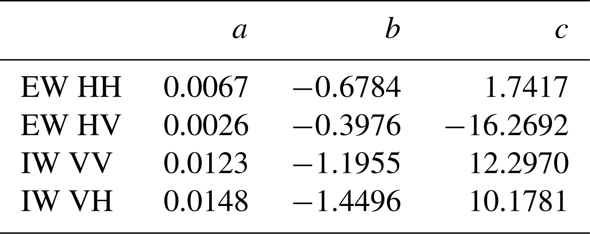
where ${\mathit{\sigma }}_{\mathrm{norm}}^{\mathrm{0}}\left(\mathit{\theta }\right)$ is the normalisation function; θ is the local projected incidence angle; and a, b and c are the polynomial coefficients. The polynomial coefficients in Eq. (1) used for the incidence angle normalisation with respect to the sensor mode and polarisation are given in Table 3.

Table 3 Polynomial coefficients used for the incidence angle normalisation with respect to the sensor mode and polarisation.

Based on these coefficients, the final normalisation to the reference incidence angle of 30^∘ was applied using (Pointner et al., 2019)

$$\begin{array}{}\text{(2)}& {\mathit{\sigma }}^{\mathrm{0}}\left(\mathrm{30}\right)={\mathit{\sigma }}^{\mathrm{0}}\left(\mathit{\theta }\right)-\left({\mathit{\sigma }}_{\mathrm{norm}}^{\mathrm{0}}\right(\mathit{\theta })-{\mathit{\sigma }}_{\mathrm{norm}}^{\mathrm{0}}(\mathrm{30}\left)\right),\end{array}$$

where σ⁰(30) is the backscatter coefficient normalised to 30^∘, σ⁰(θ) is the backscatter coefficient before normalisation, ${\mathit{\sigma }}_{\mathrm{norm}}^{\mathrm{0}}\left(\mathit{\theta }\right)$ is the value of the normalisation function at the incidence angle concerned and ${\mathit{\sigma }}_{\mathrm{norm}}^{\mathrm{0}}\left(\mathrm{30}\right)$ is the value of the normalisation function at 30^∘.

All steps were applied to both polarisation channels (HH and HV for EW mode, VV and VH for IW mode). Outputs were images of normalised backscatter coefficient σ⁰.

4.1.2 Pre-processing of optical imagery

We calibrated the WorldView-2 data from 22 May 2016 to top-of-atmosphere (TOA) reflectance following the methodology given by Updike and Comp (2010) and applied pan-sharpening from the Geospatial Data Abstraction Library (GDAL) command line utilities (version 2.2.4) which is based on the Brovey method (GDAL/OGR contributors, 2020) using all available bands.

Sentinel-2 data were downloaded in level-1C (L1C) format and directly used for visual comparisons.

4.1.3 Polarimetric processing of ALOS PALSAR-2 fully polarised SAR data

From the fully polarised ALOS PALSAR-2 data in High-Sensitive Stripmap mode acquired on 18 April 2015, we deduced two polarimetric products in order to infer scattering properties of regular floating lake ice and anomaly regions. Firstly, we calculated the coherency matrix T₃ (Lee and Pottier, 2009), of which the first element T₁₁ has been shown to relate to surface scattering and correlate with the area of gas bubbles trapped in lake ice and methane flux estimates of ice-covered lakes in Alaska (Engram et al., 2020, 2013). The calculations were performed in SNAP, and the processing steps were radiometric calibration, calculation of T₃ (Lee and Pottier, 2009), polarimetric speckle filtering using the refined Lee filter (Lee et al., 2008), terrain correction using the ArcticDEM and spatial subsetting. Secondly, we performed an unsupervised polarimetric classification using the method proposed by Cloude and Pottier (1997), which can allow for a detailed identification of scattering mechanisms. In comparison with the calculation of T₃, the workflow was essentially the same, with the only difference being that between the polarimetric speckle filtering and terrain correction steps, the polarimetric classification was computed. The classification itself consists of two main steps. The first step is the polarimetric decomposition and extraction of entropy (H) and alpha (α) parameters (Cloude and Pottier, 1997; Lee and Pottier, 2009), and the second step is the classification based on nine discrete regions in the H-α plane (Cloude and Pottier, 1997). Each of these regions indicates the dominant scattering mechanism in the resolution cell concerned (Cloude and Pottier, 1997). The output pixel values from SNAP did not correspond to the zone designations in Cloude and Pottier (1997) and Lee and Pottier (2009); i.e. regions in the H-α plane were labelled by different numbers comparing between the SNAP documentation and Cloude and Pottier (1997) and Lee and Pottier (2009). Thus, we reclassified the output to match the designations of Cloude and Pottier (1997) and Lee and Pottier (2009).

4.2 Classification and detection methods

4.2.1 Classification of backscatter anomalies from Sentinel-1 data

The method to classify backscatter anomalies (clusters of unusually low backscatter) in Sentinel-1 SAR images was briefly outlined in Pointner and Bartsch (2020) but is given here in greater detail. The input for the classification algorithm is pre-processed Sentinel-1 images of σ⁰ in decibels after incidence angle normalisation. All steps described in the following were identically performed on both polarisation channels. The most important software packages used for the classification were the Python packages scikit-image (skimage) version 0.15.0 (van der Walt et al., 2014), GDAL version 2.2.4 (GDAL/OGR contributors, 2020), SciPy version 1.1.0 (Virtanen et al., 2020) and NumPy version 1.15.1 (Harris et al., 2020).

As a first step, areas outside the lake and the shelf area of the lake, where ground-fast ice is assumed, were masked. We deduced lake masks from late-autumn Sentinel-1 EW imagery and shelf masks from winter Sentinel-1 EW imagery through binary classification for each year separately. For the extraction of the lake masks, we used Otsu thresholding (Otsu, 1979) on the HH-polarisation band (σ⁰ in dB) implemented in scikit-image (skimage.filters.threshold_otsu, default parameters) of the late-autumn acquisitions. Here, no incidence angle normalisation was applied, as the incidence angle range over the lake was small and the backscatter values were only used to create the masks and were not compared to those of other acquisitions. After thresholding, we used the method scipy.ndimage.morphology.binary_fill_ holes (default parameters) to fill holes in the classification result, polygonised the result using gdal_polygonize.py (default parameters) and extracted the polygon of Lake Neyto. Images used for the classification were cropped to the extent of the lake masks. For the shelf masks, we selected the latest date where clusters of low-backscatter pixels on assumed floating ice were not spatially connected to the shelf zone, where ground-fast lake ice was assumed. The shelf masks were computed through a binary classification on the HH-polarisation band using incidence-angle-dependent thresholding as described by Pointner et al. (2019) and extraction of all areas that were classified as ground-fast lake ice and connected to the lake outline. Additionally, binary dilation (skimage.morphology.dilation with selem=skimage.morphology.disk(3), otherwise default parameters) was applied to this shelf mask to exclude areas that may be affected by late grounding of the lake ice in late winter or spring from the classification.

After masking, pixel values were re-scaled from decibels to the interval from −1 to 1 using skimage.exposure.rescale_intensity (out_range=(-1,1); in_range=(-40,0) in the case of co-polarisation; in_range=(-50,-10) in the case of cross polarisation), as required by the image processing algorithms applied in the following. The main image processing steps were bilateral filtering to reduce noise in the images, local auto-levelling to balance out the unevenly distributed backscatter level across the lake, and Yen thresholding (Yen et al., 1995) to automatically classify the images into the two categories for floating lake ice “low-backscatter anomalies” (positive class) and “high backscatter from regular floating lake ice” (negative class).

For the bilateral filtering, we used skimage.filters.rank.mean_bilateral (selem=skimage.morphology.square(5); s0=20 in the case of EW; s0=150 in the case of IW; s1=150 in both cases). For the local auto-levelling, we defined specific kernels as NumPy arrays. In the case of EW data, numpy.ones([51,int(image.shape[1]/4)]) was used. In the case of IW data, numpy.ones([204,int(image.shape[1]/4)]) was used. Here, the shape of the image (image.shape) had been defined by the cropping of the pre-processed images by the lake masks. These kernels were then rotated using scipy.ndimage.interpolation.rotate (angle=45, otherwise default parameters) by 45^∘, as the largest backscatter gradient seemed to often occur from northwest to southeast of the lake in many images. The local auto-levelling itself was then performed using skimage.filters.rank.autolevel_percentile (with the defined kernel and p0=0 and p1=1). Although using 0 and 1 as percentiles, we encountered different behaviour of this method regarding the treatment of the no-data mask when compared to the method skimage.filters.rank.autolevel, and thus skimage.filters.rank.autolevel_percentile was preferred. Yen thresholding was in the following applied to the imagery using skimage.filters.threshold_yen with default parameters.

The output of these steps were two classified binary images: one for the co-polarised channel (HH in EW mode, VV in IW mode) and one for the cross-polarised channel (HV in EW mode, VH in IW mode). The bilateral mean filter was chosen to handle noise with the aim of binary classification in mind, as opposed to a conventional speckle filter.

We applied a logical AND operator (numpy.logical_and, default parameters) to these two images to keep only pixels that belong to the class of backscatter anomalies in the outcome of both polarisation channels. Since we had no in situ data available (see Sect. 4.3), we tried to use conservative settings wherever possible. In order to mitigate potential remaining noise even further, we removed connected components (4-neighbourhood) smaller than the size of 9 Sentinel-1 EW pixels from the final classification result (skimage.morphology.remove_small_objects).

Since Yen thresholding determines the threshold for the binary classification automatically, it is not applicable if backscatter anomalies are not present in the image. Since the mapping of clusters should be automatic, we needed to include a test of whether anomalies were apparent in the images. Our approach again utilises the dual-polarisation capability of Sentinel-1 and tests the similarity between classification outcomes of the two polarisation channels using Cohen's kappa score κ (Cohen, 1960). Only if κ was above 0.2 (class “fair agreement” according to Landis and Koch, 1977), was the final classification produced as described above. If κ was below 0.2, all pixels in the image were assigned to the negative class.

The classification method was especially designed to map anomalies in late-winter and spring images. A considerable ice thickness is required to resist wind forces without breaking on large lakes, and SAR imagery of lake ice acquired during early periods of ice formation can exhibit features of fracturing, movement or refreezing (Duguay and Pietroniro, 2005). Our algorithm may classify such features in autumn or early-winter images incorrectly as the targeted anomalies. To prevent this, we restricted time series analyses to imagery acquired after 1 January in all years concerned.

4.2.2 Detection and mapping of holes in lake ice from WorldView-2 data

For the automated detection of open holes in the ice from the WorldView-2 acquisition, we used a blob detector from scikit-image which uses the Laplacian of Gaussian (LoG) filter (van der Walt et al., 2014). The term blob stands for “binary large object”, and the holes in the ice are considered blobs here. The intention behind using this approach was to automatically map dark round spots in the imagery characterised by high contrast to the surrounding regions in a reproducible manner. The blob detector is a method to be applied to greyscale imagery. We used the green band as the input as it allowed for the best separation between holes and surface features that we did not interpret as holes but could have been confused with holes by the blob-detection algorithm. The detector works by successively convolving the image with LoG kernels of increasing standard deviation and stacking up the responses in a cuboid. Detected blobs are local maxima in the cuboid that are filtered using an intensity threshold on the maxima. Again, we tried to be very cautious when selecting this threshold to only detect dark round spots characterised by significant contrast to the surrounding pixels that are most likely holes in the lake ice. The method skimage.feature.blob_log (min_sigma=0.69, max_sigma=10, num_sigma=200, threshold=0.187) was used on the negative of the green-band pan-sharpened TOA reflectance image. Figure 2 gives an example of what we interpreted as holes and what features we sought to prevent from being detected as holes. Figure 2a shows a true-colour composite, and Fig. 2b shows an associated spectral profile. The red line in Fig. 2a indicates the pixels used for plotting the profile in Fig. 2b (lower left to upper right). Two main minima can be identified. The left minimum was interpreted as a hole that should be detected by the algorithm (and also the other two dark spots in the lower left of the image), while the right minimum was not considered a hole and it should not be detected by the algorithm. In most bands, the contrast between both minima and the surrounding pixels is similar, while the smallest contrast for the right minimum is observed in the green band.

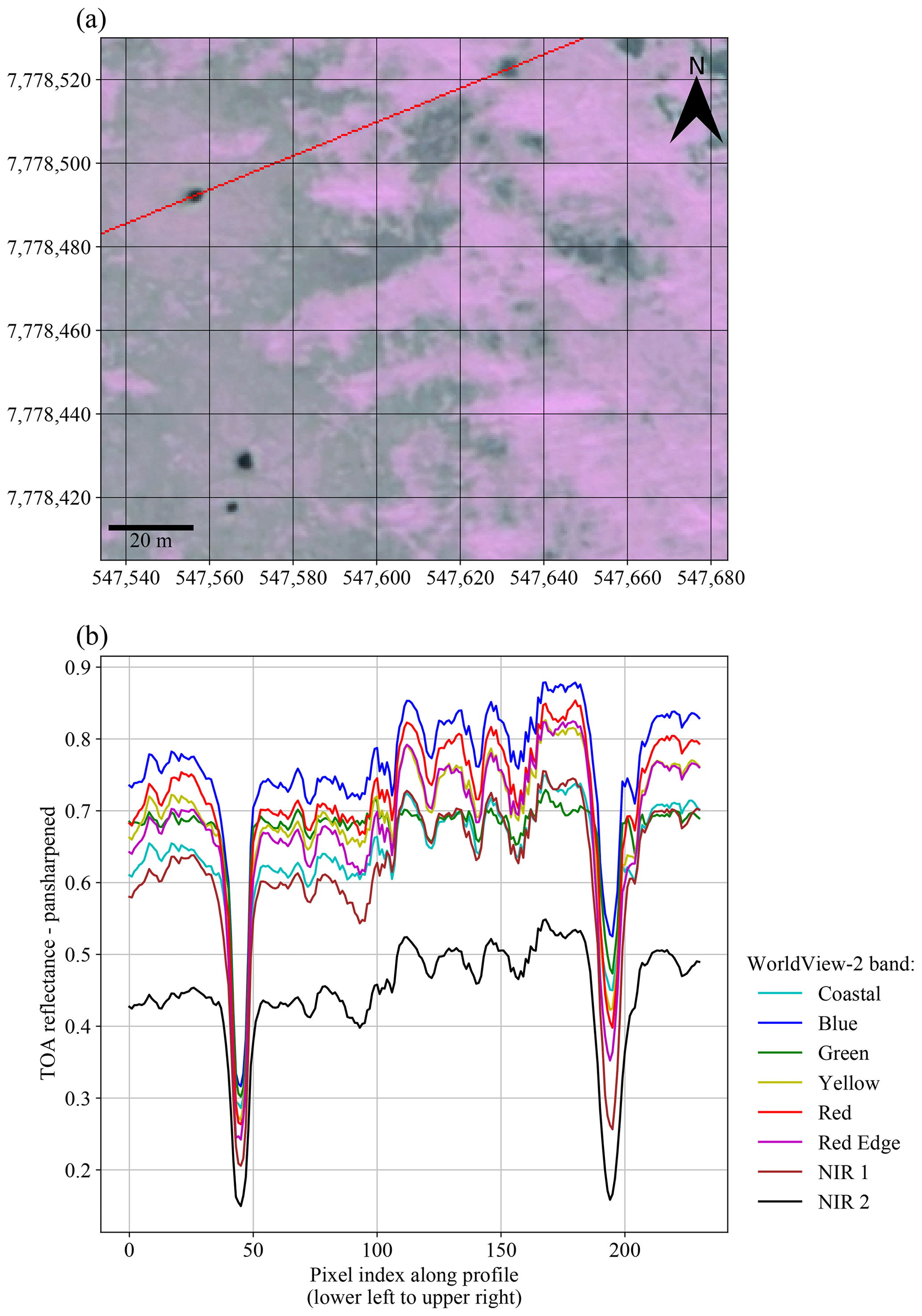
Figure 2 Examples of features in WorldView-2 imagery acquired on 22 May 2016 and associated spectral profile. (a) WorldView-2 true-colour composite with red line indicating the pixels used for plotting the profile (CRS: WGS 84 / UTM zone 42N). (b) Spectral profile indicating variations between contrast for the two main minima. The left main minimum was considered a hole that should be detected, while the right minimum was not considered a hole, and its detection should be avoided.

The outputs of the algorithm are the coordinates of the blob centres and the corresponding radii approximated from the standard deviation of the LoG kernel that detected the blob concerned. In order to estimate hole areas, we performed a binary classification based on a marker-based watershed segmentation using the blob-detection results to classify all pixels belonging to the holes. Markers for the hole class were set on single pixels on which the centres of detected blobs were located. Markers for the background class were set on pixels with pan-sharpened TOA reflectance larger than 0.45. The marker image was defined with the same size as the original image, with value 1 for the hole markers, value 2 for the background class and value 0 elsewhere. After the definition of the markers, the watershed segmentation (skimage.segmentation.watershed, default parameters) was applied using the original image and the marker image, and individual hole objects were extracted and vectorised. In rare cases, the watershed segmentation produced unsatisfactory results by clearly overflowing the area of the expected hole. To handle these false classifications, we excluded all hole polygons larger than 300 m² from further analysis (the largest open holes formed by subcap seepage in Walter Anthony et al., 2012, were reported to be approximately 300 m² in area).

4.3 Validation of Sentinel-1 classification methodology

No in situ data were available for Lake Neyto to validate the classification of anomaly regions from Sentinel-1 data directly. The remoteness of the area and the absence of transportation infrastructure largely impedes in situ data collection. More strikingly, it is likely that parts of the regions of backscatter anomalies on the lake are characterised by very thin ice, which would pose a direct threat to human safety if in situ data collection on the lake ice was attempted. Ice only a few centimetres thick was also reported by the Yamal-Nenets on Lake Yambuto in mid-march 2017, where ice thickness at that time is usually more than 1 m (Pointner et al., 2019).

Due to the lack of reference data collected at site, we propose a comparison of classification results from EW data (HH and HV polarisation) and IW (VV and VH polarisation) data acquired on consecutive dates. The anomalies are visible in all polarisation channels, and their extent is expected to be similar on consecutive dates in the two modes. In all winters and springs with acquisitions, we could identify 10 points in time when Lake Neyto was observed in the two modes on successive days (Table 2). For each of the dates, we re-sampled (nearest neighbour) and re-projected the binary classification image from the IW mode (10 m pixel spacing) to the binary classification image from the EW mode (40 m pixel spacing) in order to be able to carry out pixel-based comparisons. Here, the classification on the EW data was assessed against the classification on the IW data that acted as a reference set.

Several metrics have been proposed to assess binary classification outcomes in the case of imbalanced classes (Chicco and Jurman, 2020). From the confusion matrix calculated from the EW and IW classification results, we estimate the total number of pixels in the negative class (regular floating lake ice) to be about 1 order of magnitude larger than the total number of pixels in the positive class (anomalies) in the validation dataset (Table 2), so class imbalance is clearly the case here and simple accuracy measures should be avoided (Chicco and Jurman, 2020). We faced a similar situation of imbalance when looking at the number of pixels classified positively over time; i.e. there is a significant difference between the number of pixels classified positively in February and the number of pixels classified positively in May, for example. So, we argue that averaging metrics over the 10 points in time (Table 2) cannot be representative for the classification method either. We propose to calculate binary metrics which are suitable in the case of imbalanced classes on all classified pixels in the validation dataset, together. Specifically, we calculated F1 scores (Dice, 1945; Sørensen, 1948), the Matthews correlation coefficient (Matthews, 1975) and Cohen's kappa coefficient κ (Cohen, 1960). F1 scores are generally calculated per class. We give two versions of F1 scores here, one being the F1-score binary, which is calculated for the positive class (anomalies) only, and one being the F1-score macro, which is the average of the F1 scores of the positive and negative class.

In order to compare backscatter levels among modes and polarisation channels, we also used the data from this validation dataset because of the short time interval between acquisitions in the two modes. We calculated mean σ⁰ per class and date, took the difference between the means per class for each acquisition date, and calculated the mean of these differences over time. Further, we calculated the mean σ⁰ for the positive class on single dates and averaged it over time. All calculations were performed separately for each polarisation channel.

4.4 Summary of the most important methodological steps

A flow chart depicting the most important processing, selection and analysis steps associated with Sentinel-1 and WorldView-2 data is shown in Fig. 3. Sentinel-1 EW and IW data were both pre-processed and classified using a similar methodology. Classification results of IW and EW data acquired on consecutive dates (Table 2) were used to calculate validation metrics. Polygons of detected holes deduced from the blob detection and subsequent watershed segmentation on the green band of the pan-sharpened WorldView-2 image acquired on 22 May 2016 were used to calculate statistics of the hole area. Detected locations of holes as produced by the blob-detection algorithm were visually and quantitatively compared to single Sentinel-1 EW acquisitions and associated anomaly classification results from 16 May and 7 April 2016.

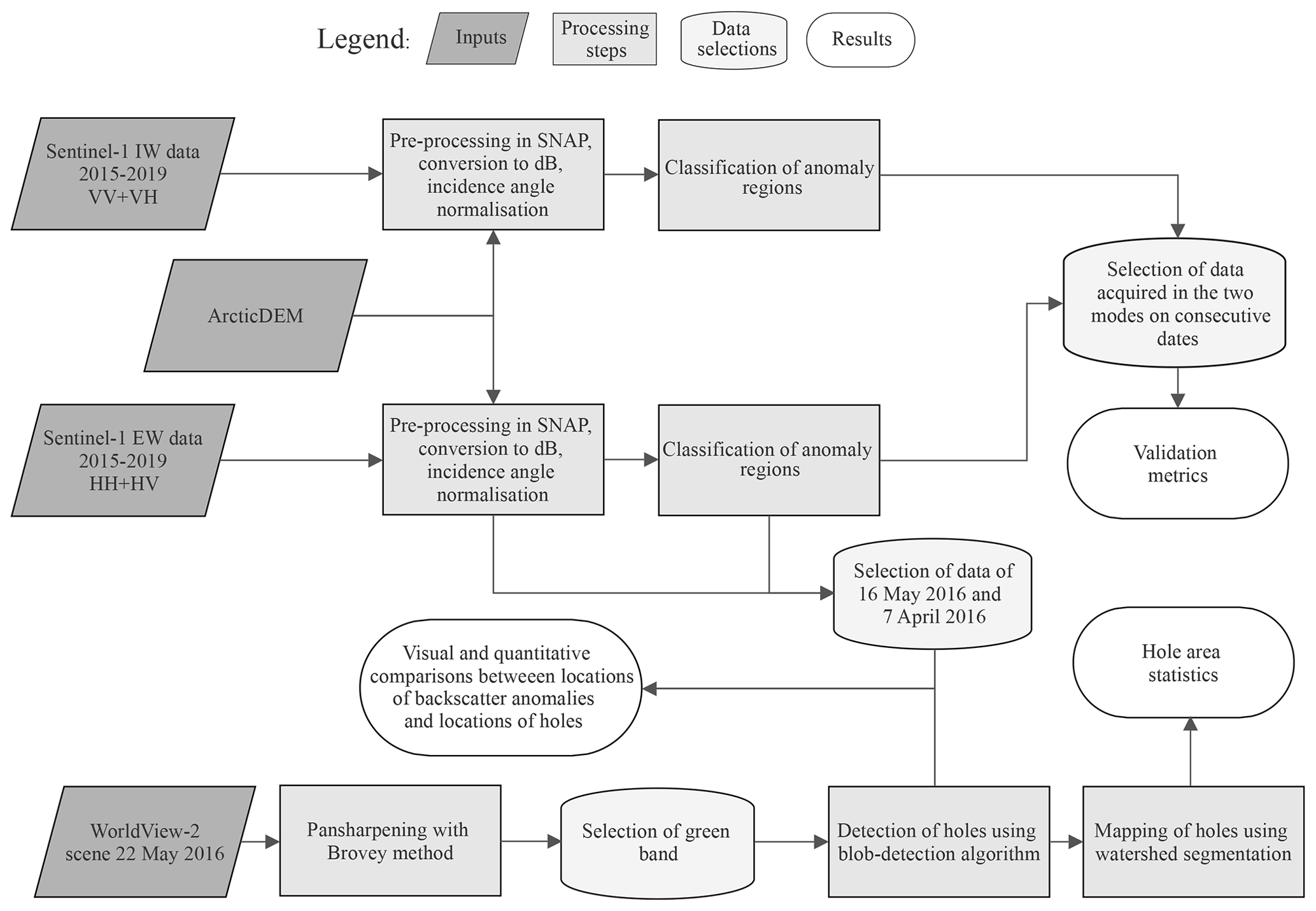
Figure 3 Workflow of main processing, selection and analysis steps associated with Sentinel-1 and WorldView-2 imagery in this study.

5 Results

An example of classification results from Sentinel-1 EW and IW imagery acquired on consecutive dates is given in Fig. 4 (HH-polarisation and VV-polarisation bands are shown in Fig. 4a and b, respectively). Anomalies are characterised by similar contrast and similar extents in the two acquisitions.

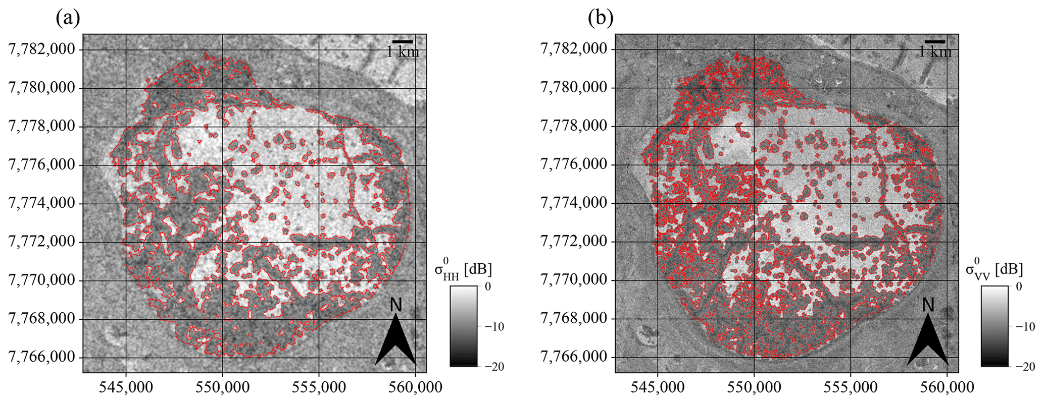
Figure 4 Example of Sentinel-1 EW and IW acquisitions taken 1 d apart and classification outcomes of backscatter anomalies. (a) Sentinel-1 EW HH-polarised acquisition from 24 May 2019. (b) Sentinel-1 IW VV-polarised acquisition from 25 May 2019. Red outlines represent polygon outlines from vectorised raster classification maps. CRS: WGS 84 / UTM zone 42N.

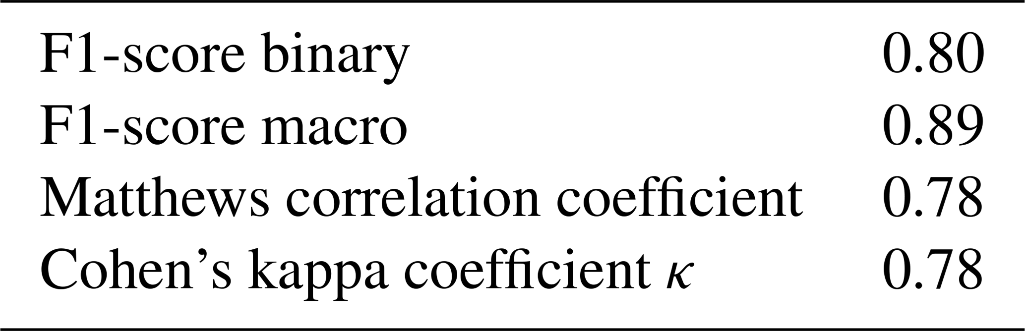
Table 4 shows the metrics calculated from the comparison between classifications from EW and IW modes in the validation set. κ and the Matthews correlation coefficient have the same value (0.78); the F1-score binary is slightly higher (0.80), and the value of the F1-score macro is 0.89.

Table 4 Metrics for the comparison between binary classifications of Sentinel-1 EW and Sentinel-1 IW acquisitions on consecutive days. A total of 10 pairs of EW and IW acquisitions were used.

As described in Sect. 4.3, the validation dataset consists of 10 pairs of Sentinel-1 images acquired in EW and IW modes on consecutive dates. Several statistics were calculated from the validation set to describe backscatter levels. Boxplots of σ⁰ for the positive class (anomalies) and negative class (regular floating lake ice) are shown in Fig. 5 for all polarisations and acquisition dates in the validation set. The temporal averages of the differences between mean σ⁰ of the positive and negative class on the single acquisition dates are 4.9 dB for the EW mode in HH polarisation, 6.0 dB for the EW mode in HV polarisation, 5.4 dB for the IW mode in VV polarisation and 7.2 dB for the IW mode in VH polarisation.

The temporal averages of mean σ⁰ of the positive class (anomalies) on single acquisition dates are −12.2 dB for the EW mode in HH polarisation, −25.9 dB for the EW mode in HV polarisation, −14.1 dB for the IW mode in VV polarisation and −25.4 dB for the IW mode in VH polarisation.

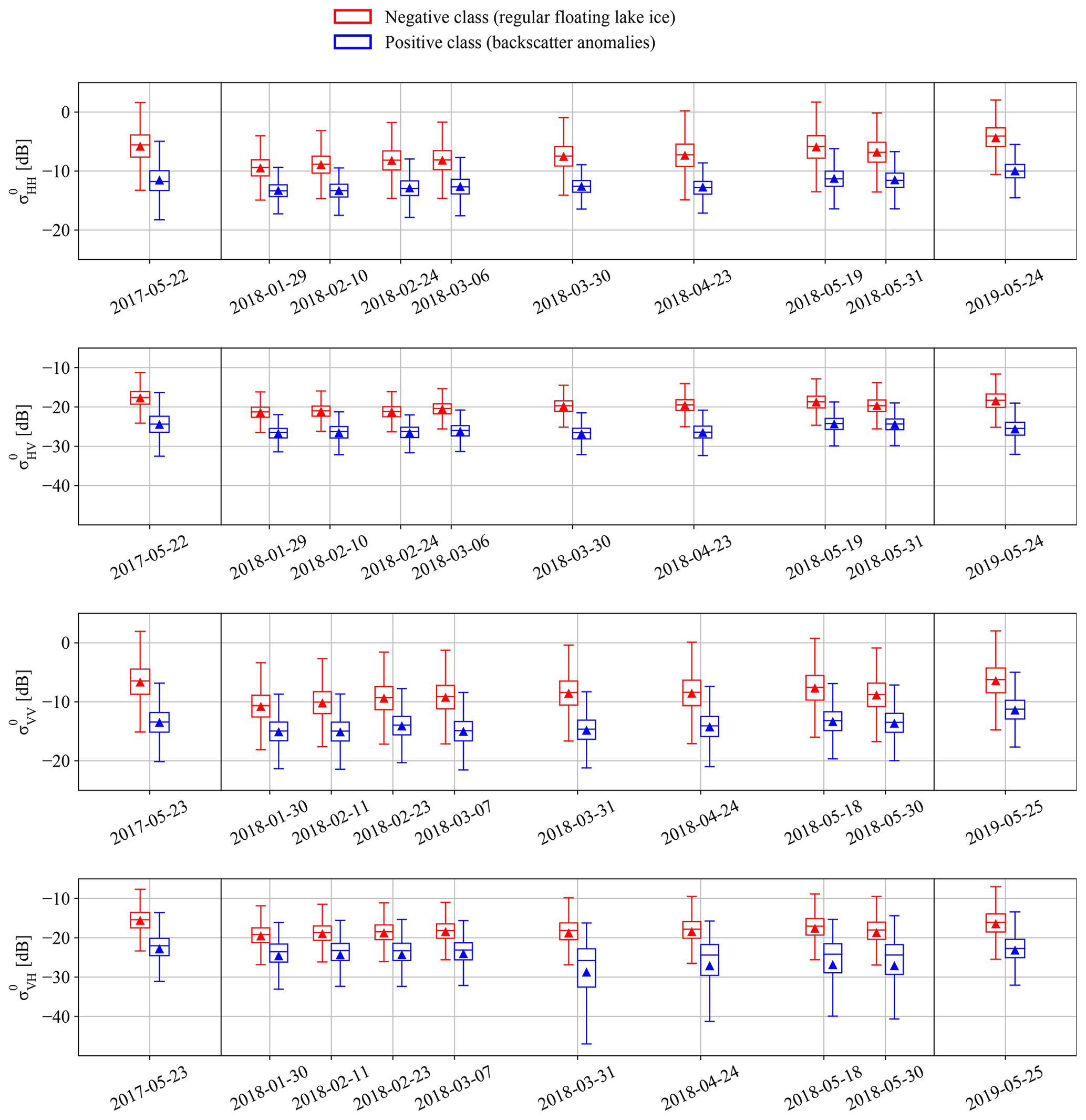
Figure 5 Boxplots of σ⁰ for the positive class (backscatter anomalies) and negative class (regular floating lake ice) for all polarisations (HH, HV, VV, VH) and all 10 acquisition dates in the validation set. The means are represented by triangles. Dates are given in the format year–month–day.

Figure 6a shows an example of detected holes in the lake ice of Lake Neyto on a true-colour composite of the WorldView-2 acquisition from 22 May 2016, and Fig. 6b shows examples of mapped holes from the watershed segmentation algorithm. Holes are clearly characterised by dark tones surrounded by regions of higher reflectance.

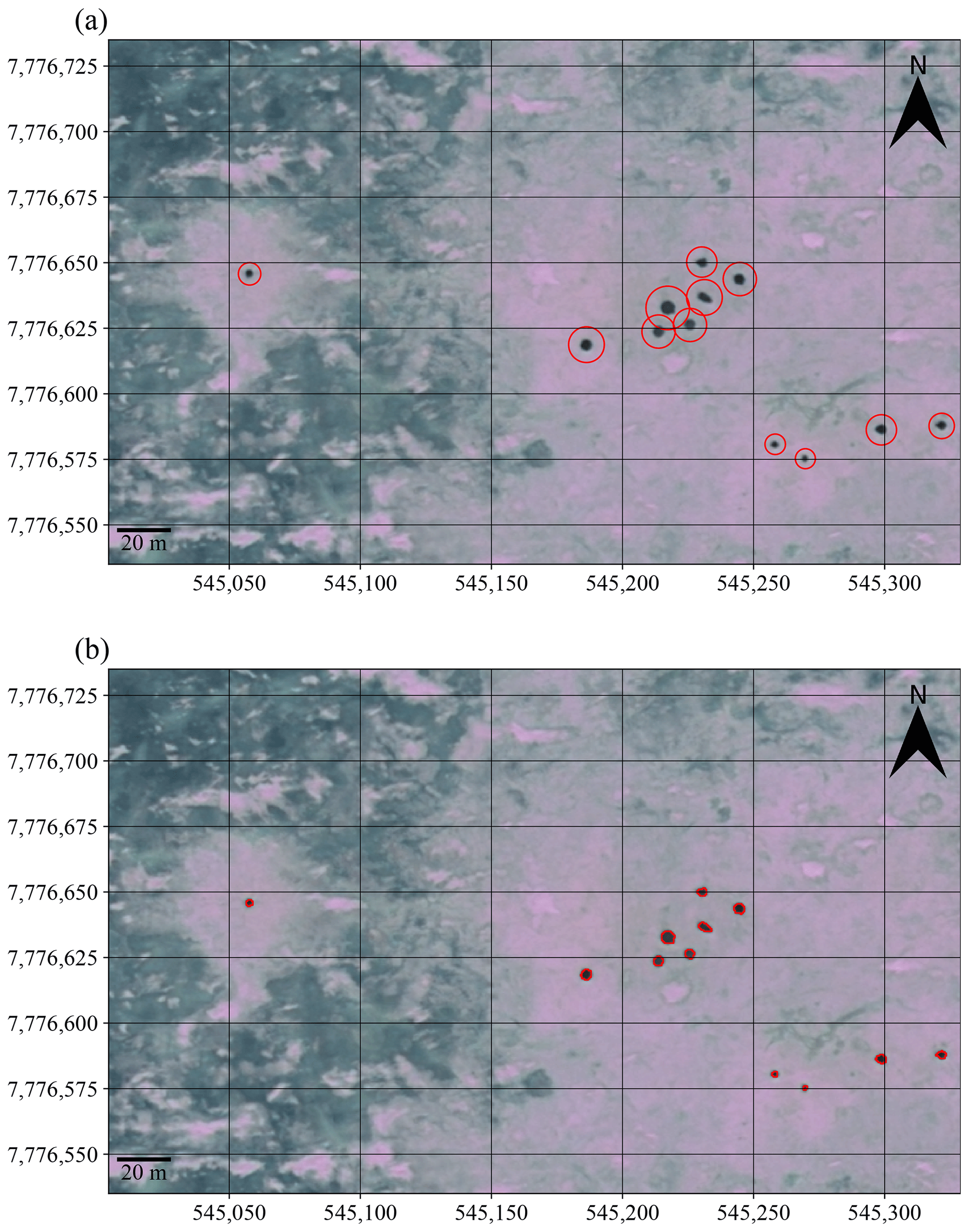
Figure 6 Examples of hole detection and classification results in lake ice of Lake Neyto on WorldView-2 true-colour composites acquired on 22 May 2016. (a) Examples of detected holes (red circles) from the blob-detection method. Radii of circles are scaled proportionally to the standard deviation of the LoG kernel that detected the respective blob, enlarged for the visualisation. (b) Mapped holes (red outlines) from the watershed segmentation method. CRS: WGS 84 / UTM zone 42N.

The blob-detection algorithm yielded locations of 718 holes. Out of 718 hole polygons deduced by using the watershed segmentation, 10 had to be excluded by the application of the area threshold (compare to Sect. 4.2.2). Figure 7 shows a histogram of hole areas from the remaining 708 hole polygons. The majority of holes are characterised by an area smaller than 5 m²; the median is 4.00 m². Few holes with areas larger than 50 m² were identified.

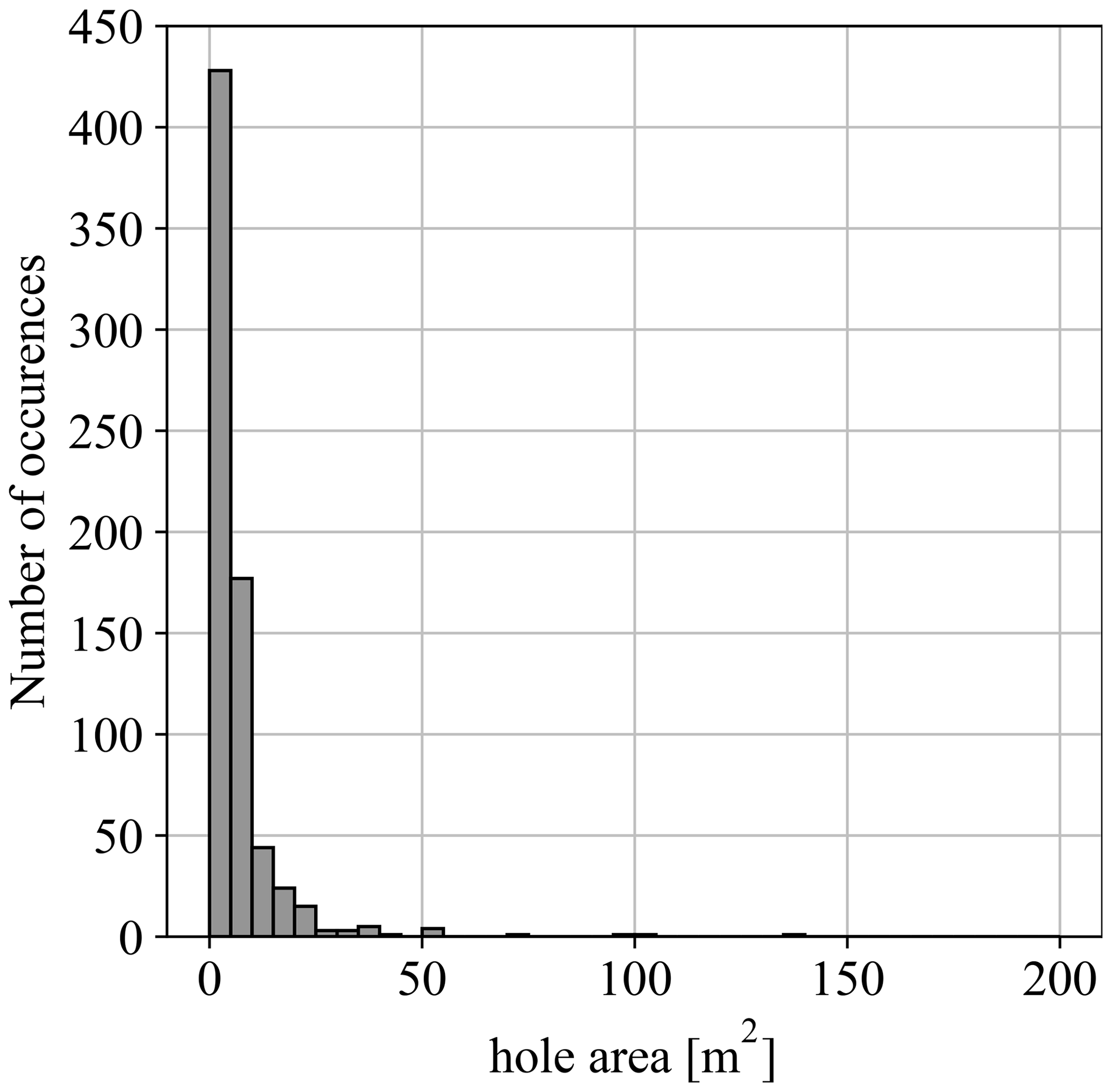
Figure 7 Histogram of hole areas from 708 hole polygons deduced from the watershed segmentation algorithm applied to the WorldView-2 image acquired on 22 May 2016.

The locations of the 718 detected holes (points, potential seep locations) from the WorldView-2 image acquired on 22 May 2016 and the Sentinel-1 HH-polarised image acquired on 16 May 2016 with the outlines of classified backscatter anomalies (polygons) are shown in Fig. 8. Of the 718 detected holes, 71 % lie within the polygons deduced from the Sentinel-1 classification result. The mean minimum distance between the points and the polygons is 38 m (if a point lies within a polygon, the distance is zero). The median distance of all points lying outside the polygons is 67 m.

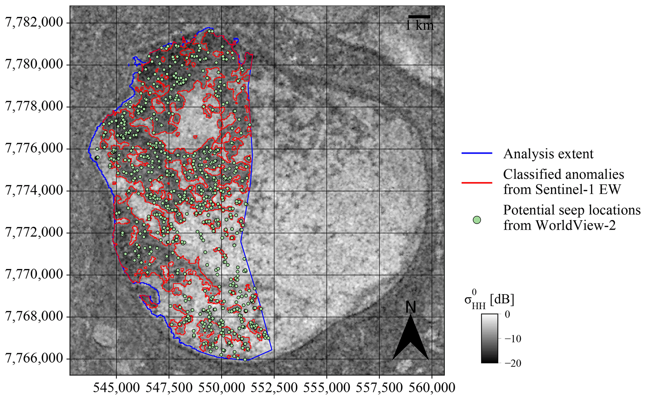
Figure 8 Comparison of detected holes (potential seep locations, green points) from WorldView-2 imagery acquired on 22 May 2016 and backscatter anomalies (red outlines) from a Sentinel-1 scene acquired on 16 May 2016 on top of the HH-polarisation band of the same scene. The blue outline shows the analysis extent that is determined by the extent of the WorldView-2 image and the lake and shelf masks. CRS: WGS 84 / UTM zone 42N.

Interesting spatial relationships can also be identified when comparing the locations of detected holes to Sentinel-1 imagery acquired earlier in the same year. Figure 9 shows the same locations of detected holes deduced from the WorldView-2 image acquired on 22 May 2016 as in Fig. 8 on top of a Sentinel-1 EW HH-polarised acquisition from 7 April 2016, taken more than a month earlier than the image in Fig. 8. A detailed view of the northwestern part of Lake Neyto is shown. A relationship between many locations of holes and backscatter anomalies with a smaller spatial extent can be identified. Maximum and minimum air temperatures on 22 May 2016 were 1.2 and −2.0 ^∘C, respectively, according to the ERA5 data (Hersbach et al., 2018). Apart from 1 April and 3 d from 22 to 24 April, maximum air temperature remained below 0 ^∘C until 16 May 2016 (Hersbach et al., 2018).

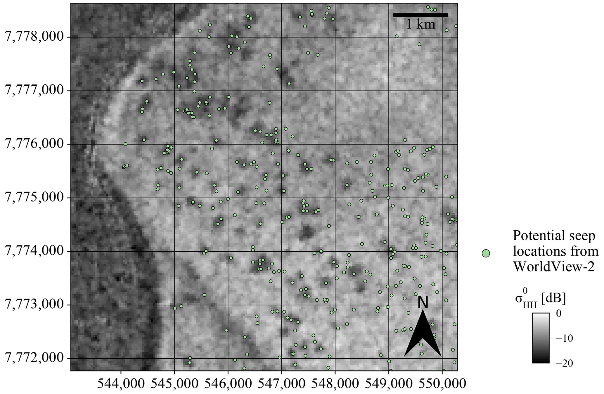
Figure 9 Comparison of detected holes (potential seep locations, green dots) from WorldView-2 imagery acquired on 22 May 2016 on top of the HH-polarisation band of a Sentinel-1 scene acquired on 7 April 2016 showing backscatter anomalies at an early stage of development. CRS: WGS 84 / UTM zone 42N.

The automated classification approach on Sentinel-1 EW data makes it possible to compose time series of areas of backscatter anomalies and compare them to time series of minimum and maximum air temperatures over the years 2015 to 2019 (Fig. 10a–e). A steady increase in area of backscatter anomalies in late winter and spring is evident. The maximum extent of backscatter anomalies was especially high in 2019, when on the last useful acquisition date, its area was approximately half of the whole lake area (Fig. 10; compare also to Fig. 4a). Maximum air temperature often approaches or slightly exceeds 0 ^∘C throughout the analysis periods. Days where maximum air temperatures exceed 0 ^∘C are shown by the dashed lines in Fig. 10. In order to assess the expansion of anomaly regions, the fraction of overlap between anomaly regions on consecutive dates is shown in brown (area of intersection between classified anomaly regions on the timestamp indicated and that of the previous timestamp, divided by area of the classified anomaly regions at the previous timestamp). The fraction is especially high during the last observation dates in the years concerned. In order to avoid division by zero, the graphs were only calculated for the time period after zero anomalies were detected for the last time in the years concerned. The fraction of overlap often increases when the air temperatures approach or exceed 0 ^∘C.

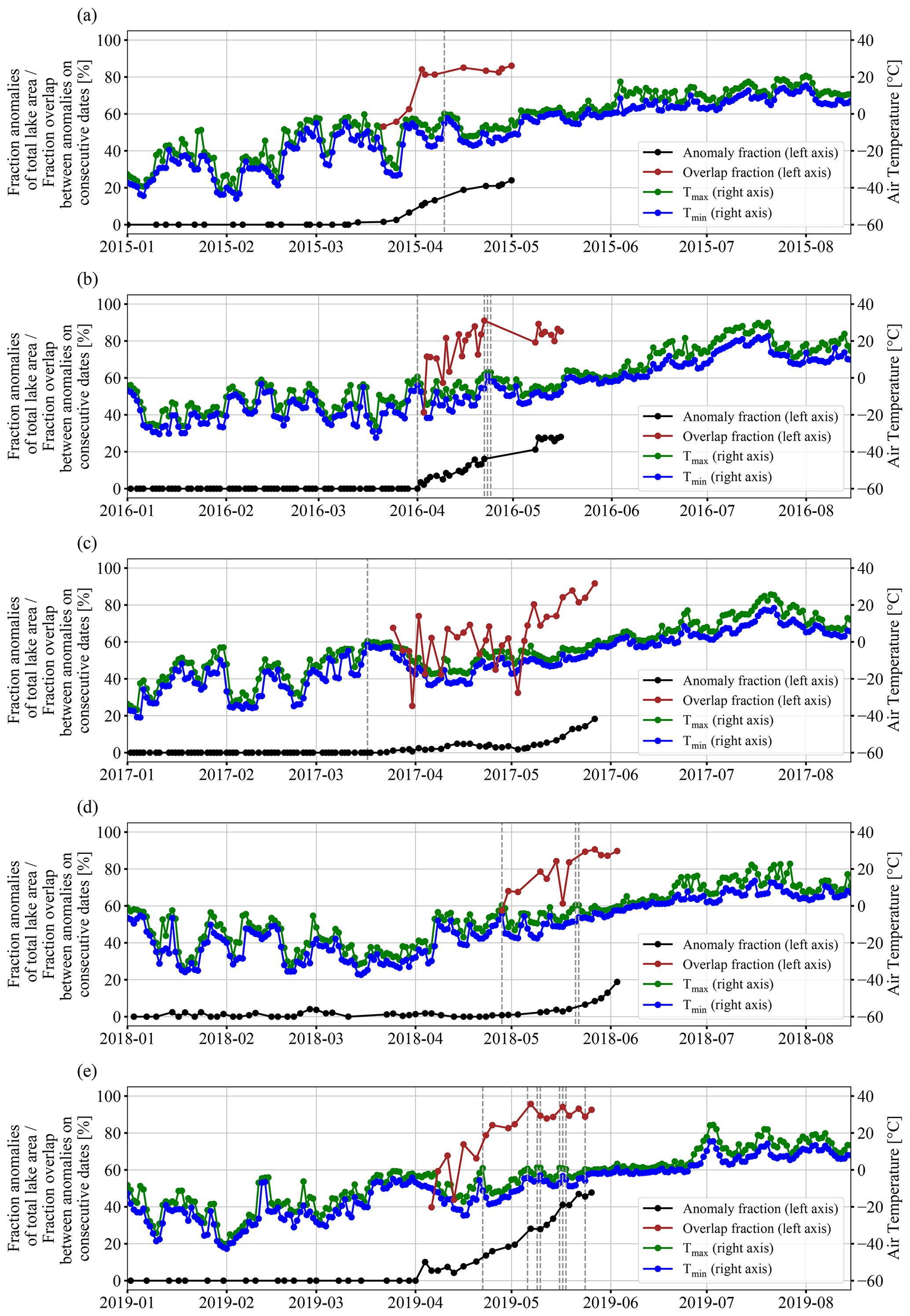
Figure 10 Time series of fraction of area of anomaly regions with respect to total lake area (black; Pointner and Bartsch, 2020), fraction of overlap between anomaly regions on consecutive dates (brown) for the time period after no anomalies were detected for the last time in the years concerned, and maximum (green) and minimum (blue) 2 m air temperature from ERA5 (Hersbach et al., 2018). The left axis indicates the fraction of area of anomaly regions with respect to total lake area and the fraction of overlap between anomaly regions on consecutive dates. The right axis indicates air temperature. Fractions of overlap were calculated as the area of intersection between classified anomaly regions on the timestamp indicated and that of the previous timestamp, divided by area of the classified anomaly regions at the previous timestamp. Dashed grey lines indicate dates where maximum air temperature exceeded 0 ^∘C during the analysis periods of the SAR data.

The results of the ALOS PALSAR-2 polarimetric analyses can be directly compared to Sentinel-1 acquisitions in EW and IW modes (Fig. 11) and to Landsat 8 brightness temperature and surface reflectance data acquired in April 2015. As expected, backscatter is clearly lower in anomaly zones than for regular floating lake ice in both Sentinel-1 IW VV-polarised (Fig. 11a) and Sentinel-1 EW HH-polarised (Fig. 11b) images. The T₁₁ component of the coherency matrix, which is related to the magnitude of surface scattering (Engram et al., 2013), interestingly indicates lower backscatter from regular floating lake ice compared to anomaly zones in the L band (Fig. 11c). The polarimetric classification (Fig. 11d) shows that regular floating lake ice largely falls in region 6 (random surface), while anomaly regions mainly fall in region 9 (Bragg surface) of the H-α plane (Lee and Pottier, 2009). The brightness temperature in anomaly regions is approximately 1 to 2 K higher than in the rest of the lake (Fig. 11e), while the snow surface appears rather homogeneous but also shows very small differences in anomaly regions in the true-colour composite of surface reflectance in Fig. 11f.

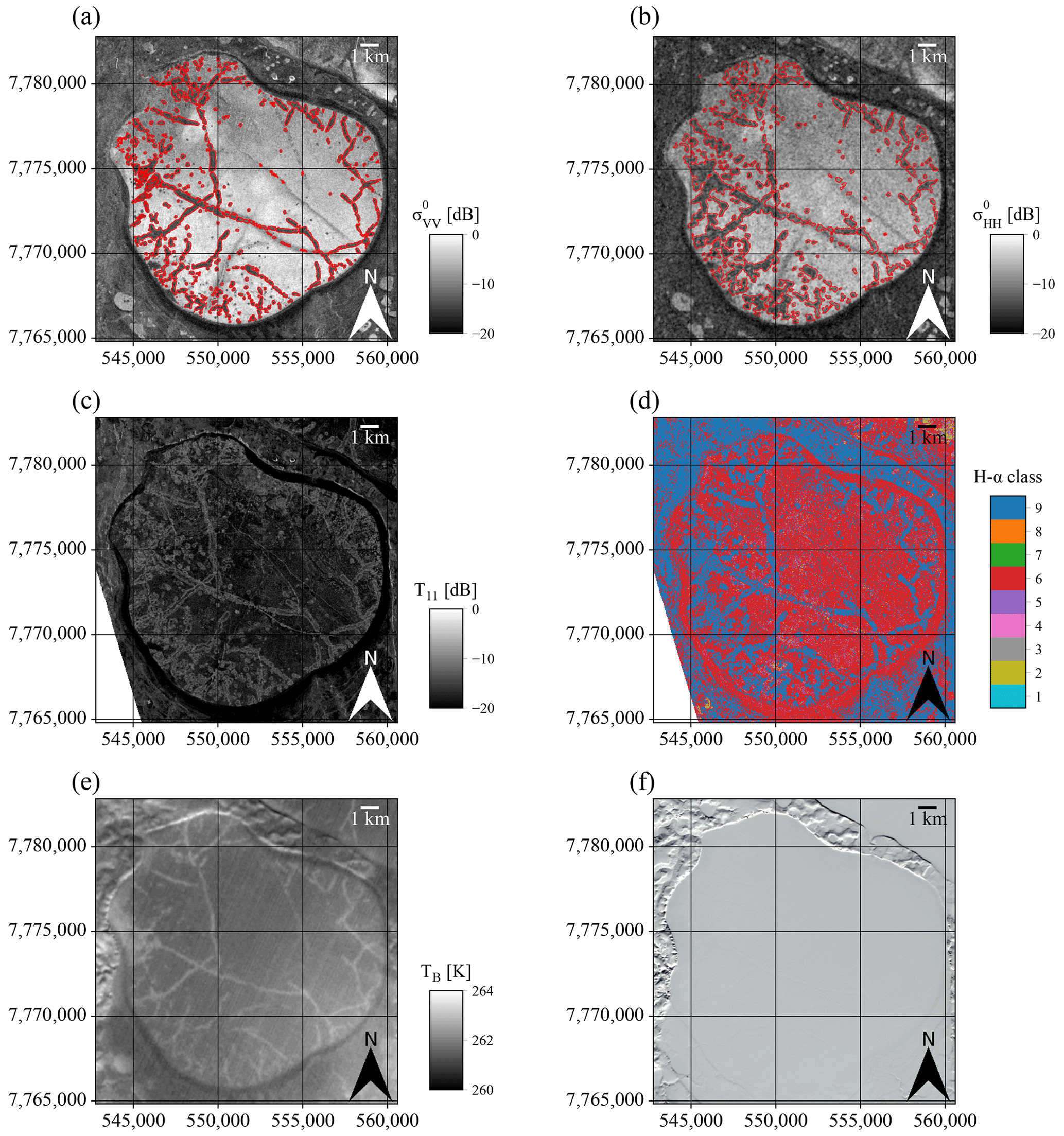
Figure 11 Comparison of Sentinel-1 C-band data, ALOS PALSAR-2 L-band polarimetric results, and Landsat 8 brightness temperature and surface reflectance for Lake Neyto in April 2015. (a) Sentinel-1 IW VV-polarised acquisition from 10 April 2015. (b) Sentinel-1 EW HH-polarised acquisition from 23 April 2015. (c) ALOS PALSAR-2 T₁₁ from 18 April 2015. (d) Polarimetric classification result from ALOS PALSAR-2 scene acquired on 18 April 2015 (pixel values denote zones in the H-α plane; zone 6 is termed “random surface” and zone 9 is termed “Bragg surface” in Lee and Pottier, 2009). (e) Landsat 8 band-10 brightness temperature from 6 April 2015. (f) Landsat 8 true-colour composite of surface reflectance data from 6 April 2015. Outlines of classified backscatter anomalies are shown in red in (a) and (b). CRS: WGS 84 / UTM zone 42N.

6 Discussion

Validation metrics from the comparison between classification results from EW and IW modes are relatively high, with similar values for the F1-score binary (0.80), the Matthews correlation coefficient (0.78) and Cohen's κ (0.78). The F1-score macro (average of F1 scores for the positive and negative class) is higher than the F1-score binary because of a significantly higher F1 score for the negative class, for which pixel occurrences are also significantly higher (compare to Sect. 4.3). Cohen's κ is especially used to measure inter-rater reliability. In the interpretation scheme proposed by Landis and Koch (1977), κ from our validation belongs to the category “substantial agreement”. A drawback is that we cannot present a proper validation against ground truth data, as often anticipated in remote sensing studies, but the remoteness of the study area and the potential endangering of human safety largely restricts in situ data collection on-site (see also Sect. 4.3).

Our results show a strong contrast between backscatter from anomaly regions and regular floating lake ice, with a difference of 5.9 dB on average across polarisation channels (Fig. 5). A striking spatial relationship between detected holes and backscatter anomaly regions is shown in Fig. 8. More than two-thirds of detected holes (potential seep locations) mapped from the WorldView-2 acquisition were found to lie within the backscatter anomaly polygons deduced from a Sentinel-1 EW acquisition taken 6 d earlier. Especially in the northern and western part of the lake, most holes can be clearly associated with the polygons deduced from the classification of the Sentinel-1 data.

A successive expansion of anomaly regions during spring is indicated by fractions of overlap between anomaly regions on consecutive dates (brown line in Fig. 10). During spring, the percentage of lake area covered by regions of anomalously low backscatter increases significantly, while the percentage of intersections remains rather high (mostly above 80 %). When comparing Fig. 9 (Sentinel-1 EW acquisition from 7 April 2016) and Fig. 8 (Sentinel-1 EW acquisition from 22 May 2016), backscatter anomalies seem to emerge from locations of detected holes in the earlier acquisition, leading to a large patch of anomalously low backscatter in the later acquisition.

There might be a connection between the expansion of anomaly regions and air temperatures, as maximum air temperatures approaching or exceeding 0 ^∘C sometimes coincide with increases in the area of anomalies (Fig. 10) and with increases in fractions of overlap between anomaly regions on consecutive dates. The shape and locations of backscatter anomaly regions vary significantly between different years (Bogoyavlensky et al., 2018; Pointner and Bartsch, 2020) (compare also to Figs. 1, 4 and 11), but the characteristic expansion is similar in all years analysed, as discussed above.

The expanding areas of anomalies in spring might therefore be related to lake ice subsidence due to significant snow load on the lake ice (April is usually considered the month of maximum snow depth and ice thickness in central Yamal) and consequent flooding through the holes over the ice top leading to wetting and/or slushing of the snowpack (see also Anonymous, 2020). The low backscatter might be consequently caused by increased absorption or specular reflection of the slush and/or wet snow. The expansion might then be caused by increasing snow loading during spring and possibly by accumulations of slush and/or wet snow around the holes. This might also be related to the increase in fractions of overlap between anomaly regions on consecutive dates when air temperature is close to or above 0 ^∘C. Patterns identified in the WorldView-2 image from 22 May 2016 that might potentially depict accumulations of slush and wet snow around the holes are shown in Fig. 12a–d, but in situ data are needed to test this hypothesis.

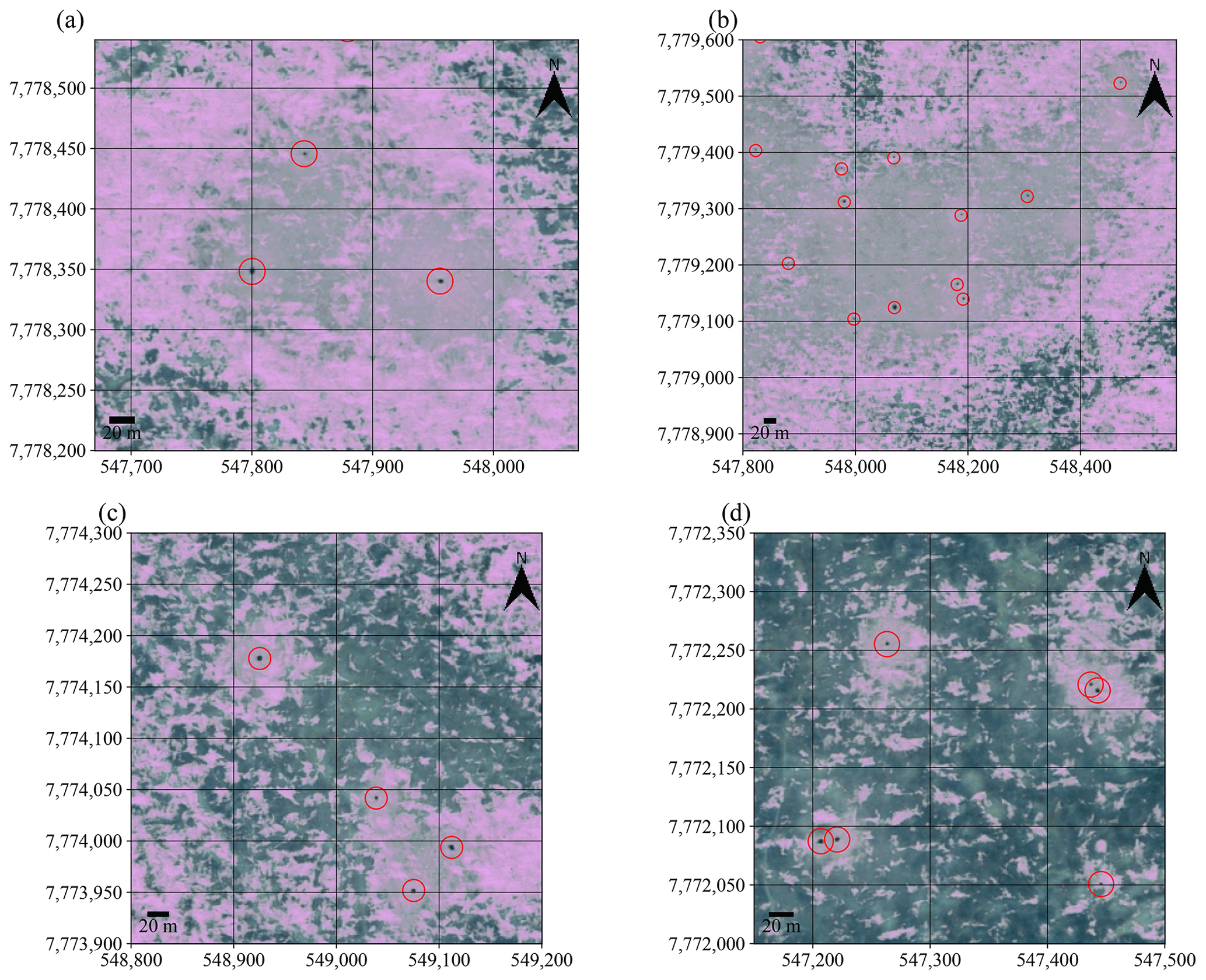
Figure 12 Examples of patterns around holes in a true-colour composite of the WorldView-2 image acquired on 22 May 2016. Red circles indicate locations of detected holes as identified by the blob-detection algorithm. CRS: WGS 84 / UTM zone 42N.

During lake ice drilling in Yamal in April 2019, the water level on several lakes rose up to 40 cm higher than the level of lake ice (Fig. 13). This could be a similar effect to the one that might be responsible for the observed anomalies on Lake Neyto, but in situ data collected on the ice of Lake Neyto would be required to verify this.

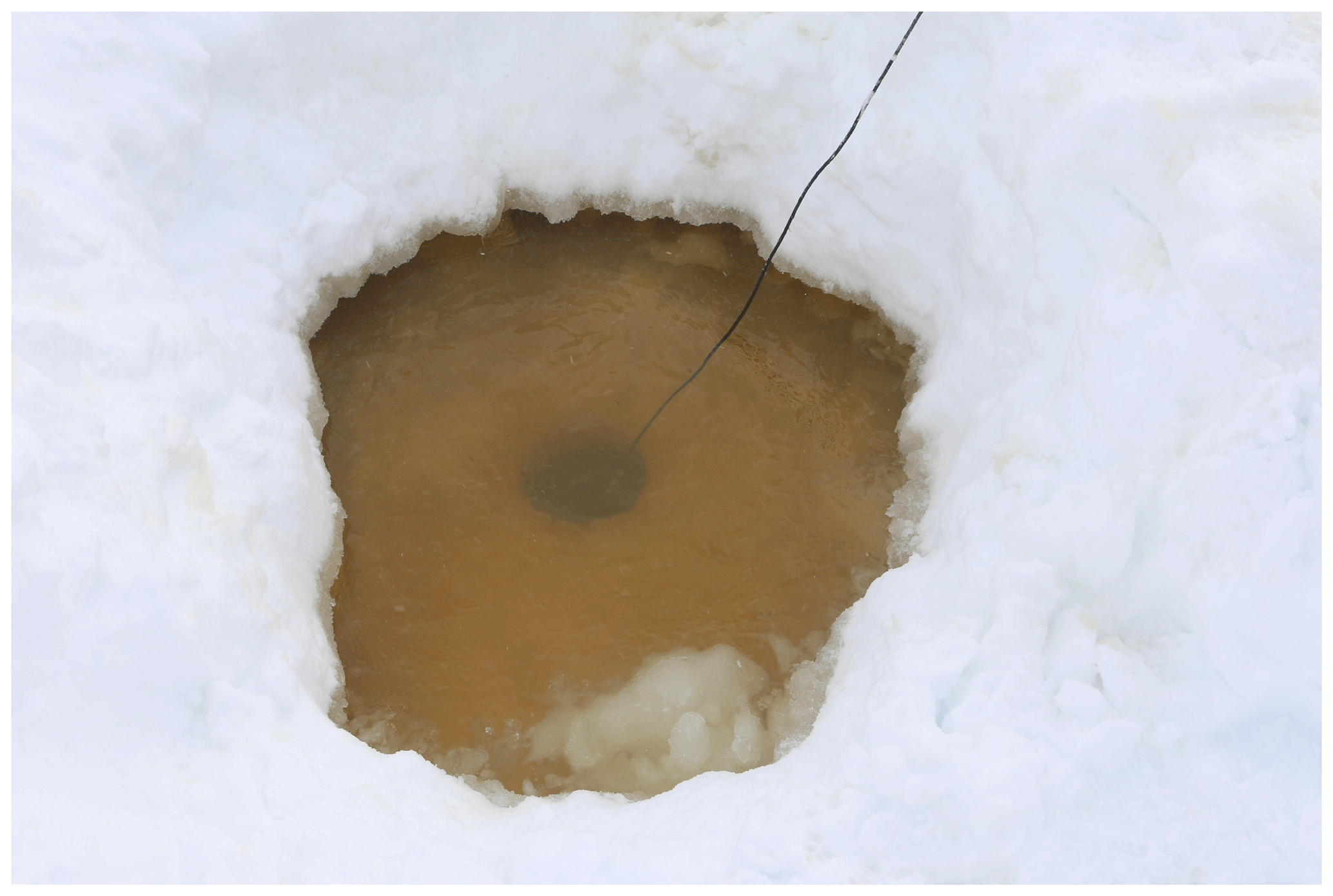
Figure 13 Liquid water on ice during lake ice drilling in central Yamal, April 2019. The lake in the photo is termed LK-013, observed and drilled on 6 April 2019 (ca. 14:00 local time). The coordinates (WGS 84 geographic) are 70.262123^∘ N, 68.884803^∘ E. Ice thickness at the time of drilling was approximately 1.5 m.

Some potentially interconnected factors might possibly explain why 29 % of detected holes are located outside the classified anomaly regions. It is noticeable that the distances between many detected holes and the anomaly region polygons is relatively short (median 67 m). The snow around these holes might have flooded after the time of the Sentinel-1 acquisition, and/or the limited spatial resolution might also play a role. Other potential reasons for holes outside classified anomaly regions may include remaining speckle, the imperfectness of the classification method in general or variations in snow depth leading to less flooding around some holes, but other unknown reasons might also contribute.

Features in the outcomes of polarimetric analyses on the L-band PALSAR-2 data from April 2015 clearly resemble backscatter anomaly regions in C-band Sentinel-1 imagery (Fig. 11a–d) as do features in the Landsat 8 brightness temperature image (Fig. 11e). We could also identify very small differences in surface reflectance in the anomaly zones (Fig. 11f), but since the whole lake appears to be covered with snow, the most obvious interpretation for the differences in brightness temperature seems to be that there is some warming from beneath the snow surface, leading to slightly increased snow surface temperatures in anomaly regions but not to full melting of the snow. This might also explain why snow seems to have melted earlier in anomaly regions in the Sentinel-2 acquisition from 21 May 2016 in Fig. 1a, but as no data on emissivity of the surface were available, we cannot reach a conclusion on actual snow surface temperatures, and the limited spatial resolution of Sentinel-2 and Landsat 8 could prevent the identification of smaller details on the ice or snow surfaces.

While T₁₁ values are similar between many centres of anomaly regions and regular floating lake ice, high values of T₁₁ are observed mainly from the outlines of anomaly regions (Fig. 11c), which might potentially relate to different scattering mechanisms for slush and wet snow, but further data are required to assess this and understand scattering mechanisms at both C-band and L-band frequencies. An explanation for the classification of anomaly regions in the L band as Bragg surface (zone 9 in Cloude and Pottier, 1997) in Fig. 11d also calls for further investigations.

The observation that C-band backscatter is relatively high and L-band T₁₁ is relatively low in the case of regular floating lake ice may be explained by the longer radar wavelength in the L band. Recent studies suggest that backscatter from regular floating lake ice is predominantly caused by surface scattering controlled by roughness from the ice–water interface for both C-band (Atwood et al., 2015; Gunn et al., 2018) and L-band (Atwood et al., 2015; Engram et al., 2020, 2013) SAR. Our polarimetric classification result (Fig. 11d) clearly supports these findings, as it indicates that the main scattering mechanism from regular floating lake ice of Lake Neyto is scattering from a random surface (zone 6 in Cloude and Pottier, 1997) at the L band. Whether a surface can be considered rough, which is related to the magnitude of backscatter, largely depends on the magnitude of local height variations in relation to the radar wavelength (e.g. Woodhouse, 2005). The local height variations of the ice–water interface of regular floating lake ice of Lake Neyto may be too small for the surface to be considered rough at the L band (approximately 23 cm wavelength) but large enough to be considered rough at the C band (approximately 5.5 cm wavelength).

Engram et al. (2020) show that L-band T₁₁ (ALOS PALSAR-1) is positively correlated with the area of methane bubbles trapped in lake ice and also with total lake methane flux estimates for thermokarst lakes in Alaska. However, there are some significant differences between the studies of Engram et al. (2020) and this study that should be pointed out. Engram et al. (2020) primarily use autumn acquisitions, although correlations with spring L-band backscatter were also shown in Engram et al. (2013). The increased radar return from ebullition zones is attributed to surface scattering from cavities that form due to slower ice growth above discrete point-like ebullition sources, which tend to remain in the same location every year (Engram et al., 2020). As a consequence of slowed ice growth, the cavities are filled by water, partly filled by gas or completely filled by gas (Engram et al., 2020). Resulting rough surfaces are the ice–water interface or the gas–water interface (Engram et al., 2020). Bogoyavlensky et al. (2018) and Pointner and Bartsch (2020) showed that locations of backscatter anomalies vary significantly between years for Lake Neyto. Cavities related to ebullition responsible for increased L-band T₁₁ in PALSAR-1 SAR imagery in Engram et al. (2020) are of a much smaller spatial scale than the holes in the VHR imagery of Lake Neyto. Diameters of reported cavities in Engram et al. (2020) are on the order of decimetres, while the median area of 718 open holes identified in this study is 4 m². Engram et al. (2020) note that hotspot-type seeps are the rarest in Alaskan lakes and ebullition fluxes are dominated by much weaker A-type (characterised by isolated bubbles in multiple ice layers) and B-type (characterised by merged bubbles in multiple ice layers) seeps in the seep classification scheme of Walter Anthony et al. (2010).

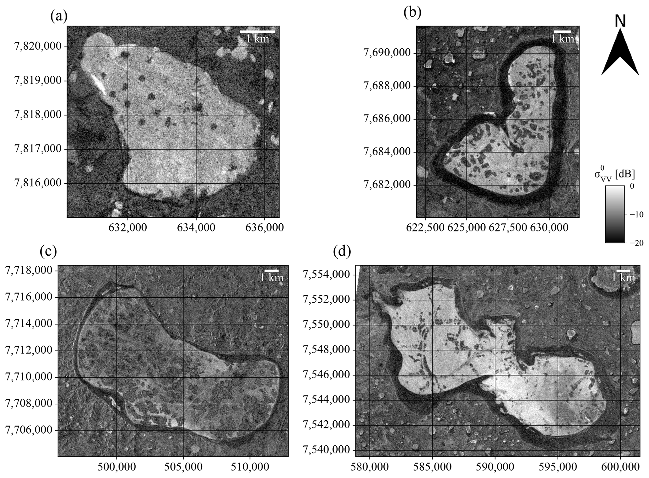
Figure 14 Examples of Sentinel-1 IW mode VV-polarised images of other lakes in Yamal with regions of anomalously low backscatter similar to those on Lake Neyto. (a) Lake Yanunto on 25 May 2019. (b) Lake Penadoto on 25 May 2017. (c) Lake Yambuto on 16 May 2018. (d) Lake Yarroto-2 on 3 May 2019. CRS: WGS 84 / UTM zone 42N.

Hotspots of gas emissions have previously been described to be visible as black holes (compare to Figs. 1 and 6) in lake ice (Walter, 2006; Walter et al., 2006), and the size (Fig. 7) and spatial clustering (Figs. 8 and 9) of holes identified in this study seem consistent with observations of holes related to subcap seepage in Walter Anthony et al. (2012). However, other causes of holes in lake ice were identified for Lake Baikal, for example, such as seal breathing holes, hot springs or oil seepage (Galaziy, 1987; Petrov, 2009). Ebullition of geologic methane as the cause of the holes in the ice of Lake Neyto would be consistent with studies by Bogoyavlensky et al. (2019a, 2018, 2016) and Kazantsev et al. (2020), but in situ measurements are needed to confirm this hypothesis.

The gas that might be associated with the observed backscatter anomalies was previously suggested to be originated from the gas field that stretches out under Lake Neyto and/or from the dissociation of gas hydrates within the permafrost (Bogoyavlensky et al., 2018). In April 2019, the wheel of an all-terrain vehicle fell into a patch of very thin ice on one of the lakes in central Yamal, 60–70 km from Lake Neyto. Later in August, two gas seeps were found in this particular place. The emissions of pure methane of biogenic origin from these two seeps were estimated as more than 100 kg yr⁻¹ (Kazantsev et al., 2020). The isotopic composition of collected methane and the size of the lake suggest that the gas has been delivered from permafrost and not from the deep productive horizons (Dvornikov et al., 2019). The potential annual amount of methane emitted from only two small seeps described in Kazantsev et al. (2020) is comparable with the annual diffuse emission from the entire lake area of West Siberian lakes (5–249 kg yr⁻¹; Kazantsev et al., 2018) given that it is completely covered with ice throughout 6 to 7 months of the year. Therefore, the emission of seepage methane may continue throughout the whole year.

It should be noted that similar patches of anomalously low backscatter in Sentinel-1 SAR imagery have also been shown for a number of lakes in the vicinity of Lake Neyto by Bogoyavlensky et al. (2018) and for Lake Yambuto (approximately 70 km southwest of Lake Neyto) by Pointner et al. (2019). Further, more than 300 lakes near Seyakha in Yamal that may show traces of gas emissions as either craters at the bottom or holes in lake ice were identified in optical VHR satellite imagery by Bogoyavlensky et al. (2019a).

Here, we have shown the potential connection between open holes in lake ice potentially caused by gas emissions and patches of anomalously low backscatter in C-band SAR imagery for the first time, but in situ data are needed to understand the phenomenon in detail. Upon the verification of the presented hypothesis, the capability of SAR instruments to collect useful data under almost all weather conditions, high revisit rates and high coverage may allow the identification of other lakes with subcap gas emissions from C-band SAR data in future studies at larger spatial extents. This might then aid our understanding of how much methane is released from West Siberian lake seeps and might possibly contribute to an incorporation of emissions from these seeps in climate models.

Figure 14a–d show examples of lakes in Yamal (including Lake Yambuto) with similar regions of low C-band backscatter (Fig. 14a–d). Because of a higher spatial resolution, images acquired by Sentinel-1 in IW mode and VV polarisation are shown. While Sentinel-1 IW data can depict anomalies in greater spatial detail, they are unfortunately acquired at lower temporal frequencies and more irregularly in comparison to the EW data over Yamal (see also Sect. 3.1). Anomalies on these lakes appear similar to those on Lake Neyto, but whether they (including those on Lake Neyto) are indeed related to methane ebullition has yet to be verified. Based on the spatial and temporal dynamics of the C-band backscatter anomalies on Lake Neyto, a method that incorporates both spatial and temporal information of C-band SAR data could be favourable for identifying anomalies over larger spatial extents.

7 Conclusions

In this study, we investigated and quantified anomalies of C-band radar backscatter in SAR images of lake ice of Lake Neyto in Yamal, Russia, and assessed their potential relation to gas emissions. This relation was suggested before using visual comparisons between Sentinel-1 data and medium-resolution optical data, but here we provided a quantification of relations between features in SAR and VHR imagery, examined the spatio-temporal dynamics of backscatter anomaly regions, and assessed potential scattering and formation mechanisms in greater detail. The spatial relationship between 718 holes detected from WorldView-2 imagery and anomalies mapped from Sentinel-1 EW imagery acquired a few days apart and more than a month earlier suggests that anomalies expand from the locations of many holes. Expanding anomalies might be caused by flooding of the ice and subsequent slushing and/or wetting of the snow around the holes, as the ice surface around the holes might be depressed below the hydrostatic water level due to increased snow loading in spring. This explanation is inferred from observed flooding of the ice layer during ice drilling on another lake in central Yamal in spring, but in situ observations of ice of Lake Neyto are needed to test this hypothesis. Statistics of areas and spatial clustering of mapped holes are consistent with observations related to subcap seepage of methane reported in previous studies, but it has yet to be verified that the holes in ice of Lake Neyto are indeed caused by up-welling gas. The proposed method to automatically map backscatter anomalies delivered good results in relation to the chosen validation strategy and could potentially also allow for monitoring of gas emissions on Lake Neyto in the future upon the verification of this hypothesis. The spatial and temporal properties of Sentinel-1 SAR data may also allow for the identification of lakes with similar anomalies to those of Lake Neyto over larger spatial extents in the near future, and, if the given hypothesis is correct, this might potentially aid our understanding of how much methane is released by West Siberian lake seeps.