the Creative Commons Attribution 4.0 License.
the Creative Commons Attribution 4.0 License.
 | 26 Mar 2021
Improved machine-learning-based open-water–sea-ice–cloud discrimination over wintertime Antarctic sea ice using MODIS thermal-infrared imagery
Marcus Huntemann
The frequent presence of cloud cover in polar regions limits the use of the Moderate Resolution Imaging Spectroradiometer (MODIS) and similar instruments for the investigation and monitoring of sea-ice polynyas compared to passive-microwave-based sensors. The very low thermal contrast between present clouds and the sea-ice surface in combination with the lack of available visible and near-infrared channels during polar nighttime results in deficiencies in the MODIS cloud mask and dependent MODIS data products. This leads to frequent misclassifications of (i) present clouds as sea ice or open water (false negative) and (ii) open-water and/or thin-ice areas as clouds (false positive), which results in an underestimation of actual polynya area and subsequently derived information. Here, we present a novel machine-learning-based approach using a deep neural network that is able to reliably discriminate between clouds, sea-ice, and open-water and/or thin-ice areas in a given swath solely from thermal-infrared MODIS channels and derived additional information. Compared to the reference MODIS sea-ice product for the year 2017, our data result in an overall increase of 20 % in annual swath-based coverage for the Brunt Ice Shelf polynya, attributed to an improved cloud-cover discrimination and the reduction of false-positive classifications. At the same time, the mean annual polynya area decreases by 44 % through the reduction of false-negative classifications of warm clouds as thin ice. Additionally, higher spatial coverage results in an overall better subdaily representation of thin-ice conditions that cannot be reconstructed with current state-of-the-art cloud-cover compensation methods.
- Article
(9144 KB) - Full-text XML
- BibTeX
- EndNote


Information on cloud presence is of crucial importance when using thermal-infrared imagery. This is especially true for the polar regions, where the thermal contrast between clouds and the underlying snow and sea-ice surface can be low through persistent surface temperature inversion and low clouds (Welch et al., 1992). Furthermore, occurrences of warm clouds over cold sea ice and cold clouds over relatively warm and thin sea ice are both possible. Despite improvements (Liu et al., 2004; Frey et al., 2008; Holz et al., 2008; Liu and Key, 2014), the performance of the frequently used Moderate Resolution Imaging Spectroradiometer (MODIS) cloud mask product (MOD35/MYD35; Ackerman et al., 2015) is substantially reduced during polar nighttime compared to its performance during daytime conditions.
Nonetheless, several studies use MODIS thermal-infrared (TIR) data to monitor polynya area and associated sea-ice production in polynyas both in the Arctic as well as the Antarctic and compare well to or even outperform studies using passive-microwave satellite data in certain regions (e.g., Paul et al., 2015; Aulicino et al., 2018; Preußer et al., 2019). These studies generally utilize ice-surface temperature from the National Snow and Ice Data Center (NSIDC) sea-ice product (MOD/MYD29; Hall et al., 2004; Hall and Riggs, 2015a, b). The MOD/MYD29 product is derived from both MODIS sensors on board the NASA polar-orbiting Aqua and Terra satellites with the MOD/MYD35 cloud mask product already applied (Riggs and Hall, 2015). However, especially positive temperature-anomaly features such as large warm open-water areas through sea-ice polynyas pose a problem for the MODIS cloud mask and result in frequent misclassification of these areas as cloud cover (Fraser et al., 2009). Additionally, other MODIS applications would potentially benefit from an improved wintertime cloud masking. These applications comprise composite generation (e.g., Fraser et al., 2010, 2020), merged optical and passive microwave sensor applications (e.g., Ludwig et al., 2019), basin-wide lead detection from thermal-infrared data (e.g., Reiser et al., 2020), and sea-ice motion tracking through image cross-correlation.

Figure 1Location of the general (orange) and focus (purple) study area of the Antarctic Brunt Ice Shelf in the southeastern Weddell Sea (green). Data of land ice (dark gray) and floating ice shelves (light gray) are retrieved from RTopo-2 (Refined Topography; Schaffer et al., 2016).
In this study, we propose a novel machine-learning-based approach to discriminate between open-water and/or thin-ice, sea-ice, and cloud-covered areas in MODIS TIR swaths. We evaluate and analyze the use of a deep neural network (e.g., Kohonen, 1988; Goodfellow et al., 2016), building upon a comprehensive set of newly generated labeled training data. The data set is derived using a combined approach of unsupervised deep learning, subsequent clustering, and manual screening from co-located 1 km resolution MOD/MYD02 product data (MODIS Characterization Support Team (MCST), 2017a, b) accessed through the Level-1 and Atmosphere Archive & Distribution System (LAADS) Distributed Active Archive Center (DAAC) and the Sentinel-1 A/B (S1-A/B) synthetic aperture radar (SAR) calibrated backscatter data accessed through the Alaska Satellite Facility (ASF) DAAC as a cloud-independent reference.
The resulting classifier performance is then analyzed and evaluated based on wintertime estimates of the resulting polynya area in comparison to the MOD/MYD29 reference product for the Brunt Ice Shelf (BIS) region in the Antarctic Weddell Sea in the year 2017 (Fig. 1). This region was chosen for its combination of high inter-annual polynya activity and high spatiotemporal coverage with Sentinel-1 data. Results are expected to be transferable to other polynya regions in the Antarctic.
In the following sections, we will first describe our methodology and input data starting with the employed basic methods and algorithms (Sect. 2.1) followed by the used input data (Sect. 2.2), a detailed explanation of the initial-training-data generation scheme (Sect. 2.3), and the subsequent processing steps that lead to our final classifier (Sect. 2.4 and 2.5). Finally, we describe and discuss our results (Sect. 3) in comparison to standard MOD/MYD29-derived estimates as well as using co-located S1-A/B SAR reference data. In the end we provide a summary and an outlook for future applications (Sect. 4).

Figure 2Flow chart summarizing all processing steps from the generation of the initial training data through manual classification of the swath-based split of the data into a calibration and a validation data set (Cal/Val) to the training of the final classifier and its application for open-water–sea-ice–cloud discrimination.
In the following subsections we describe our methods and input data that lead to our deep neural network for the open-water–sea-ice–cloud discrimination (Fig. 2).
2.1 Basic methods and algorithms
This section intends to provide a basic introduction to the methods used in this study. However, it would be beyond the scope of this article to provide an exhaustive review of these methods. For more details, additional references are provided.
All computations for this study were carried out using the R software (R Core Team, 2018) running on a commercially available laptop.
2.1.1 Gray-level co-occurrence matrices (GLCMs)
Gray-level co-occurrence matrices (GLCMs) are a tool to quantify spatial texture based on brightness values of a pixel neighborhood (Haralick et al., 1973; Haralick, 1979; Hall-Beyer, 2017; R: Zvoleff, 2019). The directional-dependent occurrence frequencies of brightness-value combinations are counted and normalized to probabilities. Subsequently, several statistical measures can be calculated from the GLCM as an additional descriptive statistic of the data.
Haralick et al. (1973) proposed 14 different metrics; however, not all were commonly adopted and implemented into modern software. For R, eight different measures are implemented (Zvoleff, 2019), of which we utilized four: GLCM mean, GLCM variance, contrast, and entropy (Table 1).
Hall-Beyer (2017) showed that GLCM variance can be associated with edges of different class patches, while GLCM mean and contrast and entropy correspond well to patch-interior texture.
In general, the use of GLCM texture metrics is suitable for cloud detection and classification in polar regions using visual, near-infrared, and thermal-infrared satellite data (Welch et al., 1992). However, as the size of each GLCM per pixel in a sliding-neighborhood window corresponds and increases proportionally to the image bit depth, computational cost increases rapidly for (i) large sliding windows and (ii) a large number of gray levels in the input data. For our study, all MOD/MYD02 channel-based input parameters for the GLCM computations were rescaled to 32 gray levels, using a 7 × 7 sliding-neighborhood window with horizontal, vertical, and diagonal directional pixel relationships.
2.1.2 Fuzzy c-means clustering (FCM)
For clustering of our initial training data, we utilize an unsupervised procedure called fuzzy c-means clustering (FCM; Dunn, 1973; Bezdek et al., 1984; R: Meyer et al., 2019).
The FCM is comparable to a classic k-means clustering approach (MacQueen, 1967; Hartigan and Wong, 1979), with the addition of providing cluster membership probabilities for each pixel. This type of clustering is also referred to as “soft” clustering. In contrast to “hard”-clustering approaches such as k-means, FCM allows for a pixel to belong to several clusters with a certain probability.
For this type of unsupervised clustering, it is necessary to preselect the number of clusters which the input data should be separated into. Without a priori knowledge about potential relationships and correlations between predictors, it is common practice to choose a large number of initial clusters and manually merge similar clusters afterwards to the desired number of classes.
In this study, we always use a setup of 35 clusters and stop the clustering process after 30 iterations.
2.1.3 Artificial neural networks (NNs)
An artificial neural network (NN) generally consists of several neurons organized in sequential layers in which each neuron of a layer is fully interconnected to all neurons in the adjacent two layers through weighted paths. These neurons respond to the weighted input of the preceding neurons and pass on their output to the adjacent neurons, modulated based on a type of activation function (Kohonen, 1988; Lee et al., 1990; Welch et al., 1992; Atkinson and Tatnall, 1997; LeCun et al., 2015; Schmidhuber, 2015; Goodfellow et al., 2016; R: Allaire and Chollet, 2020).
Once trained, NNs are powerful tools for fast and efficient processing of large amounts of remote sensing data and have been shown to be more accurate, e.g., in classification tasks, than other techniques (Kohonen, 1988; Lee et al., 1990; Atkinson and Tatnall, 1997).
Furthermore, NNs can represent complex and non-linear functions without formal description through learning from labeled training data. In contrast to statistical methods, NNs allow for incorporating data from different sources and require no knowledge or assumptions about their parametric distributions. Hence, NNs solely depend on their provided input data (Lee et al., 1990; Atkinson and Tatnall, 1997; LeCun et al., 2015).
In their simplest form, a so-called “shallow” NN consists of an input layer, a hidden layer, and an output layer. Input-layer neurons correspond to the number of input features or predictors, whereas output layer neurons correspond in the case of classification tasks to the number of classes the input data should be categorized into. With an increasing number of hidden layers, so-called “deep” NNs can handle even more complex problems (Atkinson and Tatnall, 1997; Schmidhuber, 2015).
While some general suggestions for the NN architecture exist, solutions are often found empirically by minimizing or maximizing the loss function or accuracy for both calibration and validation data classification without overfitting the model. This process is described in the following subsections.
In addition to these general NNs, we work with a second type called an autoencoder (AE). An AE is a specialized variant of an NN used for anomaly detection and dimension reduction (Cao et al., 2018; Dong et al., 2018; R: Allaire and Chollet, 2020).
In a typical AE, the output or target data are equal to the input data. However, all information is forced through a bottleneck hidden layer. The result relies on the capability of the bottleneck hidden-layer neurons to extract relevant information from the training data to enable the AE to reconstruct the input image with minimized error (Cao et al., 2018).
This is achieved by constructing two branches of symmetric hidden layers of neurons (called the encoder and the decoder, respectively) around a bottleneck neuron layer generally consisting of very few neurons (Cao et al., 2018). The resulting encoder part of the AE can then be used for dimension reduction.
Table 1Summary of all used parameters, their source product or sensor, and their application in this study. These parameters comprise the brightness temperature (BT) from the selected MOD/MYD02 channel subseta as well as normalized BT (BTnormb). Furthermore, ice-surface temperatures (IST) from MOD/MYD02 are presented together with the IST from neighboring swaths (ISTNeighbors) and the time-normalized IST change (ISTΔt) between them as well as the IST from the MOD/MYD29 product. The texture metrics calculated from GLCM (mean, variance, contrast, and entropy) as well as the calibrated backscatter (σ0) from Sentinel-1 A/B are given as a reference (R). Finally, the atmospheric parameters taken from the ERA-Interim reanalysis necessary for the calculation of thin-ice thickness (TIT) are presented. The applications comprise primarily their use in the training of the neural network (NN) and autoencoder (AE).
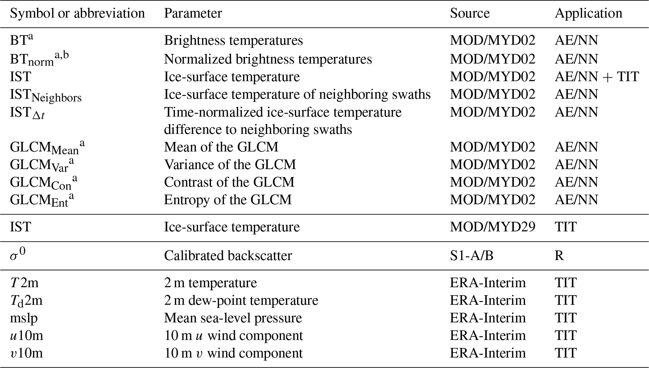
AE/NN: autoencoder or neural network; R: reference; TIT: thin-ice thickness calculation. a Calculated or derived for MODIS channels 20, 25, 31, and 33; b normalized through swath-wide mean and standard deviation: BT.
2.2 Input data
In total, we use four different types of data sets for the year 2017:
-
MODIS Level 1B calibrated radiances obtained from the MODIS sensors on board the polar-orbiting NASA satellites Terra and Aqua (MOD/MYD02; MODIS Characterization Support Team (MCST), 2017a, b; retrieved from the LAADS DAAC at https://ladsweb.modaps.eosdis.nasa.gov/, last access: 7 August 2019) with a spatial resolution of 1 km × 1 km at nadir and swath dimensions of 1354 km (across track) × 2030 km (along track),
-
Sentinel-1 A/B Level 1 calibrated backscatter data (S1-A/B; retrieved from the ASF DAAC at https://asf.alaska.edu/, last access: 25 June 2019, and processed by ESA) with a spatial resolution of 20 m × 20 m,
-
NSIDC MODIS sea-ice product (MOD/MYD29; Hall et al., 2004; Riggs and Hall, 2015) in the same resolution as the MOD/MYD02 data but comprising a precomputed and MODIS cloud-mask-applied ice-surface temperature (IST) data set, and
-
ECMWF ERA-Interim atmospheric reanalysis data (Dee et al., 2011) featuring a spatial resolution of 0.75∘ and a temporal resolution of 6 h.
An overview of all used input parameters with their respective source as well as their application is provided in Table 1.
All MODIS and ERA-Interim data are resampled to a common equirectangular grid of the Brunt Ice Shelf (BIS) area with an average spatial resolution of 1 km × 1 km and an extent from 34 to 18∘ W and 77 to 73∘ S using a nearest-neighbor approach. For visual reference, the S1-A/B data are also resampled to an equirectangular grid with the same extent but a spatial resolution of 25 m. Through the decreasing distance between meridians towards the pole, the per-pixel spatial area also decreases. This results from the constant latitudinal distance between grid points in this type of projection. Ice-shelf areas are excluded from our analysis based on RTopo-2 data (Schaffer et al., 2016).
2.2.1 MOD/MYD02 L1b calibrated radiances
Our goal for the later discrimination algorithm was for it to solely rely on MODIS-channel data, without the need for any auxiliary data.
Brightness temperatures (BTs) were calculated from calibrated radiances comprising MODIS channels 20, 25, 31, and 33 following Toller et al. (2009). This channel subset allows for distinguishing between open-water and/or thin-ice, sea-ice, and cloud pixels through a high inter-channel variability while reducing the impact of stripes in the MODIS data. Additionally, channel 32 data are used for the calculation of the ice-surface temperature (IST; following Riggs and Hall, 2015). Furthermore, we computed image-texture parameters using GLCM (Table 1). For this we use MODIS Collection 6.1 data.
We generally limited our study to swaths featuring sensor incidence angles of ≤ 50∘ in 65 % of the study area (to minimize spatial distortion towards the swath edges) and a total coverage of our study area of > 90 %. In order to aid the manual categorization by providing favorable geometries, the MODIS colocation swath to the S1-A/B reference data needs to feature sensor incidence angles of ≤ 35∘ in 65 % of the study area.
2.2.2 MOD/MYD29 sea-ice product
For a later comparison based on cloud coverage and polynya area, we extracted and use IST from the reference NSIDC MOD/MYD29 sea-ice product produced from MODIS Collection 6 data, which offers an overall accuracy of 1–3 K under ideal (i.e., clear-sky) conditions (Hall et al., 2004; Riggs and Hall, 2015).
Both IST values (MOD/MYD02 and MOD/MYD29) are derived based on a constant emissivity for snow or ice (Hall et al., 2015) but with the MODIS cloud mask already applied to the MOD/MYD29 product.
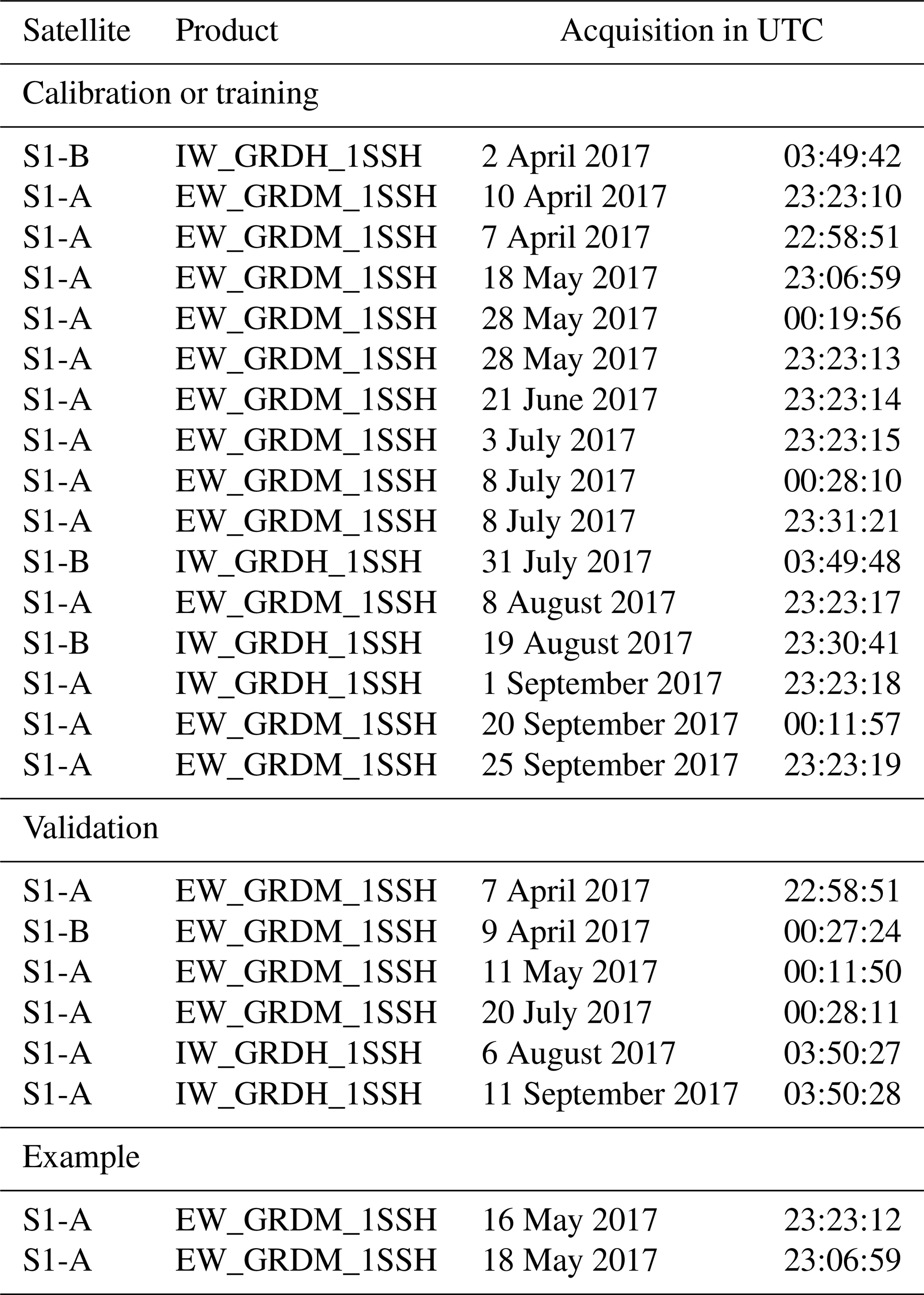
Table 2List of used S1-A/B swaths for calibration or training, validation, and a detailed analysis (Fig. 6).
2.2.3 S1-A/B L1 calibrated backscatter
In order to reliably identify polynyas independent of cloud cover or other atmospheric disturbances, we selected a total of 22 S1-A/B swaths featuring an active polynya in front of the BIS.
These S1-A/B swaths together with co-located and at least partially cloud-free MOD/MYD02 data are used for calibration and validation of the algorithm. S1-A/B swath acquisition times are temporarily distributed over the 2017 Antarctic winter, with all additional information summarized in Table 2.
2.2.4 ERA-Interim data and thin-ice retrieval
For a quantitative comparison between the resulting polynya area (i.e., the total area of pixels covered with a maximum ice thickness of 0.2 m), we calculate the thin-ice thickness (TIT) from MODIS IST for MOD/MYD02 and MOD/MYD29 data using a surface-energy-balance model together with the ERA-Interim 2 m air temperature, the 10 m wind-speed components, the mean sea-level pressure, and the 2 m dew-point temperature (Dee et al., 2011).
The surface-energy-balance model utilizes the inversely proportional relation between IST and the thickness of thin sea ice (Yu and Rothrock, 1996; Drucker et al., 2003). The net positive flux towards the atmosphere between the warm ocean and the cold atmosphere is equalized from the conductive heat flux through the ice. From the conductive heat flux TIT is derived. A detailed description of the retrieval procedure and all equations and necessary assumptions are thoroughly described in Paul et al. (2015) as well as Adams et al. (2013). For ice thicknesses between 0.0 and 0.2 m, Adams et al. (2013) state an average uncertainty of ±4.7 cm.
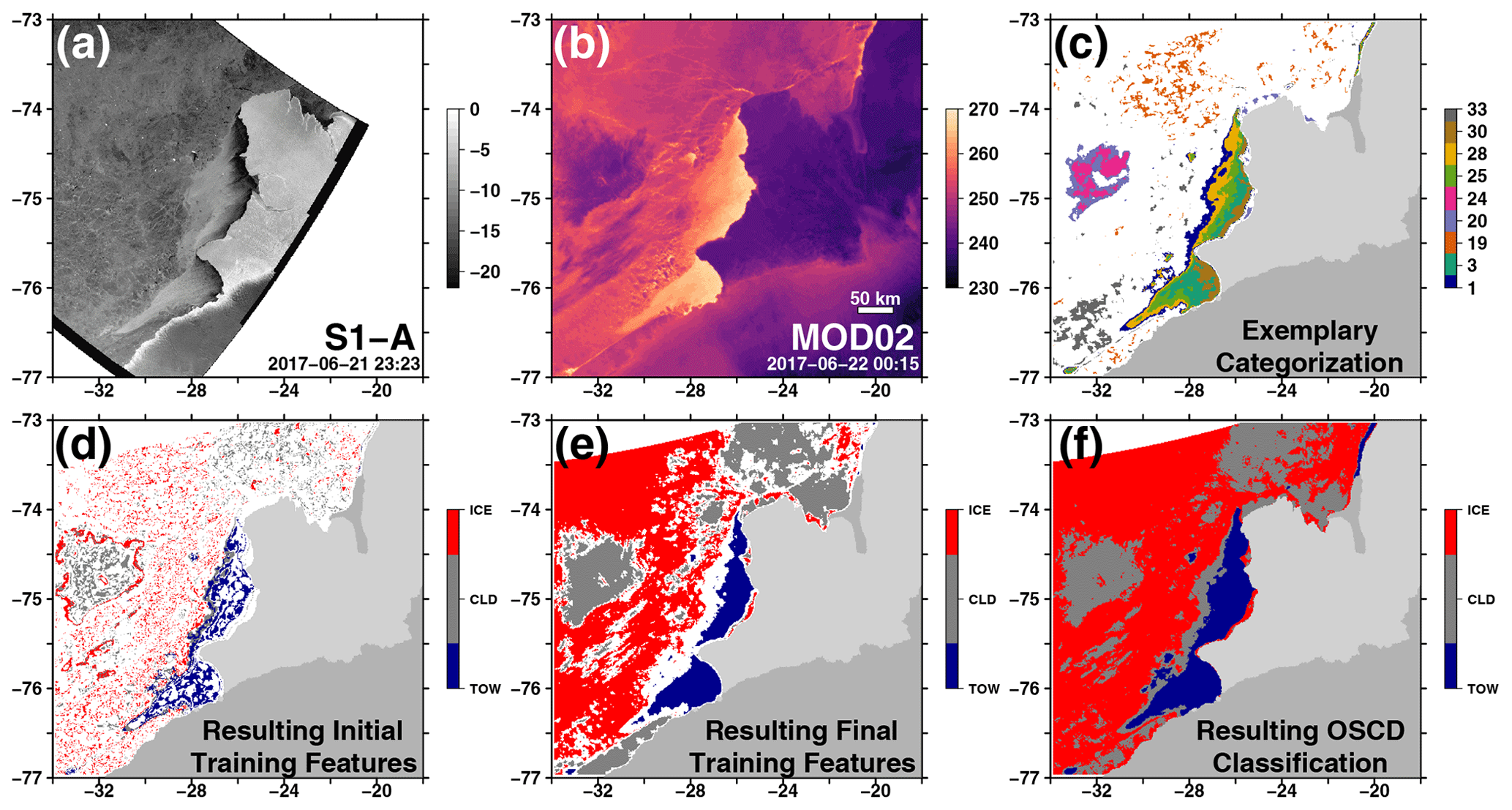
Figure 3Exemplary generation of labeled training data with a reference Sentinel-1 A/B calibrated-backscatter image (in dB; a), MOD02-derived ice-surface temperature (in K; b), an exemplary subset of 9 clusters out of the 35 total clusters from the used autoencoder and fuzzy c-means clustering before (c) and after (d) manual categorization and quality control (d; thin-ice or open-water, TOW; clouds, CLD; sea ice, ICE), the final training based on the generalizing NN (e), and the resulting classification based on the final OSCD (open-water–sea-ice–cloud discrimination) algorithm (f). Land-ice (dark gray) and ice-shelf (light gray) overlays originate from RTopo-2 (Schaffer et al., 2016). In (c), clusters 20 and 24 were categorized as cloud; clusters 1, 3, 25, 28, and 30 were categorized as open water and/or thin ice; and clusters 19 and 33 were categorized as sea ice. Please note that the date format in this figure is year month day (yyyy-mm-dd).
2.3 Initial-training-data generation
The availability and quality of labeled training data are of utmost importance for the training of any supervised machine-learning algorithm. However, available spatiotemporal high-resolution cloud information over nighttime sea ice is practically non-existent. Therefore, we had to derive our own labeled training data using co-located MODIS and S1-A/B data to manually identify open-water and/or thin-ice, sea-ice, and cloud pixels, respectively (Fig. 2a).
To reduce manual effort and uncertainty to a minimum, we employ a mix of dimension reduction and unsupervised clustering before the final manual categorization.
First, we selected MODIS swaths in close temporal proximity for each of the 22 S1-A/B reference swaths (Table 2), i.e., in a temporal range of ±36 h around the S1-A/B swath. We chose the best-temporal-match-based sensor zenith angle (65 % of the study area feature an angle of ≤ 35 ∘) and swath coverage of our study area (≥ 90 %). In this way, the data represent rather easy-to-distinguish configurations of open-water and/or thin-ice, sea-ice, and cloud pixels with favorable geometries for manual categorization.
Secondly, in addition to the textural parameters from the GLCM (Table 1), we wanted to add a temporal component to the parameter mix. We added the IST of two swaths acquired before and after the current swath, respectively. These four swaths were taken from the pool of selected MODIS swaths and arranged in temporal patterns before and after the best match. Additionally, we added the time-normalized IST difference between all these neighboring swaths.
From here, we take advantage of the AE dimension reduction capabilities (Fig. 2a). Instead of using the total number of 33 input parameters for the FCM with probably only mediocre results (Table 1), we cluster the encoded information from the bottleneck layer neurons swath-wise for all MODIS co-locations. Subsequently, the FCM soft-clusters similar pixels per swath into 35 clusters before we manually categorize these clusters into one of three classes, “open water and/or thin ice”, “sea ice”, or “cloud”. An exemplary sequence of this procedure is shown in Fig. 3a–d.
For this task of dimension reduction, we trained and subsequently used the encoder part of our autoencoder based on a setting featuring a decreasing number of neurons per hidden layer of 32, 16, and 8 down to the bottleneck layer containing 3 neurons. The decoder part is built symmetrically to the encoder but in reversed order. We used a mean squared error loss function and trained for 50 epochs using a batch size of 2048 with the ADAM optimizer (Kingma and Ba, 2017) for all available co-located MODIS–S1-A/B combinations. For a detailed explanation of these technical terms, please see Goodfellow et al. (2016).
In order to reduce uncertainty in the training data, we constrained the manual classification to “obvious” cases (e.g., cold continuous patches over otherwise warm polynyas and adjacent sea ice categorized as clouds), which results in not every MOD/MYD02 swath being fully classified at this stage (Fig. 3d).
Finally, from our manual categorization, we only use pixels with an FCM probability (i.e., the membership score) above 0.6 for open-water and/or thin-ice pixels, 0.65 for sea-ice pixels, and 0.65 for cloud pixels (Fig. 3d). As sea-ice or cloud pixels are harder to identify, we chose a stricter probability threshold for those two classes. Due to the large temperature range present in Antarctic clouds, we arbitrarily separated our cloud class internally into “cold” (< 235 K), “intermediate”, and “warm” (> 250 K) clouds. This separation lead to an improved general classification result through the neural network later on. All ice-shelf areas are excluded from our analysis to avoid any additional misclassifications due to the substantially different temperature regime.
Through this procedure, we created an initial labeled training data set consisting of about 3.5 × 10⁶ data points for the 33 predictors (Table 1). For the purpose of training the NN, we divided the data into a training or calibration and a validation data set (Fig. 2b). As a random split would potentially lead to highly autocorrelated neighboring pixels, we decided for a swath-wise split with 16 swaths used for training or calibration and 6 swaths used for validation plus an additional 2 swaths for an additional analysis (Table 2).
2.4 Final-training-data generation
As mentioned, the initial training data set is based solely on obvious cases that were manually categorized. This procedure lead to only few data points per swath (Fig. 3d). In order to (at least almost) fully classify all co-located MODIS swaths and thereby extend our training data set, two simple intermediate classifiers were trained to represent their respective initial training data set (i.e., calibration or validation) as best as possible (Fig. 2c).
With this, we are able to extend our training data set by identifying and classifying additional similar data points in the complete set of co-located MODIS swaths that were previously not categorized. However, based on the class probabilities provided by the two NNs and through visual screening, we excluded ambiguous pixels from the final training data set (Fig. 3e). In this way, we get a statistically substantiated classification of almost the complete swaths – in contrast to the partially categorized swaths through manual classification used before (Fig. 2c).
Through this procedure, we created our final labeled training data set of about 10.0 × 10⁶ and 3.1 × 10⁶ data points comprising the 33 different predictors or parameters for calibration and validation, respectively (Table 1).
2.5 Training of the final classifier
We used this final training data set to train our final classifier (Fig. 2d). This NN consists of 6 hidden layers containing 20 neurons each with activation functions for a leaky rectified linear unit (leaky ReLU) while using a fixed batch size of 2048, a learning rate of 1 × 10⁻⁴, and a dropout rate of 20 % as well as weight decay in the form of an L2 parameter regularization (Goodfellow et al., 2016). Furthermore, we used categorical cross-entropy loss and again the ADAM optimizer (Kingma and Ba, 2017).
Our final open-water–sea-ice–cloud discrimination (OSCD) classifier features an accuracy (the ratio of correctly classified pixels to the total number of samples) of 90.8 % and 84.3 % on the calibration and validation data set, respectively. For our comparisons and the results, we always merged all cloud subclasses to a single cloud class (Figs. 2e and 3f).
In the following, we describe and discuss the results from using our open-water–sea-ice–cloud discrimination (OSCD) product in comparison to the reference MOD/MYD29 sea-ice product on the basis of a thin-ice thickness (TIT) estimates (i) on a swath-to-swath basis, (ii) on the basis of daily composites of all available swaths per day, and (iii) as a comparison of overall achieved coverage over a year (Fig. 2f).
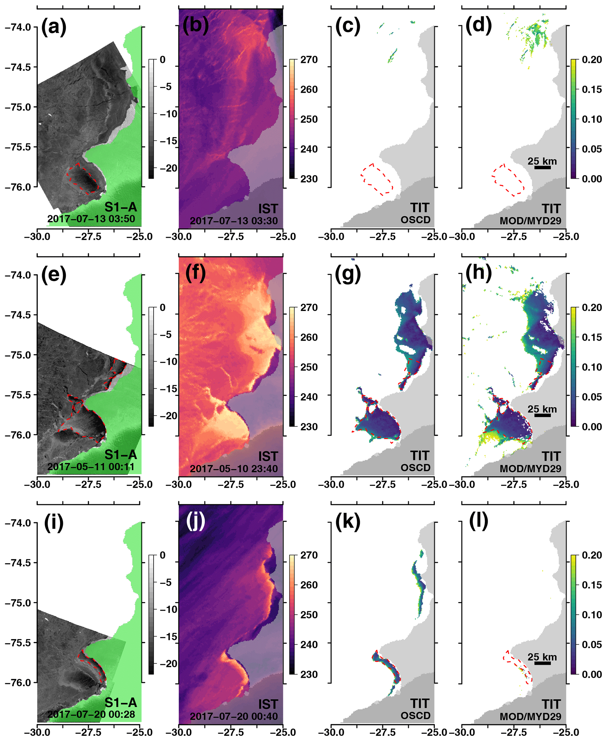
Figure 4Compilation of exemplary co-located S1-A/B calibrated backscatter (in dB) and MODIS swaths of ice-surface temperature (IST; in K) and derived thin-ice thickness (TIT; in m) data (Table 3). Gray and green overlays highlight the ice-shelf extent. Manually picked S1-A/B reference polynya extent is outlined by a dashed red line in all panels. Please note that the date format in this figure is year month day (yyyy-mm-dd).
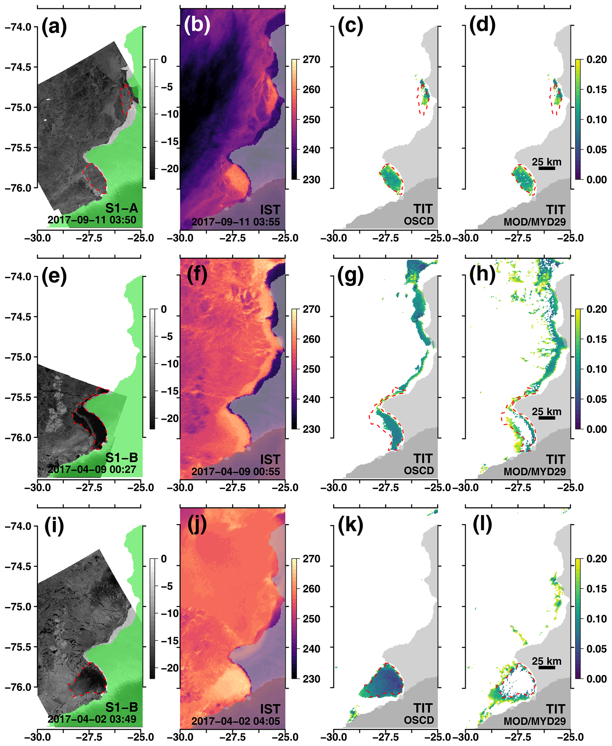
Figure 5Additional compilation of exemplary co-located S1-A/B and MODIS swaths in the same setup as Fig. 4. Gray and green overlays highlight the ice-shelf extent. Manually picked S1-A/B reference polynya extent is outlined by a dashed red line in all panels. Please note that the date format in this figure is year month day (yyyy-mm-dd).
Table 3Summary of polynya area (PA; in km2) estimates between S1-A/B (PAS1), OSCD (PAOSCD), and MOD/MYD29 (PAM29) data. PA estimates in parentheses correspond to the PA retrieved from MODIS for the S1-A/B polygon in Figs. 4 and 5.

3.1 Swath-based comparison
Representative comparisons between resulting the TIT from OSCD and MOD/MYD29 swaths reveal substantial differences, especially in the high-temperature polynya and thin-ice areas (PA; Figs. 4 and 5).
The S1-A/B reference data always feature a polynya signal in all our examples (Figs. 4a, e, and i and 5a, e, and i) and these are (at least partially) represented by a warm IST anomaly in the MODIS data (Figs. 4b, f, and j and 5b, f, and j). While for some examples the difference in resulting TIT between OSCD and MOD/MYD29 is comparably small or negligible (Figs. 4g and h and 5c and d), substantial differences appear for other examples (Figs. 4k and l, 5g and k, and 5h and l).
For a better comparison, the polynyas were hand-picked for the respective S1-A/B data in Figs. 4 and 5. The corresponding absolute polynya areas are summarized in Table 3. In addition to the respective numbers for each polynya, the corresponding area covered in the S1-A/B extent is given in parentheses. While there is some uncertainty due to the different grid resolutions (25 m vs. 1 km) as well as acquisition-time difference and subsequent changes due to sea-ice drift, this allows for a good quantification of the impact of erroneously classified cloud cover on the estimated TIT.
While there are correct and also corresponding cloud classifications in both MODIS products, the applied MODIS cloud mask in the MOD/MYD29 product tends towards additionally masking out strong positive temperature anomalies (Figs. 4l and 5h and l). This happens frequently in the center of the primary polynya around 27.4∘ W and 76∘ S and leads to substantial differences in PA estimates (Table 3).
Due to the strong temperature gradient between the warm ocean and the cold atmosphere, turbulent exchange of sensible and latent heat is large and can potentially lead to the formation of sea fog and thin, low cloud cover (Gultepe et al., 2003; Fraser et al., 2009). However, the temperature texture in the open-water and/or thin-ice areas appears to be homogeneous and is likely not to be affected by either sea fog or clouds to the extent suggested by the MOD/MYD29 product through the MODIS cloud mask.

Figure 6Daily polynya area difference in 103km2 using swath-wise pixel averages featuring a thin-ice thickness (TIT) ≤ 0.2 m between OSCD and MOD/MYD29. Difference is calculated by subtracting MOD/MYD29 from OSCD; results with OSCD ≥ MOD/MYD29 are shown in blue; results with OSCD < MOD/MYD29 are shown in red. Orange vertical bars highlight days with S1-A/B swath coverage used for calibration or training of the OSCD algorithm. Green vertical bars show additional S1-A/B swaths used for validation between products (Figs. 4 and 5). The top-left corner features a scatterplot of the daily polynya with MOD/MYD29 to OSCD. Additional information about the S1-A/B swaths is provided in Table 2.
3.2 Daily-composite-based comparison
Based on the median TIT of all available MODIS swaths per day, daily polynya area (PA) was computed (Paul et al., 2015), and the difference between OSCD and MOD/MYD29 was calculated (i.e., OSCD minus MOD/MYD29; Fig. 6).
Scattering of OSCD and MOD/MYD29 daily PA estimates against each other reveals a general tendency towards larger PA estimates in MOD/MYD29 data (Fig. 6; top-left scatterplot inlet). However, there is also a strong seasonality in this MOD/MYD29 bias, which dominates from 1 April 2017 to mid May 2017, while OSCD estimates are predominately larger than or equal to MOD/MYD29 between mid May and 30 September 2017 (Fig. 6). For the year 2017, about 64 %, 50.0 %, and 27 % of the differences of the absolute daily median PA are below 1000 km2, 500 km2, and 100 km2, respectively.
On average, OSCD estimates the daily polynya area (PA) between 1 April and 30 September 2017 to be 1.88 ×10³ km2 in contrast to 2.69 ×10³ km2 using MOD/MYD29 data (not shown). This corresponds to an average daily mean PA which is about 44 % smaller for OSCD compared to MOD/MYD29.
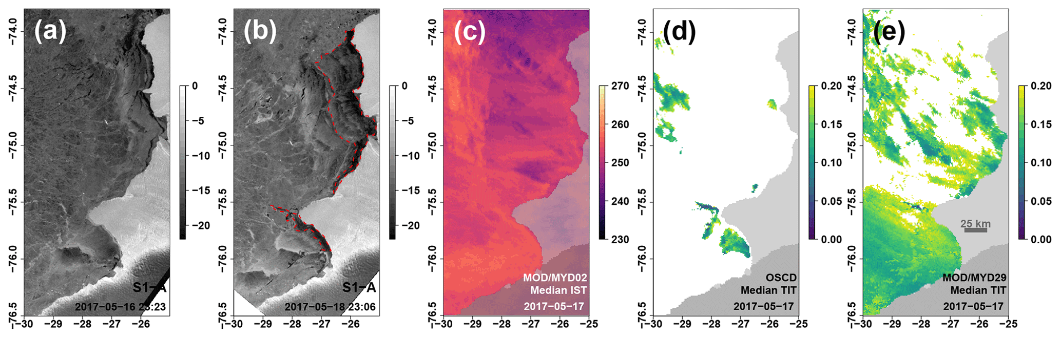
Figure 7Compilation of S1-A swaths acquired on 16 and 18 May 2017 (a, b, respectively; calibrated backscatter in dB), the daily median ice-surface temperature (IST; in K) composite for 17 May 2017 from all available MODIS swaths (c), and the resulting daily median thin-ice thickness (TIT; in m) composites for the OSCD (d) and MOD/MYD29 (e) products for 17 May 2017, respectively. Red dashed line outlines the polynya on 18 May 2017 in S1-A. Please note that the date format in this figure is year month day (yyyy-mm-dd).

Figure 8Compilation of MODIS swaths used for the computation of the data shown in Fig. 7: swath-based ice-surface temperature (IST in K; a–g), resulting swath-wise thin-ice thickness (TIT in m) using OSCD (h–n) and MOD/MYD29 (o–u) data, respectively. Please note that the date format in this figure is year month day (yyyy-mm-dd).
However, especially during freeze-up (i.e., between 1 April 2017 and mid May 2017), the differences are oftentimes very large (14.9 ×10³ km2 on 17 May 2017) and towards MOD/MYD29. To analyze this, we conduct a more detailed analysis of the OSCD and MOD/MYD29 daily median TIT (Figs. 7 and 8).
Unfortunately, no S1-A/B swath was acquired over the BIS area for 17 May 2017. However, S1-A/B swaths were acquired the day before and after (Table 2).
From the S1-A/B data (Fig. 7a and b), the existence of open water and/or thin ice very close to the ice-shelf edge around 27.4∘ W and 76∘ S for 18 May 2017 is evident.
The lack of any clearly distinguishable positive temperature-anomaly features in the MODIS daily median IST composite (Fig. 7c) and the general texture of rather smooth temperature patches are both signs for a persistently present cloud cover during 17 May 2017.
However, the relatively high temperatures of some of these potential clouds lead to an erroneous calculation of TIT and the subsequent daily median TIT composite with an erroneously much larger polynya area (PA) for MOD/MYD29 compared to OSCD (Fig. 7d and e). Nonetheless, also OSCD features TIT estimates from cloud artifacts in the northwest around 29.5∘ W and 74–74.5∘ S as well as in the area of the primary BIS polynya.
The individual swaths used for the computation of both composites underline the absence of any pronounced positive temperature anomalies corresponding to open-water and/or thin-ice features (Fig. 8a–g).
While cold clouds are reliably identified, the inability of the MODIS cloud mask to also reliably identify warm cloud patterns results in the computation of TIT in large patches west of BIS (Fig. 8q–u). Conversely, these false computations are not present or are at least much reduced in the OSCD data (Fig. 8j–n). However, while a small area west of the tip of the BIS around 28∘ W and 75.5∘ S corresponds well to the polynya signal in the S1-A data (Fig. 7b), the majority of the TIT estimates appear to be cloud artifacts (Fig. 8n).
From our analysis of the swath-based and daily-composite comparisons, three major take home messages can be summarized:
-
Erroneous TIT estimates due to (especially) warm cloud-cover artifacts resulting from false-negative classifications in the MOD/MYD29 data increase the overall estimated PA substantially. These false-negative classifications are reduced in the OSCD data.
-
False-positive cloud classifications over positive ice-surface temperature anomalies in the MOD/MYD29 data reduce the products' capability to estimate PA spatially and temporally correctly. These false-positive classifications are also reduced in the OSCD data.
-
Eliminating the thinnest sea-ice fraction of the thin-ice spectrum due to false-positive classifications potentially leads to a “thick” thin-ice bias during the daily-composite procedure.
The combined effect leads to spatially misplaced TIT estimates, likely not resolving the correct shape and (sub)daily thickness distribution of the open-water and/or thin-ice areas. Studies such as Paul et al. (2015) and Preußer et al. (2019), therefore, try to mitigate the effect of points 1 and 2 by introducing predefined masks.

Figure 9Comparison of per-pixel thin-ice occurrence based on all available swaths from 1 April to 30 September 2017 between the use of MOD/MYD29 (a) and OSCD data (b), respectively. White and green dashed lines mark the core BIS region as well as the primary BIS polynya area, respectively, used for further analyses.
3.3 Coverage comparison
In order to pick up on the last point, we would like to analyze the per-swath coverage in more detail, as this also influences the subdaily TIT distribution and, therefore, the thickness distribution of the resulting daily composite. It appears that the per-swath thin-ice occurrence frequency is much higher in the OSCD data compared to the MOD/MYD29 data (Fig. 9).
Quantifying the differences in the outlined subregions (Fig. 9; white and green dashed outlines), results in a 10 % and 20 % (BIS area and primary BIS polynya) higher detection rate of thin-ice pixels over all MODIS swaths between 1 April and 30 September 2017 in the OSCD data (Fig. 9b). This improved coverage likely leads to a higher-quality daily composite, as the impact from outliers is reduced. It admittedly sounds counterintuitive at first to have improved coverage (Fig. 9) with at the same time substantially less average PA (Fig. 6). This effect can be explained from the difference between swath and daily-composite data. Here, the increase in coverage mainly focuses around the primary polynya at BIS (green outline in Fig. 9). However, the substantial decrease in daily PA results from reducing the false-negative classifications of warm clouds as sea ice, primarily off the BIS edge to the west. These misclassification-related TIT estimates push the resulting average PA for the MOD/MYD29 data.
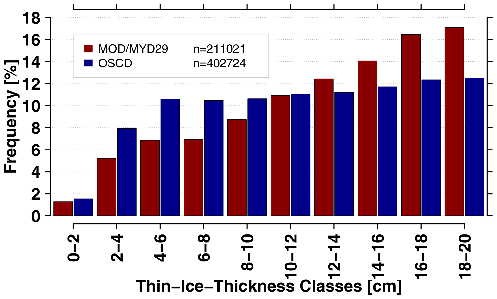
Figure 10Comparison of binned thin-ice thickness classes with a bin size of 2 cm based on all available swaths from 1 April to 30 September 2017 between the use of MOD/MYD29 (red) and OSCD (blue) data for the primary BIS polynya (green dashed outline in Fig. 9).
Based on our analysis in Sect. 3.1 and 3.2, we assumed that these additional thin-ice occurrences likely feature very thin ice, therefore, reducing the potential bias for thick thin sea ice in the MOD/MYD29 data. This is evident from Fig. 10. Here, the TIT occurrence frequency based on 2 cm bins for all available swaths between 1 April and 30 September 2017 is shown for the MOD/MYD29 and OSCD data. Thickness classes between 0 and 20 cm are much more frequent in the OSCD data (402 724; Fig. 10) compared to the MOD/MYD29 standard product (211 021; Fig. 10). The largest difference between both products, however, is the overall higher occurrence frequency of the thinnest ice fractions (between 0 and 10 cm) in the OSCD data compared to MOD/MYD29. As assumed before, there is a bias for thick thin ice present in the MOD/MYD29 data, which potentially plays an important role especially in the estimation of sea-ice production based on daily composites.
Despite great care during the manual categorization, uncertainty remains due to the lack of measured ground-truth data for the training data generation. However, the underlying statistical basis from the unsupervised FCM clustering in combination with a second stage of fully classifying all co-located MODIS swaths using NNs before generating the calibration or validation swath-split final training data for the OSCD algorithm appears to provide a realistic representation of the present sea-ice conditions in the BIS area.
In this study, we present a novel approach to improve the detection of wintertime cloud cover over Antarctic sea ice and its discrimination from sea-ice cover and open-water and/or thin-ice areas in MODIS thermal-infrared data using a deep neural network.
We established a labeled training data set using the techniques of dimension reduction, unsupervised clustering, and supervised learning in combination with manual visual screening and categorization. Through this effort, we generated a total of 13.1 ×10⁶ data points for 33 different predictors.
With this data set, we trained a deep neural network and used it to discriminate between open-water and/or thin-ice, sea-ice, and cloud-covered areas in the Brunt Ice Shelf region for the freezing period of 2017 (1 April to 30 September). Here, we computed the thin-ice thickness up to 0.2 m of open-water and/or thin-ice areas and evaluated the difference in daily polynya area and daily swath coverage to results using the standard NSIDC MOD/MYD29 sea-ice product.
Based on our approach, we obtain a 44 % lower average polynya area but 20 % higher swath coverage rate compared to the standard MOD/MYD29 product. On the one hand, the polynya area in MOD/MYD29 is likely dominated through frequent false-negative classifications of warm clouds as thin ice, leading to unrealistically large open-water and/or thin-ice areas, especially during freeze-up. On the other hand, the much lower coverage rate likely decreases the quality and accuracy of TIT estimates in the daily median TIT composites when using MOD/MYD29 data. Both factors are reduced in our OSCD data. This also reduces the impact of single outliers on the daily median TIT composites and, therefore, also increases the quality of derived information such as sea-ice production.
In the future, we plan to create an open-access comprehensive OSCD-based IST and TIT products covering all major Antarctic coastal polynyas, as well as providing higher-level parameters such as polynya area, sea-ice production, and associated ocean salt flux. We expect this data set to be of great use to the ocean–sea-ice–ice-shelf model community as well as for potential biological applications.
The generated initial training data set can be downloaded through Zenodo at https://doi.org/10.5281/zenodo.4596407 (Paul, 2021). Sources of all used data sets are referenced in the text.
SP designed the study and methodology, conducted the analysis, and wrote the original draft of the paper. MH assisted in the study design and the adaptation of the machine-learning algorithms as well as with writing the paper.
The authors declare no conflict of interests.
The authors want to thank the LAADS DAAC and the ASF DAAC for the provision of the MOD/MYD02 and S1-A/B data used here. The corresponding author appreciates the help of his family which enabled him to finally write this paper while working from home due to the SARS-CoV-2 pandemic. The comments by two anonymous reviewers as well as the editor, Claude Duguay, helped to substantially improve the quality of this paper.
The article processing charges for this open-access publication were covered by a Research Centre of the Helmholtz Association.
This paper was edited by Claude Duguay and reviewed by two anonymous referees.
Ackerman, S., Frey, R., Strabala, K., Liu, Y., Gumley, L., Baum, B., and Menzel, P.: MODIS Atmosphere L2 Cloud Mask Product, NASA MODIS Adaptive Processing System, Goddard Space Flight Center, Greenbelt, USA, https://doi.org/10.5067/MODIS/MOD35_L2.006, 2015. a
Adams, S., Willmes, S., Schröder, D., Heinemann, G., Bauer, M., and Krumpen, T.: Improvement and Sensitivity Analysis of Thermal Thin-Ice Thickness Retrievals, IEEE T. Geosci. Remote, 51, 3306–3318, 2013. a, b
Allaire, J. and Chollet, F.: keras: R Interface to “Keras”, r package version 2.3.0.0, available at: https://CRAN.R-project.org/package=keras, last access: 29 October 2020. a, b
Atkinson, P. M. and Tatnall, A. R. L.: Introduction Neural networks in remote sensing, Int. J. Remote Sens., 18, 699–709, https://doi.org/10.1080/014311697218700, 1997. a, b, c, d
Aulicino, G., Sansiviero, M., Paul, S., Cesarano, C., Fusco, G., Wadhams, P., and Budillon, G.: A New Approach for Monitoring the Terra Nova Bay Polynya through MODIS Ice Surface Temperature Imagery and Its Validation during 2010 and 2011 Winter Seasons, Remote Sens., 10, 366, https://doi.org/10.3390/rs10030366, 2018. a
Bezdek, J. C., Ehrlich, R., and Full, W.: FCM: The fuzzy c-means clustering algorithm, Comput. Geosci., 10, 191–203, https://doi.org/10.1016/0098-3004(84)90020-7, 1984. a
Cao, W., Wang, X., Ming, Z., and Gao, J.: A Review on Neural Networks with Random Weights, Neurocomput., 275, 278–287, https://doi.org/10.1016/j.neucom.2017.08.040, 2018. a, b, c
Dee, D. P., Uppala, S. M., Simmons, A. J., Berrisford, P., Poli, P., Kobayashi, S., Andrae, U., Balmaseda, M. A., Balsamo, G., Bauer, P., Bechtold, P., Beljaars, A. C. M., van de Berg, L., Bidlot, J., Bormann, N., Delsol, C., Dragani, R., Fuentes, M., Geer, A. J., Haimberger, L., Healy, S. B., Hersbach, H., Hólm, E. V., Isaksen, L., Kållberg, P., Köhler, M., Matricardi, M., McNally, A. P., Monge-Sanz, B. M., Morcrette, J.-J., Park, B.-K., Peubey, C., de Rosnay, P., Tavolato, C., Thépaut, J.-N., and Vitart, F.: The ERA-Interim reanalysis: configuration and performance of the data assimilation system, Q. J. Roy. Meteor. Soc., 137, 553–597, https://doi.org/10.1002/qj.828, 2011. a, b
Dong, G., Liao, G., Liu, H., and Kuang, G.: A Review of the Autoencoder and Its Variants: A Comparative Perspective from Target Recognition in Synthetic-Aperture Radar Images, IEEE T. Geosci. Remote, 6, 44–68, 2018. a
Drucker, R., Martin, S., and Moritz, R.: Observations of ice thickness and frazil ice in the St. Lawrence Island polynya from satellite imagery, upward looking sonar, and salinity/temperature moorings, J. Geophys. Res., 108, 3149, https://doi.org/10.1029/2001JC001213, 2003. a
Dunn, J. C.: A Fuzzy Relative of the ISODATA Process and Its Use in Detecting Compact Well-Separated Clusters, J. Cybernetics, 3, 32–57, https://doi.org/10.1080/01969727308546046, 1973. a
Fraser, A. D., Massom, R. A., and Michael, K. J.: A Method for Compositing Polar MODIS Satellite Images to Remove Cloud Cover for Landfast Sea-Ice Detection, IEEE T. Geosci. Remote, 47, 3272–3282, https://doi.org/10.1109/TGRS.2009.2019726, 2009. a, b
Fraser, A. D., Massom, R. A., and Michael, K. J.: Generation of high-resolution East Antarctic landfast sea-ice maps from cloud-free MODIS satellite composite imagery, Remote Sens. Environ., 114, 2888–2896, 2010. a
Fraser, A. D., Massom, R. A., Ohshima, K. I., Willmes, S., Kappes, P. J., Cartwright, J., and Porter-Smith, R.: High-resolution mapping of circum-Antarctic landfast sea ice distribution, 2000–2018, Earth Syst. Sci. Data, 12, 2987–2999, https://doi.org/10.5194/essd-12-2987-2020, 2020. a
Frey, R. A., Ackerman, S. A., Liu, Y., Strabala, K. I., Zhang, H., Key, J. R., and Wang, X.: Cloud Detection with MODIS. Part I: Improvements in the MODIS Cloud Mask for Collection 5, J. Atmos. Ocean. Tech., 25, 1057–1072, https://doi.org/10.1175/2008JTECHA1052.1, 2008. a
Goodfellow, I., Bengio, Y., and Courville, A.: Deep Learning, MIT Press, available at: http://www.deeplearningbook.org (last access: 18 January 20201), 2016. a, b, c, d
Gultepe, I., Isaac, G. A., Williams, A., Marcotte, D., and Strawbridge, K. B.: Turbulent heat fluxes over leads and polynyas, and their effects on arctic clouds during FIRE.ACE: Aircraft observations for April 1998, Atmos. Ocean, 41, 15–34, https://doi.org/10.3137/ao.410102, 2003. a
Hall, D., Key, J., Casey, K., Riggs, G., and Cavalieri, D.: Sea ice surface temperature product from MODIS, IEEE T. Geosci. Remote, 42, 1076–1087, https://doi.org/10.1109/TGRS.2004.825587, 2004. a, b, c
Hall, D. K. and Riggs, G. A.: MODIS/Terra Sea Ice Extent 5-min L2 Swath 1km, Version 6, National Snow and Ice Data Center, https://doi.org/10.5067/MODIS/MOD29.006, 2015a. a
Hall, D. K. and Riggs, G. A.: MODIS/Aqua Sea Ice Extent 5-min L2 Swath 1km, Version 6, National Snow and Ice Data Center, https://doi.org/10.5067/MODIS/MYD29.006, 2015b. a
Hall, D. K., Nghiem, S. V., Rigor, I. G., and Miller, J. A.: Uncertainties of Temperature Measurements on Snow-Covered Land and Sea Ice from In Situ and MODIS Data during BROMEX, J. Appl. Meteor. Climatol., 54, 966–978, https://doi.org/10.1175/JAMC-D-14-0175.1, 2015. a
Hall-Beyer, M.: Practical guidelines for choosing GLCM textures to use in landscape classification tasks over a range of moderate spatial scales, Int. J. Remote Sens., 38, 1312–1338, https://doi.org/10.1080/01431161.2016.1278314, 2017. a, b
Haralick, R. M.: Statistical and structural approaches to texture, Proc. IEEE, 67, 786–804, 1979. a
Haralick, R. M., Shanmugam, K., and Dinstein, I.: Textural Features for Image Classification, IEEE T. Syst. Man Cyb., 3, 610–621, 1973. a, b
Hartigan, J. A. and Wong, M. A.: Algorithm AS 136: A K-Means Clustering Algorithm, J. R. Stat. Soc. C-Appl., 28, 100–108, 1979. a
Holz, R. E., Ackerman, S. A., Nagle, F. W., Frey, R., Dutcher, S., Kuehn, R. E., Vaughan, M. A., and Baum, B.: Global Moderate Resolution Imaging Spectroradiometer MODIS cloud detection and height evaluation using CALIOP, J. Geophys. Res., 113, D00A19, https://doi.org/10.1029/2008JD009837, 2008. a
Kingma, D. P. and Ba, J.: Adam: A method for stochastic optimization, arXiv [preprint], arXiv:1412.6980, 30 January 2017. a, b
Kohonen, T.: An introduction to neural computing, Neural Networks, 1, 3–16, https://doi.org/10.1016/0893-6080(88)90020-2, 1988. a, b, c
LeCun, Y., Bengio, Y., and Hinton, G.: Deep learning, Nature, 521, 436–444, https://doi.org/10.1038/nature14539, 2015. a, b
Lee, J., Weger, R. C., Sengupta, S. K., and Welch, R. M.: A neural network approach to cloud classification, IEEE T. Geosci. Remote, 28, 846–855, 1990. a, b, c
Liu, Y. and Key, J. R.: Less winter cloud aids summer 2013 Arctic sea ice return from 2012 minimum, Environ. Res. Lett., 9, 044002, https://doi.org/10.1088/1748-9326/9/4/044002, 2014. a
Liu, Y., Key, J. R., Frey, R. A., Ackerman, S. A., and Menzel, W.: Nighttime polar cloud detection with MODIS, Remote Sens. Environ., 92, 181–194, https://doi.org/10.1016/j.rse.2004.06.004, 2004. a
Ludwig, V., Spreen, G., Haas, C., Istomina, L., Kauker, F., and Murashkin, D.: The 2018 North Greenland polynya observed by a newly introduced merged optical and passive microwave sea-ice concentration dataset, The Cryosphere, 13, 2051–2073, https://doi.org/10.5194/tc-13-2051-2019, 2019. a
MacQueen, J.: Some methods for classification and analysis of multivariate observations, Berkeley Symposium on Mathematical Statistics and Probability, 5.1, 281–297, 1967. a
Meyer, D., Dimitriadou, E., Hornik, K., Weingessel, A., and Leisch, F.: e1071: Misc Functions of the Department of Statistics, Probability Theory Group (Formerly: E1071), TU Wien, r package version 1.7-2, available at: https://CRAN.R-project.org/package=e1071 (last access: 14 October 2020), 2019. a
MODIS Characterization Support Team (MCST): MODIS 1km Calibrated Radiances Product, NASA MODIS Adaptive Processing System, Goddard Space Flight Center, Greenbelt, USA, https://doi.org/10.5067/MODIS/MYD021KM.06, 2017a. a, b
MODIS Characterization Support Team (MCST): MODIS 1km Calibrated Radiances Product, NASA MODIS Adaptive Processing System, Goddard Space Flight Center, Greenbelt, USA, https://doi.org/10.5067/MODIS/MYD021KM.06, 2017b. a, b
Paul, S.: Manually categorized initial training data for open-water/sea-ice/cloud discrimination (Version 1.0.0) [Data set], Zenodo, https://doi.org/10.5281/zenodo.4596407, 2021. a
Paul, S., Willmes, S., and Heinemann, G.: Long-term coastal-polynya dynamics in the southern Weddell Sea from MODIS thermal-infrared imagery, The Cryosphere, 9, 2027–2041, https://doi.org/10.5194/tc-9-2027-2015, 2015. a, b, c, d
Preußer, A., Ohshima, K. I., Iwamoto, K., Willmes, S., and Heinemann, G.: Retrieval of Wintertime Sea Ice Production in Arctic Polynyas Using Thermal Infrared and Passive Microwave Remote Sensing Data, J. Geophys. Res.-Oceans, 124, 5503–5528, https://doi.org/10.1029/2019JC014976, 2019. a, b
R Core Team: R: A Language and Environment for Statistical Computing, R Foundation for Statistical Computing, Vienna, Austria, available at: https://www.R-project.org/ (last access: 19 November 2020), 2018. a
Reiser, F., Willmes, S., and Heinemann, G.: A New Algorithm for Daily Sea Ice Lead Identification in the Arctic and Antarctic Winter from Thermal-Infrared Satellite Imagery, Remote Sens., 12, 1957, https://doi.org/10.3390/rs12121957, 2020. a
Riggs, G. and Hall, D.: MODIS Sea Ice Products User Guide to Collection 6, National Snow and Ice Data Center, University of Colorado, Boulder, USA, 50 pp., 2015. a, b, c, d
Schaffer, J., Timmermann, R., Arndt, J. E., Kristensen, S. S., Mayer, C., Morlighem, M., and Steinhage, D.: A global, high-resolution data set of ice sheet topography, cavity geometry, and ocean bathymetry, Earth Syst. Sci. Data, 8, 543–557, https://doi.org/10.5194/essd-8-543-2016, 2016. a, b, c
Schmidhuber, J.: Deep learning in neural networks: An overview, Neural Networks, 61, 85–117, https://doi.org/10.1016/j.neunet.2014.09.003, 2015. a, b
Toller, G., Xu, G., Kuyper, J., Isaacman, A., and Xiong, J.: MODIS Level 1B Product User’s Guide, NASA/Goddard Space Flight Center, Greenbelt, USA, 63 pp., 2009. a
Welch, R. M., Sengupta, S. K., Goroch, A. K., Rabindra, P., Rangaraj, N., and Navar, M. S.: Polar Cloud and Surface Classification Using AVHRR Imagery: An Intercomparison of Methods, J. Appl. Meteorol., 31, 405–420, http://www.jstor.org/stable/26186465 (last access: 22 October 2020), 1992. a, b, c
Yu, Y. and Rothrock, D. A.: Thin ice thickness from satellite thermal imagery, J. Geophys. Res., 101, 25753–25766, https://doi.org/10.1029/96JC02242, 1996. a
Zvoleff, A.: glcm: Calculate Textures from Grey-Level Co-Occurrence Matrices (GLCMs), r package version 1.6.4, available at: https://CRAN.R-project.org/package=glcm (last access: 29 October 2020), 2019. a, b