the Creative Commons Attribution 4.0 License.
the Creative Commons Attribution 4.0 License.
 | 11 Mar 2021
Estimating parameters in a sea ice model using an ensemble Kalman filter
Yong-Fei Zhang
Cecilia M. Bitz
Jeffrey L. Anderson
Nancy S. Collins
Timothy J. Hoar
Kevin D. Raeder
Edward Blanchard-Wrigglesworth
Uncertain or inaccurate parameters in sea ice models influence seasonal predictions and climate change projections in terms of both mean and trend. We explore the feasibility and benefits of applying an ensemble Kalman filter (EnKF) to estimate parameters in the Los Alamos sea ice model (CICE). Parameter estimation (PE) is applied to the highly influential dry snow grain radius and combined with state estimation in a series of perfect model observing system simulation experiments (OSSEs). Allowing the parameter to vary in space improves performance along the sea ice edge but degrades in the central Arctic compared to requiring the parameter to be uniform everywhere, suggesting that spatially varying parameters will likely improve PE performance at local scales and should be considered with caution. We compare experiments with both PE and state estimation to experiments with only the latter and have found that the benefits of PE mostly occur after the data assimilation period, when no observations are available to assimilate (i.e., the forecast period), which suggests PE's relevance for improving seasonal predictions of Arctic sea ice.
- Article
(1821 KB) - Full-text XML
-
Supplement
(2084 KB) - BibTeX
- EndNote


Arctic sea ice has undergone rapid decline in recent decades in all seasons (e.g., Stroeve et al., 2012; Serreze and Stroeve, 2015). The frequent large deviations of Arctic sea ice cover from its climatology and the impact of sea ice cover on the overlying atmosphere and on ocean–atmosphere fluxes motivate including an active sea ice component in seasonal-to-sub-seasonal (S2S) weather forecasts (Vitart et al., 2015). The persistence and reemergence of sea ice thickness (SIT) and sea surface temperature anomalies are major sources of predictability for Arctic sea ice extent (SIE; Blanchard-Wrigglesworth et al., 2011). Previous studies have demonstrated the importance of accurate initial conditions, especially SIT, in predicting Arctic sea ice extent (Day et al., 2014). Hence studies applying data assimilation (DA) techniques to fuse observations with model simulations are actively investigated (e.g., Lisæter et al., 2003; Chen et al., 2017; Massonnet et al., 2015), most of which are focused on improving model states only, not the parameters in sea ice parameterization schemes.
Sea ice models, like other components of Earth system models, can suffer large uncertainties originating from uncertain parameters. The widely used Los Alamos sea ice model version 5 (CICE5), given its various complex schemes, has hundreds of uncertain parameters, such as in the Delta-Eddington shortwave radiation scheme (Briegleb and Light, 2007). The default values of these parameters are usually chosen based on point measurements that are taken on multi-year sea ice (Light et al., 2008). Urrego-Blanco et al. (2015) conducted an uncertainty quantification study of CICE5 and ranked the parameters based on the sensitivities of model predictions to a list of parameters. This work provides guidance on which parameters could be estimated using an objective method and during which seasons. Their findings suggest that the estimates of the Arctic sea ice area and extent are especially sensitive to certain parameters (e.g., snow conductivity and snow grain size) in summer. However, they also discussed that their sensitivities could be low as a consequence of prescribing atmospheric forcing in their model setup, so parametric uncertainties are expected to be larger year-round (particularly in winter) in a fully coupled model. Previous studies suggest that the ensemble spread of sea ice states is generally small in winter (e.g., Lisaeter et al., 2003; Fritzner et al., 2018; Zhang et al., 2018), which will lead to limited update on model state variables or parameters. Also, sea ice concentration (SIC) reaches 100 % in most of regions in winter and hence does not leave enough room for improvements by DA. The ensemble spread in summer, however, is much larger. Since we run stand-alone CICE5 given that our aim is to demonstrate the utility of parameter estimation (PE) for sea ice, we conduct DA experiments with PE in summer.
Two types of observations are assimilated in our study, sea ice concentration and thickness (SIC and SIT, respectively). Satellite-retrieved SIC observations are widely utilized in the sea ice DA community, while the application of SIT observations is more challenging given its large uncertainty and lack of data in summer (Zygmuntowska et al., 2014). Previous studies on Arctic sea ice predictability emphasized the importance of summer SIT observations (e.g., Day et al., 2014; Dirkson et al., 2017). We explore the benefits of SIT observations (in addition to SIC) on sea ice parameter estimation and advocate the need to extend the data coverage of SIT observations into late spring and summer, which is actually possible in ICESat-2 (Kwok et al., 2020).
Despite the importance of sea ice model parameters, few studies have tried to estimate or reduce the parametric uncertainties, partly due to the large effort and computational cost if parameter calibration is done in a trial-and-error fashion. A more systematic way is through DA. Anderson (2002) demonstrated the feasibility of updating parameters using an ensemble filter in a low-order model. Annan et al. (2005) were among the first to apply an ensemble filter to estimate parameters in a complex Earth system model. Massonnet et al. (2014) employed the ensemble Kalman filter (EnKF) in a sea ice model to estimate three parameters that control sea ice dynamics. In addition to achieving their goal of improving the sea ice drift, they also realized slight improvements in the SIT distribution and extent as well as in the sea ice export through the Fram Strait.
Our purpose is to expand upon previous studies to explore the feasibility of optimizing sea ice parameters by asking how different observations (concentration and thickness in this study) would constrain the parameters differently, whether we need to allow parameters to vary spatially, and what the benefits are of the updated parameters both when observations are available for assimilation (the DA period) and when observations are not available (the forecast period).
We use CICE5 linked to the Data Assimilation Research Testbed (DART) (Anderson et al., 2009) within the framework of the Community Earth System Model version 2 (CESM2) (http://www.cesm.ucar.edu/models/cesm2, last access: May 2019). The ocean is modeled as a slab ocean, and the atmospheric forcing is prescribed from a DART/CAM ensemble reanalysis (Raeder et al., 2012). Details of this framework can be found in Zhang et al. (2018). The default DART/CICE framework is only used for state estimation; we extend DART/CICE to include parameter estimation in this study. During the assimilation, DART and CICE5 cycle between a DA step with DART and a 1 d forecast step with CICE5. During the DA step, the selected sea ice variables are placed into a “DART state vector” that is to be passed to the filter. The DART state vector is augmented by adding selected sea ice parameters, so that the parameters and state variables are both updated by the filter in the same way. The updated state variables are then post-processed (if needed) and sent with the updated parameters back to CICE5 for the next 1 d forecast step. The post-process step is necessary when the updated variable goes beyond its physical boundaries, for example, when SIC is negative or larger than 100 %. Unlike state variables, the parameters are not modified during CICE5 forecast steps.
The parameter we select, Rsnw, represents the standard deviation of dry snow grain radius that controls the optical properties of snow and is one of the key parameters that determine snow albedo in the Delta-Eddington solar radiation parameterization treatment (Briegleb and Light, 2007). We pick Rsnw because it is one of the parameters that the model predictions are sensitive to (Urrego-Blanco et al., 2016) and is also one of the parameters perturbed to generate ensemble spread in Zhang et al. (2018). Instead of directly tuning snow albedo that could result in inconsistencies with the rest of the parameterization scheme, tuning Rsnw changes the inherent optical properties of snow in a self-consistent fashion (Briegleb and Light, 2007). Increasing Rsnw leads to smaller dry snow grain radius and larger snow albedo (Hunke et al., 2015). The default value of Rsnw is 1.5, which corresponds to a fresh snow grain radius of 125 µm (Holland et al., 2012). Many parameters in CICE5, like Rsnw, have default values based on limited field observations. As sea ice models increase in complexity, empirical parameters will increasingly need to be calibrated objectively. More comprehensive observations at a large scale will presumably benefit a better representation of snow and ice properties in sea ice models.
The configurations of conducted experiments are listed in Table 1. We begin with a free run of CICE5 without DA (hereafter FREE) with 30 ensemble members. Each ensemble member has a unique value of Rsnw, which is constant in time and space. The ensemble of Rsnw values is randomly drawn from a uniform distribution spanning −2 to 2. One of the ensemble members is designated as the truth with the true value of Rsnw. Following Zhang et al. (2018), synthetic observations are created by adding random noise to SIC and SIT taken from the truth ensemble member. The noise follows a normal distribution with zero mean and a standard deviation of 15 % for SIC and 40 cm for SIT. The FREE experiment does not assimilate any observations, and the Rsnw values stay the same throughout the experimental period.
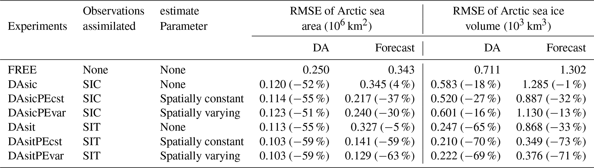
Table 1List of experiments with different configurations and RMSE of the total Arctic sea ice area and volume calculated over two experiment periods: DA (April to October 2005) and forecast (April to September 2006) for the seven experiments. All the experiments use the same localization half-width and prior inflation algorithm as stated in Sect. 3.
We then conduct two pairs of experiments to test the feasibility of estimating parameters using the ensemble adjustment Kalman filter (EAKF) (Anderson, 2002), which is a deterministic ensemble square root filter. Each experiment assimilates daily SIC or SIT synthetic observations. The first pair is referred to as DAsicPEcst and DAsitPEcst, with the former assimilating SIC observations and the latter SIT observations. In the first pair, each ensemble member has a unique spatially uniform Rsnw. The second pair is referred to as DAsicPEvar and DAsitPEvar, which has a separate value of Rsnw at each horizontal grid point. The augmented state has the single parameter for Rsnw in the first pair or the two-dimensional grid of Rsnw parameters in the second pair.
All variables in the sea ice state vector are two-dimensional in space. The parameter Rsnw and the state variables were updated based on their correlations with neighboring observations. The posterior ensemble generated by DART is always spatially varying. For the first pair of experiments, we take an area-weighted average of the two-dimensional posterior to get a spatially invariant Rsnw to send back to CICE5. For the second pair of experiments, the spatially varying posterior Rsnw was sent to CICE5. In all experiments, the sea ice component is run for 1 d to produce a new state that is augmented with the posterior Rsnw of the previous DA step. To increase the prior ensemble spread of Rsnw, a spatially and temporally adaptive inflation was applied to the priors of both the model states and Rsnw before they are sent to the filter (Anderson, 2007). The initial value, standard deviation, and inflation damping value of the adaptive inflation are 1.0, 0.6, and 0.9, respectively. The localization half-width is 0.01 radians (about 64 km) as discussed in Zhang et al. (2018). We also reject observations that are 3 standard deviations of the expected difference away from the ensemble mean of the forecast.
A third pair of experiments is conducted with only state DA (no parameter estimation), known as DAsic and DAsit, which assimilate daily SIC and SIT synthetic observations, respectively. DAsic and DAsit have the same ensemble set of Rsnw, which is also the initial set of Rsnw in the above PE experiments. The ensemble of Rsnw remains fixed throughout the experiment period.
All experiments begin on 1 April 2005 and run for 18 months. Synthetic observations are assimilated only during the first 6 months (the DA period), and the next 12 months are a pure forecast period to mimic the real-world situation when making a forecast. The values of Rsnw hold constant once DA ceases. We do not perform DA beyond October 2005 for two reasons. First, sea ice states have small ensemble spread in winter, as illustrated in Fig. 1a, so DA updates tend to be small. In contrast, the relatively larger spread from April to October ensures that assimilating observations can have more impact in updating model state variables and parameters. Second, the snow albedo feedback only influences the sea ice state when sunlight is present.

Figure 1Time series of (a) the Arctic sea ice area and (b) sea ice volume from a free CICE5 run. Each gray line represents one ensemble member, black line the ensemble mean, and red line the truth. Time series of (c) the parameter Rsnw for two DA experiments. Blue line represents DAsicPEcst that assimilates SIC observations, and magenta represents DAsitPEcst that assimilates SIT. The red reference line indicates the true value of Rsnw. Each error bar represents 2 standard deviations of the 30 ensemble members of Rsnw. Error bar is shown for every 5 d.
Several commonly used error indices are calculated to evaluate the performance of the experiments. The root-mean-square error (RMSE) of Arctic SIE and the area-weighted spatially averaged root-mean-square error (RMSEt) are defined as follows:
where i and j are the indices in time and space, x refers to Arctic SIE in RMSE and may refer to parameters or model states in RMSEt, N is the number of days, and M is the number of grid cells. The superscripts m and t refer to model and truth, respectively. The overbar indicates the mean of the model ensemble.
Model bias is defined as the mean of the 30-member ensemble of the experiments minus the truth. Absolute bias difference (ABD) between two experiments is defined as follows:
where x may refer to parameters or model states, the superscripts t refers to the truth, and case1 and case2 refer to the two experiments to compare. The overbar indicates the mean of the model ensemble.
4.1 Temporally and spatially invariant parameters
The ensemble mean of FREE underestimates SIC throughout the year (Fig. 1a) partly because our arbitrary ensemble member selected as the truth has an above-average Rsnw (Fig. 1c). As such, we would intuitively expect Rsnw to have a positive increment as a result of assimilating SIC observations. Figure 1c confirms that Rsnw increments are positive, with the posterior ensemble mean gradually approaching the true value during the DA period in the spatially constant PE experiments (DAsicPEcst and DAsitPEcst). The posterior Rsnw has smaller ensemble spread than the prior Rsnw (also see Fig. S1d, e, and f), which is consistent with the EAKF theory. In Fig. 1c DAsitPEcst outperforms DAsicPEcst starting in June, indicating that SIT provides more information than SIC for Rsnw. Similarly, with state-only DA, Zhang et al. (2018) found that SIT is more efficient than SIC observations at constraining state variables. There could be several reasons why the rate at which Rsnw approaches the true value decreases with time. First, the ensemble spread of Rsnw may be insufficient because no uncertainty is introduced into Rsnw in CICE5 during the forecast step. It is an open question how much additional uncertainty should be introduced into the parameters. To help avoid filter divergence, we apply the prior adaptive inflation to the parameters (as well as to the model states), which may still be not enough. Second, the correlation between Rsnw and the observations may be too weak. Solar radiation becomes very low by the end of September, and hence Rsnw has little impact on sea ice, which explains the weak correlation between Rsnw and the observations (further discussed below). Either reason could result in a negligible update to Rsnw.
The correlations between Rsnw and the observations have unique spatial patterns and evolve with time. On 1 May, the correlation between Rsnw and SIC is generally positive (Fig. 2a). The positive correlations are significant especially where SIC is under ∼100 %. Larger Rsnw corresponds to higher snow albedo and more reflected sunlight, which in turn delays the melting of sea ice. The correlations are still significant along the ice edges in August (Fig. 2c) and become noisier and have less significant values by the end of the melt season (Fig. 2e). The correlation between Rsnw and SIT has different spatial patterns (Fig. S2b, d, and f). Negative correlations between Rsnw and SIT on 1 May can be seen in the Chukchi Sea, Beaufort Sea, and East Siberian Sea, where Rsnw and SIC have positive correlations. This suggests that where SIC increases with Rsnw in spring it is possible that SIT actually decreases, which might be due to elevated concentration raising the compressive strength and reducing sea ice deformation. While a brighter surface is able to reduce thickness over large regions in spring, the effect is mostly gone by the end of summer, when positive correlation prevails.
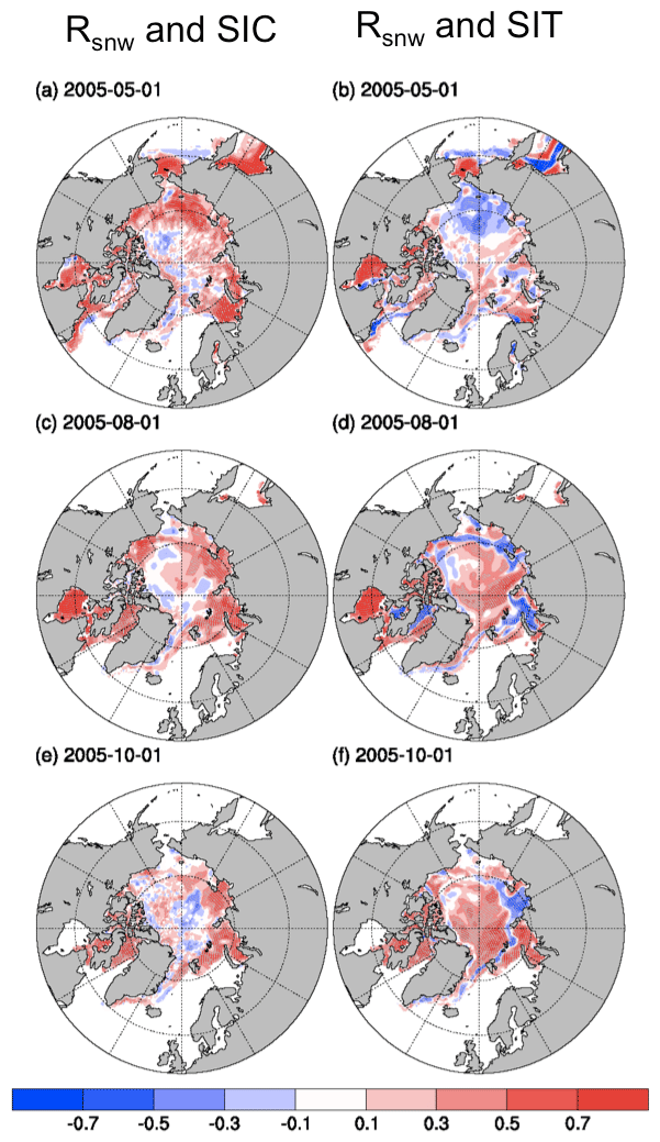
Figure 2Correlations between (a) Rsnw and SIC and (b) Rsnw and SIT for 1 May 2005, (c) Rsnw and SIC and (d) Rsnw and SIT for 1 August 2005, and (e) Rsnw and SIC and (f) Rsnw and SIT for 1 October 2005. At each point, we calculate the correlation of Rsnw and the observed quantities across the 30 ensemble members on the selected dates. The posterior states outputted from the experiments DAsicPEcst and DAsitPEcst are used for calculation.
4.2 Spatially varying Rsnw
We discussed in Sect. 4.1 that processes relating Rsnw and observed quantities have complex spatial features. The spatial map of the posterior Rsnw and the reduction in the ensemble spread of Rsnw after EAKF in the first pair of experiments (Fig. S1) also suggest that the updates are concentrated on the ice marginal zones. It may be too crude to use a single value of Rsnw for the whole Arctic. We let Rsnw be a spatially varying parameter in the second pair of PE experiments, even though the true Rsnw is spatially invariant. The spatial features of Rsnw will purely depend on how Rsnw correlates with the observations. As in DAsicPEcst and DAsitPEcst, the analysis field of Rsnw is spatially varying, and we did a spatial averaging to get a single number for the next run. Rsnw along the sea ice edges gets updated more, while Rsnw in the center is less influenced. But the averaging smoothed out this spatial feature. In DAsicPEvar and DAsitPEvar, we let the spatially varying 2D analysis field of Rsnw be the Rsnw field in the next run, so the spatial feature was carried along the simulation.
Figure 3 depicts the ABD of Rsnw (defined in Sect. 2) between different pairs of experiments at the end of the DA period. Figure 3a and d confirm that DAsicPEcst and DAsitPEcst improve the Rsnw compared to FREE. Figure 3b and e show the spatial feature of improvements or degradations in Rsnw for the two spatially varying PE experiments. They both show the contrast between the ice marginal zones and the central Arctic. Improvements are mostly seen along the ice edges. Spotty improvements in the inner Arctic can be found in DAsitPEvar (Fig. 3e), while degradations are prevailing in the inner Arctic in DAsicPEvar (Fig. 3b). Figure 3c and f highlight the improvements or degradations from allowing Rsnw to vary spatially. The general features are that DAsicPEvar and DAsitPEvar have reduced Rsnw biases more along the ice edges compared with DAsicPEcst and DAsitPEcst. However, degradations (Fig. 3c) or negligible improvements (Fig. 3f) are found in the central Arctic. This suggests that spatially invariant PE generally works better for the whole pan-Arctic regions, while spatially varying PE can work well in the ice marginal zones but not in the central Arctic, especially when SIC is the only observed quantity. SIC has little variability in the central Arctic, and hence assimilating the SIC observations will not add much information for parameters or model states. Besides the improvements along the sea ice edges, the SIT DA also has a benefit in the inner ice pack (Fig. 3e), which is consistent with the results of the first pair of experiments that SIT in general provides more information than the SIC observations, especially in the regions where SIC has little variability. However, spatially varying Rsnw has small advantages over spatially invariant Rsnw in the ice marginal regions but degradations in the central Arctic too (Fig. 3f). The degradations in Rsnw but improvements in SIC (Fig. 5a and c; discussed in Sect. 4.3) in the central Arctic suggest that Rsnw is likely over-adjusted to cancel out other errors (e.g., noise from atmospheric forcing fields).
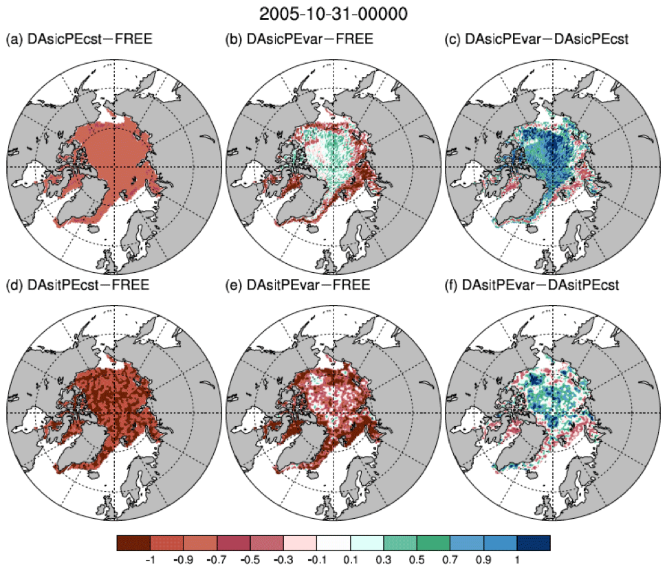
Figure 3The differences of absolute mean bias (ABD; see Eq. 2) of Rsnw between the DA experiments – (a) DAsicPEcst, (b) DAsicPEvar, (d) DAsitPEcst, and (e) DAsitPEvar – and the control experiment FREE, and between the spatially varying PE experiments and the spatially constant PE experiments: (c) DAsicPEvar and DAsicPEcst, and (f) DAsitPEvar and DAsitPEcst.
4.3 Additional improvements in model states
We demonstrated that Rsnw approaches the true value by assimilating SIC or SIT (at different rates) in the previous sections. We now investigate whether PE also improves the simulation of model states, beginning with time series of the pan-Arctic sea ice area and volume in all of our experiments (see Fig. 4).
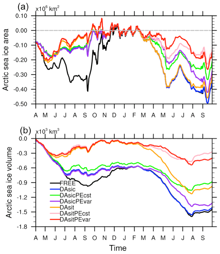
Figure 4Daily biases of (a) the total Arctic sea ice area and (b) the total Arctic sea ice volume for FREE (black), DAsic (blue), DAsicPEcst (green), DAsicPEvar (purple), DAsit (orange), DAsitPEcst (pink), and DAsitPEvar (red). Gray dash line in each plot represents the zero reference line. The blue line in panel (a) is overlapped by the purple and green lines in the first half of time. The black line in panel (a) is overlapped by the orange and blue lines in the second half of time. The black line in (b) is overlapped by the blue line from February to July.
In our preceding work, we showed that assimilating SIC and SIT could improve model states (Zhang et al., 2018), which can also be confirmed in Fig. 4. During the DA period, DAsic can efficiently reduce biases in area, but DAsic has limited influence on volume. Within about a month into the forecast period, DAsic improves neither area nor volume. In contrast, DAsit is highly beneficial at reducing both area and volume during the DA period, with at least some improvement to volume persisting through the whole 1-year forecast period.
We find that updating Rsnw has a relatively large impact on volume beginning in spring of the forecast period (Fig. 4b). Treating Rsnw as either a spatially varying or a constant parameter has about the same effect until late summer of the forecast period. In fact, all of the PE experiments outperform the state-only DA experiments in the forecast period. As shown in Table 1, SIT DA with PE always performs the best, reducing the bias in area by up to 63 % and reducing the bias in volume by up to 73 %. SIC DA with PE is second best in terms of simulating the area, reducing the bias by up to 37 %. SIC DA with PE is comparable to DAsit in simulating volume, reducing the bias by around 30 %.
Finally, we compare the spatial patterns of bias reduction in SIC and SIT from PE experiments by comparing RMSEt of SIT in DAsicPEcst and DAsitPEcst to their state-only DA counterparts, DAsic and DAsit (see Fig. 5). The comparisons are made in two periods: the DA period (April to October 2005) and the forecast period (April to September 2006). Zhang et al. (2018) showed that the DAsic could only improve SIT along the sea ice edges. Figure 5a demonstrates that DAsicPEcst offers some improvements in the central Arctic as well. Improvements that resulted from a more accurate Rsnw in the forecast period are more prominent (Fig. 5b). For DAsitPEcst, SIT is improved almost everywhere in the Arctic, with slight degradations along the ice edges (Fig. 5c). The improvements persist throughout the forecast period (Fig. 5d).
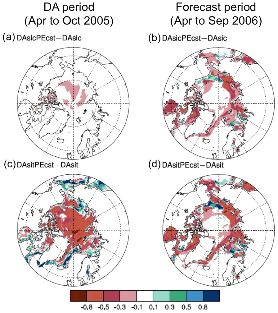
Figure 5The relative differences of RMSEt of SIT between DAsicPEcst and DAsic for the (a) DA experiment period and (b) forecast period, and between DAsitPEcst and DAsit for the (c) DA experiment period and (d) forecast period. The differences of RMSEt are divided by the RMSEt of DAsic and DAsit, respectively, to get the relative differences.
We extend the functionality of DART/CICE to do PE through the EAKF as well as updating the model states. One of the key parameters determining sea ice surface albedo, Rsnw, is estimated as an example in this study. Rsnw is updated using the filter. We designed a series of OSSEs to demonstrate the feasibility of PE in CICE5. Results show that Rsnw gradually approaches the true value during the DA period (from April to October 2005). Updating parameters with PE could further improve the model state estimation but not prominently in the DA period. During the forecast period, with a better representation of the parameter, the PE experiments show significant superiority over the state-only DA experiments, both in SIC and SIT. The results in the forecast period indicate that, by updating parameters as well as state variables, assimilating SIC observations only is comparable to assimilating SIT observations. We concluded that SIT is the most important variable to be observed in Zhang et al. (2018), but satellite observations of SIT have large uncertainties and only cover a short time period. We could alternatively improve model parameters by assimilating SIC observations, with the ultimate goal of improving SIT. Results from the subset of experiments treating Rsnw as a spatially varying parameter suggest that the Rsnw biases are mostly reduced along the sea ice edges but not as much in the central Arctic. We suggest that varying Rsnw spatially is not effective when conducting DA for the whole Arctic, but worth exploring when it comes to regional studies, such as in the seasonal sea ice zones.
Model data are available at https://doi.org/10.6084/m9.figshare.13670770 (Zhang et al., 2021).
The supplement related to this article is available online at: https://doi.org/10.5194/tc-15-1277-2021-supplement.
YFZ and CMB conceptualized the idea; YFZ, CMB, and JLA discussed the realization of the idea and experimental design; NSC, TJH, and KDR contributed to the software setup; and FYZ carried out the experiments and wrote the manuscript. CMB and EBW contributed to the discussion of the results. All co-authors contributed to the revisions of the paper.
The authors declare that they have no conflict of interest.
We thank Adrian Raftery and Hannah Director for helpful discussions, and David Bailey and Marika Holland for suggestions about choosing the proper parameters to estimate in the Los Alamos sea ice model. We acknowledge the Computational & Information Systems Lab at the National Center for Atmospheric Sciences and Texas Advanced Computer Center at The University of Texas at Austin for providing high-performance computing resources that have contributed to the research results reported within the paper.
This research has been supported by the NOAA (grant no. CPO NA15OAR4310161).
This paper was edited by Petra Heil and reviewed by two anonymous referees.
Anderson, J.: An ensemble adjustment Kalman filter for data assimilation, Mon. Weather Rev., 129, 2884–2903, 2002.
Anderson, J. L.: An adaptive covariance inflation error correction algorithm for ensemble filters, Tellus, 59, 210–224, 2007.
Anderson, J. L., Hoar, T., Raeder, K., Liu, H., Collins, N., Torn, R., and Arellano, A.: The Data Assimilation Research Testbed: Acommunity facility, B. Am. Meteor. Soc., 90, 1283–1296, https://doi.org/10.1175/2009BAMS2618.1, 2009.
Annan, J. D., Hargreaves, J. C., Edwards, N. R., and Marsh, R.: Parameter estimation in an intermediate complexity earth system model using an ensemble Kalman filter, Ocean Modell., 8, 135–154, https://doi.org/10.1016/j.ocemod.2003.12.004, 2005.
Blanchard-Wrigglesworth, E., Armour, K. C., Bitz, C. M., and deWeaver, E.: Persistence and inherent predictability of Arctic sea ice in a GCM ensemble and observations, J. Climate, 24, 231–250, https://doi.org/10.1175/2010JCLI3775.1, 2011.
Briegleb, B. P. and Light, B.: A Delta-Eddington mutiple scattering parameterization for solar radiation in the sea ice component of the Community Climate System Model, NCAR Technical Note NCAR/TN-472+STR, https://doi.org/10.5065/D6B27S71, 2007.
Chen, Z., Liu, J., Song, M., Yang, Q., and Xu, S.: Impacts of assimilating satellite sea ice concentration and thickness on Arctic sea ice prediction in the NCEP Climate Forecast System, J. Climate, 30, 8429–8446, 2017.
Day, J. J., Hawins E., and Tietsche, S.: Will Arctic sea ice thickness initialization improve seasonal forecast skill?, Geophys. Res. Lett., 41, 7566–7575, https://doi.org/10.1002/2014GL061694, 2014.
Dirkson, A., Merryfield, W. J., and Monahan, A.: Impacts of sea ice thickness initialization on seasonal Arctic sea ice pre- dictions, J. Climate, 30, 1001–1017, https://doi.org/10.1175/JCLI-D-16-0437.1, 2017.
Fritzner, S. M., Graversen, R. G., Wang, K., and Christensen, K. H.: Comparison between a multi-variate nudging method and the ensemble Kalman filter for sea-ice data assimilation, J. Glaciol., 64, 387–396, 2018.
Holland, M. M., Bailey, D. A., Briegleb, B. P., Light, B., and Hunke, E.: Improved sea ice shortwave radiation physics in CCSM4: The impact of melt ponds and aerosols on Arctic sea ice, J. Climate, 25, 1413–1430, https://doi.org/10.1175/JCLI-D-11-00078.1, 2012.
Hunke, E. C., Lipscomb, W. H., Turner, A. K., Jeffery, N., and Elliott, S.: CICE: The Los Alamos Sea ice model documentation and software user's manual version 5, Los Alamos National Laboratory, Los Alamos, NM, USA, 116 pp., 2015.
Kwok, R., Cunningham, G. F., Kacimi, S., Webster, M. A., Kurtz, N. T., and Petty, A. A.: Decay of the snow cover over Arctic sea ice from ICESat-2 acquisitions during summer melt in 2019, Geophys. Res. Lett., 47, e2020GL088209, https://doi.org/10.1029/2020GL088209, 2020.
Light, B., Grenfell, T. C., and Perovich, D. K.: Transmission and absorption of solar radiation by Arctic sea ice during the melt season, J. Geophys. Res., 113, C03023, https://doi.org/10.1029/2006JC003977, 2008.
Lisæter, K., Rosanova, J., and Evensen, G.: Assimilation of ice concentration in a coupled ice–ocean model, using the ensemble Kalman filter, Ocean Dyn., 53, 368–388, https://doi.org/10.1007/s10236-003-0049-4, 2003.
Massonnet, F., Goosse, H., Fichefet, T., and Counillon, F.: Calibration of sea ice dynamic parameters in an ocean-sea ice model using an ensemble Kalman filter, J. Geophys. Res.-Oceans, 119, 4168–4184, https://doi.org/10.1002/2013JC009705, 2014.
Massonnet F., Fichefet, T., and Goosse, H.: Prospects for improved seasonal Arctic sea ice predictions from multi-variate data assimilation, Ocean Modell., 28, 16–25, 2015.
Raeder, K., Anderson, J. L., Collins, N., Hoar, T. J., Kay, J. E., Lauritzen, P. H., and Pincus, R.: DART/CAM: an ensemble data assimilation system for CESM atmospheric models, J. Climate, 25, 6304–6317, 2012.
Serreze, M. C. and Stroeve, J.: Arctic sea ice trends, variability and implications for seasonal ice forecasting, Philos. T. Roy. Soc. A, 373, 20140159, https://doi.org/10.1098/rsta.2014.0159, 2015.
Stroeve, J. C., Kattsov, V., Barrett, A., Serreze, M., Pavlova, T., Holland, M., and Meier, W.: Trends in Arctic sea ice extent from CMIP5, CMIP3, and observations, Geophys. Res. Lett., 39, L16502, https://doi.org/10.1029/2012GL052676, 2012.
Urrego-Blanco, J. R., Urban, N. M., Hunke, E. C., Turner, A. K., and Jeffery, N.: Uncertainty quantification and global sensitivity analysis of the Los Alamos sea ice model, J. Geophys. Res.-Oceans, 121, 2709–2732, https://doi.org/10.1002/2015JC011558, 2016.
Vitart, F., Robertson, A. W., and S2S Steering Group: Sub-seasonal to seasonal prediction: Linking weather and climate, in: Seamless Prediction of the Earth System: From Minutes to Months, edited by: Brunet, G., Jones, S., and Ruti, P. M., WMO-1156, World Meteorological Organization, 385–401, 2015.
Zhang, Y., Bitz, C. M.; L. Anderson, J., Collins, N., Hoar, T. J., Raeder, K., and Blanchard-Wrigglesworth, E.: Estimating parameters in a sea ice model using an ensemble Kalman filter, figshare, Dataset, https://doi.org/10.6084/m9.figshare.13670770.v1, 2021.
Zhang, Y.-F., Bitz, C. M., Anderson, J. L., Collins, N., Hendricks, J., Hoar, T. J., and Raeder, K.: Insights on sea ice data assimilation from perfect model observing system simulation experiments, J. Climate, 5911–5926, https://doi.org/10.1175/JCLI-D-17-0904.1, 2018.
Zygmuntowska, M., Rampal, P., Ivanova, N., and Smedsrud, L. H.: Uncertainties in Arctic sea ice thickness and volume: new estimates and implications for trends, The Cryosphere, 8, 705–720, https://doi.org/10.5194/tc-8-705-2014, 2014.