the Creative Commons Attribution 4.0 License.
the Creative Commons Attribution 4.0 License.
 | 16 Mar 2020
Spatial and temporal variations in glacier aerodynamic surface roughness during the melting season, as estimated at the August-one ice cap, Qilian mountains, China
Junfeng Liu
Chuntan Han
The aerodynamic roughness of glacier surfaces is an important factor governing turbulent heat transfer. Previous studies rarely estimated spatial and temporal variation in aerodynamic surface roughness (z0) over a whole glacier and whole melting season. Such observations can do much to help us understand variation in z0 and thus variations in turbulent heat transfer. This study, at the August-one ice cap in the Qilian mountains, collected three-dimensional ice surface data at plot scale, using both automatic and manual close-range digital photogrammetry. Data were collected from sampling sites spanning the whole ice cap for the whole of the melting season. The automatic site collected daily photogrammetric measurements from July to September of 2018 for a plot near the center of the ice cap. During this time, snow cover gave way to ice and then returned to snow. z0 was estimated based on micro-topographic methods from automatic and manual photogrammetric data. Manual measurements were taken at sites from the terminals to the top of the ice cap; they showed that z0 was larger at the snow and ice transition zone than in areas that are fully snow or ice covered. This zone moved up the ice cap during the melting season. It is clear that persistent snowfall and rainfall both reduce z0. Using data from a meteorological station near the automatic photogrammetry site, we were able to calculate surface energy balances over the course of the melting season. We found that high or rising turbulent heat, as a component of surface energy balance, tended to produce a smooth ice surface and a smaller z0 and that low or decreasing turbulent heat tended to produce a rougher surface and larger z0.
- Article
(14124 KB) - Full-text XML
- BibTeX
- EndNote


The roughness of ice surfaces is an important control on air–ice heat transfer, on the ice surface albedo, and thus on the surface energy balance (Greuell and Smeets, 2001; Hock and Holmgren, 2005; Irvine-Fynn et al., 2014; Steiner et al., 2018). The snow and ice surface roughness at centimeter and millimeter scales is also an important parameter in studies of wind transport, snowdrifts, snowfall, snow grain size and ice surface melt (Denby and Smeets, 2000; Brock et al., 2006; McClung and Schaerer, 2006; Fassnacht et al., 2009a, b). Radar sensor signals, such as Synthetic Aperture Radar (SAR) (Oveisgharan and Zebker, 2007), altimeters and scatter meters, are also affected by ice and snow surface roughness (Lacroix et al., 2007, 2008). One of the most important of these influences is the aerodynamic roughness of z0, which is related to ice surface topographic roughness in a complex way (Andreas, 2002; Lehning et al., 2002; Smith, 2014; Smith et al., 2016). Determination of z0 based on topographic roughness is therefore of great interest for energy balance studies (Greuell and Smeets, 2001).
Glacier surface z0 has been widely studied through methods such as eddy covariance (Munro, 1989; Smeets et al., 2000; Smeets and Van den Broeke, 2008; Fitzpatrick et al., 2019) or wind profiling (Wendler and Streten, 1969; Greuell and Smeets, 2001; Denby and Snellen, 2002; Miles et al., 2017; Quincey et al., 2017). However, micro-topographic estimated z0 shows some advantages, such as lower scatter compared to profile measurements over slush and ice (Brock et al., 2006), and ease of application at different locations (Smith et al., 2016). Current research has increasingly used the micro-topographic method to estimate z0. It has also become clear that it is important to estimate z0 over the entire course of the melting season and at many points on the glacier surface, as z0 is prone to large spatial and temporal variation (Brock et al., 2006; Smeets and Van den Broeke, 2008). This variation is due to variations in weather and snowfall (Albert and Hawley, 2002). The micro-topographic estimated z0 allows repeated measurement at many points on the glacier surface, which is not possible with wind profile or eddy covariance methods.
Photogrammetry has been increasingly popular as a method to measure the aerodynamic surface roughness of snow and ice (Irvine-Fynn et al., 2014; Smith et al., 2016; Miles et al., 2017; Quincey et al., 2017; Fitzpatrick et al., 2019). Initially, the micro-topographic method was developed because snow digital photos were taken against a dark background plate. The contrast between the surface photo and the plate could then be quantified as a measure of glacier roughness (Rees, 1998). This method is still widely applied for quantifying glacier surface roughness (Rees and Arnold, 2006; Fassnacht et al., 2009a, b; Manninen et al., 2012). A more recent method, as described by Irvine-Fynn et al. (2014), uses modern consumer-grade digital cameras to do close-range photogrammetry at plot scale (small plots of only a few square meters). Appropriate image settings and acquisition geometry allow the collection of high-resolution data (Irvine-Fynn et al., 2014; Rounce et al., 2015; Smith et al., 2016; Miles et al., 2017; Quincey et al., 2017). Such data facilitates the distributed parameterization of aerodynamic surface roughness over glacier surfaces (Smith et al., 2016; Miles et al., 2017; Fitzpatrick et al., 2019). Precision of micro-topographic estimated z0 also became a major concern, and many comparative studies with the aerodynamic method (eddy covariance or wind towers measurements) were carried out over debris-covered or non-debris-covered glaciers. The difference was within an order of magnitude for some studies (Fitzpatrick et al., 2019) or strongly correlated (Miles et al., 2017).
Previous researchers have performed some long-term systematic studies of glacier surfaces (Smeets et al., 1999; Brock et al., 2006; Smeets and Van den Broeke, 2008; Smith et al., 2016). The current study applied such methods to the study of snow and ice aerodynamic surface roughness during the melting season at the August-one ice cap. We used both automatic digital photogrammetry and manual photogrammetry. Automatic methods allowed us to monitor daily variations in aerodynamic surface roughness, and manual methods allowed us to characterize aerodynamic surface roughness variation along the main glacial flow line. We also recorded meteorological observations in order to study the impact of weather conditions (e.g., snowfall or rainfall) on aerodynamic surface roughness. This data allowed a further effort to characterize variation in plot-scale z0 from an energy balance perspective.

Figure 1Location of ice cap and study sites. (a) Location of the August-one glacier. (b) Locations of the AWS, automatic and manual photogrammetry plots, and shortwave observation platforms.
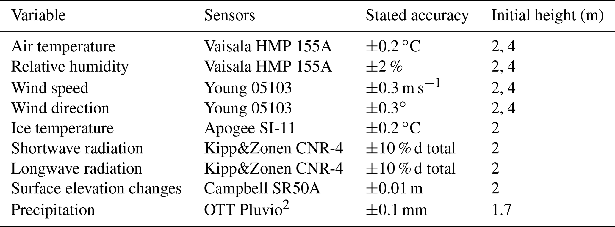
Table 1Measurement specifications for the AWS located at the top of the glacier (4820 m a.s.l.). The heights indicate the initial sensor distances to the glacier surface; the actual distances are derived from the SR50A sensor.
2.1 Study area and meteorological data
The August one glacier ice cap is located in the middle of Qilian Mountains on the northeastern edge of the Tibetan Plateau (Fig. 1a, b). The glacier is a flat-topped ice cap that is approximately 2.3 km long and 2.4 km2 in area. It ranges in elevation from 4550 to 4820 m a.s.l. (Guo et al., 2015). This study was conducted during the melting season of 2018, a season characterized by high precipitation. Energy balance analysis indicated that net radiation contributes 86 % and turbulent heat fluxes contribute about 14 % to the energy budget in the melting season. A sustained period of positive turbulent latent flux exists on the August one ice cap in August, causing faster melt rate in this period (Qing et al., 2018).
Researchers had access to meteorological data that had been recorded continuously since September 2015, when an automatic weather station (AWS) was sited at the top of the ice cap (Table 1). The AWS measures air temperature, relative humidity and wind speed at 2 and 4 m above the surface. Air pressure, incoming and reflected solar radiation, incoming and outgoing longwave radiation, and glacial surface temperature (using an infrared thermometer) are measured at 2 m height. Mass balance is measured by a Campbell Scientific ultrasonic depth gauge (UDG) close to the AWS. An all-weather precipitation gauge adjacent to the AWS measures solid and liquid precipitation. All sensors sample data every 15 s. Half-hourly means are stored on a data logger (CR1000, Campbell, USA). Throughout the entire melting season (from June to September) researchers periodically checked the AWS station to make sure that it remained horizontal and in good working order. During the entire study period, precipitation total was 261.3 mm, as measured at the AWS. Of this precipitation, 172.1 mm was snow or sleet and 89.2 mm was rainfall (Fig. 7a).
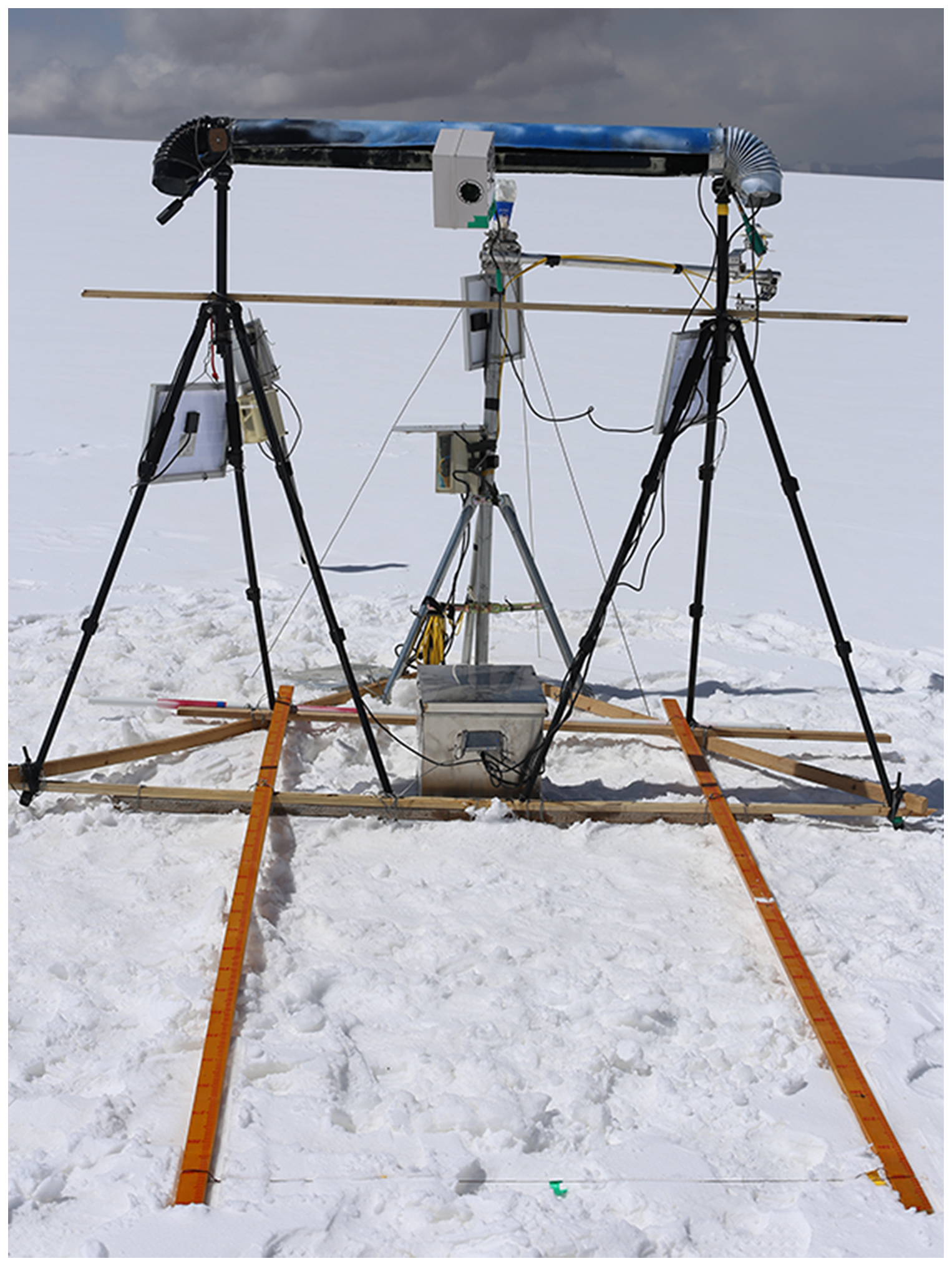
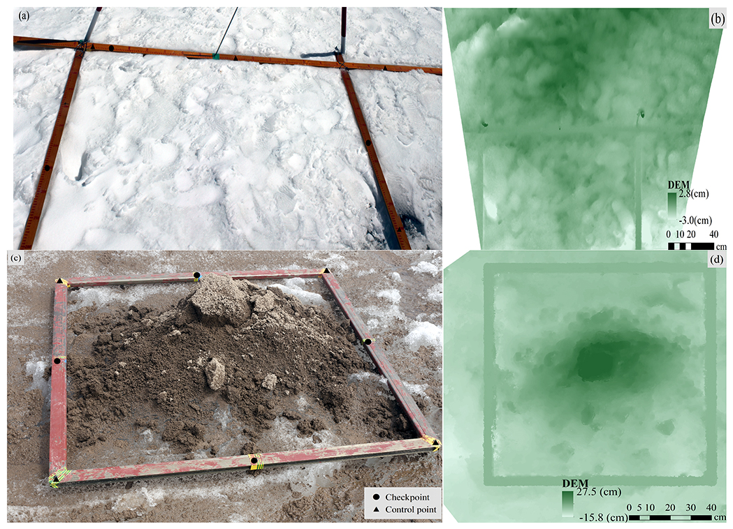
Figure 3Frames used for automatic and manual photogrammetry. (a) Wooden frame in situ set up for automatic photogrammetry; four control points and three checkpoints are shown on the frame. (b) Detrended DEM for the corresponding snow surface of (a). (c) Manual observation plot, with the four control points and four checkpoints shown on the aluminum frame. Ice surface hummock was covered with cryoconites. (d) Detrended DEM for the corresponding cryoconite surface of (c).
2.2 Automatic photogrammetry
The study began with the placement of an automatic close range photogrammetry measurement apparatus in the middle of the ice cap (4700 m; 39∘1.1′ N, 98∘53.4′ E; see Figs. 1b and 2). It was placed near the existing meteorological station. This was done on 10 July 2018. A wooden frame, 1.5 m wide and 2 m long, was put on the ice surface. This frame served as a geo-reference control field (Fig. 3a). Four feature points demarcated the control field; three additional points served as checkpoints. A Canon EOS 1300D cameras, with an image size of 5184×3456 pixels was connected to the frame. The camera lens was set in wide-angle mode (focal length of 27 mm). The f stop was fixed at f25 with an exposure time of 1∕320 s. The camera was programmed to automatically take seven pictures over a period of 10 min. The photography was repeated at 3 h intervals from 09:00 to 18:00, Beijing time. During the 10 min photography periods, the camera moved along a 1.5 m long slider rail. The camera was 1.7 m above the ice surface and moved along the control frame. The seven pictures taken during this period were merged to produce a picture of ice surface topography at millimeter scale (Fig. 3b). This apparatus took pictures over a period of 3 months (12 July to 15 September, the melting season). A total of 64 d of data were recorded. Each daily photography series produced four sets of pictures (12 h and 3 h intervals). The best-exposed photo sets were manually selected and used as that day's data. We also set up instrumentation to record incoming and reflected solar radiation. Samples were taken every 15 s; 10 min means were stored on a data logger (CR800, Campbell, USA) located at a height of 1.5 m. Surface elevation changes caused by accumulation and ablation were measured by a digital infrared hunting video camera, which took pictures of ice surface gauge stakes located near the automatic photogrammetry site.
2.3 Manual photogrammetry
Manual close-range photogrammetry was used to survey glacier surfaces at several different locations of the ice cap. Observations were made on 4 d: 12 and 25 July and 3 and 28 August. It should be noted that when the July measurements were performed, the ice cap surface was partially snow covered.
Channels account for only a small portion of the glacier surface area. These surfaces show extreme variability of z0 (Rippin et al., 2015; Smith et al., 2016). For that reason, we distributed the manual photogrammetry study sites over the glacier surface in such a way as to cover most surface types and topographic regions without including any channels (Fig. 1b). We photographed a total of 36 sites over the 4 d of observation.
Study plots were demarcated with a 1.1×1.1 m portable square aluminum frame. A geo-reference of the point cloud was enabled using control points established by eight cross-shaped screws on the aluminum frame (Fig. 3c). Photos (convergent photographs, low oblique photos in which camera axes converge toward one another) were taken at ∼ 1.6 m distances, covering an area of ∼ 1.75 m2. A total of 7 to 12 of such photos were taken at each survey site and surrounded the target area from different directions. The camera used was an EOS 6D 50 mm, with a fixed focal lens and an image size of 5472×3648 pixels. The f stop was fixed at f22 with an exposure time from 1∕25 to 1∕125 s.
2.4 Data processing
Structure-from-motion photogrammetry is revolutionizing the collection of detailed topographic data (Westoby et al., 2012; James et al., 2017). High-resolution DEMs produced from photographs acquired with consumer cameras need careful handling (James and Robson, 2014). In this study, both manual and automatically derived photographs were imported into a software program, Agisoft Photoscan Professional 1.4.0. This software allowed us to estimate camera intrinsic parameters, camera positions, and scene geometry. Agisoft Photoscan Professional is a commercial package, which implements all stages of photogrammetric processing (James et al., 2017). It has previously been used to generate three-dimensional point clouds and digital elevation models of debris-covered glaciers (Miles et al., 2017; Quincey et al., 2017; Steiner et al., 2018), ice surfaces and braided meltwater rivers (Javernick et al., 2014; Smith et al., 2016). In our study, we found that after new snowfall it was difficult to match feature points in the photo sets. A total of 3 d of automatic data could not be processed. We estimated z0 data for the missing days based on data from snowfall days at the automatic site.
2.5 Aerodynamic roughness estimation
Methods for measuring roughness at plot scale were first developed by soil scientists (Dong et al., 1992; Smith, 2014). Metrics such as the random roughness (RR) or root-mean-square height deviation (σ), the sum of the absolute slopes (ΣS), the microrelief index (MI) and the peak frequency (the number of elevation peaks per unit transect length) were used. Later these roughness indices were used to describe snow or ice surface roughness (Rees and Arnold, 2006; Fassnacht et al., 2009b; Irvine-Fynn et al., 2014).
Current photogrammetry methods produce high-resolution three-dimensional topographic data. Earlier two-dimensional profile-based methods for estimating surface roughness discard much of the potentially useful three-dimensional topographic data (Passalacqua et al., 2015). Smith et al. (2016) were able to use Eq. (1), developed by Lettau (1969), to make better use of the topographic data, using multiple point clouds and digital elevation models (DEMs). Fitzpatrick et al. (2019) also developed two methods for the remote estimation of z0 by utilizing lidar-derived DEM. In this method, z0 is quantified as follows:
where h* represents the effective obstacle height (m) and is calculated as the average vertical extent of micro-topographic variations, s is the silhouette area facing upwind (m2), S is the unit ground area occupied by micro-topographic obstacles (m2) and 0.5 is an averaged drag coefficient.
Based on the work of Lettau (1969), Munro (1989) simplified Eq. (1) by assuming that h* can equal twice the standard deviation of elevations in the de-trended profile, with the profile's mean elevation set to 0 m. The aerodynamic roughness length for a given profile then becomes
where f is the number of up-crossings above the mean elevation in profile, X is the length (m) of profile and σd is the standard derivation of elevations of profile. For manual photogrammetry, we put the aluminum frame horizontally over the ice surface, the plot is detrended by setting the control points at the z axis of the same values. For automatic photogrammetry, the control field of wooden frame was also laid horizontally over the ice surface, which lowered as the ice melted and maintained a horizontal position between the control field and ice surface. A DEM-based approach enables the roughness frontal area s to be calculated directly for each cardinal wind direction (Smith et al., 2016). The combined roughness frontal area was calculated across the plot, and the ground area occupied by micro-topographic obstacles is 1 m2. We used a DEM-based average () of the four cardinal wind directions to represent overall aerodynamic surface roughness. Based on the 30 min wind direction data at the August one ice cap, the daily upward wind direction DEM-based z0_DEM was also estimated at the automatic photogrammetry site. Considering that wind direction changed during the day, in this case we selected the prevailing wind direction to calculate frontal area s. The prevailing upwind direction DEM-based z0_DEM was applied to calculate turbulent heat flux. Using the Munro (1989) method, z0_profile was calculated for every profile (n=1000) in both orthogonal directions for each plot at the automatic photogrammetry site.
Table 2Control point RMSE for manual and automatic photogrammetry

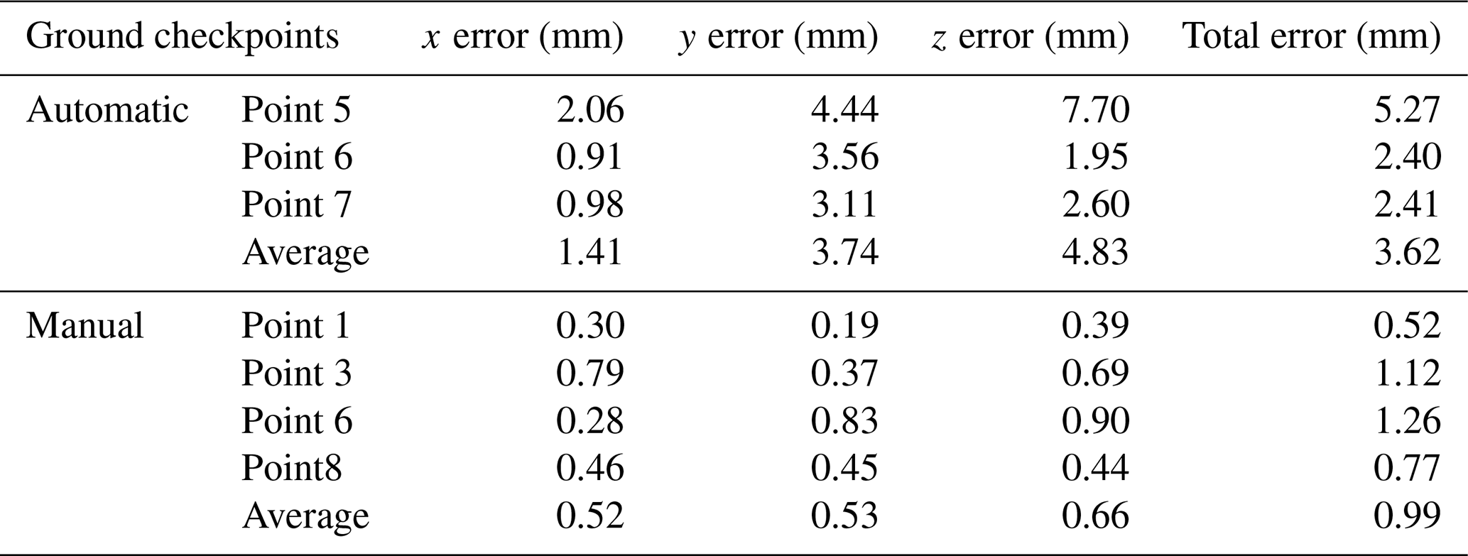
Table 3Checkpoint RMSE for manual and automatic photogrammetry.
2.6 Snow and ice surface energy balance calculation
The temporal variation in z0 at the automatic site was studied from energy balance perspective. The surface heat balance of a melting glacier is given by
where QM is the heat flux of melting, Qis is the incoming shortwave radiation, Qos is the outgoing shortwave radiation, QL is the net longwave radiation, QE is the latent heat flux; QH is the sensible heat flux, QP is the heat from rain and QG is subsurface heat flux.
In a horizontally homogeneous and steady surface state, the surface heat fluxes QE and QH can be calculated using either the bulk aerodynamic approach or profile method, based on the Monin–Obukhov similarity theory (e.g., Arck and Scherer, 2002; Garratt, 1992; Oke, 1987). In this study, 30 min observations at 4 m level and daily upward wind direction DEM-based z0 were used to calculate QE and QH based on the bulk method. The heat from rain is given by Konya and Matsumoto (2010):
where ρw is the density of water (1000 kg m−3), CW is the specific heat of water (4187.6 J kg−1 K−1), TW is the wet-bulb temperature (K) and Pr is the rainfall intensity (mm). The subsurface heat flux QG is estimated from the temperature–depth profile and is given by , where kT is the thermal conductivity, i.e., 0.4 Wm−1 K−1 for old snow and 2.2 W m−1 K−1 for pure ice (Oke, 1987).
In order to calculate Pr, we used the air temperatures recorded at the AWS. There is an elevation difference between the study site (4700 m) and the AWS (4790 m). Recorded air temperatures were corrected to account for the elevation difference. A lapse rate of −5.6 ∘C km−1 was applied based on observations made nearby (Chen et al., 2014). The ice cap is flat and open terrain so in this case wind speed and relative humidity at the study sites were assumed to be close to those observed at the AWS.

Figure 4Automatic and manual photogrammetry checkpoint errors. Panels (a), (c) and (e) are automatic photogrammetry standard deviation for the x, y and z axes, respectively. Panels (b), (d) and (f) are manual photogrammetry standard deviation for the x, y and z axes, respectively.

Figure 5(a) Variation in glacier surface aerodynamic roughness over time at the automatic observation site for the DEM-based and Munro (1989) profile-based approaches. Panel (b) shows a snow-covered surface on 13 July. Panel (c) shows a partially snow-covered surface on 23 July with cryoconite holes. Panels (d) and (e) show a smooth ice surface on 1 and 30 August. Panel (f) shows a rough ice surface on 13 September.
3.1 Photogrammetry precision
We used 17 plots to analyze the horizontal and vertical accuracy of our automatic photogrammetry and 31 plots for our manual photogrammetry. Based on the Agisoft Photoscan processing report, automatic photogrammetry average point density of the final plot point clouds was over 1 000 000 points m−2. DEMs of 1 mm resolution were generated at plot scale. The average geo-reference errors fluctuated at around 1 mm (see Tables 2 and 3). Total root-mean-square error (RMSE) of the automatic control points was 3.0±2.1 mm and for the checkpoints it was 3.62±1.6 mm. Vertical error for control points was 3.58 mm ± 3.01 mm and for the checkpoints it was 4.83 ± 2.9 mm (Tables 2 and 3). Standard deviation of control and checkpoint errors are all within 15 mm (Fig. 4a, c, e). Manually measured average point density of the final plot point clouds was > 6 000 000 points m−2. DEM of 1 mm resolution was generated at plot scale. The RMSE of four control points is 1.78±1.3 mm (Table 1). The control point vertical accuracy of manual photogrammetry is about 1.65±1.3 mm. The total RMSE of manual photogrammetry checkpoints is 0.99±0.3 mm and the vertical accuracy is 0.66±0.3 mm (see Tables 2 and 3). Standard deviation for the x, y and z axes were all within 5 mm (Fig. 4b, d, f).
Note that the control and checkpoint errors are larger for the automatic measurements than for the manual ones (see Fig. 4). We believe that this is the case because, rather than using static f stop and exposure times (as in automatic photogrammetry), researchers engaged in manual photogrammetry could adjust exposure time based on ice surface conditions. This allowed production of better quality photos even on cloudy or foggy days. This difference in survey design also caused more precise results for manual than automatic photogrammetry. For the automatic measurements, the camera was moving linearly and the density of tie points was much higher in the foreground compared to the background. For the manual method, photos were taken by surrounding the target area. This type of surface provided a much more robust elevation model and point density.
3.2 Aerodynamic surface roughness as measured by automatic photogrammetry
Data for ice surface roughness was collected by the automatic photogrammetry camera site from 12 July to 15 September, a period covering the whole melting season. Profile and DEM data show that z0 estimates vary by 2 orders of magnitude over the study period (Fig. 5). The upwind DEM-based data showed a z0_DEM varying from 0.1 to 1.99 mm (mean: 0.55 mm). The average of the four cardinal wind directions' DEM data shows a varying from 0.1 to 2.55 mm (mean: 0.57 mm). The average Munro profile-based z0_profile varied from 0.03 to 2.74 mm (mean 0.46 mm).
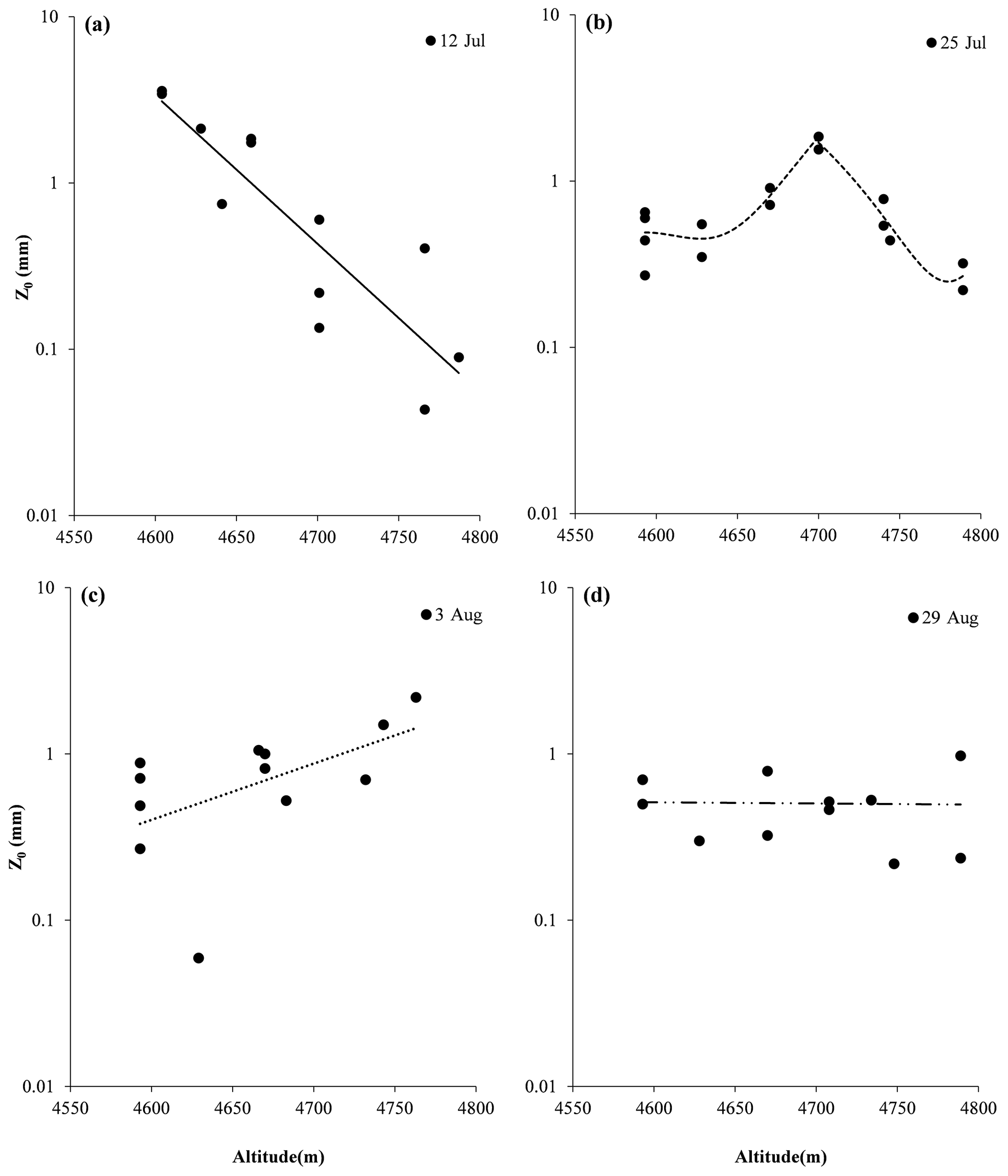
Figure 6Surface roughness vs. altitude, (a) as observed on 12 July, (b) 25 July, (c) 3 August and (d) 28 August.
At the start of the observation period of 12 July, snow covered the study site. As the snow melted, the ice cap surface z0 increased. During this period, z0 dropped to around 0.1 mm due to intermittent snowfall. On 21 July, cryoconites appeared on patches of snow crust, which led to patchy melt. From 21 to 24 July, overall increased from 0.1 to 1.6 mm. By 29 July, snow had disappeared from the study site, and z0 fluctuated but trended lower. From 29 July to 5 August bare ice covered the whole field of view; ranged from 0.18 to 0.56 mm. From 6 August to 3 September there was intermittent snowfall followed by melting, and ranged from 0.1 to 1.0 mm. From 4 to 14 September showed an overall increase, reaching a maximum of 2.55 mm on 8 September. There was intermittent snowfall during this period, which temporarily reduced , which then increased thanks to patchy microscale melting. After 14 September, snow covered the whole surface of the glacier and there was no melting and little fluctuation in z0.
It should be clear that either z0_profile or z0_DEM and varied following the same pattern during the melting season. There were two peaks in z0, both of which occurred in periods of transition: snow surface turning to ice around 24 July and ice surface turning to snow on 8 September. On 24 July and again on 8 and 13 September, glacier surfaces featured cryoconite holes and snow crust. Both the automatic and manual observations showed the same pattern: maximum z0 at the snow–ice transition belt during partially snow-covered periods.
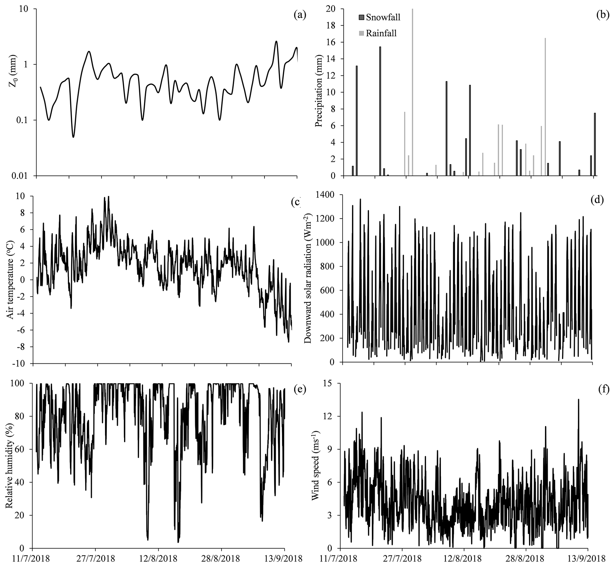
Figure 7Weather conditions at AWS over study period: (a) precipitation, (b) air temperature, (c) incident solar radiation, (d) relative humidity and (e) wind speed.
3.3 Surface roughness as measured by manual photogrammetry
No wind direction measurements were carried out during manual photogrammetry. In this case, we presented an average of the four cardinal directions to represent ice aerodynamic surface roughness. Analysis indicated that proved to have an interesting relationship with altitude. was highest in the transition zone between snow cover and ice. This zone moved up the ice cap during the melting season. On 12 July, ice surface roughness decreased from 3.2 to 0.25 mm as altitude increased (Fig. 6a; r=0.8429; ). Near the ice cap terminals at 4590 m, the ice surface featured porous snow and ice and many cryoconite holes. As altitude increased, the number of cryoconite holes decreased and snow coverage increased. At 4700 m the ice surface was predominantly snow covered and only a few small patches were free of snow. On 25 July, ice surface roughness fluctuated between 0.27 to 0.65 mm at the ice cap terminals (4593 m). At ∼ 4700 m, roughness increased to 1.85 mm. Above that point, roughness gradually decreased to 0.25 mm at the ice cap top, which was covered by snow (Fig. 6b).
On 3 August, the August one ice cap was predominantly bare ice and there was scattered snow crust at the ice cap top. The ice surface (terminal to top) showed a heavy deposit of cryoconite. Photogrammetric data collected manually revealed that ice surface roughness increased with altitude (Fig. 6c, r=0.7). From the terminals to the top of the ice cap, z0 varied from 0.06 to 2.2 mm. On 29 August, the ice cap surface roughness showed no significant correlation with altitude (Fig. 6d, ). varied from 0.2 to 0.98 mm (Fig. 6d). When we compare the results of the four surveys, we see that ice surface roughness was variable. Maximum z0 was seen at the snow and ice transition zone, where the ice surface featured both cryoconite holes and clean snow crust. Snow crust would have inhibited melting; cryoconite would have increased it. It is thus understandable that surface roughness would have been greater in such an area. Bare ice or snow cover both result in comparatively less roughness.
3.4 z0 and weather
Figure 7 compared and corresponding meteorological conditions of precipitation, air temperature, downward solar radiation, relative humidity and wind speed. Detailed analysis indicates snowfall was recorded from 12 to 24 July. In general, snowfall reduced roughness if it resulted in a fully snow-covered surface. However, if a patchy, shallow snow cover was formed, it tended to increase z0 after a short drop. For example, on 11 and 12 August, two successive sleety days created a patchy snow cover which soon increased z0. Between 26 July and 31 August there were 16 rainfall events, which tended to lower ice surface z0.
Daily temperatures during the study period ranged from −6.5 to 7.1 ∘C (mean: 1.3; Fig. 7c). It was 1.2 ∘C on 11 July. It increased to 3.6 ∘C on 24 July (the date when z0 was highest). It continued increasing until 29 July, when it reached its highest annual of 7.1 ∘C. During this period z0 continuously declined. From 28 July to the end of August temperatures fluctuated between −0.3 and 5.7 ∘C with no evident trend. also fluctuated slightly, showing no obvious trend. In September air temperature quickly dropped from 0.6 to −6.5 ∘C. There were large fluctuations in z0 during this period. The largest fluctuations appeared when air temperatures dropped from positive to negative.
Daily downward mean solar radiation fluctuated dramatically during the study period due to cloudy and overcast conditions (Fig. 7d). Incident solar radiation fluctuated between 129 and 753 W m−2 (mean: 469 W m−2). From 29 July to the end of August, the weather was cloudy, warm, calm, and humid most of the time (Fig. 7b, c, e, f) and was relatively stable, except when there was intermittent snowfall-induced fluctuation. After September, the weather again became cold and dry and z0 was quite variable.
3.5 Ice surface energy balance at automatic z0 observation study site
The following section analyzes the changes in surface energy balance at the automatic site. Meteorological observation records allowed us to study the factors that control ice surface roughness. Net radiation varied from −9.7 to 260.2 W m−2 (mean: 95.3 W m−2) during the study period. This constituted the largest energy flux affecting glacier surface energy balance. It accounted for 84 % of total incoming flux (Fig. 8). Net radiation was relatively low in the first 13 d of the study period (mean: 69.3 W m−2), when the glacier surface was covered with snow. In the succeeding 5 d, net radiation increased to 103.9 W m−2. At this time the ice surface exhibited a patchwork of snow, ice, and cryoconite. From 29 July to 5 August the surface of the study site was composed of ice with a dusting of cryoconite. Net radiation reached a height of 183 W m−2. There was intermittent snowfall from 6 August to 8 September. Net radiation dropped to a mean 93 W m−2. Snow cover then appeared and net radiation dropped to a low of 46 W m−2.
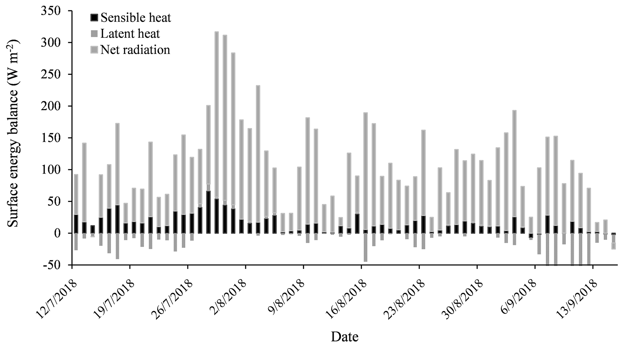
Figure 8Daily mean energy balance at the middle of the glacier study site, which was close to the automatic photogrammetry site.
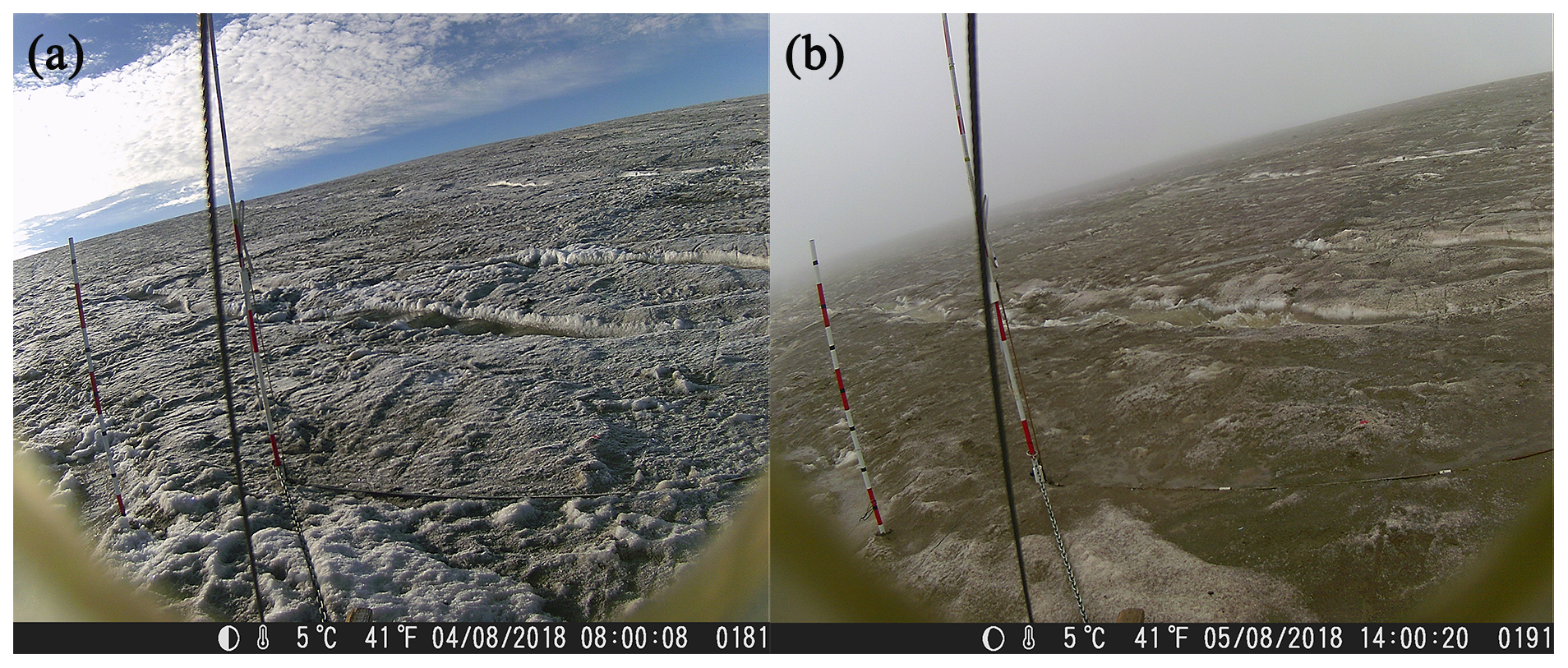
Figure 9Ice surface overview at the automatic photogrammetry site before and after a strong rainfall event captured by an automatic digital infrared hunting video camera: (a) photograph taken before the rainfall event on 4 August of 2018 and (b) photograph taken after the strong rainfall event on 5 August of 2018.

Figure 10Comparison of observed daily mass balance and modeled daily mass balance. Mass balance measurements were taken from 12 July to 29 August. Measurements of surface lowering were converted into water equivalents using density values.
Bulk-method-estimated results indicate that sensible heat (QH) was the second largest energy flux component of in surface energy balance during the study period (Fig. 8). The sensible heat daily mean varied from −7.1 to 66.3 W m−2. It accounted for −28 % to 32 % (mean: 15 %) of the net energy flux. Latent heat was generally small throughout the study period. Daily mean of latent heat varied from −80.1 to 11.1 W m−2 (mean: −13.2 W m−2). It accounts for a mere 0.9 % for the total incoming flux. It was negative from 11 to 26 July when the ice surface was snow covered. After 26 July the latent heat was mainly positive in the following 10 d (the ice surface was pure ice or partially snow covered). From 6 August to the end of the study period (15 September) it was predominantly negative.
From 25 July to 5 August rainfall energy varied from 0 to 11.7 W m−2 (mean: 0.3 W m−2). Rainfall accounted for a mere 0.2 % of total incoming flux. One event accounted for much of the total: on 28 July a 31 mm rainfall event added a flux of 11.7 W m−2, which resulted in visible smoothing of the ice surface (Fig. 9). Compared to other energy components, QG was very small, with a daily mean of −0.65 W m−2 and a maximum and minimum of −0.4 and −2.1 W m−2, respectively.
3.6 Modeled vs. observed surface ablation
Based on the previously listed measurements of energy fluxes, we calculated the probable surface ablation at the automatic photogrammetry site. We took into account observed net radiation, bulk-method-calculated turbulent heat fluxes, heat from rainfall and subsurface heat flux. There was good agreement between the model and observed results (Fig. 10).
Figure 11 shows the relationship between estimated daily upward wind direction DEM-based z0_DEM and the main energy flows. Scatter diagrams showed a positive relationship between z0_DEM and net shortwave radiation (Fig. 11a, r=0.1) and a significant negative relationship between z0_DEM and net longwave radiation (Fig. 11b, ), Graphing z0_DEM vs. bulk-method-estimated latent heat showed a significant negative exponential relationship (Fig. 11d, ). The scatter diagram showed no significant relationship between z0_DEM and the bulk-method-estimated sensible heat (Fig. 11c). The average of the Munro profile-based z0_profile, DEM-based and the main energy items are also analyzed. Scatter diagrams showed a significant negative relationship between z0_profile and net longwave radiation (Fig. S1a, ). Graphing z0_profile vs. the bulk-method-estimated latent heat showed a significant negative exponential relationship (Fig. S1d, ). The scatter diagram showed no significant relationship between z0_profile and the bulk-method-estimated sensible heat (Fig. S1c). vs. the bulk-method-estimated latent heat showed a significant negative exponential relationship (Fig. S2d, ). In the scatter diagrams between and net shortwave radiation, the bulk-method-estimated sensible heat showed no significant relationship.
Because net shortwave radiation and turbulent heat fluxes were the main energy fluxes affecting ice surface roughness, we calculated a turbulent heat proportion index:
Note that aerodynamic surface roughness on days when snow fell was strongly affected by the amount of the snowfall. If we exclude snowfall days and snow-covered period, we see a significant exponential relationship between ice surface z0_DEM and LS (Fig. 12a, ). The scatter diagrams showed a significant exponential relationship between ice surface z0_profile and LS and net longwave radiation (Fig. 12c, ). vs. LS also showed a significant exponential relationship (Fig. 12b, ). Scatter diagrams in Fig. 12 also showed z0 did not keep decreasing when LS was above 0.2. z0_DEM, z0_profile and were around 0.56±0.21, 0.33±0.03 and 0.6±0.26 mm, respectively.
Table 4The lagged correlation between z0 and the main energy items during the melting season; the sensible heat and latent heat were calculated here based on the bulk method.

n= the number of samples, .
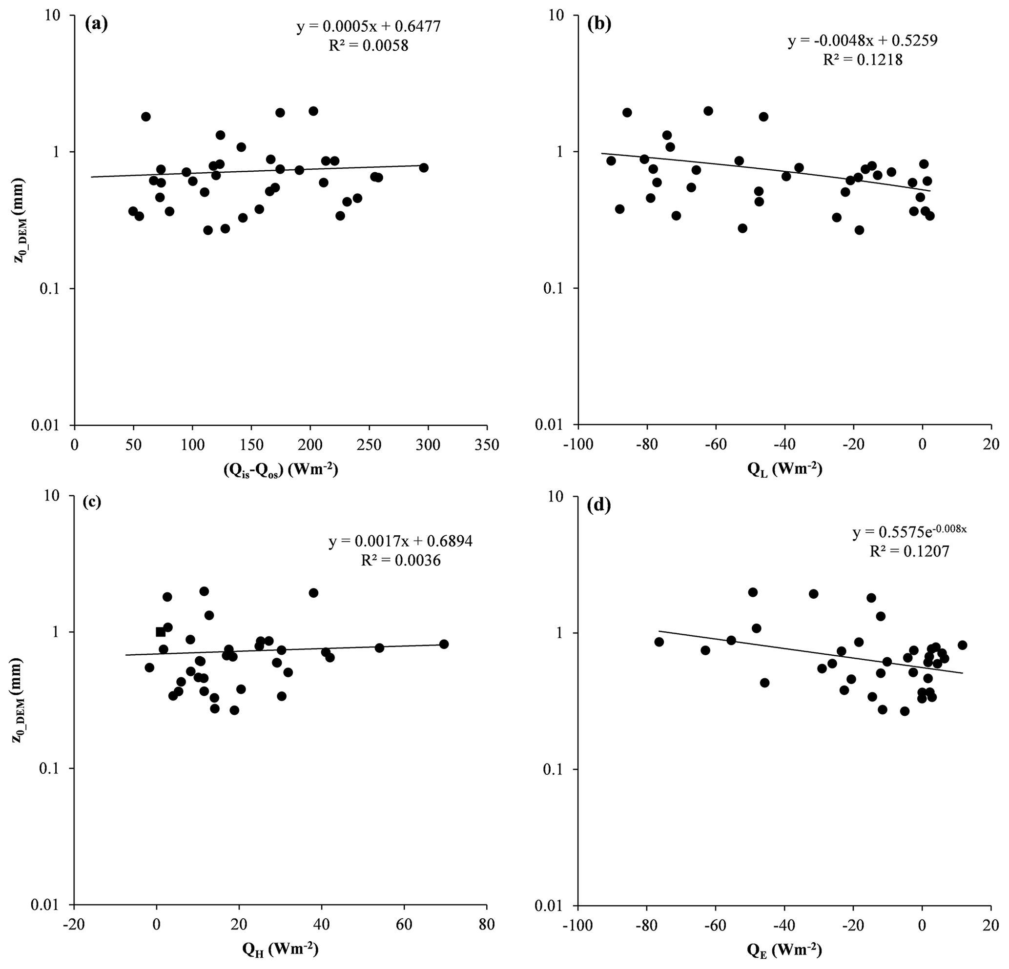
Figure 11Daily upward wind direction of DEM-based z0_DEM vs. energy inputs: (a) z0_DEM vs. net shortwave radiation, (b) z0_DEM vs. net longwave radiation, (c) z0_DEM vs. bulk-method-calculated sensible heat and (d) z0_DEM vs. bulk-method-calculated latent heat.
The z0 (z0_DEM and ) vs. LS graph indicates that when turbulence and rainfall heat increased, aerodynamic surface roughness decreased. As soon as LS is above 0.2, the ice surface will not keep smoothing and z0 sustains its lowest stage. Time series correlation of all main energy items and z0_profile were performed. Table 4 shows an example of the lagged correlations between z0_profile and five variables. The z0 and net shortwave radiation displayed a positive correlation with 0 to 1 d lag time. The z0 response to QE with a correlation of −0.6 showed a lag of 0 to 1 d. The z0_profile also had a negative relationship with QL with no lag or 1 d lag time. The z0_profile response to LS with a correlation of −0.58 was with a lag of 0 to 2 d. A total of 0 to 2 d lag time gives an indication of the effort limitations of the main energy items over ice surface z0. In other words, a sunny and cold day facilitates rough ice surfaces and warm and cloudy days tend to produce a smoother ice surface. When net shortwave radiation is higher and latent and sensible heat are smaller, z0 tends to be higher for the next 2 d. When net shortwave radiation is smaller, as on cloudy days, any snowfall or rainfall is usually associated with smaller z0 for the following 2 d. Under a negative QM, the surface z0 would not be affected by melting process.
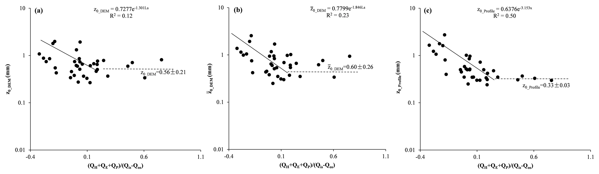
Figure 12Aerodynamic surface roughness vs. LS. Where ), in (a) z0_DEM was estimated based on DEM-based prevailing upwind direction, in (b) was the average of the four cardinal wind directions' z0 in order to represent overall aerodynamic surface roughness and in (c) z0_profile was the average of two orthogonal directions z0.
4.1 Automatic and manual photogrammetric methods
Photogrammetric techniques such as Structure from Motion (SfM) (James and Robson, 2012) and Multi-view Stereo (MVS) represent low-cost options for acquiring high-resolution topographic data. Such approaches require relatively little training and are extremely inexpensive (Westoby et al., 2012; Fonstad et al., 2013; Passalacqua et al., 2015). We used both automatic and manual photogrammetric methods to sample spatial and temporal z0 variation at the August one ice cap. Adjustments to exposure time based on ice surface conditions and survey design of the area surrounding the target made the manual photogrammetry more precise than automatic photogrammetry (Tables 2 and 3). However, precision is not always the major concern. The glacier surface was a harsh (even punishing) environment for the researchers doing manual photogrammetry. In addition, manual photogrammetry took much longer. Automatic methods reduced hours of field work, spared researchers and produced nearly continuous data. Cloudy or frosty weather affected automatic photogrammetry exposures, and heavy snowfalls resulted in a textureless surface. Nevertheless, it is likely that photogrammetry techniques will continue to improve and that these drawbacks may be mitigated.
4.2 Spatial and temporal variability of z0
Previous studies of glacier surfaces roughness have rarely covered the whole glacier, from the terminals to the top of the ice cap, in one melting season (Föhn, 1973; Smeets et al., 1999; Denby and Smeets, 2000; Greuell and Smeets, 2001; Albert and Hawley, 2002; Brock et al., 2006; Smeets and Van den Broeke, 2008; Smith et al., 2016). This whole-glacier study allowed us to follow the movement of the transition zone, where snow was melting and exposing ice, from the terminals to the top of the ice cap. The transition zone moved up as the melting season proceeded, thus roughening the surface of the glacier and raising z0. At the start of the melting season, snow cover first disappeared, leaving an ice surface at the terminal end of the August one ice cap, i.e., at the lower altitude. This newly exposed surface was rougher (z0 was higher) than on the upper part of glacier, which was still snow covered (see the black line in Fig. 6a for z0 distribution at different altitudes). As the snowline shifted to higher altitudes, ice surface increased, as did z0 (see the dashed black curve in Fig. 6b). As the melting continued, the snow and ice transition belt reached the top of glacier (see the dotted curve in Figure 6c). When the ice cap was completely free of snow, z0 and elevation were no longer correlated (see the dotted–dashed line in Fig. 6d). In summary, maximum z0 was recorded at the cross-glacier transition zone between snow and ice. This zone shifted from lower altitude to higher altitude, from the terminals to the top of the ice cap, during the melting season. The spatial pattern of z0 distribution affected turbulent fluxes. The transition zone had maximum z0, and the zone also migrated across much of the glacier, highlighting the importance of transient surface characteristics.
Micro-topography, wind profile and eddy covariance methods generate a wide range of z0 values for snow and ice surfaces (Grainger and Lister, 1966; Munro, 1989; Bintanja and Broeke, 1995; Schneider, 1999; Hock and Holmgren, 2005; Brock et al., 2006; Andreas et al., 2010; Gromke et al., 2011). In this study, z0_profile, z0_DEM and showed similar variation pattern during the melting season. The difference of z0_profile, z0_DEM, and were within 1 order of magnitude. The latent and sensible heat calculated by z0_profile, z0_DEM and were highly relevant among these methods. The automatic photogrammetry estimated z0 for snow-covered surfaces ranged from 0.1 to 0.55. New snowfall at the snow surface in July formed the lowest z0 values. Previous studies have shown that freshly fallen snow is subject to rapid destructive metamorphism (McClung and Schaerer, 2006), which can dramatically change the roughness of fresh snow surfaces (Fassnacht et al., 2009b). Our study showed that z0 followed an increasing trend during the melting season. Intermittent snowfall first decreased snow surface z0, which then began to increase as the snow surface deteriorated. In the data from Clifton et al. (2008), snow surface z0 was estimated at between 0.17 to 0.6 mm in a wind tunnel experiment. In an analysis of ultrasonic anemometer recorder data over snow-covered sea ice, Andreas et al. (2010) found z0 values ranging from 10−2 to 101 mm. In a wind tunnel experiment of fresh snow with no-drift conditions, Gromke et al. (2011) estimated z0 to be between 0.17 to 0.33 mm, with no apparent dependency on the friction velocity. Our snow surface data showed that z0 values fluctuated between 0.03 to 0.55 mm, consistent with some of those wind tunnel studies. The scatter of z0 data reported in some studies is quite large, with a range of 10−2 to 101 mm. The result may be attributed to the occurrence of snow drift, a transitional rough-flow regime and large uncertainties in the estimation of friction velocities that propagate to the computation of z0 (Andreas et al., 2010; Gromke et al., 2011). In contrast, the small scatter in our data was induced only by the natural variability of snow surface roughness.
For patchy snow-covered ice surfaces, z0 varied from 0.5 to 2.6 mm and ice surface z0 varied from 0.24 to 1.1 mm. During the melting season, there were no blowing snow events and snow surface z0 was relatively smaller than in patchy snow-covered surface or ice surface. Ice surface z0 was generally larger than snow surface and smaller than patch snow-covered surface. Our results match values reported in studies reporting results ranging from 0.1 to 6.9 mm in Qilian mountain glaciers (Guo et al., 2018; Sun et al., 2018). Our results showed that z0 reached its maximum at the end of the summer melt, which matched wind profile measurements by Smeets and Broeke (2008).
The aerodynamic surface roughness is influenced by both the boundary layer and the surface. In this study, the micro-topographic estimated aerodynamic surface roughness only considers surface topography at plot scale but its variability is influenced by its surrounding topography and the boundary layer. Thus, the results of z0 estimated in this study still need to be validated by wind tower or eddy covariance observations. However, micro-topographic roughness metrics are a very strong proxy for z0 (e.g., Nield et al., 2013), so we have much more confidence in the temporal and spatial variability presented by this work.
4.3 Effects of surface energy balance components on aerodynamic surface roughness
Aerodynamic roughness is associated with the geometry of ice roughness elements (Kuipers, 1957; Lettau, 1969; Munro, 1989). Surface geometry roughness develops due to local melt inhomogeneities in melting season. In earlier works, researchers argued that a variety of ablation forms, such as sun cups, penitents, cryoconite holes or dirt cones, are formed by the sun (Matthes, 1934; Lliboutry, 1954; McIntyre, 1984; Rhodes et al., 1987; Betterton, 2000). These ablation forms develop in regions with bright sunlight and cold, dry weather conditions are apparently required (Rhodes et al., 1987). These structures are observed to decay if the weather is cloudy or very windy (Matthes, 1934; Lliboutry, 1954; McIntyre, 1984).
The August one ice cap dust concentrations are high in the melting season. Cryoconites are unevenly distributed over the ice surface, leading to differential absorption of shortwave radiation at microscale. This process results in the roughening of the ice surface, a process that enhances turbulent heat exchange across the atmospheric boundary layer–ice interface. When the air temperature is above 0 ∘C, the ice surface keeps melting. The turbulent heat smooths the ice surface, increases the cryoconite concentration over the ice surface and decreases ice surface albedo, enhancing shortwave radiation absorption (Fig. 9). This roughening and smoothing process makes ice surface z0 fluctuate at around 0.56 mm as long as the air temperature is above 0 ∘C. When the temperature drops below 0 ∘C, bright sunlight and dry weather shutdown the ice surface smoothing process. The shortwave radiation induces even rougher ice and larger z0 until snow covers the ice surface. At the August one ice cap, the turbulent heat contributes a small portion of incoming energy, but the smoothing ice surface process decreases ice surface albedo and seems to enhance ice surface shortwave radiation. The z0 fluctuation in the melt season is similar, with cryoconite holes developing when the radiative flux is dominant and decaying when turbulent heat is dominant (McIntyre, 1984; Takeuchi et al., 2018). The glacier surface energy balance components vs. z0 analysis in this study confirm that the main energy items of net shortwave radiation and turbulent heat flux affect the same-day z0 and following 2 d of z0. This study found an exponential relationship between z0 and LS. The delicate role of z0 played in the ice surface balance is still not fully known. Further comparative studies are needed to investigate the z0 variation through eddy covariance and profiling methods and DEM-based z0 estimation.
Manual and automatic measurements of snow and ice surface roughness at the August one ice cap showed spatial and temporal variation in z0 over the melting season. Manual measurements, taken from the terminals to the top of the ice cap, show that the nature of the surface cover features are correlated with z0 rank in the following order: transition region > pure ice area or pure snow area. The transition region forms a zone of maximum z0, which shifts over the melting season from the terminals to the top of the ice cap. The observed z0 vs. energy items analysis indicated that LS (turbulent heat index) was also an important determinant of ice aerodynamic surface roughness.
Aerodynamic surface roughness is a major parameter in calculations of glacier surface turbulent heat fluxes. In previous studies investigators used a constant z0 value for the whole surface of the glacier. This study captures a much smaller-scale variation in spatial and temporal glacier surface aerodynamic roughness through automatic and manual photogrammetric observations. Such close observation of variation in z0 certainly enhanced the accuracy of the surface energy balance models developed in the course of this study.
This study was carried out at an ice cap with a neat ordering of its annual layers. The August one ice cap moved slowly, no crevasses were formed over the ice cap and channels were not considered in this study. In this case, a more moderate variation in z0 was estimated than would be found for debris-covered glaciers (Miles et al., 2017; Quincey et al., 2017). Uneven or heterogeneous ice surfaces such as sastrugi, crevasses, channels and penitents could greatly affect ice surface aerodynamic surface roughness, and it would be hard to estimate its z0 based on a profile method. SfM estimation of z0 might be a good choice at a macroscale. In the accumulation season, more attention would need to be paid to spatial and temporal variations in z0, as z0 is a key parameter for sublimation calculation during this period. Studies have indicated that the Lettau (1969) approach calculated z0 dependent on plot scale and resolution. In this study, we only select 1 m×1 m scale at 1 mm resolution to study spatial and temporal variability. Further comparative studies of z0 are needed at different scales and resolutions.
All of the observation and model input and output data presented in this study are available upon request to the corresponding author (Rensheng Chen, crs2008@lzb.ac.cn).
JL and RC designed the study and wrote the paper. JL and CH carried out field-based manual photogrammetry observations.
The authors declare that they have no conflict of interest.
We thank the editor and the two reviewers for their insightful comments and ideas that improved the paper.
This research has been supported by the National Natural Science Foundation of China (grant nos. 41877163 and 41671029).
This paper was edited by Valentina Radic and reviewed by Joshua Chambers and Evan Miles.
Albert, M. R. and Hawley, R. L.: Seasonal changes in snow surface roughness characteristics at Summit, Greenland: implications for snow and firn ventilation, Ann. Glaciol., 35, 510–514, doi:10.3189/172756402781816591, 2002.
Andreas, E. L.: Parameterizing scalar transfer over snow and ice: A review, J. Hydrometeorol., 3, 417–432, 2002.
Andreas, E. L., Persson, P. O. G., Jordan, R. E., Horst, T. W., Guest, P. S., Grachev, A. A., and Fairall, C. W.: Parameterizing turbulent exchange over sea ice in winter, J. Hydrometeorol., 11, 87–104, doi:10.1175/2009JHM1102.1, 2010.
Arck, M., and Scherer, D.: Problems in the determination of sensible heat flux over snow, Geogr. Ann., 84, 157–169, doi:10.1111/1468-0459.00170, 2002.
Betterton, M. D.: Formation of structure in snowfields: Penitentes, suncups, and dirt cones, Phys. Rev. E, 63, 056129, doi:10.1103/PhysRevE.63.056129, 2000.
Bintanja, R. and Van den Broeke, M.: Momentum and scalar transfer-coefficients over aerodynamically smooth Antarctic surfaces, Bound.-Lay. Meteorol., 74, 89–111, doi:10.1007/BF00715712, 1995.
Brock, B. W., Willis, I. C., and Sharp, M. J.: Measurement and parameterization of aerodynamic roughness length variations at Haut Glacier d'Arolla, Switzerland, J. Glaciol., 52, 1–17, 2006.
Chen, R. S., Song, Y. X., Kang, E. S., Han, C. T., Liu, J. F., Yang, Y., Qing, W. W., and Liu, Z. W.: A Cryosphere-Hydrology Observation System in a Small Alpine Watershed in the Qilian Mountains of China and Its Meteorological Gradient, Arct. Antarct. Alp. Res., 46, 505–523, doi:10.1657/1938-4262-46.2.505, 2014.
Clifton, A., Manes, C., Rueedi, J. D., Guala, M., and Lehning, M.: On shear-driven ventilation of snow, Bound.-Lay. Meteorol., 126, 249–261, doi:10.1007/s10546-007-9235-0, 2008.
Denby, B. and Smeets, C.: Derivation of turbulent flux profiles and roughness lengths from katabatic flow dynamics, J. Appl. Meteorol., 39, 1601–1612, 2000.
Denby, B. and Snellen, H.: A comparison of surface renewal theory with the observed roughness length for temperature on a melting glacier surface, Bound.-Lay. Meteorol., 103, 459–468, 2002.
Dong, W. P., Sullivan, P. J., and Stout, K. J.: Comprehensive study of parameters for characterizing three-dimensional surface topography I: Some inherent properties of parameter variation, Wear, 159, 161–171, 1992.
Fassnacht, S. R., Stednick, J. D., Deems, J. S., and Corrao, M. V.: Metrics for assessing snow surface roughness from digital imagery, Water Resour. Res., 45, W00D31, doi:10.1029/2008wr006986, 2009a.
Fassnacht, S. R., Williams, M., and Corrao, M.: Changes in the surface roughness of snow from millimetre to metre scales, Ecol. Complex., 6, 221–229, doi:10.1016/j.ecocom.2009.05.003, 2009b.
Fitzpatrick, N., Radić, V., and Menounos, B.: A multi-season investigation of glacier surface roughness lengths through in situ and remote observation, The Cryosphere, 13, 1051–1071, https://doi.org/10.5194/tc-13-1051-2019, 2019.
Föhn, P. M. B.: Short-term snow melt and ablation derived from heat-and mass-balance measurements, J. Glaciol., 12, 275–289, 1973.
Fonstad, M. A., Dietrich, J. T., Courville, B. C., Jensen, J. L., and Carbonneau, P. E.: Topographic structure from motion: a new development in photogrammetric measurement, Earth Surf. Proc. Land., 38, 421–430, doi:10.1002/esp.3366, 2013.
Garratt, J. R.: The Atmospheric Boundary Layer, Cambridge University Press, New York, 1992.
Grainger, M. and Lister, H.: Wind speed, stability and eddy viscosity over melting ice surfaces, J. Glaciol., 6, 101–127, 1966.
Greuell, W. and Smeets, P.: Variations with elevation in the surface energy balance on the Pasterze (Austria), J. Geophys. Res.-Atmos., 106, 31717–31727, 2001.
Gromke, C., Manes, C., Walter B, Lehning, M., and Guala, M.: Aerodynamic roughness length of Fresh snow, Bound.-Lay. Meteorol., 141, 21–34, doi:10.1007/s10546-011-9623-3, 2011.
Guo, S. H., Chen, R. S., Liu, G. H., Han, C. T., Song, Y. X., Liu, J. F., Yang, Y., Liu, Z. W., Wang, X. Q., and Liu, X. J.: Simple Parameterization of Aerodynamic Roughness Lengths and the Turbulent Heat Fluxes at the Top of Midlatitude August-One Glacier, Qilian Mountains, China, J. Geophys. Res.-Atmos., 123, 12066–12080, doi:10.1029/2018JD028875, 2018.
Guo, W., Liu, S., Xu, J., Wu, L., Shangguan, D., Yao, X., Wei, J., Bao, W., Yu, P., Liu, Q., and Jiang, Z.: The second Chinese glacier inventory: data, methods and results. J. Glaciol., 61, 357–372, doi:10.3189/2015jog14j209, 2015.
Hock, R. and Holmgren, B.: A distributed surface energy-balance model for complex topography and its application to Storglaciären, Sweden, J. Glaciol., 51, 25–36, doi:10.3189/172756505781829566, 2005.
Irvine-Fynn, T., Sanz-Ablanedo, E., Rutter, N., Smith, M., and Chandler, J.: Measuring glacier surface roughness using plot-scale, close-range digital photogrammetry, J. Glaciol., 60, 957–969, doi:10.3189/2014JoG14J032, 2014.
James, M. R. and Robson, S.: Mitigating systematic error in topographic models derived from UAV and ground-based image networks, Earth Surf. Proc. Land., 39, 1413–1420, doi:10.1002/esp.3609, 2014.
James, M. R., Robson, S., and Smith, M. W.: 3-D uncertainty-based topographic change detection with structure-from-motion photogrammetry: precision maps for ground control and directly georeferenced surveys, Earth Surf. Proc. Land., 42, 1769–1788, doi:10.1002/esp.4125, 2017.
James, M. and Robson, S.: Straightforward reconstruction of 3D surfaces and topography with a camera: Accuracy and geoscience application, J. Geophys. Res.-Earth, 117, F03017, doi:10.1029/2011JF002289, 2012.
Javernick, L., Brasington, J., and Caruso, B.: Modeling the topography of shallow braided rivers using Structure-from-Motion photogrammetry, Geomorphology, 213, 166–182, doi:10.1016/j.geomorph.2014.10.006, 2014.
Konya, K. and Matsumoto, T.: Influence of weather conditions and spatial variability on glacier surface melt in Chilean Patagonia, Theor. Appl. Climatol., 102, 139–149, 2010.
Kuipers, H.: A relief meter for soil cultivation studies, Neth. J. Agr. Sci., 5, 255–262, 1957.
Lacroix, P., Legrésy, B., Coleman, R., Dechambre, M., and Rémy, F.: Dual-frequency altimeter signal from Envisat on the Amery ice-shelf, Remote Sens. Environ., 109, 285–294, doi:10.1016/j.rse.2007.01.007, 2007.
Lacroix, P., Legrésy, B., Langley, K., Hamran, S., Kohler, J., Roques, S., Rémy, F., and Dechambre, M.: In situ measurements of snow surface roughness using a laser profiler, J. Glaciol., 54, 753–762, doi:10.3189/002214308786570863, 2008.
Lehning, M., Bartelt, P., Brown, B., and Fierz, C.: A physical SNOWPACK model for the Swiss avalanche warning: Part III: meteorological forcing, thin layer formation and evaluation, Cold Reg. Sci. Technol., 35, 169–184, doi:10.1016/S0165-232X(02)00072-1, 2002.
Lettau, H.: Note on aerodynamic roughness parameter estimation the basis of roughness element description, J. Appl. Meteorol., 8, 828–832, 1969.
Lliboutry, L.: The origin of penitents, J. Glaciol., 2, 331–338, https://doi.org/10.3189/S0022143000025181, 1954.
Manninen, T., Anttila, K., Karjalainen, T., and Lahtinen, P.: Automatic snow surface roughness estimation using digital photos, J. Glaciol., 58, 993–1007, doi:10.3189/2012JoG11J144, 2012.
Matthes F. E.: Ablation of snow-fields at high altitudes by radiant solar heat, T. AGU, 15, 380–385, 1934.
McClung, D. and Schaerer, P. A.: The avalanche handbook, The Mountaineers Books, Seattle, WA, 2006.
McIntyre, N. F.: Cryoconite hole thermodynamics, Can. J. Earth Sci., 21, 152–156, 1984.
Miles, E. S., Steiner, J. F., and Brun, F.: Highly variable aerodynamic roughness length (z0) for a hummocky debris-covered glacier, J. Geophys. Res.-Atmos., 122, 8447–8466, doi:10.1002/2017JD026510, 2017.
Munro, D. S.: Surface roughness and bulk heat transfer on a glacier: comparison with eddy correlation, J. Glaciol., 35, 343–348, doi:10.3189/S0022143000009266, 1989.
Nield, J. M., King, J., Wiggs G. F. S., Leyland, J., Bryant, R. G., Chiverrell, R. C., Darby, S. E., Eckardt, F. D., Thomas, D. S. G., Vircavs, L. H., and Washington, R.: Estimating aerodynamic roughness over complex surface terrain, J. Geophys. Res.-Atmos., 118, 12948–12961, doi:10.1002/2013JD020632, 2013.
Oke, T. R.: Boundary layer climates, Routledge, London, 1987.
Oveisgharan, S. and Zebker, H. A.: Estimating snow accumulation from InSAR correlation observations, IEEE T. Geosci. Remote, 45, 10–20, doi:10.1109/TGRS.2006.886196, 2007.
Passalacqua, P., Belmont, P., Staley, D. M., Simley, J. D., Arrowsmith, J. R., Bode, C. A., Crosby, C., DeLong, S. B., Glenn, N. F., Kelly, S. A., Lague, D., Sangireddy, H., Schaffrath, K., Tarboton, D., Wasklewicz, T., and Wheaton, J. M.: Analyzing high resolution topography for advancing the understanding of mass and energy transfer through landscapes: A review, Earth-Sci. Rev., 148, 174–193, doi:10.1016/j.earscirev.2015.05.012, 2015.
Qing, W., Han, C. T., and Liu, J.: Surface energy balance of Bayi Ice Cap in the middle of Qilian Mountains, China, J. Mt. Sci., 15, 1229–1240, https://doi.org/10.1007/s11629-017-4654-y, 2018
Quincey, D., Smith, M., Rounce, D., Ross, A., King, O., and Watson, C.: Evaluating morphological estimates of the aerodynamic roughness of debris covered glacier ice, Earth Surf. Proc. Land., 42, 2541–2553, doi:10.1002/esp.4198, 2017.
Rees, W. G.: A rapid method of measuring snow-surface profiles, J. Glaciol., 44, 674–675, doi:10.3189/S0022143000002197, 1998.
Rees, W. G. and Arnold, N. S.: Scale-dependent roughness of a glacier surface: implications for radar backscatter and aerodynamic roughness modelling, J. Glaciol., 52, 214–222, doi:10.3189/172756506781828665, 2006.
Rhodes, J. J., Armstrong, R. L., and Warren, S. G.: Mode of formation of “ablation hollows” controlled by dirt content of snow, J. Glaciol., 33, 135–139, 1987.
Rippin, D. M., Pomfret, A., and King, N.: High resolution mapping of supra-glacial drainage pathways reveals link between micro-channel drainage density, surface roughness and surface reflectance, Earth Surf. Proc. Land., 40, 1279–1290, doi:10.1002/esp.3719, 2015.
Rounce, D. R., Quincey, D. J., and McKinney, D. C.: Debris-covered glacier energy balance model for Imja–Lhotse Shar Glacier in the Everest region of Nepal, The Cryosphere, 9, 2295–2310, https://doi.org/10.5194/tc-9-2295-2015, 2015.
Schneider, C.: Energy balance estimates during the summer season of glaciers of the Antarctic Peninsula, Global Planet. Change, 22, 117–130, doi:10.1016/S0921-8181(99)00030-2, 1999.
Smeets, C. J. P. P., and Van den Broeke, M. R.: Temporal and spatial variations of the aerodynamic roughness length in the ablation zone of the Greenland ice sheet, Bound.-Lay. Meteorol., 128, 315–338, doi:10.1007/s10546-008-9291-0, 2008.
Smeets, C. J. P. P., Duynkerke, P. G., and Vugts, H. F.: Turbulence characteristics of the stable boundary layer over a mid-latitude glacier. Part II: Pure katabatic forcing conditions, Bound.-Lay. Meteorol., 97, 73–107, 2000.
Smeets, C., Duynkerke, P., and Vugts, H.: Observed wind profiles and turbulence fluxes over an ice surface with changing surface roughness, Bound.-Lay. Meteorol., 92, 101–121, 1999.
Smith, M. W., Quincey, D. J., Dixon, T., Bingham, R. G., Carrivick, J. L., Irvine-Fynn, T. D. L., and Rippin, D. M.: Aerodynamic roughness of glacial ice surfaces derived from high-resolution topographic data, J. Geophys. Res.-Earth, 121, 748–766, doi:10.1002/2015JF003759, 2016.
Smith, M. W.: Roughness in the earth sciences, Earth-Sci. Rev., 136, 202–225, 2014.
Steiner, J. F., Litt, M., Stigter E. E., Shea, J., Bierkens M. F. P., and Immerzeel W. W.: The importance of turbulent fluxes in the surface energy balance of a debris-covered glacier in the Himalayas, Front. Earth Sci., 6, 144, doi:10.3389/feart.2018.00144, 2018.
Sun, W. J., Qin, X., Wang, Y. T., Chen, J. Z., Du, W. T., Zhang, T., and Huai, B. J.: The response of surface mass and energy balance of a continental glacier to climate variability, western Qilian Mountains, China, Clim. Dynam., 50, 3557–3570, doi:10.1007/s00382-017-3823-6, 2018.
Takeuchi, N., Sakaki, R., Uetake, J., Nagatsuka, N., Shimada, R., Niwano, M., and Aoki, T.: Temporal variations of cryoconite holes and cryoconite coverage on the ablation ice surface of Qaanaaq Glacier in northwest Greenland, Ann. Glaciol., 59, 21–30, doi:10.1017/aog.2018.19, 2018.
Wendler, G. and Streten, N.: A short term heat balance study on a coast range glacier, Pure Appl. Geophys., 77, 68–77, 1969.
Westoby, M. J., Brasington, J., Glasser, N. F., Hambrey, M. J., and Reynolds, J. M.: “Structure-from-Motion” photogrammetry: A low-cost, effective tool for geoscience applications, Geomorphology, 179, 300–314, doi:10.1016/j.geomophy.2012.08.021, 2012.