the Creative Commons Attribution 4.0 License.
the Creative Commons Attribution 4.0 License.
 | 02 Mar 2020
Variability scaling and consistency in airborne and satellite altimetry measurements of Arctic sea ice
Bin Wang
Satellite and airborne remote sensing provide complementary capabilities for the observation of the sea ice cover. However, due to the differences in footprint sizes and noise levels of the measurement techniques, as well as sea ice's variability across scales, it is challenging to carry out inter-comparison or consistently study these observations. In this study we focus on the remote sensing of sea ice thickness parameters and carry out the following: (1) the analysis of variability and its statistical scaling for typical parameters and (2) the consistency study between airborne and satellite measurements. By using collocating data between Operation IceBridge and CryoSat-2 (CS-2) in the Arctic, we show that consistency exists between the variability in radar freeboard estimations, although CryoSat-2 has higher noise levels. Specifically, we notice that the noise levels vary among different CryoSat-2 products, and for the European Space Agency (ESA) CryoSat-2 freeboard product the noise levels are at about 14 and 20 cm for first-year ice (FYI) and multi-year ice (MYI), respectively. On the other hand, for Operation IceBridge and NASA's Ice, Cloud, and land Elevation Satellite (ICESat), it is shown that the variability in snow (or total) freeboard is quantitatively comparable despite more than a 5-year time difference between the two datasets. Furthermore, by using Operation IceBridge data, we also find widespread negative covariance between ice freeboard and snow depth, which only manifests on small spatial scales (40 m for first-year ice and about 80 to 120 m for multi-year ice). This statistical relationship highlights that the snow cover reduces the overall topography of the ice cover. Besides this, there is prevalent positive covariability between snow depth and snow freeboard across a wide range of spatial scales. The variability and consistency analysis calls for more process-oriented observations and modeling activities to elucidate key processes governing snow–ice interaction and sea ice variability on various spatial scales. The statistical results can also be utilized in improving both radar and laser altimetry as well as the validation of sea ice and snow prognostic models.
- Article
(5729 KB) - Full-text XML
- BibTeX
- EndNote


Sea ice and its snow cover are an integral component of the earth's climate system. Basin-scale Arctic sea ice concentration observations have been available since 1978 with passive microwave satellite remote sensing (Cavalieri et al., 1999). During this period, the Arctic sea ice cover has undergone drastic changes, with record lows of September extent minimums as the most prominent feature. Accompanying the all-season shrinkage of the Arctic sea ice cover are the overall thinning of the sea ice (Stroeve et al., 2014) and the transition to a younger ice age (Lindell and Long, 2016). Besides this, the thermodynamics of sea ice and the polar air–sea interaction are greatly modulated by the snow over the sea ice (Webster et al., 2018). Due to snow's low thermal conductivity and high albedo, it can effectively insulate air–sea heat exchange and play important roles in the positive albedo feedback. With climate warming, there is also growing evidence of changes in snow properties (Webster et al., 2014). However, large gaps still exist in understanding snow processes, especially their interaction with sea ice, mainly due to limited observations and deficiencies of sea ice and climate models. Sea ice, together with its snow cover, is a focus for the international research community, from both observational and modeling perspectives.
Among various sea ice parameters, the thickness parameters, including sea ice thickness (hi) and snow depth (hs), are essential to sea ice-related climate research and key applications. Ice thickness is a direct indicator of the history of both thermodynamic and dynamic interaction between polar atmosphere and ocean. Due to its longer persistence, ice thickness and volume can be potentially utilized to improve forecasts on seasonal or longer scales (Chen et al., 2017; Blockley and Peterson, 2018). However, despite their importance, thickness parameters are challenging for observations in both in situ campaigns and remote sensing. Satellite altimetry is the major approach for the estimation of sea ice thickness on the basin scale. By sending active signals from the satellite to the earth's surface and measuring the latency of backscattered signals, satellite altimetry determines the range between the satellite and the scattering plane of the signal on the earth. This range is converted into the height information and by differentiation of echoes in ice floes from those on water (i.e., leads) and retracking of lead and floe height. Reconstruction of the local water level is carried out based on water levels in leads and environment conditions (large-scale dynamical height, tidal effects, atmospheric loading, etc.). The correction for local sea-surface height (SSH) is then subtracted from the floe's range to retrieve the freeboard, which is the difference between the range of floes and that of the reconstructed local water level.
Figure 1a shows the typical parameters of thickness retrieval of sea ice, including satellite altimetry. There are two types of satellite altimetry: laser altimetry and radar altimetry. For laser altimetry (Kwok and Cunningham, 2008), the main backscattering plane resides close to the surface of the snow cover, and the target of retrieval is the snow freeboard (Fs). For Ku-band radar altimetry such as CryoSat-2 (CS-2; Wingham et al., 2006), the backscattering of the radar signal may occur at the air–snow interface, through snow volume scattering and at the snow–ice interface. With dry snow, it is usually assumed that radar signals can effectively penetrate the snow cover. According to Armitage and Ridout (2015), there is overall 82 % penetration into snow over multi-year ice (MYI) and 97 % over first-year ice (FYI). Due to slower penetration speed (Cs) of the radar signal in the snow than in the air, the “raw” range includes a bias which should be accounted for by a correction term determined by Cs and hs. This raw elevation before correction is denoted radar freeboard (Fr), while the corrected freeboard is called ice freeboard (Fi). Under the assumption of climatological snow density of 320 kg m−3, the correction term is approximately 1∕4 of hs. Figure 1a shows the general case of limited penetration (apparent penetration depth of ), and the correction term should be in turn associated with (instead of hs) for the non-biased elevation of the main reflection plane.
The freeboards are in turn converted into ice thickness estimations under the assumption of hydrostatic equilibrium and buoyancy relationships (Eq. 1 for radar altimetry and Eq. 2 for laser altimetry). This conversion depends on accurate estimations of the following parameters: snow depth, snow density (ρs), ice density (ρi) and water density (ρw). In existing CryoSat-2-based products, climatological snow depth and density based on Warren et al. (1999) are usually adopted for this conversion and for the correction term of slow radar propagation. For existing Ice, Cloud, and land Elevation Satellite (ICESat) products, snow depth fields are reconstructed based on accumulation of reanalysis-based precipitation and numerical sea ice drifts (Kwok and Cunningham, 2008). For both types of altimetry, snow properties remain a major source of uncertainty in the retrieval of hi, while other factors including ice density also play important roles in determining the overall uncertainty (Zygmuntowska et al., 2014; Tilling et al., 2015):
Airborne surveys provide high-resolution scanning of the sea ice cover, which usually features more payload types and have complementary observational capabilities with satellites. They also provide invaluable calibration and validation support for satellite retrieval. NASA's Operation IceBridge (OIB) and the European Space Agency's (ESA's) CryoSat Validation Experiment (CryoVEx) are representative airborne campaigns which provide both scientific evidence of sea ice parameters and practical support to satellite altimetry. For OIB, total freeboard and snow depth are retrieved, and sea ice thickness can be derived with altimetric relationships (Eq. 2; see also Fig. 1a). Commonly available in CryoVEx campaigns is the electromagnetic induction sensor (EM), which is towed under the fixed-wing platform, and the total thickness of snow and ice (hi+hs) is retrieved.
Both OIB and CryoVEx have limited coverage of the sea ice cover, and the measurements are concentrated along the flight tracks. Nominally, the sea ice thickness and snow depth from OIB products have approximately 40 m resolution (see Sect. 2.1.1 for details). For CryoVEx, the footprint and across-track coverage of airborne EM is about 50 to 70 m. Various existing works have compared freeboard retrieval of CS-2 against OIB, and there is usually very low statistical correlation even for collocating tracks (Kurtz et al., 2014; Xia and Xie, 2018; Yi et al., 2018). On the other hand, with the same geophysical correction of CS-2 and snow depth correction based on OIB SnowRadar, the mean freeboards from four CS-2 retrackers are all in agreement with the Airborne Topographic Mapper (ATM) with 0.05 m in Yi et al. (2018). There are several contributing factors to the low correlation, including the limited range resolution of CS-2 (about 0.23 m) as well as low representation of OIB due to the relatively small OIB coverage compared with CS-2 (Fig. 1b).
In this study, we investigate the variability and its scaling among airborne and satellite remote sensing of thickness parameters. The parameters subject to analyses include snow depth, radar freeboard and snow freeboard. The variability (in terms of variance and standard deviation) in a certain parameter is essentially governed by its inherent, physical variability. However, the estimation of variability through sampling is subject to the footprint of observations and measurement errors (or noise levels), which are specific to each sensor and campaign. Therefore, we account for data product uncertainties during the analysis of the variability and its scaling. In order to avoid the extra uncertainties in ice thickness retrievals (introduced during the altimetric relationships), we analyze freeboard instead of ice thickness. The collocating data between CS-2 and OIB since 2011 during high winters of the Arctic are used for the analysis. Furthermore, data from collocating tracks between CS-2 and airborne campaigns of OIB and CryoVEx are utilized. For laser altimetry, we adopt ICESat and study the statistical behavior of variability and compare it with OIB (due to no available collocating data). Section 2 includes details of the dataset of satellite and airborne campaigns and the specific treatments and methods for analysis. Section 3 covers all the results, including the following: analysis with collocating measurements between CS-2 and OIB, analysis of statistics of scaling for OIB and ICESat, and covariability analysis based on the OIB dataset. In Sect. 4 we summarize the article and discuss related topics including the effects of variability and covariability on sea ice altimetry and snow–ice interaction.

In this study, we focus on thickness-related parameters measured by airborne and satellite campaigns for the Arctic sea ice. In specific, the following datasets are used: (1) OIB datasets of 40 m scale snow depth, snow freeboard, derived ice freeboard and radar freeboard; (2) CS-2 (ESA) per-sample radar freeboard that collocates with OIB; (3) ICESat per-sample total freeboard during February, March and April; and (4) airborne electromagnetic (AEM) induction sensor-measured total thickness of ice and snow from CryoVEx (collocating tracks with CS-2). Section 2.1 gives a detailed introduction of these datasets, and Sect. 2.2 contains the necessary treatments for analyses and inter-comparison.
Before the analysis, we also formally define the physical parameters and their measurement errors as follows. We denote the measurement of any parameter a by a|obs, which contains the linear combination of the inherent, physical status (a|phy) and uncertainty terms, including the systematic bias (e) and the random error (ϵ). Adopting both e and ϵ allows us to differentiate the behavior of these two types of uncertainty during scaling analysis:
Biases (e) arise from both measurements and treatments to the measurements. For example, sea-surface height in altimetry is computed from local water level estimations based on sea ice lead detection. The retracking error in sea ice leads causes uncertainty in the freeboard estimation. Therefore, the freeboard uncertainty that is associated with SSH estimations is usually persistent across adjacent altimetric samples, and on local scales it is treated as a bias. Biases affect the estimation of the mean value of the parameter but not its second-order statistics (i.e., variance and standard deviation). On the other hand, random errors (ϵ) which usually arise from measurements and limited by the sensors' precision are independent between samples and usually follow normal distributions. During the analysis of variability, we only consider random errors and ignore the contribution from biases. With scaling, random errors usually diminish fast through averaging. Based on these formulations, we carry out the sample-based analyses of variability and scaling (details in Sect. 2.3).
2.1 Datasets
2.1.1 Operation IceBridge
Since 2009, NASA's Operation IceBridge (OIB) has been carrying out surveys with fixed-wing airborne remote sensing in the western Arctic during high winter months (mainly around March and April). In each campaign, the sea ice cover along the flight path is scanned with various onboard sensors, yielding high-resolution measurements of sea ice parameters, including freeboard, snow depth, visual images, etc. The major device onboard is the ATM, which performs conical scans with laser beams (Krabill, 2009). The coverage of the ATM on the ground is spiral, progressive scans centered near the flight path, with (1) each laser footprint at about 1 m2 and (2) a swath of about 250 m for wide-swath setting at the nominal flight height of about 460 m (as in Fig. 1b). Under wide-swath scanning, the nominal distance between each point on the nadir of the path is about 2 to 3 m. For certain campaigns, narrow-swath scanning is available, which increases the footprint density at nadir of the flight. Through visual inspection of imagery from the onboard digital mapping system (DMS) and differentiation between reflections from leads (water or very thin ice) and floes, the elevation of the sea ice floes (i.e., total freeboard; Fs) is retrieved (Kurtz et al., 2013).
Another sensor onboard for thickness parameter retrieval is the ultra-wideband (UWB) snow radar (SnowRadar) from the University of Kansas (Leuschen, 2014). SnowRadar periodically sends 2 GHz to (about) 7 GHz wideband microwave signals to the sea ice cover and records backscattered waveforms. By retracking the major scattering planes in the waveforms, the travel latencies between the air–snow interface and snow–ice interface are tracked down, and the snow depths are retrieved under certain assumptions of snow density and radar travel speed in snow (Kurtz et al., 2013). The nominal footprint size of SnowRadar (with flight altitude at about 460 m) is 11 m across track and 14.5 m along track on snow-covered sea ice (Kurtz et al., 2013), with a minimum detectable snow depth of 5 cm.
OIB campaigns date back to 2009, and in this study, we carry out analysis based on two OIB datasets that contain campaigns between 2011 and 2017. The first is the IceBridge L4 Sea Ice Freeboard, Snow Depth, and Thickness (IDCSI4) product for OIB campaigns between 2011 and 2013 (Kurtz et al., 2015). Since this product does not contain campaigns after 2013, we also use the IceBridge Sea Ice Freeboard, Snow Depth, and Thickness Quick Look (Kurtz et al., 2012) for campaigns between 2014 and 2017. In these products, measurements of hs are averaged within each 40 m segment (about 50 SnowRadar samples) in order to reduce the noise level of individual SnowRadar footprints. In order to combine the measurements by ATM and hs to generate ice freeboard (Fi) and ice thickness, all the ATM height measurements within 20 m of the center of the SnowRadar measurements are averaged to produce Fs (see the hollow circle in Fig. 1b). Ice freeboard then is derived as . In turn, ice thickness can be computed using the typical buoyancy relationship widely adopted in altimetry (Eq. 1).
The measurement accuracy of independent ATM scans is about 3 cm (Martin et al., 2012), and usually over 200 ATM samples are averaged to produce Fs on the 40 m scale. With averaging, the random error of Fs due to ATM measurement errors is very small. The uncertainty of Fs is further determined by factors including available SSH observations within the local regions, which are variable along the track and in the range from 1 to 30 cm (Kurtz et al., 2015). Since along-track SSHs are usually constructed with observations on much larger spatial scales (over 100 km), their uncertainty is not considered in the variability scaling, which involves local averaging within several kilometers. The uncertainty of snow radar is inherently limited by its range resolution of about 5 cm after windowing. The overall uncertainty of hs of the OIB product is estimated to be 5.7 cm through validation with in situ data (Kurtz et al., 2013). In this study we adopt 5 cm as the random error associated with hs.
2.1.2 CryoSat-2 (CS-2)
The ESA's satellite campaign CryoSat-2 has been monitoring the Arctic sea ice cover since autumn of 2010. Onboard CryoSat-2 is the delay-doppler Ku-band radar altimeter SIRAL (Parrinello et al., 2018). By delay-doppler treatment of pulse-limited radar signals and range tracking, CryoSat-2 achieves the nominal resolution of about 400 m by 1500 m (see Fig. 1b), which greatly enhances that of conventional pulse-limited radar altimeters (Resti et al., 1999). Lead detection, lead and floe retracking, mean SSH estimation, and local sea-level correction is then carried out to convert L1 stacked waveforms to L2 Fr. Then Fr is converted into Fi with radar propagation speed and snow depth estimations (Fig. 1a and Eq. 4).
For CS-2, it is usually assumed that the radar signal fully penetrates the snow cover and the major scattering horizon is at the snow–ice interface. However, there is growing evidence that the effective backscattering plane may be shifted upward, mainly due to scattering within the snow cover (Ricker et al., 2015; King et al., 2018; Nandan et al., 2017). In the general case of limited penetration (penetrated depth smaller than the true hs), the correction term associated with radar propagation speed should be changed accordingly (Fig. 1a). As in Eq. (4), the correction term is associated with the radar signal propagation in snow (Cs) and in a vacuum (C):
It is worth noting that large differences exist in the L2 production protocols for producing ice freeboard, including ESA, Centre for Polar Observation and Modelling (CPOM) and Alfred Wegener Institute for Polar and Marine Research (AWI), among others. The differences mainly fall into four categories: (1) lead detection, (2) lead and floe retracking, (3) snow depth and its correction term, and (4) SSH correction. For example, all three products adopt a threshold-based floe retracker but differ in terms of the specific threshold value (50 % for ESA and AWI and 70 % for CPOM). Another example is that the correction for slow radar propagation in snow cover for AWI (Ricker et al., 2014) and CPOM (Tilling et al., 2017) is based on different climatological snow density and snow depth settings (Warren et al., 1999), while this correction is not present in the ESA's product (baseline C). Despite these differences, as shown in Yi et al. (2018), under the same protocols for geophysical corrections, there is general consistency (within 5 cm) for the mean freeboard among these datasets. Besides this, we also found that the correlation between the along-track freeboard measurements among these products is also very high (not shown).
In this study, we mainly use ESA's CS-2 L2 radar freeboard product (baseline C) for analysis. We also adopt AWI's L2 ice freeboard product for comparative studies but carry out de-correction of the radar propagation speed to deduce the radar freeboard, following AWI's protocol (Ricker et al., 2014). Since altimetric scans (such as CS-2) only cover the nadir of the satellite's ground path, it usually requires monthly measurements to achieve basin-scale coverage. Therefore, we use along-track freeboard data and compile them when needed (see below for details). The freeboard uncertainty associated with speckle noise is estimated at about 10 cm (Wingham et al., 2006). Besides this, in AWI's CS-2 protocols, the uncertainty associated with SSH correction is in the range of 5 to 50 cm, while the bias caused by the fixed retracking threshold and limited penetration is estimated to be 6 and 12 cm for FYI and MYI, respectively (Ricker et al., 2014). Since the uncertainty associated with SSH is dependent on lead detection and specific treatments of along-track interpolation, its contribution to systematic error (e) and random error (ϵ) is also variable. For example, in Tilling et al. (2017), 100 km is chosen as the range of valid lead observations for determining the local SSH. Therefore, the uncertainty associated with SSH at adjacent Fr samples along each track is highly correlated, but it will be much more dependent on longer spatial ranges (e.g., over 100 km). This scale is usually much larger than the scaling analysis in this study (usually within 2 km; see Sect. 3). Therefore, in this study, SSH related uncertainties in freeboard measurements are treated as systematic error and ignored in the scaling analysis.
2.1.3 CryoSat Validation Experiment (CryoVEx)
Another airborne campaign dataset we compare against satellite data is CryoVEx. Onboard sensors of CryoVEx include the AEM and laser scanner, and the total thickness of snow and ice (hi+hs) is retrieved. The effective resolution (footprint) by AEM is about 50 to 70 m (Haas et al., 2010, 2009), with an accuracy of 0.1 m on level ice. In order to produce correspondence with CS-2 measurements, the flight lines of CryoVEx campaigns have been colocated with ground tracks of CS-2. Since there is smaller overall coverage from CryoVEx campaigns, we use the available CryoVEx data together with OIB campaigns (only collocating tracks with CS-2) for certain analysis. Specifically, we use a dataset provided by ESA, which contains CryoVEx campaigns in 2011, 2012 and 2014.
2.1.4 ICESat
Between 2003 and 2009, NASA's ICESat carried out remote sensing of earth surface's elevation with its onboard laser altimeter. The ground track of ICESat consists of illuminated regions of 65 m in diameter, with consecutive ground footprints along the flight track that are about 175 m apart (Kwok and Cunningham, 2008). With lead detection and SSH estimations, the snow freeboard (Fs) is retrieved. In turn, under certain assumptions about snow depth and snow and ice density (Kwok and Cunningham, 2008), sea ice thickness is attained (Eq. 2). Wintertime campaigns over the Arctic sea ice yield basin-scale ice thickness fields on the bi-monthly basis.
Since there are no collocating data available between ICESat and OIB, we carry out the analysis of statistical scaling and its consistency with respect to ice types (MYI or FYI). Specifically, we use the ICESat along-track Fs product (Yi and Zwally, 2009) for campaigns during high winters (February and March or March and April) for analysis.
The precision of the Geoscience Laser Altimeter System (GLAS) sensor is estimated to be a few centimeters, and in this study we adopt 5 cm as the noise level for each ICESat footprint. As a reference, according to Kwok and Cunningham (2008), the 25 km segment mean Fs has the uncertainty of about 5 cm, which is inherently limited by tie points during the production of Fs.
2.2 Data summary and treatments
Figure 2 shows all the geolocations of OIB and CryoVEx data as used in this study. Although OIB flight lines achieve large-scale coverage, the actual area of Arctic sea ice cover as scanned by OIB is very small. In Fig. 2 we also show three local regions with good OIB coverage. Each region corresponds to 3×3 EASE grid cells and has area of 37.5 km×37.5 km. For these regions, the OIB flights contain recursive flyovers or crossover points. The valid ESA CS-2 sample points are shown for those within (1) the same month of the corresponding OIB campaigns and (2) the same EASE grid cells. It is worth noting that since ice drift is prominent on the monthly scale, a potential risk exists of non-collocating measurements by OIB and CS-2 for the regions of study. The analysis with ice drift corrections for CS-2 samples is further carried out in Sect. 4.
For each local region within the Arctic, we record the effective OIB sample count (40 m scale), denoted by N, as an indicator for OIB coverage at local regions. The value of N follows a long-tail distribution (not shown) for all the local regions, and in Fig. 2a we show with different colors the regions with better OIB coverage (N of the local region over 50th and 90th percentile for all local regions). N values for the three regions in Fig. 2 are 1856, 2389 and 1907, which are all over the 99th percentile for N. Due to the sparse OIB coverage even at local regions, in order to improve the representativeness of OIB and avoid limited OIB sample count, we limit the analysis of OIB to the regions with relatively good OIB coverage (N over the 50th percentile).

Figure 2Locations of OIB and CryoVEx measurements from 2011 to 2017 (a), with sample regions of good OIB coverage (b–d). Local OIB sample counts (N) over the 50th and 90th percentiles (PCTL) are shown in different colors in (a). OIB-measured ice freeboard values are shown in color in (b–d), with effective ESA CS-2 samples within the same month of the OIB campaign shown with black dots.
2.2.1 Local regions as a basis for analysis
The statistical analyses in this study are mainly carried out on local regions (37.5 km×37.5 km). For any type of measurement (OIB, CryoVEx, CS-2 or ICESat), we use the samples (usually organized in tracks) for each local region to carry out scaling analysis. Basin-scale analysis is further carried out by using the statistics at local regions as samples. The purpose of using local regions is to study the behavior of different measurements within a small region, which usually have relatively homogeneous sea ice cover. Besides this, since airborne measurements are relatively scarce, adopting larger scales (e.g., over 100 km) will further deteriorate the representativeness of the underlying sea ice cover. This spatial scale (37.5 km×37.5 km) is also on par with the typical resolution by satellite passive microwave remote sensing as well as the scale adopted by many gridded altimetry products.
When comparing OIB with CS-2 or ICESat, in order to increase the correspondence of satellite data to (daily) airborne campaigns, we adopt all samples from the same month for CS-2 (or bi-monthly data from ICESat) for each local region for the scaling analysis. On the other hand, for collocating tracks between airborne campaigns (OIB or CryoVEx) and CS-2, we only use CS-2 measurements on the same tracks for analysis.
2.2.2 Treatments for Fr
In order to reduce the uncertainty, we choose ice freeboard instead of ice thickness for comparing satellite and airborne data. Furthermore, for the comparison between OIB and CS-2, we use Fr instead of Fi. Since Fi in CS-2 products contains potentially different and incoherent snow corrections, we convert CS-2 Fi back into Fr when snow propagation has been applied in the product. In order to align OIB data with this treatment, Fr is simulated for each OIB 40 m sample, based on Fi and hs provided by OIB (Eq. 4). This equivalent radar freeboard by OIB takes into account the effect of slow propagation of radar in the snow cover, and we assume total penetration of the radar signal in the (OIB-measured) snow depth. Besides this, we also analyze Fi from OIB when it is needed. For the study with OIB and ICESat, we simply use Fs samples from both datasets for analysis and comparison.
2.3 Methods for scaling analysis
For a local region of 37.5 km ×37.5 km (nine Equal-Area Scalable Earth – EASE – grid cells), we carry out the following analysis. For OIB, we locate segments of OIB tracks that are (1) from the campaigns within the same year and month and (2) within the local region. For CS-2, we locate segments of CS-2 tracks that are (1) from the same month as the campaign and (2) within the local region. For ICESat, the treatment is similar to CS-2, utilizing bi-monthly ICESat tracks for each local region. As shown in Fig. 1 and Sect. 2.1, there is large difference between the footprint and coverage among the remote-sensing techniques as well as uncertainties in measurements. For each local region, we consider the measurements from airborne campaigns and those from satellite colocation and carry out the scaling analysis.
At each local region, for a certain parameter (e.g., Fr from OIB and CS-2 or hs from OIB), the analysis mainly involves analyzing the parameter's variability and the change of its variability on coarser spatial scales. The variability on larger scales beyond the original resolution is estimated by (1) computing the locally averaged values of the parameter based on samples and (2) estimating the sample variance (VAR) or standard deviation (STDEV) from the (locally averaged) values. The sample count for local averaging is denoted by M. When M=1, the original resolution is adopted (without averaging). In order to ensure enough sample counts for estimating variability when M is large, we limit the analysis involving monthly altimetry tracks to regions with an OIB sample count N larger than 709 (over the 50th percentile; see Fig. 2a for details). This allows over 30 samples even if using M=20 (800 m) for local averaging with OIB data.
If the parameter subject to scaling analysis is independent and follows the same distribution within the region of analysis, the sample variance should decrease at the rate of 1∕M (or for STDEV). However, other factors may modulate the scaling of variability, including (1) spatial correlation in adjacency (autocorrelation) and (2) the inhomogeneity of the sea ice cover within the region of study. Nonnegative auto-correlation and inhomogeneity would usually cause a slower decrease in variability under scaling. The faster the decrease speed is (approaching for STDEV), the more homogeneous the parameter is within the region of study. Besides the local-averaging-based analysis, we also adopt a “randomized sampling” strategy: M randomly chosen samples of the local region are averaged (instead of adjacent samples) to compute the statistics of STDEV and VAR. Since with random samples, the effects of both autocorrelation and inhomogeneity are very limited, the behavior of STDEV (or VAR) with scaling is expected to follow the assumption of independent variables ( decrease in STDEV).
On the other hand, random errors (ϵ) in the measurements of the physical parameters would also affect variability analysis. Specifically, they are assumed to (1) be an additive to the true physical value, (2) follow Gaussian distribution, (3) be independent from measurement to measurement and (4) be independent of the true value of the physical parameter. Under these assumptions, the sample-estimated variability includes an additive term from the random error, and this term decreases with M (1∕M for VAR). Therefore, if a slow decrease in VAR (or STDEV) is witnessed during scaling, it can be inferred that the inherent properties of the physical parameter, rather than random error due to measurements, is the major cause.
3.1 Analysis of sample regions
We start with analysis for the three regions with good OIB coverage (Fig. 2). By using OIB and CS-2 samples in these regions, we compare the scaling of Fr and hs as measured by OIB- and CS-2-measured Fr. With randomized sampling, the sample standard deviation (STDEV) decreases with the square root of sample count M (or ) as used for averaging for both OIB and CS-2 (Fig. 3a). However, CS-2 shows overall much larger variability than OIB: (1) in the original resolution for both OIB and CS-2, STDEV of Fr is already larger in CS-2 than OIB, and (2) on the scale of 400 m (CS-2 footprint size in the along-track direction), STDEV of Fr of OIB is lower than 1∕3 of that of CS-2. It is worth noting that on the 400 m scale (with local averaging of 10 OIB samples of 40 m), the effective OIB footprint is still much smaller than (about 1 % of) CS-2. With an equivalent footprint size, the STDEV as measured by OIB is expected to be much smaller than that of CS-2.
Based on local averaging, STDEV of Fr is also smaller in OIB than in CS-2 (Fig. 3b). However, for both OIB and CS-2, the decrease speed of STDEV with respect to M is much lower, especially for OIB. For OIB, the slopes of STDEV decrease are about −0.24, −0.27 and −0.27 for these three regions, respectively. For CS-2, the decreasing speeds are slightly higher, with slopes of −0.28, −0.26 and −0.33. This indicates that at for both OIB- and CS-2-measured Fr, large spatial variability exists on both the local scale (within several hundreds of meters) and larger scales.
The higher variability in CS-2 Fr is suspected to be due to a high noise level of CS-2 on the per-sample scale. The STDEV of uncertainty due to speckle noise, SSH estimation and various other sources is estimated to be larger than 10 cm (Ricker et al., 2014). Therefore, gridding is usually carried out to generate monthly CS-2 sea ice thickness products to improve both spatial coverage and reduce noise (Laxon et al., 2013). By aligning OIB with the along-track footprint size of CS-2 at 400 m, we show that the difference of Fr variability (STDEV) between CS-2 and OIB is in the range of 20 to 40 cm. This comparison of uncertainty is then qualitatively consistent with previous studies. Systematic analysis with all OIB data is further carried out in Sect. 3.2.
For these three regions, we also compare the scaling of hs and Fs in Fig. 3c with local averaging. Compared with Fr by OIB (Fig. 3b), Fs shows much lower variability on the wide range from 40 m (M=1) to over 1 km (M>25). Besides this, the reduction of STDEV of Fs from 40 to 120 m is very small, and the overall reduction rate of Fs is also lower compared with Fr (slopes at −0.21, −0.17 and −0.18, respectively). This indicates that compared with Fr, small-scale, local variability in Fs is relatively low. Fs, similar to Fr, is controlled by both sea ice thickness and snow depth, and it also shows comparable variability to Fr on larger scales. Compared with Fs and Fr, hs shows the lowest overall variability. The decrease in STDEV of hs with scaling is also the fastest, with slopes at −0.43, −0.40 and −0.40. This indicates that local averaging attenuates the hs variability more effectively than both Fr and Fi. This also implies that within the region of study, the snow cover is more homogeneous compared with freeboards.

3.2 Basin-scale analysis of radar freeboard scaling
We extend the analysis of consistency between OIB and CS-2 to available OIB data on the basin scale. Similar to regions in Fig. 3, we carry out analysis for all local regions (each 37.5 km×37.5 km) with good OIB coverage and collocating CS-2 measurements and compute the scaling of Fr for each local region (similar to Sect. 3.1).
VAR of both CS-2 and OIB for collocating local regions is shown in Fig. 4a (original sample variances with M=1 for OIB) and Fig. 4b (400 m with M=10 for OIB). Each point represents a local region and is colored according to the MYI fraction of the local region. Specifically, data from Korosov et al. (2018) are adopted for 2013 to 2017, and data from Ye et al. (2016) for 2011 and 2012 are adopted when the former are not available.
We compute the linear fitting between the VAR of OIB and CS-2 for MYI-dominated (MYI fraction >90 %; red line) and FYI-dominated (MYI fraction <10 %; blue line) regions. As shown, statistically significant correlation exists between OIB and CS-2 (p<0.01) for both FYI and MYI at OIB's original resolution (M=1) as well as at 400 m (M=10).
We also carried out similar analysis with AWI's per-track CS-2 product. In terms of the CS-2 freeboard retrieval, there is more strict waveform filtering in AWI's protocol than ESA's in order to eliminate outliers according to radar freeboard values. Accordingly, the radar freeboards from AWI show lower variability compared with ESA. When using M=10 for OIB, we also witness much larger variance in Fr in AWI's data than OIB's. However, statistically significant fitting also exists (p<0.01 for both FYI and MYI) between the VAR of Fr from AWI's product and that of OIB (not shown), which is consistent with the analysis of the ESA CS-2 product.
This result with basin-scale observations confirms that CS-2 generally shows larger variability in Fr than OIB. For M=1, the intercept of the linear fitting of the VAR of both FYI and MYI is 0.019 and 0.04 m2, respectively (Fig. 4a). For M=10, it is 0.02 and 0.045 m2 (Fig. 4b). By assuming the additive nature of the CS-2 noise, we deduce that the noise levels of the ESA CS-2 Fr product for FYI and MYI are about 14 cm and 20 cm. The noise levels of AWI's product for FYI and MYI are about 10 and 14 cm, respectively. This estimation is slightly higher than existing studies of less than 10 cm, as in Ricker et al. (2014).
In Fig. 4c we show the analysis with data from collocating tracks between CS-2 and airborne campaigns of OIB and CryoVEx. Since no direct measurement of Fr is available from CryoVEx, we follow the density settings in altimetry (Sect. 2) and approximate Fr with 1∕10 of the total thickness. In total, 11 OIB tracks and 7 CryoVEx tracks are included in the analysis. For CS-2, only samples on these collocating tracks are used for analysis. Similar to previous analyses, we divide the tracks into local segments and show the along-track 400 m average for OIB and CryoVEx to align with CS-2's along-track footprint size.
The across-track footprint size for Fr is different by over 40 times between OIB (or CryoVEx) and CS-2. Compared with analysis based on monthly collocating CS-2 data (Fig. 4b), there is a larger spread between the variance by collocating tracks of OIB and CryoVEx and CS-2, mainly due to the reduced CS-2 sample count and limited representativeness. However, a statistically significant (p<0.01) correlation exists between the VAR of CS-2 and that of OIB and CryoVEx.
The analysis indicates that although there is a relatively high noise level of CS-2 freeboard products, the overall variability is consistent with high-resolution, airborne measurement from OIB and CryoVEx. For a given location, if the sea ice cover shows larger (smaller) Fr variance on the small scale, CS-2 also consistently produces Fr samples that contain larger (smaller) variance. This provides us with an indirect method for estimating the variability in Fr at high resolutions (e.g., 40 m for OIB) using CS-2 samples which are lower in resolution. By using the ESA CS-2 Fr product and following Fig. 4a, we deduce the variability on the OIB scale of 40 m (STDEV40 m) using CS-2 samples (STDEVcs2) as follows:
It is worth noting that the actual distribution of Fr on the OIB scale is not directly reproducible with CS-2 Fr variability. However, the second-order moment of the distribution (STDEV or VAR) of Fr on the OIB scale can be indirectly estimated.
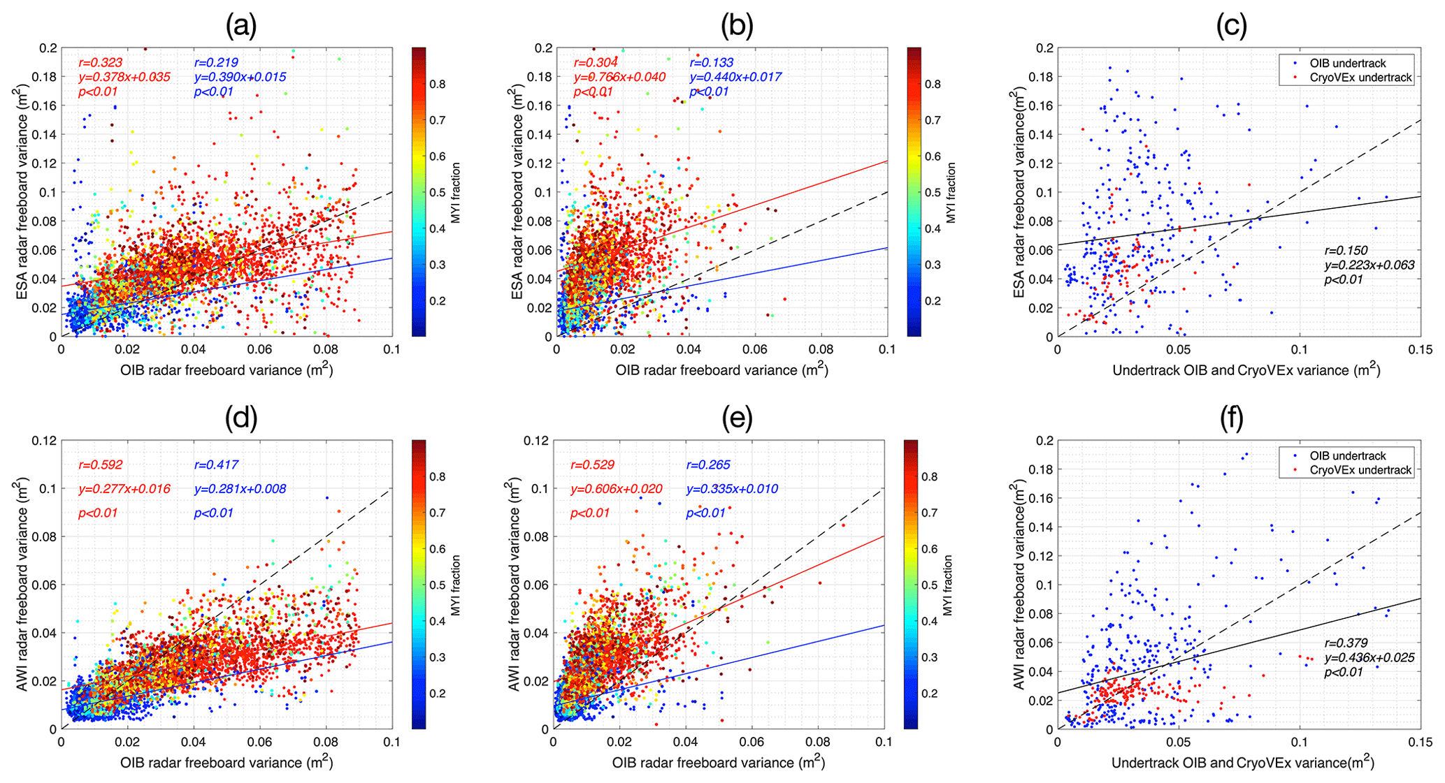
Figure 4Sample variance in Fr between OIB, CryoVEx and CS-2. Panels (a, b, c) compare ESA Fr with OIB and CryoVEx, while (d, e, f) use AWI Fr product for the comparison. Panels (a) and (d) use the sample variances as measured by original OIB resolution (40 m), while panels (b) and (e) use those of OIB on 400 m resolution (local averaging with M=10). Panels (c) and (f) show the comparison of the collocating tracks of OIB and CryoVEx with CS-2 on the scale of CS-2's along-track footprint of 400 m.
3.3 Scaling analysis of snow freeboard
In this section we compare the statistical scaling of Fs measurements by OIB and ICESat. Since there are no temporally collocating data, we compare the statistical consistency of Fs variability and scaling. Similar to Fr, the analysis of Fs scaling is also based on local regions. For comparison, ICESat attains bi-monthly basin coverage in autumn and winter, while most OIB campaigns are carried out during high winters in the western Arctic. Therefore we focus on their measurements during February, March and April in the western Arctic and differentiate between FYI and MYI. Each local region for computing the STDEV and scaling consists of about 7073 to 24 100 ICESat bi-monthly samples for each of the five winters between 2003 and 2008. Since there is no MYI fraction data product available for these years, we adopt the ice type as specified by ICESat and OIB datasets. In total, 70 673 and 96 528 local regions for FYI and MYI are recorded by ICESat. Similar to ICESat data, all OIB tracks within the same year for a local region are treated as a unit for computing STDEV.
Figure 5 shows the STDEV of Fs and its scaling. Based on the original sample resolution for both ICESat (65 m in diameter) and OIB (40 m in diameter), the modes of STDEV distribution for ICESat are 0.175 and 0.105 m for MYI and FYI, respectively, and, for OIB, they are 0.165 and 0.093 m for MYI and FYI, respectively (blue lines in Fig. 5a and c). Both OIB and ICESat show larger variability in Fs for MYI than FYI (about 50 % higher STDEV). The effective footprint for ICESat is about 3320 m2, and the area covered by OIB is lower, at 1260 m2 (see Fig. 1b). In the original footprint sizes, ICESat shows slightly higher variability. This result aligns well with the quantitative variability and uncertainty of these two products. First, after eliminating the effect of random error of ICESat (σ=5 cm) from its sample variance, the mode of STDEV distribution for ICESat is reduced from 0.175 and 0.105 to 0.168 and 0.092 m. These values are close to those observed by OIB. As previously shown in the scaling analysis, there is only a slight decrease in Fs variability from 40 to 80 m (Fig. 3c). Therefore, in the native footprints, we consider that the variability as measured by ICESat and OIB is consistent. ICESat measurements precede those of OIB by over 5 years, and we do not witness significant change in Fs variability across the Arctic Basin during this period.
In Fig. 5a and c, we also show the PDF of STDEV under local averaging. As shown, on coarser spatial scales, the overall variability in Fs drops for both OIB and ICESat. In order to accommodate the differences in footprint sizes and spatial coverage by OIB and ICESat, we study two stages for scaling analysis: (1) M=20 for OIB for comparison with M=10 for ICESat and (2) M=60 for OIB for comparison with M=30 for ICESat. For the first stage, OIB coverage is 800 m of 20 consecutive and non-overlapping “dots” of 40 m in diameter, while the ICESat footprint is 10 consecutive dots that are 1600 m apart, with each dot covering about 3300 m2. The aggregated footprint size for OIB is comparable to ICESat (25 000 m2 for OIB and 33 000 m2 for ICESat). For the first stage, the modes of STDEV for OIB and ICESat are both at 0.1 m and 0.06 m for MYI and FYI, respectively. For the second stage, the modes are 0.06 to 0.07 m (MYI) and 0.04 to 0.05 m (FYI). Here we ignore the random error's effects, since the influence on the sample STDEV is less than 2 mm for M>20.
We also compare the scaling behavior of Fs in Fig. 5b (for OIB) and Fig. 5d (for ICESat). For each local region, the slope is computed based on 40 to 1200 m (M=1 to M=30) for OIB and 65 m to 1750 m (M=1 to M=10) for ICESat. For OIB, the modes of slope PDF for MYI and FYI are −0.2 and −0.16. For ICESat, they are of similar values, at −0.2 and −0.16. Also the distribution of slopes is quite similar, with a similar standard deviation of 0.07.
As shown in Fig. 1b, OIB footprints are spatially adjacent, but for ICESat they are 175 m apart. As a consequence, the scaling analysis with local averaging is different between the two. Therefore, we study the effect of the interval between footprints of ICESat (i.e., 175 m) on OIB measurements: along-track OIB samples that are 175 m apart are extracted for the study of variability and scaling. The results are shown in Fig. 5e and f, and the sample counts (M) in Fig. 5e are aligned with Fig. 5c. While for M=1, the variability in Fs is the same as in Fig. 5a, when M is larger, the detected variability in Fs decreases faster (Fig. 5f). This indicates that when samples that are spread further are used for local averaging, the variability is more effectively dampened. With aligned spatial intervals between samples, OIB shows comparable variability to ICESat for M=10 and M=30 (Fig. 5e), and the differences between the modes of STDEV are within 1 cm.
To summarize, the general behavior of Fs scaling by ICESat and OIB is consistent, with similar values in variability and scaling behaviors. Although ICESat observations are several years before OIB campaigns, we do not observe significant changes in the variability in Fs and its scaling. It is also noted that both footprint size and spatial coverage are important for the comparison of scaling behaviors. Two factors affect the variability in Fs. First, with the increase in the aggregate footprint size, the variability decreases. Second, if the spatial coverage of samples increases while keeping the total footprint size constant, there is even more effective dampening in variability. This indicates that the portion of variability on the local scale increases with wider coverage of local samplings.
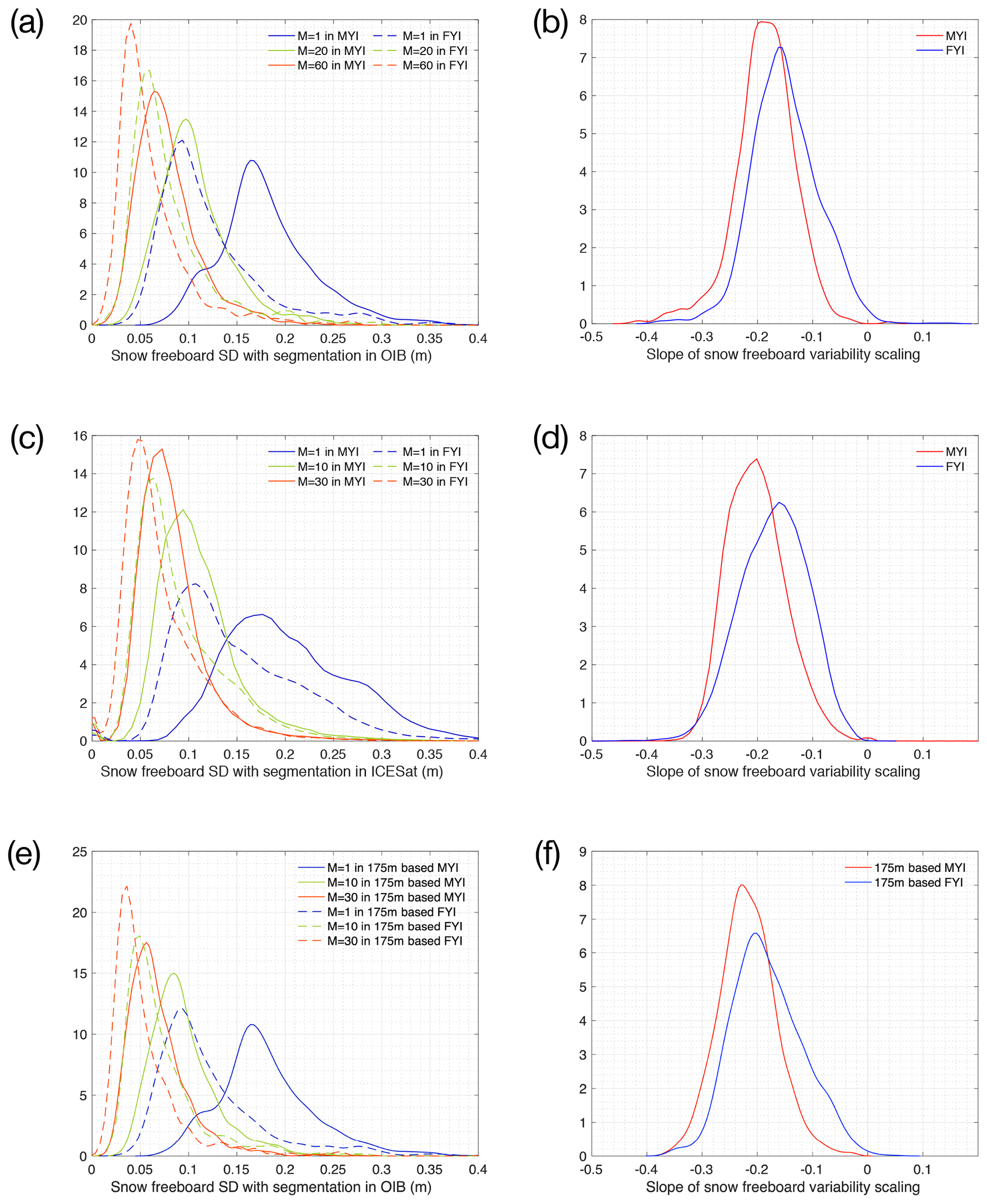
Figure 5Variability in Fs and its scaling for OIB (a, b), ICESat (c, d) and OIB, with 175 m interval (e, f) in the western Arctic.
3.4 Covariability in snow depth and freeboard
In this section we study the covariability between hs and freeboard measurements (both Fs and Fi). We mainly use OIB datasets for this analysis, since both hs and Fs are available, and they are measured and retrieved independently. The measurement errors (e and ϵ, as in Eq. 3) are formulated as below, with differentiation between the observed (denoted by |o) and inherent physical states (denoted by |p) of the parameters:
For covariability between Fs and hs, we show in Eq. (11) the deduction of covariance between Fs|p and hs|p. Hereby we assume (1) the statistical independence of errors (eATM, eSR, ϵSR and ϵATM) from physical parameters (Fs|p and hs|p), (2) the statistical independence relationships between errors and (3) no local variability in bias terms. Then we deduce that the sample covariance estimated from observations between Fs|o and hs|o is an unbiased estimator for the true, physical covariance. Figure 6 shows the PDF of sample covariance between Fs and hs for local regions with good coverage (Fig. 6a and b for 40 and 800 m, respectively). At 40 m, 95 % of all local regions show statistically significant positive covariance (hence correlation), while at 800 m, still 90 % retain positive covariance. This dominant feature is consistent with the physical perspective (Eq. 2) that the thicker snow cover induces higher total freeboard:
For Fi and hs, we also deduce the covariability as in Eq. (12). Since Fi is a derived parameter from Fs and hs in OIB, the estimation of covariance between Fi and hs may be biased by random errors. Specifically, random error in hs measurements casts a positive offset on Cov, by m2, where M is the sample count for along-track averaging. This implies that under the alternative hypothesis of negative covariance between hs and Fi, using sample covariance without this correction would increase the chance of type I error for the testing:
Figure 7a and b show the distribution of derived Cov at 40 and 800 m, respectively. On the 40 m scale, for MYI-dominated, FYI-dominated and mixed ice type regions, 97 %, 72 % and 91 % of regions show negative covariance (statistically significant at 95 % confidence level). However, at 800 m, only 30 %, 8 % and 12 % of regions show negative covariance, respectively. This result indicates that on the small scale, there is a complementary relationship between snow depth and ice freeboard. This is probably due to sea ice and snow interaction on small spatial scales. First, sea ice topographical features are more prominent on smaller spatial scales, which affects snow accumulation and results in deeper snow for local places with lower ice freeboard and thinner ice. On MYI with thicker ice and rougher topography, the negative covariability is more pronounced than in FYI. Second, since OIB campaigns are carried out during the high winters in the Arctic, thicker snow may have induced lower ice thickness growth during the whole winter, which is a potential contributor to the thinner ice and lower freeboard.
On the other hand, the disappearance of this negative correlation on larger spatial scales indicates that this phenomenon is mostly dominant on small scales. On larger scales, snow–ice interaction due to sea ice topography is less dominant, with much fewer regions showing negative covariance. Besides this, at 800 m, certain regions (about 29 % for FYI and 21 % for mixture) show significant positive covariance between Fi and hs. The difference in snowfall accumulation may be the reason: compared with younger ice, older ice (with larger Fi) is exposed to longer and heavier snowfall accumulation during autumn, resulting in thicker snow and large hs (see Fig. 4 of Boisvert et al., 2018).
Furthermore, we compute, for each local region, the spatial scale on which the negative covariance becomes statistically insignificant. For a local region, we define the critical scale (s) of snow distribution as the scale (1) on which there is statistically significant negative covariability between hs and Fi and (2) beyond which the negative covariability is not evident. For all the local regions with sufficient OIB coverage (N over 50th percentile), the distributions of s for MYI, FYI and the mixture region are shown in Fig. 7c. For FYI, about 28 % shows no negative covariance at 40 m, with the 90th percentile of s at 280 m. For MYI-dominated regions and regions with MYI and FYI mixture, a well-defined mode exists for s at 80 m and a long-tail distribution (90th percentile at 1120 and 520 m, respectively). In Fig. 7d we also show the spatial distribution of s in the Arctic Basin. As shown, large spatial variability exists in s both locally and across the basin, and regions with MYI usually feature much larger s. Regions where the roughest MYI manifests (north of Canadian Arctic Archipelago and Greenland and certain regions in Beaufort Sea with remnant MYI) show the largest s. Compared with FYI (s at about 40 m), thick MYI shows a much larger s (over 500 m for certain regions), which is evident in the snow cover's complementary effect on reducing the sea ice cover's overall variability.
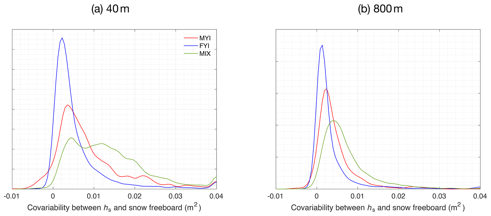
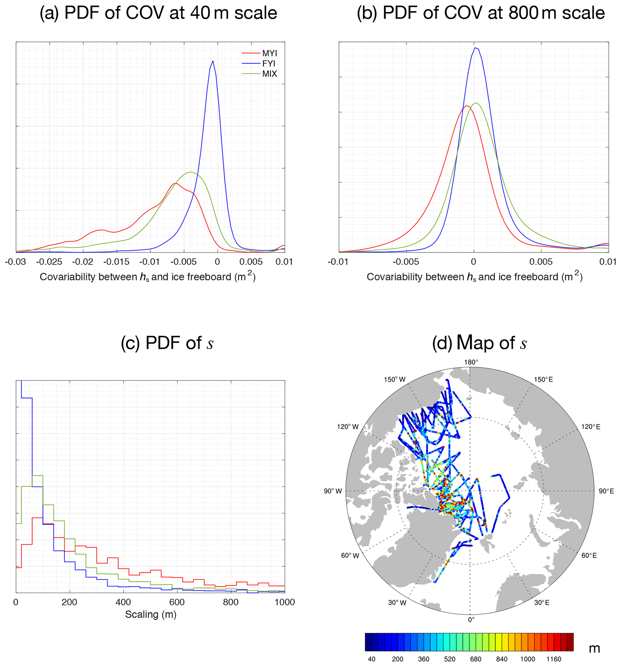
Figure 7Covariability between Fi and hs on 40 m (a) and 800 m (b) scale. Distribution of sample-estimated covariance between hs and Fi is shown (with correction for ϵSR). Critical spatial scale (s) for negative covariability between hs and Fi is shown in (c) (PDF) and (d) (geolocations).
In this article we examine the variability, its scaling and its consistency among various remote-sensing methods for Arctic sea ice, including airborne (OIB), radar altimetry (CS-2) and laser altimetry (ICESat). Analysis with collocating measurements by OIB and CS-2 shows the following: although CS-2 products contain a higher noise level on the per-sample scale, there is statistical consistency between variability in Fr as measured by OIB and CS-2. The noise level of ESA's CS-2 baseline-C Fr product is estimated at 14 to 20 cm, which is larger than current estimations. On the other hand, there is general consistency for both Fs variance and its scaling by OIB and ICESat. We do not observe significant changes of these statistics from ICESat (2004–2008) to OIB (2009 onward). Furthermore, by using OIB data, we also discovered widespread negative covariability between ice freeboard and snow depth on small spatial scales. This covariability generally diminishes on larger scales, indicating the dominant role of snow–ice interaction on local scales. The critical scale for the covariability is estimated using basin-wide OIB measurements, showing shorter ranges for FYI and much longer ranges for MYI with a long-tail distribution. The largest scale (over 500 m) is generally witnessed on the roughest MYI in the Arctic Basin.
4.1 Evaluation of variability
For the comparison between OIB and CS-2, existing works mainly focus on the consistency of the mean freeboard or ice thickness. As reported by Kurtz et al. (2014) and Xia and Xie (2018), there is low correlation of Fr between OIB and CS-2, using either gridded data or collocating tracks. Both retracking and geophysical corrections are shown to play an important role in reducing the difference (or bias) between OIB and CS-2 (Xia and Xie, 2018; Yi et al., 2018). Usually the limited representativeness is attributed as the main cause of the low correlation, which arises from differences in footprint size and spatial coverage. In this work, instead of mean values, we analyze second-order statistics (i.e., the variability) and its scaling for radar freeboards. Although CS-2 shows much higher Fr variance than OIB even on the 400 m scale, the statistically significant relationship is witnessed. This result implies that the small-scale variability in Fr can be quantitatively informed with CS-2 samples in spite of the high noise level of CS-2.
4.2 Specifics about OIB
The analysis of OIB, CS-2 and ICESat data indicates that all the factors contribute to the variability and its scaling, including measurement footprints, noise levels and spatial coverage. Except for the analysis of collocating tracks, we treat (daily) OIB campaigns and monthly CS-2 tracks as collocating sources of measurement. Since sea ice drift is prominent on the monthly scale, we also carried out analysis with CS-2 sample points under drift corrections (e.g., using NSIDC – National Snow and Ice Data Center – drift). We did not notice evident changes in the results for the analysis of variability, its scaling and the estimation of CS-2 noise levels.
As for the data independency in OIB, since Fs and hs are directly retrieved with ATM and SnowRadar, respectively, they are considered to be independent data. However, Fi, Fr and in turn hi are computed indirectly from Fs and hs. The random error in Fs and hs would cause uncertainty in both the variability and the covariability in these derived parameters. The analysis of variability scaling is less affected by random errors, since with a larger sample count the noise level decreases fast. The covariability between Fi and hs, however, can be shifted by noise in hs measurements, and the effects are accounted for by computing covariances in Sect. 3.4.
Existing works, including Kwok et al. (2017), carried out evaluation of various OIB datasets. For example, Kwok et al. (2017) show general agreement but systematic differences among hs retrievals, especially when the snow cover is thick (Figs. 4 and 5 of the reference). Since the validation showed good correlation of all hs products in Kwok et al. (2017), we consider that adopting alternative OIB datasets will not qualitatively alter the results in this study. Specifically, the products used in our study (IDCSI4 and IDCSI2) may have underestimated hs, so we expect that a thicker hs product would result in higher variability in hs as well as more evident negative covariance between Fi and hs. Comparative studies of various OIB products can be carried out in the future when they become available, following the methodology proposed in this study. In Kwok et al. (2011), it is shown that OIB SnowRadar may not be able to attain stable retrieval of snow depth over sea ice ridges. This may compromise the analysis through preferential sampling of snow depth. The effects of limited snow depth estimation over ridges is a subject of further analysis in future studies.
4.3 Effect of covariability on altimetry
The snow cover is a major source of uncertainty for both types of satellite altimetry. The variability in the measured freeboard as well as the covariability between snow depth and freeboard can be exploited to improve satellite altimetry. For laser altimetry, the positive covariability between Fs and hs is present across spatial scales (40 m to over 1 km), which covers the typical footprint size of ICESat and ICESat-2. This covariability is also reported by other works, including Kwok et al. (2011) (4 km scale) and Zhou et al. (2018) (scale ranging from 40 to 240 m). Furthermore, in Zhou et al. (2018), nonlinear fittings between hs and Fs (based on 40 m scale covariability) are utilized for the combined retrieval of hs and hi with L-band passive radiometry with laser altimetry. For laser altimetry with prescribed snow depth estimations, this positive covariability can also be utilized (1) to avoid the artificial reduction of snow depth (in favor of non-negative ice freeboard, as in Kwok and Cunningham, 2008) and (2) for the retrieval of ice thickness distribution with altimetric samples. Specifically, the covariability on the satellite sensor's footprint scale (65 m diameter for ICESat) should be utilized. On the other hand, for radar altimetry for which Fi is the major target for retrieval, the negative covariance between hs and Fi only manifests on small scales. Whether there is prevalent negative covariability at the footprint size of CS-2 is subject to further study.
Based on the statistical fitting between the variability in OIB and CS-2, we derive an indirect method in Sect. 3.2 for estimating the “real” variability on a small scale (e.g., 40 m) using CS-2 samples. Then, the mean value of freeboard (or thickness) from CS-2 can be combined with this derived variability to better inform applications that utilize CS-2 datasets. These include sea ice thickness assimilation applications (Chen et al., 2017 and Blockley and Peterson, 2018, among others), which potentially utilize mean thickness, mean freeboard and freeboard samples from CS-2. However, statistical fitting specific to the CS-2 product should be utilized, since noise levels may differ among various products (see Sect. 3.2). It is worth noting that it is not generally possible to directly estimate the freeboard distribution on a small scale with CS-2, given (1) the large footprint size of CS-2 and (2) its relatively high noise level on the per-sample scale. For example, in the N-ICE2015 campaign in King et al. (2018), which surveyed local regions with second-year ice floes mixed with first-year floes and leads, the multi-modal distribution (from high-resolution mapping) is absent in collocating CS-2 measurements (Fig. 10 of the reference). The physical features of freeboard distribution on the CS-2 footprint size, such as multi-modality, depend on the specific sea ice type (age) mixture and mixture scale of the region. In this regard, other datasets, such as synthetic-aperture radar (SAR) images, ice type mixture maps (Korosov et al., 2018) or lead (history) maps (Zhou et al., 2017), can be utilized for a more holistic view of the ice cover.
4.4 Snow–ice interaction
Negative covariability exists between Fi and hs on the small scale, which is consistent with in situ measurements. On small scales, snow cover tends to complement sea ice topography (Sturm et al., 2002a), and the main factor may be snow accumulation through its interaction with topographic features such as ridges and refrozen ponds. Besides this, snow depth also features variabilities due to snow's own processes (other than those governed by ice), such as interaction with wind. On the other hand, due to thermal insulation of snow cover, sea ice thickness growth may also be hindered by thicker snow, resulting in a “thick snow–thin ice” relationship. Compared with previous works which mainly are based on in situ measurements, this study, by utilizing OIB data, reveals the critical spatial scale for the covariability in snow distribution due to interaction with sea ice. The common spatial scale for the negative covariability is below 40 m for FYI and around 80 m with a long-tail distribution for MYI.
The understanding of the dynamical and thermodynamical mechanisms that govern the statistical behaviors would require efforts from both modeling and observational aspects. Current state-of-the-art sea ice models, including those in climate studies, usually contain major thermodynamic and dynamic processes of the sea ice cover, but many still lack snow-related ones such as snow redistribution or distribution and prognostic snow stratigraphy. Considering the complex and important roles of snow on modulating air–sea interaction (Sturm et al., 2002b; Abraham et al., 2015), snow distribution and interaction with ice topography should be accounted for by refining vertical resolution of the sea ice and snow cover as well as better parameterizations for unresolvable scales. The airborne and in situ observations, including the statistics of variability and covariability in this study, can be utilized to validate models and parameterization schemes. On the other hand, systematic observations during the freeze-up season are needed in the pursuit of quantitative attribution to the statistics in snow distribution. Multi-scale and process-oriented observational campaigns such as MOSAiC (Alfred-Wegener-Institut, 2019) could potentially shed more light on the snow cover's key processes and its complex interaction with sea ice.
OIB datasets are provided by NASA National Snow and Ice Data Center Distributed Active Archive Center, Boulder, Colorado, USA. The OIB IDCSI4 dataset is accessible at: https://doi.org/10.5067/G519SHCKWQV6 (Kurtz et al., 2015). The OIB IceBridge Sea Ice Freeboard, Snow Depth, and Thickness Quick Look dataset is accessible at: https://daacdata.apps.nsidc.org/pub/DATASETS/ICEBRIDGE/ (Kurtz and Farrell, 2011, last access: 14 September 2019). The ESA CS-2 along-track freeboard (L2i, baseline C) product is available at: https://science-pds.cryosat.esa.int/ (Bouzinac, 2014). AWI CS-2 along-track freeboard is present in the AWI CS-2 sea ice thickness (version 2.1) daily trajectory L2P product, accessible at: ftp://ftp.awi.de/sea_ice/product/cryosat2/v2p1/nh/ (Ricker et al., 2014, last access: 14 September 2019). CryoVEx is from ESA Earth Observation Campaigns, accessed at: ftp://calval-pds.cryosat.esa.int/ (Haas et al., 2009, last access: 14 September 2019). ICESat data are provided by NASA National Snow and Ice Data Center Distributed Active Archive Center, Boulder, Colorado, USA, at: https://doi.org/10.5067/SXJVJ3A2XIZT (Yi and Zwally, 2009).
SX designed the work. LZ and SX collected and processed the data. SX and LZ carried out the analysis. All authors contributed to the writing of the paper.
The authors declare that they have no conflict of interest.
The authors would like to thank the editors and referees for their invaluable efforts in improving the paper. The authors would also like to thank the data providers for opening access to CryoSat-2, ICESat, Operation IceBridge and CryoVEx datasets.
This research has been supported by the National Key R&D Program of China (grant no. 2017YFA0603902) and the National Natural Science Foundation of China (grant no. 41575076).
This paper was edited by John Yackel and reviewed by three anonymous referees.
Abraham, C., Steiner, N., Monahan, A., and Michel, C.: Effects of subgrid-scale snow thickness variability on radiative transfer in sea ice, J. Geophys. Res.-Oceans, 120, 5597–5614, https://doi.org/10.1002/2015JC010741, 2015. a
Alfred-Wegener-Institut: MOSAiC Expedition, available at: https://www.mosaic-expedition.org, last access: 6 February 2019. a
Armitage, T. W. K. and Ridout, A. L.: Arctic sea ice freeboard from AltiKa and comparison with CryoSat-2 and Operation IceBridge, Geophys. Res. Lett., 42, 6724–6731, https://doi.org/10.1002/2015GL064823, 2015. a
Blockley, E. W. and Peterson, K. A.: Improving Met Office seasonal predictions of Arctic sea ice using assimilation of CryoSat-2 thickness, The Cryosphere, 12, 3419–3438, https://doi.org/10.5194/tc-12-3419-2018, 2018. a, b
Boisvert, L. N., Webster, M. A., Petty, A. A., Markus, T., Bromwich, D. H., and Cullather, R. I.: Intercomparison of Precipitation Estimates over the Arctic Ocean and Its Peripheral Seas from Reanalyses, J. Climate, 31, 8441–8462, https://doi.org/10.1175/JCLI-D-18-0125.1, 2018. a
Bouzinac, C.: CryoSat-2 product handbook, London, UK, ESRIN-ESA and Mullard Space Science Laboratory, University College London, available at: https://earth.esa.int/documents/10174/125272/CryoSat_Product_Handbook (last access: 13 September 2019), 2014. a
Cavalieri, D. J., Parkinson, C. L., Gloersen, P., Comiso, J. C., and Zwally, H. J.: Deriving long-term time series of sea ice cover from satellite passive-microwave multisensor data sets, J. Geophys. Res.-Oceans, 104, 15803–15814, 1999. a
Chen, Z., Liu, J., Song, M., Yang, Q., and Xu, S.: Impacts of Assimilating Satellite Sea Ice Concentration and Thickness on Arctic Sea Ice Prediction in the NCEP Climate Forecast System, J. Climate, 30, 8429–8446, https://doi.org/10.1175/JCLI-D-17-0093.1, 2017. a, b
Haas, C., Lobach, J., Hendricks, S., Rabenstein, L., and Pfaffling, A.: Helicopter-borne measurements of sea ice thickness, using a small and lightweight, digital EM system, J. Appl. Geophys., 67, 234–241, https://doi.org/10.1016/j.jappgeo.2008.05.005, 2009. a, b
Haas, C., Hendricks, S., Eicken, H., and Herber, A.: Synoptic airborne thickness surveys reveal state of Arctic sea ice cover, Geophys. Res. Lett., 37, L09501, https://doi.org/10.1029/2010GL042652, 2010. a
King, J., Skourup, H., Hvidegaard, S. M., Rösel, A., Gerland, S., Spreen, G., Polashenski, C., Helm, V., and Liston, G. E.: Comparison of Freeboard Retrieval and Ice Thickness Calculation From ALS, ASIRAS, and CryoSat-2 in the Norwegian Arctic to Field Measurements Made During the N-ICE2015Expedition, J. Geophys. Res.-Oceans, 123, 1123–1141, https://doi.org/10.1002/2017JC013233, 2018. a, b
Korosov, A. A., Rampal, P., Pedersen, L. T., Saldo, R., Ye, Y., Heygster, G., Lavergne, T., Aaboe, S., and Girard-Ardhuin, F.: A new tracking algorithm for sea ice age distribution estimation, The Cryosphere, 12, 2073–2085, https://doi.org/10.5194/tc-12-2073-2018, 2018. a, b
Krabill, W. B.: Pre-IceBridge ATM L1B Qfit Elevation and Return Strength, Boulder, Colorado USA: NASA DAAC at the National Snow and Ice Data Center. https://doi.org/10.5067/DZYN0SKIG6FB, updated 2013, 2009. a
Kurtz, N. T. and Farrell, S. L.: Large-scale surveys of snow depth on Arctic sea ice from Operation IceBridge, Geophys. Res. Lett., 38, L20505, https://doi.org/10.1029/2011GL049216, 2011. a
Kurtz, N., Studinger, M., Harbeck, J., Onana, V.-D.-P., and Farrell, S.: IceBridge Sea Ice Freeboard, Snow Depth, and Thickness, available at: http://nsidc.org/data/idcsi2.html (last access: 24 February 2020), updated each year, 2012. a
Kurtz, N., Studinger, M., Harbeck, J., Onana, V., and Yi, D.: IceBridge L4 Sea Ice Freeboard, Snow Depth, and Thickness, Version 1, https://doi.org/10.5067/G519SHCKWQV6, 2015. a, b, c
Kurtz, N. T., Farrell, S. L., Studinger, M., Galin, N., Harbeck, J. P., Lindsay, R., Onana, V. D., Panzer, B., and Sonntag, J. G.: Sea ice thickness, freeboard, and snow depth products from Operation IceBridge airborne data, The Cryosphere, 7, 1035–1056, https://doi.org/10.5194/tc-7-1035-2013, 2013. a, b, c, d
Kurtz, N. T., Galin, N., and Studinger, M.: An improved CryoSat-2 sea ice freeboard retrieval algorithm through the use of waveform fitting, The Cryosphere, 8, 1217–1237, https://doi.org/10.5194/tc-8-1217-2014, 2014. a, b
Kwok, R. and Cunningham, G. F.: ICESat over Arctic sea ice: Estimation of snow depth and ice thickness, J. Geophys. Res.-Oceans, 113, c08010, https://doi.org/10.1029/2008JC004753, 2008. a, b, c, d, e, f
Kwok, R., Panzer, B., Leuschen, C., Pang, S., Markus, T., Holt, B., and Gogineni, S.: Airborne surveys of snow depth over Arctic sea ice, J. Geophys. Res.-Oceans, 116, C11018, https://doi.org/10.1029/2011JC007371, 2011. a, b
Kwok, R., Kurtz, N. T., Brucker, L., Ivanoff, A., Newman, T., Farrell, S. L., King, J., Howell, S., Webster, M. A., Paden, J., Leuschen, C., MacGregor, J. A., Richter-Menge, J., Harbeck, J., and Tschudi, M.: Intercomparison of snow depth retrievals over Arctic sea ice from radar data acquired by Operation IceBridge, The Cryosphere, 11, 2571–2593, https://doi.org/10.5194/tc-11-2571-2017, 2017. a, b, c
Laxon, S. W., Giles, K. A., Ridout, A. L., Wingham, D. J., Willatt, R., Cullen, R., Kwok, R., Schweiger, A., Zhang, J., Haas, C., Hendricks, S., Krishfield, R., Kurtz, N., Farrell, S., and Davidson, M.: CryoSat-2 estimates of Arctic sea ice thickness and volume, Geophys. Res. Lett., 40, 732–737, https://doi.org/10.1002/grl.50193, 2013. a
Leuschen, C.: IceBridge Snow Radar L1B Geolocated Radar Echo Strength Profiles, Version 2, Boulder, Colorado USA, NASA National Snow and Ice Data Center Distributed Active Archive Center, https://doi.org/10.5067/FAZTWP500V70, 2014 (updated 2017). a
Lindell, D. B. and Long, D. G.: Multiyear Arctic Sea Ice Classification Using OSCAT and QuikSCAT, IEEE T. Geosci. Remote, 54, 167–175, https://doi.org/10.1109/TGRS.2015.2452215, 2016. a
Martin, C. F., Krabill, W. B., Manizade, S., Russell, R., Sonntag, J. G., Swift, R. N., and Yungel, J. K.: Airborne Topographic Mapper Calibration Procedures and Accuracy Assessment, NASA Technical Reports, Tech. rep., Natl. Aeronaut. and Space Admin, Washington, D. C., available at: http://hdl.handle.net/2060/20120008479 (last access: 24 February 2020), 2012. a
Nandan, V., Geldsetzer, T., Yackel, J., Mahmud, M., Scharien, R., Howell, S., and Else, B.: Effect of snow salinity on CryoSat-2 Arctic first-year sea ice freeboard measurements, Geophys. Res. Lett., 44, 419–426, https://doi.org/10.1002/2017GL074506, 2017. a
Parrinello, T., Shepherd, A., Bouffard, J., Badessi, S., Casal, T., Davidson, M., Fornari, M., Maestroni, E., and Scagliola, M.: CryoSat: ESA's ice mission – eight years in space, Adva. Space Res., 62, 1178–1190, https://doi.org/10.1016/j.asr.2018.04.014, 2018. a
Resti, A., Benveniste, J., Roca, M., Levrini, G., and Johannessen, J.: The Envisat Radar Altimeter System (RA-2), ESA Bulletin, 98, available at: http://www.esa.int/esapub/bulletin/bullet98/RESTI.PDF (last access: 24 February 2020), 1999. a
Ricker, R., Hendricks, S., Helm, V., Skourup, H., and Davidson, M.: Sensitivity of CryoSat-2 Arctic sea-ice freeboard and thickness on radar-waveform interpretation, The Cryosphere, 8, 1607–1622, https://doi.org/10.5194/tc-8-1607-2014, 2014. a, b, c, d, e, f
Ricker, R., Hendricks, S., Perovich, D. K., Helm, V., and Gerdes, R.: Impact of snow accumulation on CryoSat-2 range retrievals over Arctic sea ice: An observational approach with buoy data, Geophys. Res. Lett., 4447–4455, https://doi.org/10.1002/2015GL064081, 2015. a
Stroeve, J., Barrett, A., Serreze, M., and Schweiger, A.: Using records from submarine, aircraft and satellites to evaluate climate model simulations of Arctic sea ice thickness, The Cryosphere, 8, 1839–1854, https://doi.org/10.5194/tc-8-1839-2014, 2014. a
Sturm, M., Holmgren, J., and Perovich, D. K.: Winter snow cover on the sea ice of the Arctic Ocean at the Surface Heat Budget of the Arctic Ocean (SHEBA): Temporal evolution and spatial variability, J. Geophys. Res.-Oceans, 107, 8047, https://doi.org/10.1029/2000JC000400, 2002a. a
Sturm, M., Perovich, D. K., and Holmgren, J.: Thermal conductivity and heat transfer through the snow on the ice of the Beaufort Sea, J. Geophys. Res.-Oceans, 107, SHE 19–1–SHE 19–17, https://doi.org/10.1029/2000JC000409, 2002b. a
Tilling, R. L., Ridout, A., Shepherd, A., and Wingham, D. J.: Increased Arctic sea ice volume after anomalously low melting in 2013, Nat. Geosci., 8, 643–646, 2015. a
Tilling, R. L., Ridout, A., and Shepherd, A.: Estimating Arctic sea ice thickness and volume using CryoSat-2 radar altimeter data, Adv. Space Res., 62, 1203–1225, 2017. a, b
Warren, S. G., Rigor, I. G., Untersteiner, N., Radionov, V. F., Bryazgin, N. N., Aleksandrov, Y. I., and Colony, R.: Snow Depth on Arctic Sea Ice, J. Climate, 12, 1814–1829, https://doi.org/10.1175/1520-0442(1999)012<1814:SDOASI>2.0.CO;2, 1999. a, b
Webster, M., Gerland, S., Holland, M., Hunke, E., Kwok, R., Lecomte, O., Massom, R., Perovich, D., and Sturm, M.: Snow in the changing sea-ice systems, Nat. Clim. Change, 8, 946–953, https://doi.org/10.1038/s41558-018-0286-7, 2018. a
Webster, M. A., Rigor, I. G., Nghiem, S. V., Kurtz, N. T., Farrell, S. L., Perovich, D. K., and Sturm, M.: Interdecadal changes in snow depth on Arctic sea ice, J. Geophys. Res.-Oceans, 119, 5395–5406, https://doi.org/10.1002/2014JC009985, 2014. a
Wingham, D., Francis, C., Baker, S., Bouzinac, C., Brockley, D., Cullen, R., de Chateau-Thierry, P., Laxon, S., Mallow, U., Mavrocordatos, C., Phalippou, L., Ratier, G., Rey, L., Rostan, F., Viau, P., and Wallis, D.: CryoSat: A mission to determine the fluctuations in Earth's land and marine ice fields, Adv. Space Res., 37, 841–871, https://doi.org/10.1016/j.asr.2005.07.027, 2006. a, b
Xia, W. and Xie, H.: Assessing three waveform retrackers on sea ice freeboard retrieval from Cryosat-2 using Operation IceBridge Airborne altimetry datasets, Remote Sens. Environ., 204, 450–471, https://doi.org/10.1016/j.rse.2017.10.010, 2018. a, b, c
Ye, Y., Shokr, M., Heygster, G., and Spreen, G.: Improving Multiyear Sea Ice Concentration Estimates with Sea Ice Drift, Remote Sensing, 8, 5. Article 397, https://doi.org/10.3390/rs8050397, 2016. a
Yi, D. and Zwally, H. J.: Arctic Sea Ice Freeboard and Thickness, Version 1, Boulder, Colorado USA. NSIDC: National Snow and Ice Data Center, https://doi.org/10.5067/SXJVJ3A2XIZT, 2009. a, b
Yi, D., Kurtz, N., Harbeck, J., Kwok, R., Hendricks, S., and Ricker, R.: Comparing Coincident Elevation and Freeboard From IceBridge and Five Different CryoSat-2 Retrackers, IEEE T. Geosci. Remote, 57, 1219–1229, https://doi.org/10.1109/TGRS.2018.2865257, 2018. a, b, c, d
Zhou, L., Xu, S., Liu, J., Lu, H., and Wang, B.: Improving L-band radiation model and representation of small-scale variability to simulate brightness temperature of sea ice, Int. J. Remote Sens., 38, 7070–7084, https://doi.org/10.1080/01431161.2017.1371862, 2017. a
Zhou, L., Xu, S., Liu, J., and Wang, B.: On the retrieval of sea ice thickness and snow depth using concurrent laser altimetry and L-band remote sensing data, The Cryosphere, 12, 993–1012, https://doi.org/10.5194/tc-12-993-2018, 2018. a, b
Zygmuntowska, M., Rampal, P., Ivanova, N., and Smedsrud, L. H.: Uncertainties in Arctic sea ice thickness and volume: new estimates and implications for trends, The Cryosphere, 8, 705–720, https://doi.org/10.5194/tc-8-705-2014, 2014. a