the Creative Commons Attribution 4.0 License.
the Creative Commons Attribution 4.0 License.
 | 17 Feb 2020
Parameter sensitivity analysis of dynamic ice sheet models – numerical computations
Per Lötstedt
The friction coefficient and the base topography of a stationary and a dynamic ice sheet are perturbed in two models for the ice: the full Stokes equations and the shallow shelf approximation. The sensitivity to the perturbations of the velocity and the height at the surface is quantified by solving the adjoint equations of the stress and the height equations providing weights for the perturbed data. The adjoint equations are solved numerically and the sensitivity is computed in several examples in two dimensions. A transfer matrix couples the perturbations at the base with the perturbations at the top. Comparisons are made with analytical solutions to simplified problems. The sensitivity to perturbations depends on their wavelengths and the distance to the grounding line. A perturbation in the topography has a direct effect at the ice surface above it, while a change in the friction coefficient is less visible there.
- Article
(2637 KB) - Full-text XML
- BibTeX
- EndNote


The output of isothermal simulations of large ice sheets depends on the ice model, the topography, and the parametrization of the conditions at the base of the ice. The models are systems of partial differential equations (PDEs) for the velocity, pressure, and height of the ice. The boundary conditions of the PDEs are given by the topography and the friction model with its parameters. Of particular interest in the simulation of ice is the horizontal velocity and the height at the ice surface. In the inverse problem, the parameters at the base are inferred from data at the surface by solving adjoint equations and minimizing the difference between given data and simulated results. In this paper, we estimate the sensitivity of the surface observations to changes in the basal conditions by solving the adjoint equations to the full Stokes (FS) equations and the shallow shelf (or shelfy stream) approximation (SSA) (see Greve and Blatter, 2009; MacAyeal, 1989). The advantage of solving the adjoint equations in a variational control method is that the effect of many perturbations of the parameters at the bottom is obtained for one observation at one point of the surface at a certain time point. If there are many observations and only one perturbation, then it is more efficient to compute the sensitivity by solving the forward model PDEs twice in a direct method – firstly with the unperturbed parameters and secondly with the perturbed parameters – and then take the difference between the solutions. The direct method has the advantage that there is no need to implement a solver for the adjoint equations.
We are interested in the effect of perturbations of the topography and the slipperiness at the ice base on the velocity of the ice at the surface and its height. By solving the adjoint equations, we quantify the sensitivity to perturbations close to the grounding line and of different wavelengths. The sensitivity at the upper surface to perturbations in the basal topography and friction is different, and the separation of the two contributions appears to be difficult. The transfer functions between the perturbations at the base and the surface observations are more or less well behaved. A related problem is to infer the basal geometry and friction coefficients from observational data by inversion using the adjoint solution.
Most methods for inversion of ice surface data to compute parameters in the models at the ice base rely on a solution of the adjoint stress equation with a given fixed geometry of the ice as in MacAyeal (1993) for SSA and in Petra et al. (2012) for FS, where the time-dependent height equation for the moving upper surface is not included in the inversion. The stationary basal friction coefficients have been derived from satellite data in this way for many glaciers and continental ice sheets using velocity data in, e.g., Gillet-Chaulet et al. (2016), Isaac et al. (2015), Schannwell et al. (2019), and Sergienko and Hindmarsh (2013).
The conditions between the ice and the bedrock vary in time, and sometimes the friction parameter varies several orders of magnitude in a decade (see, e.g., Jay-Allemand et al., 2011). In addition, there are variations on seasonal and diurnal time scales with examples in Schoof (2010), Shannon et al. (2013), and Vallot et al. (2017). Other time-dependent forces are considered in Seddik et al. (2019). The effect of a seasonal variation of the lubrication at the base of the ice is studied in Shannon et al. (2013) for the Greenland ice sheet by solving the FS and other high-order equations. Fast temporal variations in the meltwater under the ice drive the ice flow in the analysis in Schoof (2010). The spatial and temporal variations of the basal conditions are inferred from satellite data in Larour et al. (2014) with an inverse method for SSA and automatic differentiation. Based on observations, the conclusion in Sole et al. (2011) is also that the annual change in the water drainage under the ice affects the sliding and the acceleration and deceleration of the ice. Transient data are included in Goldberg et al. (2015) to find time-dependent basal parameters by inversion, where the sensitivity is determined by automatic differentiation. The results differ if the time evolution of the equations is taken into account or not. The shallow ice approximation (SIA) is the ice model in Monnier and des Boscs (2017) to determine the basal properties with time-dependent surface data. Here, we solve the adjoint equations to both the stress equation and the time-dependent height equation in FS and SSA to examine how the dynamics of the models change the sensitivity to the base parameters. The adjoint equations are derived and analytical solutions are found to simplified equations in a companion paper by Cheng and Lötstedt (2019). The influence of the dynamics of the basal conditions is different on the velocity and the height observations.
The forward advection equation for the height and the stress equations for the velocity for FS are here solved numerically in two dimensions (2-D) with Elmer/Ice (Gagliardini et al., 2013; Gillet-Chaulet et al., 2012). The solver of the adjoint stress equation in Elmer/Ice is amended by the adjoint height equation. The forward and adjoint SSA equations are solved for a vertical ice in 2-D by a finite difference method. The perturbations are observed in the velocity and the height at certain points in space and time. Comparisons are made for steady-state and time-dependent problems between a direct calculation of the change at the ice surface and using the control technique with the adjoint solution. Simplified adjoint stress equations have been proposed and used in Martin and Monnier (2014), Morlighem et al. (2013), and Mosbeux et al. (2016). The sensitivity in the SSA model is evaluated in this paper for such simplifications in the adjoint SSA equations. The sensitivity in the numerical solutions is also compared to the analytical formulas in Cheng and Lötstedt (2019). It is observed in Durand et al. (2011) that the sensitivity to changes at the base increases closer to the grounding line in the coastal regions. The basal topography is inferred from the height data in van Pelt et al. (2013) without solving the adjoint equations. The reason for the increased sensitivity and why the height method works are explained by our analytical solutions to the adjoint SSA equations.
There is a transfer matrix between the perturbations in the parameters at the base and the observations at the surface. Analytical expressions for time-dependent transfer functions for FS and SSA are derived in Gudmundsson (2003, 2008) by linearizing, freezing coefficients, and applying Fourier analysis and the Laplace transform. The properties of the transfer matrix are evaluated here to see which combinations of perturbations and observations are well- and ill-conditioned. In an ill-conditioned problem, the sensitivity at the surface to perturbations at the base is low. This matrix can also be used to quantify the uncertainty in the ice flow due to uncertainties in the model parameters (see, e.g., Bulthuis et al., 2019; Schlegel et al., 2018; Smith, 2014). Perturbations at the ice base with short wavelength are propagated to the surface with a weaker effect on the height and velocity compared to long wavelengths in Gudmundsson (2003, 2008). These are the conclusions in calculations with FS in Kyrke-Smith et al. (2018), where it is difficult to separate the contribution from the friction and the bed topography from each other. These effects are confirmed in our analysis.
The structure of the paper is as follows. The ice equations and the corresponding adjoint equations for FS and SSA are presented in Sect. 2. The computed sensitivities are compared between the direct method and the control method in Sect. 3 for steady-state and time-dependent problems in 2-D. The ice configuration is taken from the MISMIP benchmark project in Pattyn et al. (2012). The results are discussed and conclusions are drawn in Sects. 4 and 5. Formulas from Cheng and Lötstedt (2019) are found in Appendix A.
Vectors and matrices are written in bold as a and A. The operations and ⋆ on vectors a and c, matrices A and C, and four index tensors 𝒜 are defined by
The definition of a norm of a vector a is .
The equations of two ice models and their adjoint equations are stated in this section. The FS equations are considered to be an accurate model of ice sheets, and the SSA equations are an approximation of the FS equations suitable, e.g., for fast flowing ice on the ground and ice floating on water (see Greve and Blatter, 2009).
2.1 Full Stokes equations
The FS equations are a system of PDEs for the velocity of the ice , the pressure p(x,t), and the height with the coordinates and time t. There is a stress equation satisfied by u and p and an advection equation for h. The adjoint equation of the stress equation is derived in Petra et al. (2012), and the adjoint equations of the stress and the height equations are found in Cheng and Lötstedt (2019). The sensitivity of observations of the velocity and the height of the ice surface is derived for perturbations in the friction coefficient at the ice base.
The domain of the ice is Ω with boundary Γ in three dimensions (3-D). The boundary consists of the ice surface at the upper boundary Γs, the lower boundary at the ice base Γb and Γw, and the vertical and lateral boundaries Γu and Γd, where Γu is the upstream boundary with and Γd is the downstream boundary with . The normal of Γ pointing outward is denoted by n. The projection of Γs and Γb on the horizontal x–y plane is ω and the projections of Γu and Γd are γu and γd, respectively. The z coordinate of the grounded base Γb is the topography and the bathymetry b(x,y). The grounding line γGL separates Γb on ω from Γw floating on water with a moving z coordinate . Formal definitions of these domains are
Let I be the identity matrix. The projection of a vector on the tangential plane of Γb is denoted by as in Petra et al. (2012). In 2-D, and γd=L.
2.1.1 Forward equations
The definitions of the strain rate D and the viscosity η of the ice are
The trace of D2 is trD2 and the rate factor A depends on the temperature of the ice, here assumed to be constant in isothermal flow. The material constant n>0 is given in Glen's flow law. Then the stress tensor is
Let ρ be the density of the ice, g be the gravitational acceleration, and a be the accumulation/ablation rate on the surface Γs. The notation is simplified with the slope vectors in 3-D and in 2-D. A subscript or t on a variable denotes a partial derivative such that . Then the forward FS equations for and p are
The initial data for h are h0(x), and hγ(x,t) is specified on the inflow boundary γu. The expression Cf(Tu) defines the friction law with variable coefficient C(x,t) and a function f(⋅) of the projected velocity Tu, e.g., as in Weertman (1957), where
The Dirichlet boundary conditions of u on Γu and Γd are set to be uu and ud.
2.1.2 Adjoint equations
We observe a quantity
at the surface Γs when . For example, if the ice is in the steady state and with the Dirac delta (δ), then the observation is the x component of u at x∗:
If then the height is observed as
The adjoint equations depend on the first variations Fu and Fh of F(u,h) with respect to u and h. In the first example above, and Fh=0, and in the second example Fu=0 and .
The adjoint FS equations form a system of PDEs for the adjoint height ψ, the adjoint velocity v, and the adjoint pressure q. There is an advection equation for ψ and an adjoint stress equation for v and q such that
where the adjoint viscosity, adjoint stress, and linearized friction law in Eq. (8) are according to Petra et al. (2012):
The tensor ℐ with four indices ijkl is 1 when and 0 otherwise.
The perturbation of the observation in Eq. (7) with respect to a perturbation in the friction coefficient C is
involving the tangential projections of the forward and adjoint velocities Tu and Tv at the grounded ice base Γb. This expression is derived in Cheng and Lötstedt (2019) and Petra et al. (2012) via the perturbation of the Lagrangian of the system of equations and by evaluating it at the forward and adjoint solutions.
Only perturbations in C are considered here for the FS model. Via the Lagrangian, the result of perturbations δb in the topography can be derived, but the complexity of the adjoint Eq. (8) would increase considerably.
2.2 Shallow shelf approximation
In the shallow shelf approximation of the FS equations, the velocity is constant in the vertical direction and the pressure is given by the cryostatic approximation (Greve and Blatter, 2009; MacAyeal, 1989). The sensitivity of observations of the velocity at the surface and the height to perturbations in friction coefficients and the base topography is quantified for the SSA model.
2.2.1 Forward equations
It is sufficient to solve for the horizontal velocity when , thus simplifying the 3-D FS problem Eq. (5) considerably. The viscosity in the SSA is
where . The stress tensor ς(u) in SSA is defined by
Let n be the outward normal vector of the boundary γ, t the tangential vector such that , and the thickness of the ice. The friction law is defined as in the FS case in Eq. (6), where the basal velocity is replaced by the horizontal velocity since the vertical variation is neglected in SSA. Under the floating ice shelf on Γw, C=0 in the friction law.
The ice dynamics system is
where uin≤0 and uout>0 are the inflow and outflow normal velocities on γu and γd of the boundary . The friction on the lateral side of the ice depends on the tangential velocity t⋅u there. The friction law Cγfγ(t⋅u) on γg is not necessarily the same as Cf(u) on ω.
The structure of the SSA system Eq. (13) is similar to the FS equations in Eq. (5). However, the velocity u is not divergence-free in SSA and B≠D due to the cryostatic approximation.
2.2.2 Adjoint equations
The adjoint SSA equations are derived in Cheng and Lötstedt (2019) as in Sect. 2.1.2 by forming the Lagrangian and partial integration using the forward equations and the boundary conditions in Eq. (13). The adjoint viscosity and adjoint stress are defined by
cf. and in Eq. (9). The adjoint SSA equations are
Compared to Eq. (8), the advection equation depends on v, and the influence of ψ in the stress equation is different in Eq. (15). With a Weertman friction law Eq. (6), the terms Fω and Fγ in the adjoint basal friction and the lateral friction in Eq. (15) are
The friction coefficients on the base and the lateral sides are perturbed by δC and δCγ, and the topography is perturbed by δb in the SSA model. Then the perturbation δℱ in the observation ℱ in Eq. (7) is (Cheng and Lötstedt, 2019)
2.2.3 Forward and adjoint SSA in 2-D
In the 2-D model, u2=0, derivatives with respect to y vanish, and the lateral friction force is neglected, Cγ=0. The ice domains are the grounded and floating parts and , where xGL is the position of the grounding line. The friction coefficient C is positive on Γb and C=0 on Γw. The forward and adjoint equations in 2-D are derived from Eqs. (13) and (15) by letting H and u1 be independent of y and taking u2=0. The notation is simplified if we let u=u1 and v=v1. The forward equations follow from Eq. (13):
Assume that u>0 and ux>0. There is an inflow of ice with speed uL to the left and a calving rate uc at x=L. The viscosity in Eq. (11) is simplified to . The friction term is Cf(u)u=Cum with the Weertman law in Eq. (6).
The adjoint variables v and ψ satisfy the adjoint equations in 2-D:
obtained from Eqs. (14) and (15) or derived from Eq. (17) with equal result.
Perturbations δb and δC in the topography and the friction coefficient propagate to the surface as in Eq. (16):
2.2.4 Discretized relations in 2-D
In order to simplify the notation, only a 2-D steady-state problem for the SSA model is considered here, but the analysis is applicable to 3-D steady-state problems as well as time-dependent problems with the FS or SSA models.
The time-independent perturbation of ℱ in Eq. (19) for the steady-state solution is rewritten with and weights wub and wuC:
The weights wub and wuC in Eq. (20) depend on both x∗ and x. When h is observed the perturbation is
where the weights whb and whC have the same form as in Eq. (20) but with different ψ and v.
The relation is discretized by observing u at equidistant with , and perturbing b and C at with . The integral in Eq. (20) is computed by the trapezoidal rule to have
or in matrix form
with the matrix elements
In the same manner, there are matrices Whb and WhC connecting δh with δb and δC:
The sensitivity of u to changes in b and C on ω is given by the singular value decomposition (SVD) of Wub and WuC (Golub and Van Loan, 1989) defined by
where Uub and UuC are of size M×M and Vub and VuC are of size N×N. A summary of the properties of the SVD is found in the Appendix.
Consider the case when δb=0 in Eq. (23). The relation between δu and δC is well behaved in Eq. (23) if all the singular values σuCi of WuC are of similar size, but if some of them are much smaller than the other ones with then the relation is ill-conditioned. A large perturbation in C may then result in a hardly visible perturbation at the surface, and a small observed perturbation in u may correspond to a large perturbation at the base. The same conclusions apply to Wub and σubi in the relation between δu and δb and to the sensitivity matrices Whb and WhC when .
The transfer functions in Gudmundsson (2003, 2008) between perturbations in b and C at the base and the observations u and h at the top are determined by linearization and Fourier transformation in a slab geometry. The transfer function for different wave numbers corresponds to the singular values in our analysis.
2.2.5 Relation to the inverse problem
The sensitivity problem and the inverse problem are related. Assume that there are M observations of the velocity uobs at the surface of the ice at xi and we want to derive the corresponding friction coefficient C at j locations. With C we observe u at the top at the same coordinates. Then we seek a correction δC of C at N points such that u+δu approaches uobs. Using Eq. (23),
and δC is chosen such that is minimized. This problem is a linear-least-squares problem. Expressed with the SVD and the generalized inverse , the solution is
see Golub and Van Loan (1989) and the Appendix. The solution can be improved iteratively with updates of C and u by and , computing a new WuC and so on.
The relation between the transfer matrix and the inversion problem is illustrated by Eq. (26), but a more efficient optimization method is based on the gradient of the objective function . It is the standard method for inversion in, e.g., Gillet-Chaulet et al. (2016), Isaac et al. (2015), and Petra et al. (2012), and the gradient is computed using the adjoint solution with .
In the numerical experiments we use a 2-D constant downward-sloping bed with an ice profile from the MISMIP benchmark project in Pattyn et al. (2012). The bedrock elevation in meters is given as
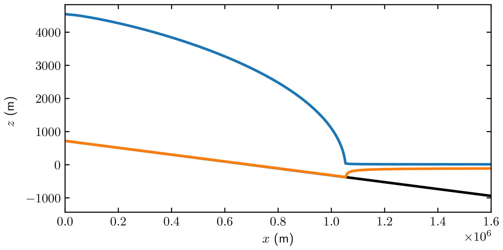
Figure 1The initial ice geometry with height h (blue), ice base b (orange), and ocean bathymetry (black). The domains in Eq. (2) are the ice domain Ω between the blue and orange curves, the upper surface Γs in blue, the lower boundary on the bedrock Γb and on water Γw in orange, Γu at x=0, and Γd at m.
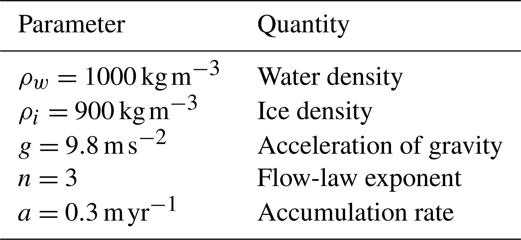
The initial configuration of the ice is a steady-state solution achieved by the FS model using Elmer/Ice (Gagliardini et al., 2013) with , with a grounding line position at m shown in Fig. 1. The Weertman-type friction law in Eq. (6) in the forward problem has the exponent and a constant friction coefficient . The remaining physical parameters are given in Table 1.
Without losing the generality in the friction law and to investigate the relation between the basal velocity and the stress, the friction law exponent in the adjoint problem is assumed to be m=1, and the coefficient is calculated from the forward steady-state solution by . The resulting friction law becomes Cf(u)=C(x), which can be viewed as a linearization of the friction law at the steady state.
3.1 Full Stokes model
A vertically extruded mesh is constructed for the given geometry with mesh size Δx=1 km yielding equidistant nodes in the horizontal direction. The number of vertical layers is set to 20 in the whole domain. Only the grounded ice is considered in the adjoint problem, and Dirichlet boundary conditions on u are used for the lateral boundaries Γd and Γu at the grounding line x=xGL and the ice divide x=0.
The forward and adjoint FS problems are solved using the finite element code Elmer/Ice (Gagliardini et al., 2013) with a P1–P1 quadrilateral element and Galerkin least-squares stabilization for the Stokes equation and a bubble stabilization (Baiocchi et al., 1993) for the adjoint advection equation. The feature to solve the adjoint time-dependent equations has been added to Elmer/Ice. The Dirac delta is approximated by a linear basis function with the amplitude 1∕Δx.
The time-stepping scheme for the forward and adjoint transient problems is the implicit Euler method with a constant time step Δt=1 year. The adjoint equation is solved backward in time from the final time t=T to t=0. The steady state of the adjoint equations is computed by neglecting the time derivative term in the adjoint surface equation Eq. (8) and solving the corresponding linear system of equations for ψ and v.
Both transient and steady-state simulations are run with pointwise observations of the horizontal velocity u1 and surface elevation h at different x∗ positions on the top surface. The time interval for the transient solutions is [0,1], covered by one forward time step Δt from 0 to 1 and one backward time step from 1 to 0.
The multiplier ψ only acts as the amplitude of the external force on Γs, and h is an approximate normal vector pointing inward on Γs in the adjoint FS equation Eq. (8). The size of ψh is several orders of magnitude smaller than 1, which is equivalent to the coefficient in front of in Fu. Consequently, in the u1-response case, the adjoint solution v is mainly influenced by the observation function Fu. However, in the h-response case with Fu=0, the adjoint solution v is determined by ψh and the solution would be v=0 if we did not solve the adjoint advection equation for ψ.

Figure 2Comparison of the weights Tu⋅Tv in Eq. (10) for perturbations δC at different observation points , and 0.9×10⁶ (blue, orange, green, and pink). (a, b) Transient simulations; (c, d) steady states. (a, c) wuC with pointwise u response; (b, d) whC with pointwise h response.
The adjoint solutions v1 at Γb of all the four cases are concentrated at the observation points. The vertical component v2 shares the same feature as v1 due to the boundary condition on Γb. Therefore, the weights Tu⋅Tv in Fig. 2 are also confined to the neighborhood of x∗. The negative weights obtained in the u1-response cases imply that an increase in the basal friction coefficient results in a decrease in the surface velocity. The amplitude of the weights grows rapidly toward the grounding line in all four cases in the figure. In fact, the contribution of the weight function to the observed variables u1 can be viewed as a convolution of the perturbation in C(x) with a narrow Gaussian in Eq. (20) after a proper scaling in the left panels of Fig. 2.
The amplitude of the perturbation at the surface depends on the wavelength λ of the perturbation at the base. The shorter λ is, the smaller the amplitude is. Introduce a stationary perturbation with a constant C0 and a small ϵ≪1. Then the change in the steady-state solution u1 at the surface is according to Eq. (10)
The same relation holds for δh(x∗) but with a different v. Let ϱ be a measure of the width of the weight function for the steady state in Fig. 2, which is about 105. When λ is large compared to ϱ then
which is a constant value for long λ, and the perturbation can be observed at the surface. If the wavelength of the basal perturbation is short compared to ϱ, then it is damped before it reaches the surface, and the effect of δC on u1 and h is small. In Fig. 3, and are compared at . When λ>ϱ then . Suppose that . Then is about and probably hard to observe and . Similar conclusions are drawn theoretically in Gudmundsson (2003, 2008) using Fourier analysis and experimentally in Sun et al. (2014).
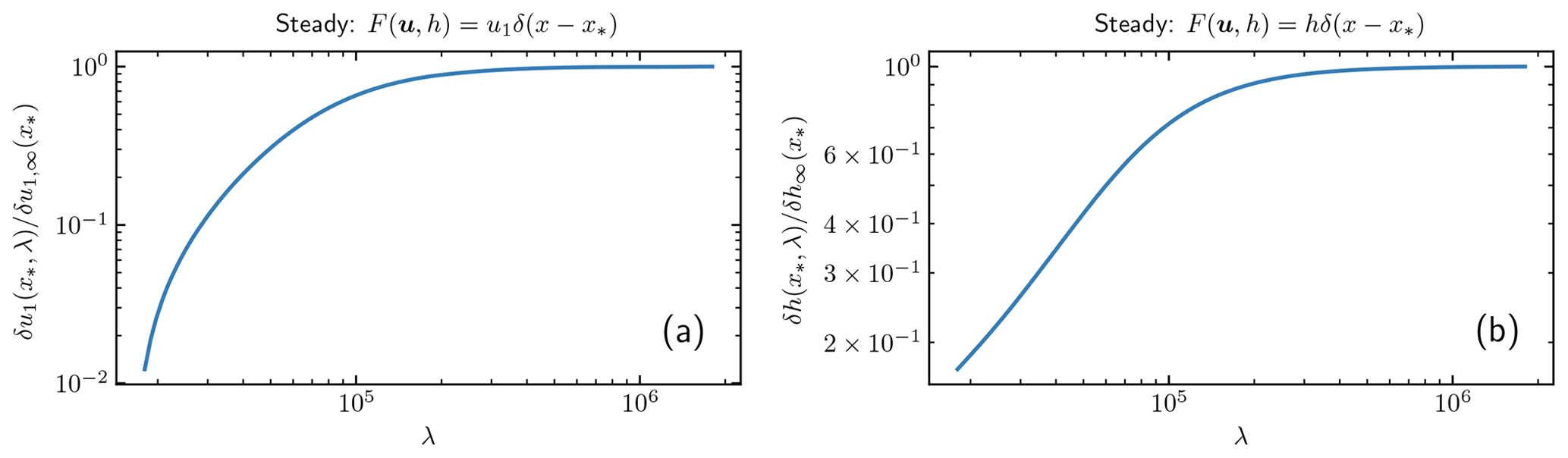
Figure 3The response at Γs with different wavelengths λ in the perturbation of C in Eq. (28). (a) ; (b) .
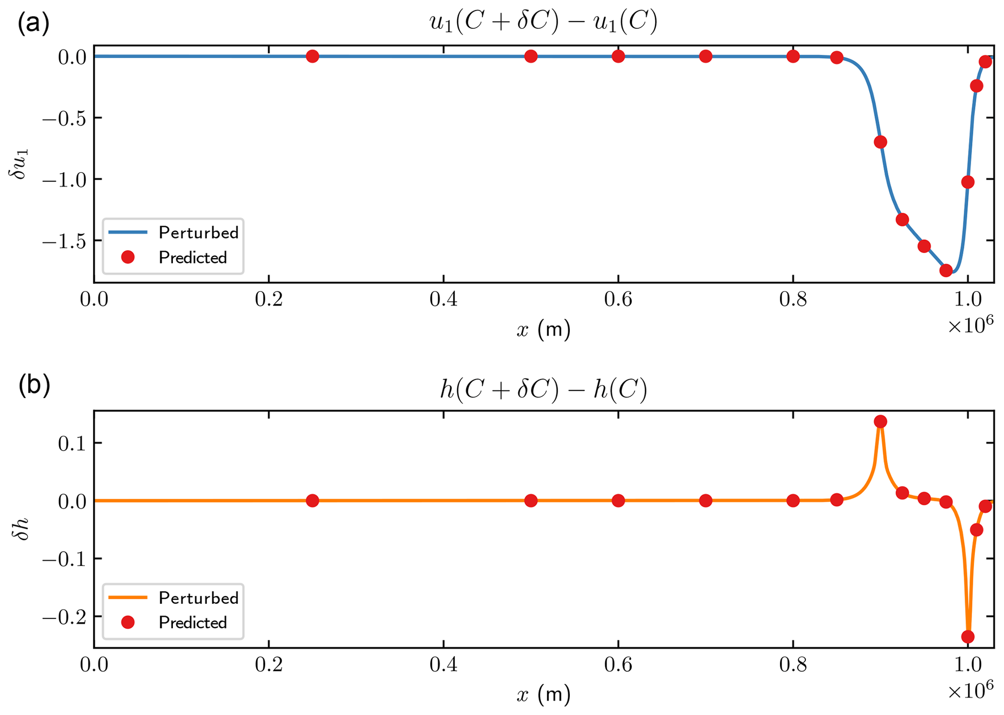
We perform a pair of experiments to compare the results from perturbing the forward equation and the prediction by the adjoint solutions. A relative 1 % perturbation δC(x) is added at m to the friction coefficient C(x). The differences between the forward FS solutions with and without the perturbation after 1 year are shown in Fig. 4 marked as “perturbed”. The predicted perturbations are computed from the solutions of the adjoint equation by varying x∗ along the x axis and inserting it into Eq. (10). Each red dot in Fig. 4 corresponds to one single observation at x∗. Both the u1 and h predictions are in good agreement with the forward perturbations.
3.2 SSA
The same MISMIP benchmark experiment as in Sect. 3.1 is solved by the SSA on a one-dimensional uniform grid with mesh size Δx=1 km using standard finite difference methods implemented in MATLAB. The time derivatives are discretized by the implicit Euler method with a constant time step Δt=1 year as in Sect. 3.1. An upwind scheme is used for the spatial derivatives in the forward and adjoint advection equations to stabilize the numerical solutions. Replacing the Dirac delta with a Gaussian distribution function a few grid points wide in order to smoothen the observation function and avoid numerical oscillations in the solution has no major effect on the solutions.
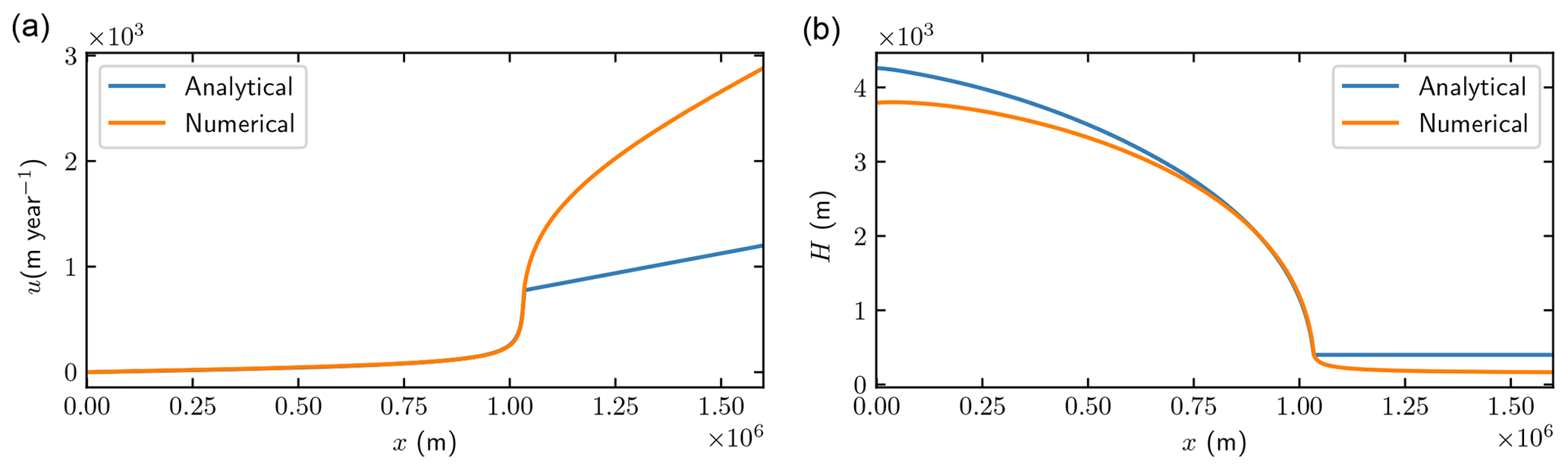
The numerical solution of the forward SSA equations Eq. (17) is compared to the analytical approximations in the Appendix Eq. (A1) in Fig. 5. The detailed derivations of the analytical solutions in the Appendix are found in Cheng and Lötstedt (2019). The analytical approximation of u is poor to the right of xGL for the floating ice in Fig. 5, but we are only interested in the solution for the grounded ice. The reason for the error in the analytical solution of u is that H is assumed to be constant for x>xGL. The analytical solution for H catches the fast decrease when x approaches xGL from the left. Another solution for x>xGL is found in Greve and Blatter (2009) assuming that the thickness depends linearly on x.
The weight functions wuC and whC in Fig. 6 have the same nonzero pattern as v since they are equal to −vum in Eq. (20). Each one of these weights wuC or whC corresponds to the sensitivity of the observation at x∗ with respect to the change in C(x), which is one row in the weight matrices WuC or WhC in Eqs. (23) and (24). The analytical weight functions in Eqs. (A3) and (A5) at m are included in the steady-state figures for comparison. In the transient SSA simulations, the sensitivity is similar to those in the adjoint FS solutions in Fig. 2 increasing towards the grounding line. Such an increased sensitivity is also noted in Kyrke-Smith et al. (2018) and Leguy et al. (2014). However, in the steady-state cases, the weight functions indicate only an upstream effect of C(x). In other words, the perturbation in C(x) at point x can only influence the steady-state solutions to the left of this point. This is true as long as the effect of the grounding line migration is neglected. The δC weights for u responses are all negative, implying that an increase in C leads to decrease in u, but the steady-state surface elevation h rises when C is increased. The weights for the transient problem have a similar shape for the FS and SSA models in Figs. 2 and 6.
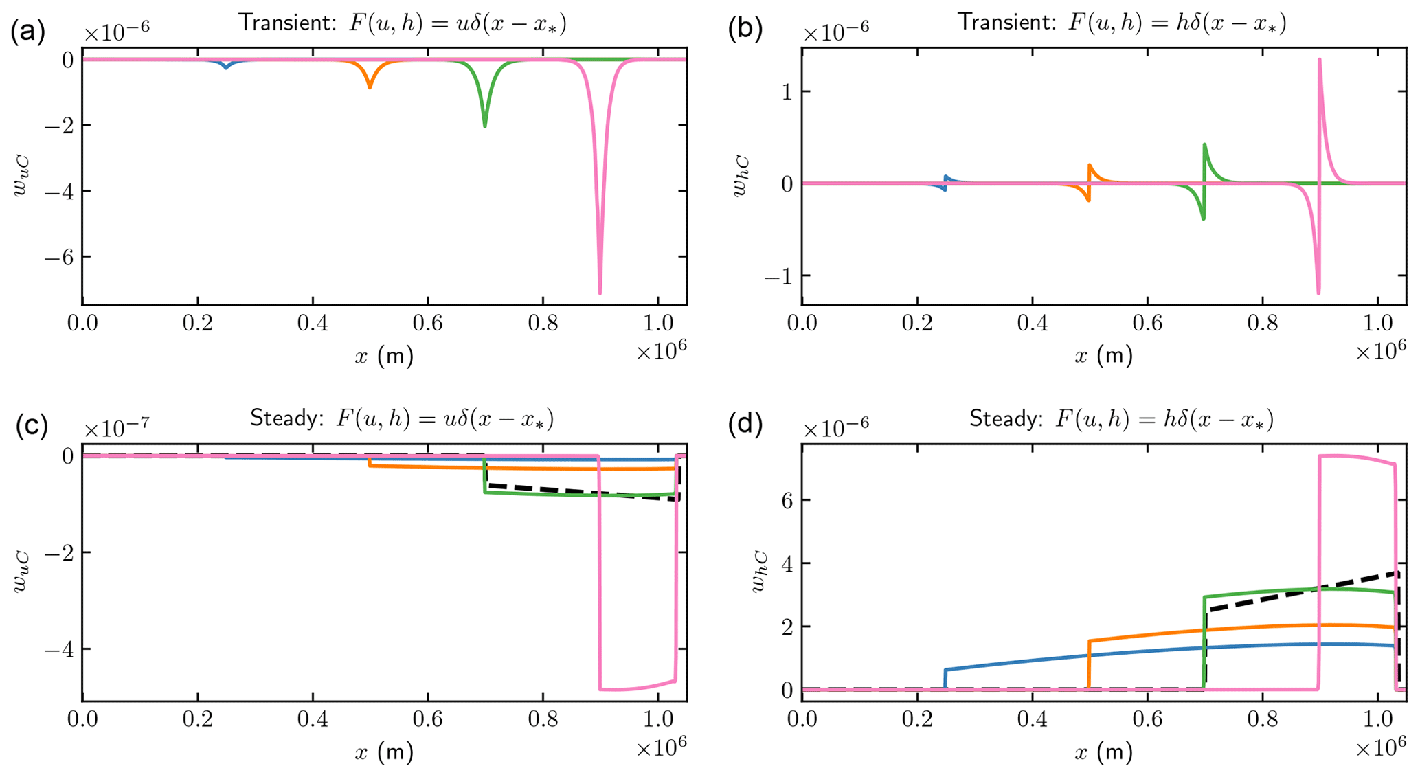
Figure 6Comparison of the weights wuC and whC for SSA in Eq. (19) for perturbations δC with m=1 at different observation points , and 0.9×10⁶ (blue, orange, green, and pink). The dashed black lines in (c, d) are wuC and whC computed from the analytical solutions of u in Eq. (A1) and v in Eqs. (A2) and (A4) at . (a, b) Transient simulations; (c, d) steady states. (a, c) wuC for pointwise u response; (b, d) whC for pointwise h response.
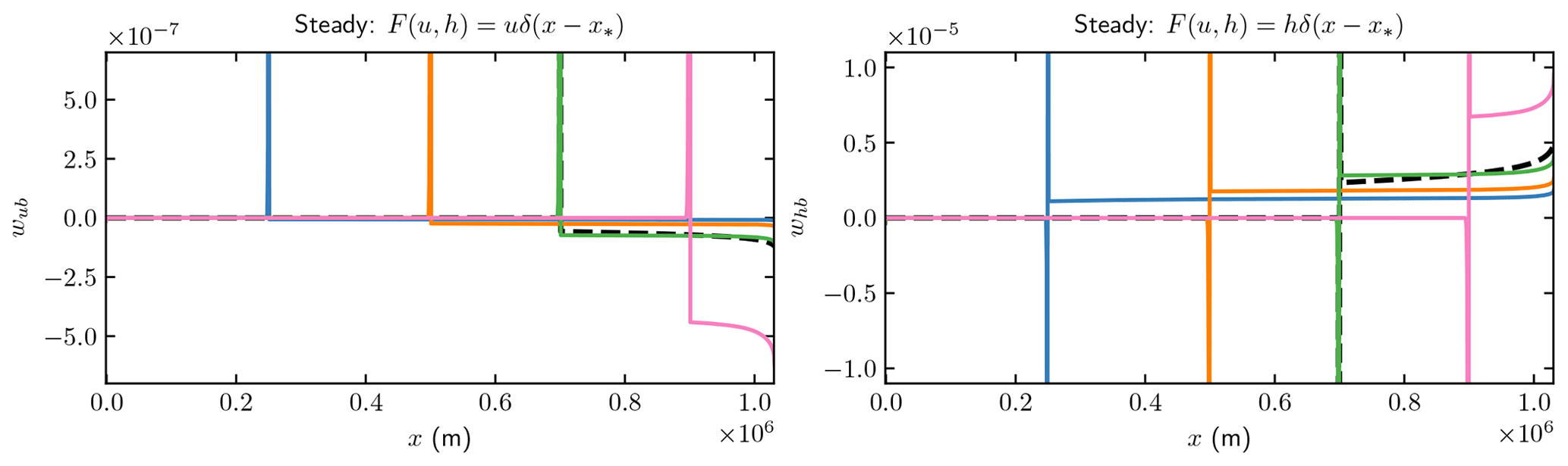
The weight functions wub and whb for δb are localized at the observation position x∗ in all the four cases in Fig. 7, which implies that the inverse problems may be well-posed. The dashed black lines in the two lower panels are the analytical expressions of the weight functions at m in Eqs. (A3) and (A5) with a hat function of width 2Δx at the base to approximate the Dirac delta. The analytical solutions almost coincide with the numerical solutions. The steady-state weight functions are nonzero to the right of x∗, corresponding to the integral in Eq. (A5). There is a detailed view of the steady-state δb weights for in Fig. 8. The weights of δb have similar structures to the δC weights. The analytical solutions in Eqs. (A3) and (A5) suggest that for .
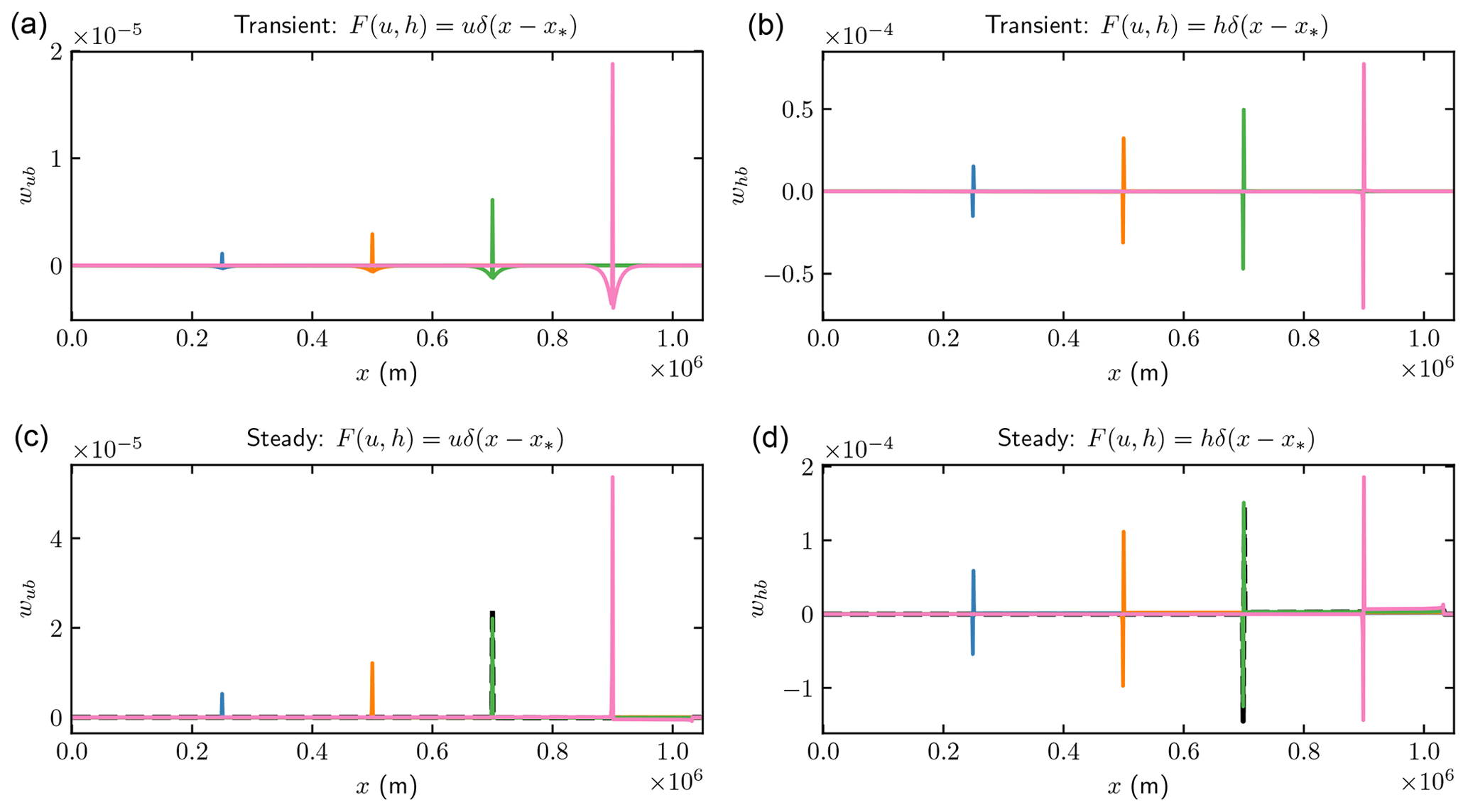
Figure 7Comparison of the weights wub and whb for SSA in Eq. (19) for perturbations δb at different observation points , and 0.9×10⁶ (blue, orange, green, and pink). The dashed black lines in (c, d) are the weights of δb in Eqs. (A3) and (A5) at . (a, b) Transient simulations; (c, d) steady states. (a, c) wub for pointwise u response; (b, d) whb for pointwise h response.
The same perturbation on C(x) as in Fig. 4 is imposed in the SSA simulations. The perturbed solutions after 1 year and 15 000 years (which is close to a steady state) are computed with the forward equations, and then the reference solutions at the steady state without any perturbation are subtracted. This difference is compared to the perturbations obtained with the adjoint equations as in Fig. 4. In the 1-year perturbation experiment in Fig. 10, the transient weight functions in the upper panels in Fig. 6 are used for the sensitivity estimates. The weight functions in the upper panels of Fig. 7 predict the response in Fig. 11.
The corresponding comparisons for the steady-state problem are made in Figs. 12 and 13 with the weights in the lower panels of Figs. 6 and 7. The analytical solutions of the steady-state perturbations from Eqs. (A3) and (A5) are shown with dashed black lines in these two figures.
The rapid change in δh in Figs. 10 and 11 is explained by the shape of the weight functions in the upper-right panels of Figs. 6 and 7. The weights can be approximated by for some θ>0. Then the surface response will be
where δC jumps discontinuously at and . The same phenomenon is found for FS in Fig. 4 with an explanation in Fig. 2.
The perturbations δu and δh in the steady state in Fig. 12 have discontinuous derivatives δux and δhx where δC has jumps. This is explained by the integral terms in Eqs. (A3) and (A5). The discontinuities in the upper panel of Fig. 13 are caused by the jumps in δb at 0.9×10⁶ and 1.0×10⁶ and the first term in Eq. (A3). The jumps in δh in the lower panel of Fig. 13 are due to the first term in Eq. (A5).
All the predicted solutions from the adjoint SSA are in good agreement with the forward perturbation.
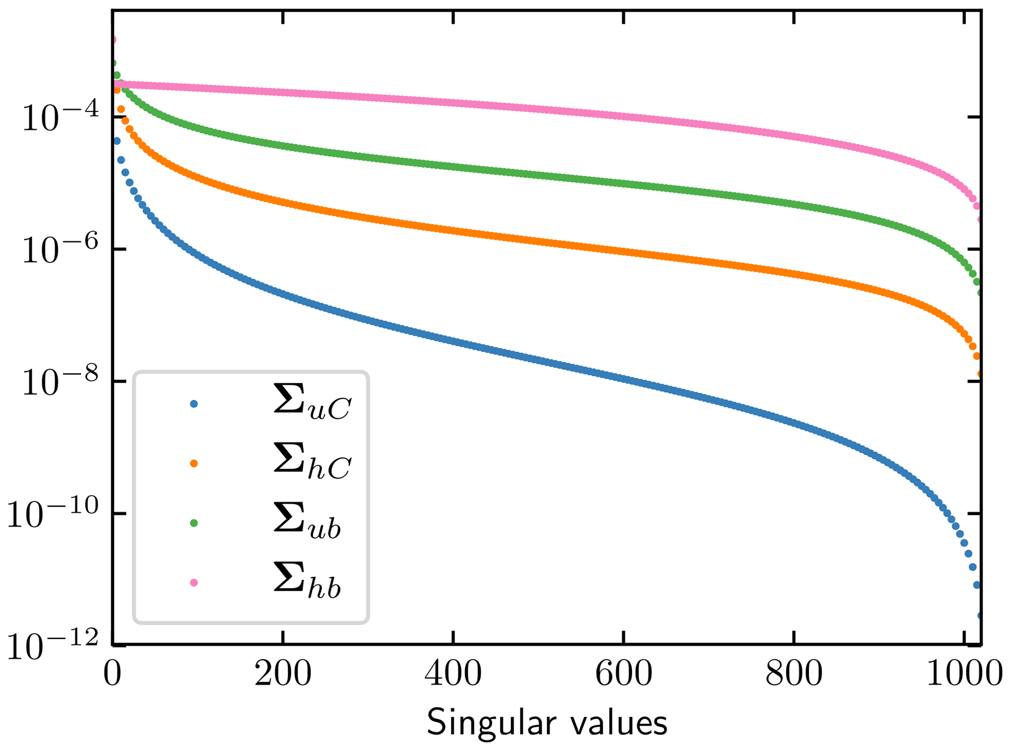
The inverse problem of the steady state for the friction coefficient may not be well-posed since the weights are all positive from x∗ to xGL. This is verified by checking the singular values of the sensitivity matrices WuC and WhC in Fig. 9, where the largest and smallest singular values of ΣuC are 10−4 and 10−12 with a large quotient σuC1∕σuCN and the span of the singular values of ΣhC is from 10−4 to 10−8 (which is better).
The singular values of the sensitivity matrices Wub and Whb in Fig. 9 are in the interval 10−4 to 10−7 from large to small. They are better conditioned than the sensitivity matrices for C. In particular, Σhb (in pink) in the h-response case has the lowest variation of the singular values. The inverse problem of solving for the topography b from the surface elevation h in the steady-state setup is a well-posed problem compared to inferring C from u.
Good approximations of the sensitivity matrices WuC, WhC, Wub, and Whb are found in Eqs. (A3) and (A5) at given x∗i and xj as in Eq. (23). If the basal topography is unperturbed at the same x coordinate as the observation point such that , then the contributions of δb and δC cannot be separated since they are both multiplied by the same weight except for a different scaling factor. This is in agreement with numerical investigations in Kyrke-Smith et al. (2018). It is shown in Cheng and Lötstedt (2019) that the perturbation in δu is proportional to the wavelength of δC. Perturbations with short wavelengths will not reach the surface. These conclusions are also drawn in numerical solutions of FS in Kyrke-Smith et al. (2018) and with transfer functions in the frequency space in Gudmundsson (2008). The perturbation in u due to δC increases with increasing u and decreasing H. The sensitivity of δu and δh behaves in a better way if the observation at x∗ is above the perturbation at x in the topography in Eqs. (A3) and (A5). Then δb and its derivative directly affect the perturbations at the top of the ice. This is in agreement with the computed singular values in Fig. 9. This property is utilized in van Pelt et al. (2013) when the bottom topography is inferred from height data. Inferring the geometry of the base from such data is easier than inferring the slipperiness and C because of the first term in Eq. (A5) and whb in the right column of Fig. 7.
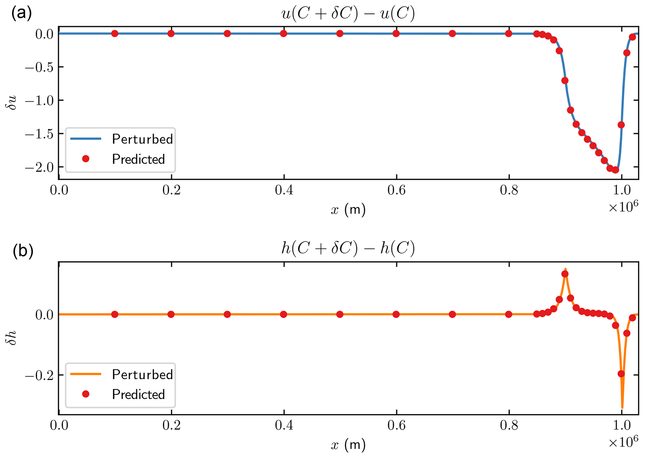
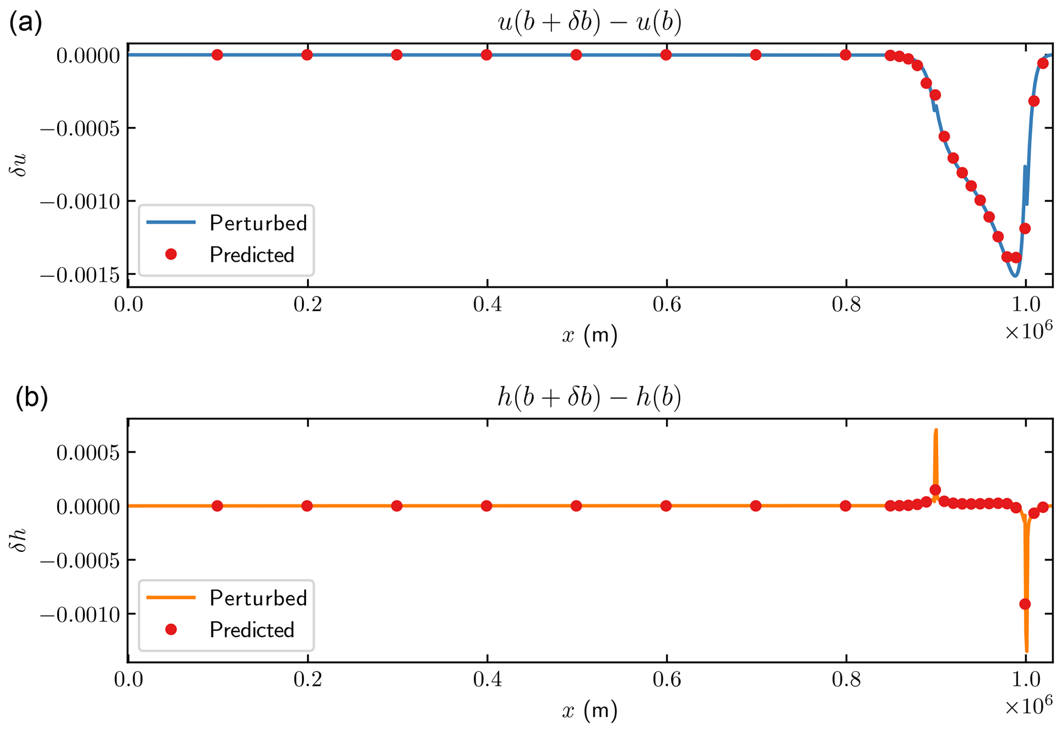
Figure 11The changes in the horizontal velocity u (a) and surface elevation h (b) for SSA after 1 year with 0.01 m perturbation of b(x) in m. Solid lines are the differences between the steady-state and the perturbed solutions in Eq. (13). Red dots represent the estimated perturbation using Eq. (15).
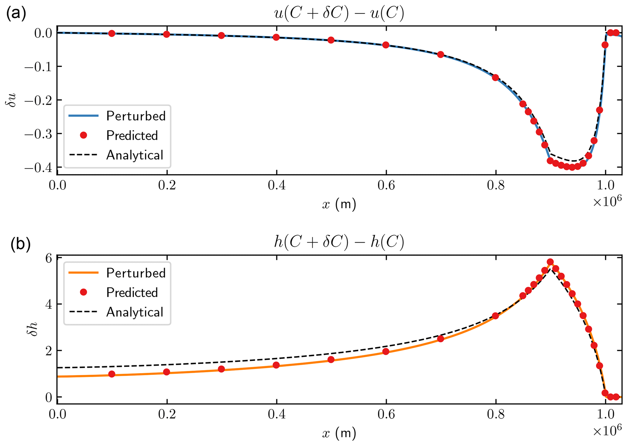
Figure 12The changes in the horizontal velocity u (a) and surface elevation h (b) for SSA after 15 000 years (close to the steady state) with 1 % perturbation of C(x) in . Solid lines are the differences between the steady-state and perturbed solutions in Eq. (13). Red dots represent the estimated perturbation using Eq. (15).
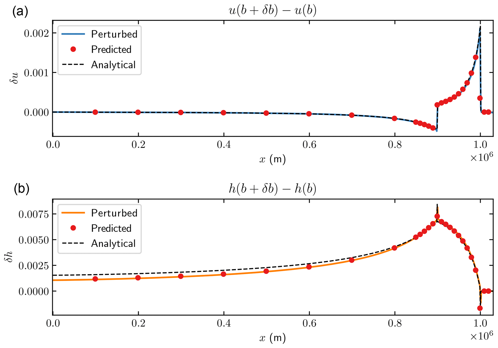
Figure 13The changes in the horizontal velocity u (a) and surface elevation h (b) for SSA after 15 000 years (close to the steady state) with 0.01 m perturbation of b(x) in . Solid lines are the differences between the steady-state and perturbed solutions in Eq. (13). Red dots represent the estimated perturbation using Eq. (15).
The solution of the adjoint equations is simplified in the comparison in Fig. 14. In MacAyeal (1993), two simplifications are made. Firstly, the adjoint viscosity in Eq. (14) is approximated by the forward viscosity η in Eq. (11). The factor 1∕n in the viscosity in the 2-D stress equation Eq. (18) is then replaced by 1. Secondly, the thickness H is fixed and the advection equation for ψ is not solved, which is equivalent to ∇ψ=0 in the adjoint stress equation in Eq. (15). Perturbations are introduced in C and u is observed for the transient case as in Fig. 10. The perturbed forward solutions are compared to the predicted perturbations by the simplified adjoint SSA systems in Fig. 14, where the forward viscosity η is used in both cases. In the upper panel of Fig. 14, the two equations of ψ and v are solved. In the lower panel, the advection equation of ψ is excluded from the system. The differences are small in this case compared to the full adjoint solution used in Fig. 10. The reason is that and Hηux are small in Eq. (18).
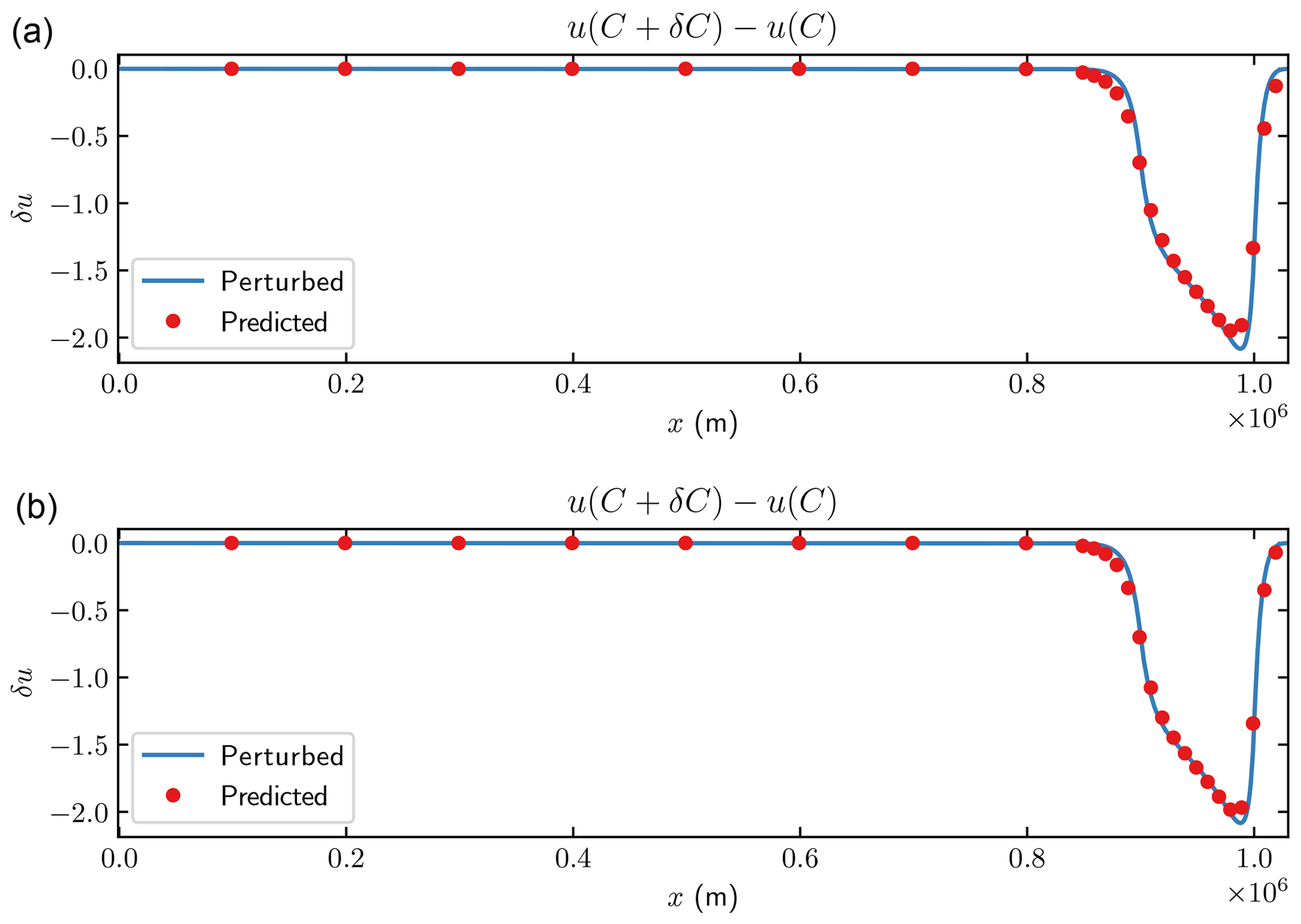
Figure 14The changes in the horizontal velocity u for SSA after 1 year with 1 % perturbation of C(x) in m. Solid lines are the differences between the steady-state and the perturbed solutions in Eq. (13). Red dots represent the estimated perturbation using Eq. (15). (a) Forward viscosity. (b) Without advection equation.
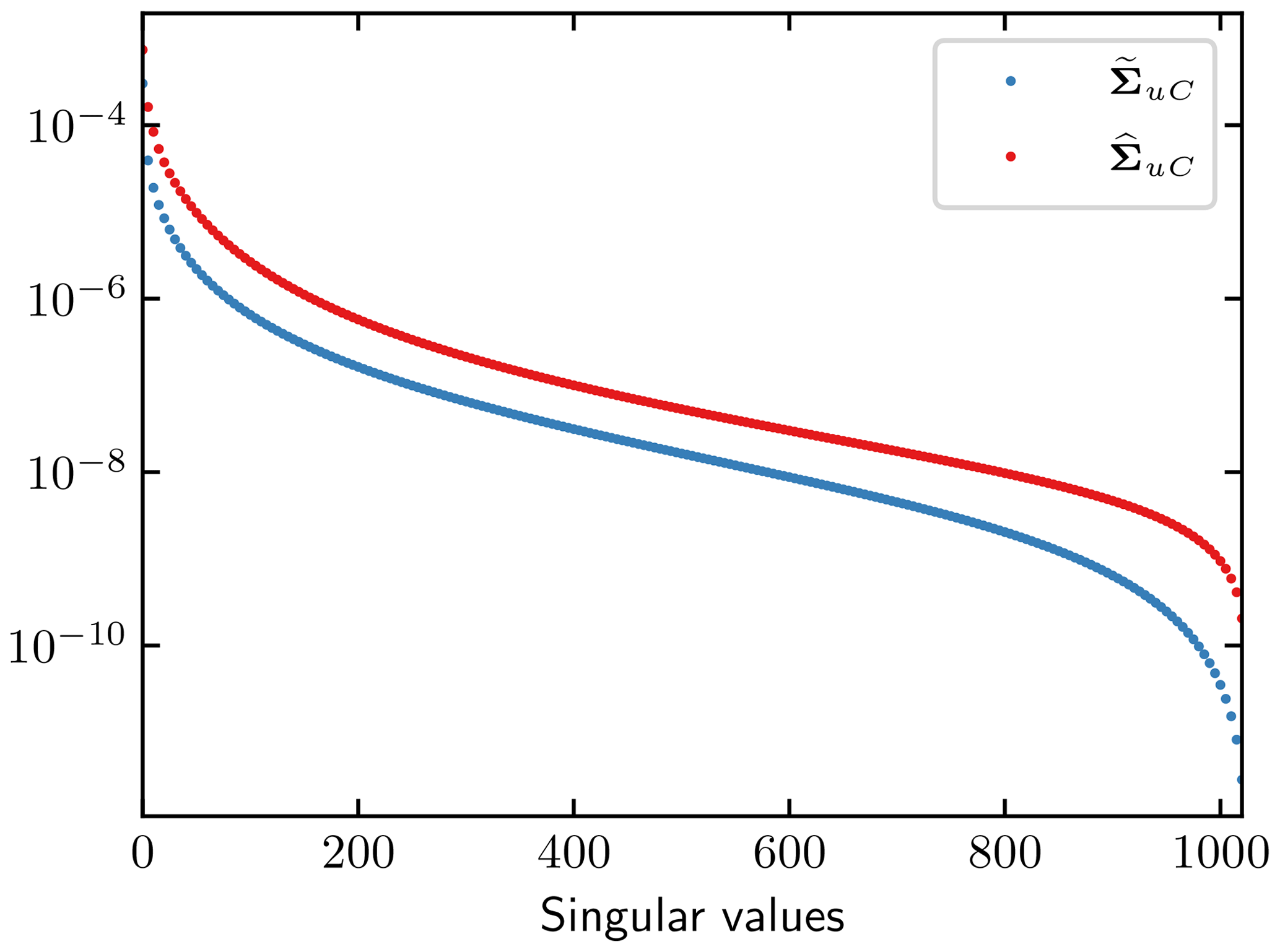
The singular values of the transfer matrices corresponding to the two simplifications are displayed in Fig. 15, where the two transfer matrices are denoted by for the system coupling ψ and v and by for the adjoint equation without ψ with a fixed H. The singular values in are similar to those in ΣuC in Fig. 9 since the influence of the adjoint viscosity on the system is almost negligible. The transfer matrix has a better conditioning than , although it is still worse than the best cases in Fig. 9. This implies that the inversion of steady-state SSA without the height coupling may be an ill-posed problem. Regularization is necessary for penalizing oscillatory behavior at the base as in Gagliardini et al. (2013) and Petra et al. (2012).
A few issues are discussed here related to the control method for estimating the parameter sensitivity.
We solve the FS adjoint problem only one step backward in time to verify the numerical method due to limitations of the current framework of Elmer/Ice. It is possible but more complicated and expensive to solve the adjoint problem numerically for a large number of time steps K. This requires storing all the forward solutions to be able to compute the adjoint solutions which may be prohibitive in 3-D. Since the data to be stored in the SSA model are one dimension lower, we are able to solve the adjoint problem backward in time for any number of K. For a fair comparison, we show the results for one time step with SSA in this paper.
The equations for the adjoints of FS and SSA in Eqs. (8) and (15) are generally valid for an ice sheet in 3-D and have to be solved numerically. The problem with the storage of the forward solution is the same as in adaptive mesh refinement, where the time step and the mesh are adapted to satisfy bounds on the numerical error. Selected forward solutions in time are saved for the adjoint solution to reduce the storage requirements. Missing values are interpolated in time and the sensitivity integral in Eqs. (10) and (16) is computed successively when the adjoint solution is advanced backward in time.
The solutions of the horizontal velocity u and the height h with perturbations in C in the transient FS and SSA models are similar in Figs. 4 and 10. The weights in the upper panels in Figs. 2 and 6 are similar, too. The solutions to the forward equations are also close in the chosen MISMIP configuration. The reason is that the sliding on the ground in the FS model is considerable, making SSA a good approximation of FS.
There are many discussions regarding the choice of friction laws (see, e.g., Gladstone et al., 2017; Tsai et al., 2015; Brondex et al., 2017). However, assuming a spatial variability of the friction coefficient C(x) with a linear relation between the basal stress and velocity makes this numerical study independent of the friction law. The friction coefficient can be viewed as a linearization of the friction law, and a postprocessing procedure can retrieve the corresponding friction law.
The transfer relation WuC between small perturbations of the friction coefficient C at the ice base and the perturbation of the horizontal velocity u at the ice surface is given by Eq. (23) with δb=0. The singular values of WuC in Fig. 9 tell how sensitive u is to changes in C. The transfer relation also describes how the uncertainty in C is propagated to uncertainty in the velocity at the surface and how uncertainty δu in measurements of u appears as uncertainty δC in C Eq. (26); see Smith (2014).
The transfer relation is computed by solving the forward problem once and then the adjoint problem for each one of the M observations. An alternative would be to solve the forward equations first for the unperturbed solution and then perturb C by δCj and solve the forward equations again N times and subtract to find the relation between δu and δCj. It is usually more expensive to solve the nonlinear forward equations than the linear adjoint equations. Suppose that the computational work to solve the forward problem is 𝒲F and the adjoint problem is 𝒲A. If the forward and adjoint equations are in similar form, such as the FS or SSA problem, and solving the nonlinear forward problem requires k iterations, where every nonlinear iteration has the same computational cost as solving the linear adjoint problem, then . The quotient between the work to determine the transfer relation involving the adjoint equations and the work only based on the forward equation is . Since k≥1, it is advantageous to choose the approach involving the adjoint if M<kN. Otherwise, solve N+1 forward problems to compute WuC. In the inverse problem to find C given observations of u,h, the functions Fu and Fh are smooth and M=1 in the iterative procedure to compute C with a gradient method. Solving the adjoint equations is then always favorable.
The perturbations δu and δh in the velocity u and the height h at the ice surface are caused by perturbations δb and δC in the topography of the ice base b and the basal friction coefficient C. The sensitivities δu and δh to δb and δC are evaluated in 2-D by first solving the adjoint equations of the FS and SSA models including the advection equation for the height derived in Cheng and Lötstedt (2019). Then weight or transfer functions are determined for the relation between δu and δh at the surface and δb and δC at the base. The predictions of δu and δh with the weights are compared to explicit calculations of perturbed u and h at the surface with good agreement. It is shown in Cheng and Lötstedt (2019) that if the base perturbations are time dependent then it is necessary to have time-dependent weight functions to obtain the correct behavior at the top of the ice.
Both the height and the stress equations and their adjoints are solved to find the weight functions here. The inverse problem at steady state to infer C from observations of u is usually solved for a fixed ice geometry and with only the stress equation and its adjoint (see, e.g., MacAyeal, 1993; Petra et al., 2012). This is possible since the adjoint height ψ is small when the horizontal part of u is observed and has little influence on δu. On the contrary, if h is observed then there is an important effect of ψ on δh in FS and SSA. The magnitudes of ψ are different depending on whether u or h is observed. Simplifications of the SSA adjoint in the steady state by using the forward viscosity or ignoring the adjoint height equation have minor consequences for the predictions of u with a perturbed C in Fig. 14.
The sensitivity to perturbations δb and δC is quantified for steady-state and time-dependent problems with the FS and SSA models. It increases as the observation point x∗ approaches the grounding line. This is explained by analytical expressions for SSA where the sensitivity is proportional to the velocity u and inversely proportional to the ice thickness H(x∗). The closer we are to the grounding line the higher the requirements are on the resolution of the topography and the friction coefficient to obtain accurate solutions of u and h there. This is observed numerically in Durand et al. (2011).
A weight is local if its extension in space is close to the observation point. The weights on δC at the ice base are local for the steady-state and time-dependent FS model. They are also local for the time-dependent SSA model and the transfer from δb to δu and δh in the steady state. The sensitivity of δu and δh in the steady state of SSA depends on δC from a larger domain. It is difficult to observe a perturbation δC with a short wavelength on u and h. In the example in Fig. 3, a spatial perturbation wavelength m (about 10H) in C is damped by 0.2 in δh and 0.02 in δu compared to a wavelength λ>105 where there is no damping due to λ. This is in agreement with the theory in Gudmundsson (2008).
The perturbations in u and h in the steady state of the SSA model consist of a direct effect from δb at the observation point and a nonlocal effect of δb and δC in Figs. 6 and 7. It follows from the analytical solution in Eq. (A3) that we cannot distinguish between the nonlocal contributions of δb and δC in the integral to δu. The same conclusion about the nonlocal perturbations holds for δh in Eq. (A5). This is also an observation in Kyrke-Smith et al. (2018).
The transfer matrices from δb and δC to δu and δh are examined by the singular value decomposition. If the quotient between the largest and the smallest singular values of the matrix is large then it is ill-conditioned, and if it is small (but ≥1) then the problem is well-conditioned. In an ill-conditioned problem, some perturbations at the base will be barely visible at the surface, and a small perturbation at the top may correspond to a large perturbation at the bottom. In a well-conditioned problem, all perturbations at the base have a measurable effect at the surface. The ranking of the conditioning of the transfers in Fig. 9 from the best to the worst is
In the past, the coupling between δu and δC is most frequently used for inference of C from velocity data, but adding height data would improve the robustness of the inference. The approximated analytical transfer functions for SSA, yielding explicit dependence of the parameters, have the same properties as above in which the observed velocity u and height h are more sensitive to perturbations δb than δC.
Detailed derivations of the formulas are found in Cheng and Lötstedt (2019). A variable with index ∗ is evaluated at x∗.
A1 The forward steady-state SSA solution
The analytical steady-state solution to the forward Eq. (17) without considering the viscosity terms is
where HGL is the thickness of the ice at the grounding line xGL.
A2 The adjoint steady-state SSA solutions
The analytical steady-state solutions of the SSA adjoint Eq. (18) with observation of u at x∗ are
where H∗ is the thickness of the ice at x∗. The corresponding perturbation δu∗ in Eq. (20) has the weights for δC and δb as
If h is observed at x∗, then
The weights for δC and δb in Eq. (19) for the perturbation on h∗ are
A3 The singular value decomposition (SVD)
The SVD factorizes a matrix A in the following way (see Golub and Van Loan, 1989):
If A is an M×N matrix then U is an M×M matrix, Σ an M×N matrix, and V an N×N matrix. The singular values σi are nonnegative and ordered from large to small for increasing i and . They form the diagonal of the diagonal matrix Σ with Σii=σi. The other two matrices are orthogonal, satisfying UTU=I and VTV=I. The generalized inverse Σ−1 of Σ is an N×M matrix with (if σi is positive) on the diagonal and 0 elsewhere.
The FS equations are solved using Elmer/Ice version 8.4 (rev. f6bfdc9) with the scripts at: https://doi.org/10.5281/zenodo.3611158 (Cheng, 2020a). The forward and adjoint SSA solvers are implemented in MATLAB. The code is available at: https://doi.org/10.5281/zenodo.3611154 (Cheng, 2020b).
GC contributed most of the computations, and GC and PL contributed equally to the theory and the writing of the paper.
The authors declare that they have no conflict of interest.
Thomas Zwinger helped with the adjoint FS solver in Elmer/Ice. Comments by Lina von Sydow helped us improve a draft of the paper, and Murtazo Nazarov explained the algorithm for adaptive mesh refinement.
This research has been supported by a Svenska Forskningsrådet Formas grant (no. 2017-00665) to Nina Kirchner and the Swedish strategic research program eSSENCE.
This paper was edited by Alexander Robinson and reviewed by two anonymous referees.
Baiocchi, C., Brezzi, F., and Franca, L. P.: Virtual bubbles and Galerkin-least-squares type methods (Ga. LS), Comp. Meth. Appl. Mech. Eng., 105, 125–141, 1993. a
Brondex, J., Gagliardini, O., Gillet-Chaulet, F., and Durand, G.: Sensitivity of grounding line dynamics to the choice of the friction law, J. Glaciol., 63, 854–866, 2017. a
Bulthuis, K., Arnst, M., Sun, S., and Pattyn, F.: Uncertainty quantification of the multi-centennial response of the Antarctic ice sheet to climate change, The Cryosphere, 13, 1349–1380, https://doi.org/10.5194/tc-13-1349-2019, 2019. a
Cheng, G.: Numerical experiments for FS adjoint, Zenodo, https://doi.org/10.5281/zenodo.3611158, 2020a. a
Cheng, G.: Numerical experiments for SSA adjoint, Zenodo, https://doi.org/10.5281/zenodo.3611154, 2020b. a
Cheng, G. and Lötstedt, P.: Parameter sensitivity analysis of dynamic ice sheet models, Tech. Rep., arXiv:1906.08197, 2019. a, b, c, d, e, f, g, h, i, j, k, l
Durand, G., Gagliardini, O., Favier, L., Zwinger, T., and Le Meur, E.: Impact of bedrock description on modeling ice sheet dynamics, Geophys. Res. Lett., 38, L20501, https://doi.org/10.1029/2011GL048892, 2011. a, b
Gagliardini, O., Zwinger, T., Gillet-Chaulet, F., Durand, G., Favier, L., de Fleurian, B., Greve, R., Malinen, M., Martín, C., Råback, P., Ruokolainen, J., Sacchettini, M., Schäfer, M., Seddik, H., and Thies, J.: Capabilities and performance of Elmer/Ice, a new-generation ice sheet model, Geosci. Model Dev., 6, 1299–1318, https://doi.org/10.5194/gmd-6-1299-2013, 2013. a, b, c, d
Gillet-Chaulet, F., Gagliardini, O., Seddik, H., Nodet, M., Durand, G., Ritz, C., Zwinger, T., Greve, R., and Vaughan, D. G.: Greenland ice sheet contribution to sea-level rise from a new-generation ice-sheet model, The Cryosphere, 6, 1561–1576, https://doi.org/10.5194/tc-6-1561-2012, 2012. a
Gillet-Chaulet, F., Durand, G., Gagliardini, O., Mosbeux, C., Mouginot, J., Rémy, F., and Ritz, C.: Assimilation of surface velocities acquired between 1996 and 2010 to constrain the form of the basal friction law under Pine Island Glacier, Geophys. Res. Lett., 43, 10311–10321, 2016. a, b
Gladstone, R. M., Warner, R. C., Galton-Fenzi, B. K., Gagliardini, O., Zwinger, T., and Greve, R.: Marine ice sheet model performance depends on basal sliding physics and sub-shelf melting, The Cryosphere, 11, 319–329, https://doi.org/10.5194/tc-11-319-2017, 2017. a
Goldberg, D., Heimbach, P., Joughin, I., and Smith, B.: Committed retreat of Smith, Pope, and Kohler Glaciers over the next 30 years inferred by transient model calibration, The Cryosphere, 9, 2429–2446, https://doi.org/10.5194/tc-9-2429-2015, 2015. a
Golub, G. H. and Van Loan, C. F.: Matrix Computations, Johns Hopkins University Press, Baltimore, 2nd edn., 1989. a, b, c
Greve, R. and Blatter, H.: Dynamics of Ice Sheets and Glaciers, Advances in Geophysical and Environmental Mechanics and Mathematics (AGEM2), Springer, Berlin, 2009. a, b, c, d
Gudmundsson, G. H.: Transmission of basal variability to glacier surface, J. Geophys. Res., 108, 2253, https://doi.org/10.1029/2002JB002107, 2003. a, b, c, d
Gudmundsson, G. H.: Analytical solutions for the surface response to small amplitude perturbations in boundary data in the shallow-ice-stream approximation, The Cryosphere, 2, 77–93, https://doi.org/10.5194/tc-2-77-2008, 2008. a, b, c, d, e, f
Isaac, T., Petra, N., Stadler, G., and Ghattas, O.: Scalable and efficient algorithms for the propagation of uncertainty from data through inference to prediction for large-scale problems with application to flow of the Antarctic ice sheet, J. Comput. Phys., 296, 348–368, 2015. a, b
Jay-Allemand, M., Gillet-Chaulet, F., Gagliardini, O., and Nodet, M.: Investigating changes in basal conditions of Variegated Glacier prior to and during its 1982–1983 surge, The Cryosphere, 5, 659–672, https://doi.org/10.5194/tc-5-659-2011, 2011. a
Kyrke-Smith, T. M., Gudmundsson, G. H., and Farrell, P. E.: Relevance of detail in basal topography for basal slipperiness inversions: a case study on Pine Island Glacier, Antarctica, Frontiers Earth Sci., 6, 33, https://doi.org/10.3389/feart.2018.00033, 2018. a, b, c, d, e
Larour, E., Utke, J., Csatho, B., Schenk, A., Seroussi, H., Morlighem, M., Rignot, E., Schlegel, N., and Khazendar, A.: Inferred basal friction and surface mass balance of the Northeast Greenland Ice Stream using data assimilation of ICESat (Ice Cloud and land Elevation Satellite) surface altimetry and ISSM (Ice Sheet System Model), The Cryosphere, 8, 2335–2351, https://doi.org/10.5194/tc-8-2335-2014, 2014. a
Leguy, G. R., Asay-Davis, X. S., and Lipscomb, W. H.: Parameterization of basal friction near grounding lines in a one-dimensional ice sheet model, The Cryosphere, 8, 1239–1259, https://doi.org/10.5194/tc-8-1239-2014, 2014. a
MacAyeal, D. R.: Large-scale ice flow over a viscous basal sediment: Theory and application to Ice Stream B, Antarctica, J. Geophys. Res., 94, 4071–4078, 1989. a, b
MacAyeal, D. R.: A tutorial on the use of control methods in ice sheet modeling, J. Glaciol., 39, 91–98, 1993. a, b, c, d
Martin, N. and Monnier, J.: Adjoint accuracy for the full Stokes ice flow model: limits to the transmission of basal friction variability to the surface, The Cryosphere, 8, 721–741, https://doi.org/10.5194/tc-8-721-2014, 2014. a
Monnier, J. and des Boscs, P.-E.: Inference of the bottom properties in shallow ice approximation models, Inverse Problems, 33, 115001, https://doi.org/10.1088/1361-6420/aa7b92, 2017. a
Morlighem, M., Seroussi, H., Larour, E., and Rignot, E.: Inversion of basal friction in Antarctica using exact and incomplete adjoints of a high-order model, J. Geophys. Res.-Earth Surf., 118, 1–8, 2013. a
Mosbeux, C., Gillet-Chaulet, F., and Gagliardini, O.: Comparison of adjoint and nudging methods to initialise ice sheet model basal conditions, Geosci. Model Dev., 9, 2549–2562, https://doi.org/10.5194/gmd-9-2549-2016, 2016. a
Pattyn, F., Schoof, C., Perichon, L., Hindmarsh, R. C. A., Bueler, E., de Fleurian, B., Durand, G., Gagliardini, O., Gladstone, R., Goldberg, D., Gudmundsson, G. H., Huybrechts, P., Lee, V., Nick, F. M., Payne, A. J., Pollard, D., Rybak, O., Saito, F., and Vieli, A.: Results of the Marine Ice Sheet Model Intercomparison Project, MISMIP, The Cryosphere, 6, 573–588, https://doi.org/10.5194/tc-6-573-2012, 2012. a, b
Petra, N., Zhu, H., Stadler, G., Hughes, T. J. R., and Ghattas, O.: An inexact Gauss-Newton method for inversion of basal sliding and rheology parameters in a nonlinear Stokes ice sheet model, J. Glaciol., 58, 889–903, 2012. a, b, c, d, e, f, g, h
Schannwell, C., Drews, R., Ehlers, T. A., Eisen, O., Mayer, C., and Gillet-Chaulet, F.: Kinematic response of ice-rise divides to changes in ocean and atmosphere forcing, The Cryosphere, 13, 2673–2691, https://doi.org/10.5194/tc-13-2673-2019, 2019. a
Schlegel, N.-J., Seroussi, H., Schodlok, M. P., Larour, E. Y., Boening, C., Limonadi, D., Watkins, M. M., Morlighem, M., and van den Broeke, M. R.: Exploration of Antarctic Ice Sheet 100-year contribution to sea level rise and associated model uncertainties using the ISSM framework, The Cryosphere, 12, 3511–3534, https://doi.org/10.5194/tc-12-3511-2018, 2018. a
Schoof, C.: Ice-sheet acceleration driven by melt supply variability, Nature, 468, 803–806, 2010. a, b
Seddik, H., Greve, R., Sakakibara, D., Tsutaki, S., Minowa, M., and Sugiyama, S.: Response of the flow dynamics of Bowdoin Glacier, northwestern Greenland, to basal lubrication and tidal forcing, J. Glaciol., 65, 225–238, https://doi.org/10.1017/jog.2018.106, 2019. a
Sergienko, O. and Hindmarsh, R. C. A.: Regular patterns in frictional resistance of ice-stream beds seen by surface data inversion, Science, 342, 1086–1089, 2013. a
Shannon, S. R., Payne, A. J., Bartholomew, I. D., van den Broeke, M. R., Edwards, T. L., Fettweis, X., Gagliardini, O., Gillet-Chaulet, F., Goelzer, H., Hoffman, M. J., Huybrechts, P., Mair, D. W. F., Nienow, P. W., Perego, M., Price, S. F., Smeets, C. J. P. P., Sole, A. J., van de Wal, R. S. W., and Zwinger, T.: Enhanced basal lubrication and the contribution of the Greenland ice sheet to future sea–level rise, P. Natl. Acad. Sci. USA, 110, 14156–14161, 2013. a, b
Smith, R. C.: Uncertainty Quantification. Theory, Implementation, and Applications, Society for Industrial and Applied Mathematics, Philadelphia, 2014. a, b
Sole, A. J., Mair, D. W. F., Nienow, P. W., Bartholomew, I. D., King, I. D., Burke, M. A., and Joughin, I.: Seasonal speedup of a Greenland marine-terminating outlet glacier forced by surface melt-induced changes in subglacial hydrology, J. Geophys. Res., 116, F03014, https://doi.org/10.1029/2010JF001948, 2011. a
Sun, S., Cornford, S. L., Liu, Y., and Moore, J. C.: Dynamic response of Antarctic ice shelves to bedrock uncertainty, The Cryosphere, 8, 1561–1576, https://doi.org/10.5194/tc-8-1561-2014, 2014. a
Tsai, V. C., Stewart, A. L., and Thompson, A. F.: Marine ice-sheet profiles and stability under Coulomb basal conditions, J. Glaciol., 61, 205–215, 2015. a
Vallot, D., Pettersson, R., Luckman, A., Benn, D. I., Zwinger, T., van Pelt, W. J. J., Kohler, J., Schäfer, M., Claremar, B., and Hulton, N. R. J.: Basal dynamics of Kronebreen, a fast-flowing tidewater glacier in Svalbard: non-local spatio-temporal response to water input, J. Glaciol., 11, 179–190, 2017. a
van Pelt, W. J. J., Oerlemans, J., Reijmer, C. H., Pettersson, R., Pohjola, V. A., Isaksson, E., and Divine, D.: An iterative inverse method to estimate basal topography and initialize ice flow models, The Cryosphere, 7, 987–1006, https://doi.org/10.5194/tc-7-987-2013, 2013. a, b
Weertman, J.: On the sliding of glaciers, J. Glaciol., 3, 33–38, 1957. a