the Creative Commons Attribution 4.0 License.
the Creative Commons Attribution 4.0 License.
 | 14 Feb 2020
Glacial-cycle simulations of the Antarctic Ice Sheet with the Parallel Ice Sheet Model (PISM) – Part 2: Parameter ensemble analysis
Ricarda Winkelmann
Anders Levermann
The Parallel Ice Sheet Model (PISM) is applied to the Antarctic Ice Sheet over the last two glacial cycles (≈210 000 years) with a resolution of 16 km. An ensemble of 256 model runs is analyzed in which four relevant model parameters have been systematically varied using full-factorial parameter sampling. Parameters and plausible parameter ranges have been identified in a companion paper (Albrecht et al., 2020) and are associated with ice dynamics, climatic forcing, basal sliding and bed deformation and represent distinct classes of model uncertainties. The model is scored against both modern and geologic data, including reconstructed grounding-line locations, elevation–age data, ice thickness, surface velocities and uplift rates. An aggregated score is computed for each ensemble member that measures the overall model–data misfit, including measurement uncertainty in terms of a Gaussian error model (Briggs and Tarasov, 2013). The statistical method used to analyze the ensemble simulation results follows closely the simple averaging method described in Pollard et al. (2016).
This analysis reveals clusters of best-fit parameter combinations, and hence a likely range of relevant model and boundary parameters, rather than individual best-fit parameters. The ensemble of reconstructed histories of Antarctic Ice Sheet volumes provides a score-weighted likely range of sea-level contributions since the Last Glacial Maximum (LGM) of 9.4±4.1 m (or ), which is at the upper range of most previous studies. The last deglaciation occurs in all ensemble simulations after around 12 000 years before present and hence after the meltwater pulse 1A (MWP1a). Our ensemble analysis also provides an estimate of parametric uncertainty bounds for the present-day state that can be used for PISM projections of future sea-level contributions from the Antarctic Ice Sheet.
- Article
(9946 KB) - Full-text XML
- Companion paper
-
Supplement
(4507 KB) - BibTeX
- EndNote


Sea-level estimates involve high uncertainty, in particular with regard to the potential instability of marine-based parts of the Antarctic Ice Sheet (e.g., Weertman, 1974; Mercer, 1978; Slangen et al., 2017). Processed-based models provide the tools to evaluate the currently observed ice sheet changes (Shepherd et al., 2018a, b); to better distinguish between natural drift, variability and anthropogenic drivers (Jenkins et al., 2018); and to estimate future changes for possible climatic boundary conditions (Oppenheimer and Alley, 2016; Shepherd and Nowicki, 2017; Pattyn, 2018). Regarding the involved variety of uncertain parameters and boundary conditions, confidence of future projections from such models is strengthened by systematic validation against modern observations and past reconstructions. We can build on experience gained in several preceding Antarctic modeling studies (Briggs et al., 2013, 2014; Whitehouse et al., 2012a; Golledge et al., 2014; Maris et al., 2014, 2015; Pollard et al., 2016, 2017; Quiquet et al., 2018), providing paleo-dataset compilations or advanced scoring schemes. Modern datasets encompass ice thickness, grounding-line and calving front position (Bedmap2; Fretwell et al., 2013), surface velocity (Rignot et al., 2011), and uplift rates from GPS measurements (Whitehouse et al., 2012b). Reconstructions of the grounding-line location at the Last Glacial Maximum (LGM) as provided by the RAISED consortium (Bentley et al., 2014) are used as paleo-constraints as well as grounding-line locations and cosmogenic elevation–age data from the AntICEdat database (Briggs and Tarasov, 2013) at specific sites during the deglaciation period.
In this study we run simulations of the entire Antarctic Ice Sheet with the Parallel Ice Sheet Model (PISM; Winkelmann et al., 2011; The PISM authors, 2020a, b). The hybrid of two shallow approximations of the stress balance and the comparably coarse resolution of 16 km allow for running an ensemble of simulations of ice sheet dynamics over the last two (dominant) glacial cycles, each lasting for about 100 000 years (or 100 kyr). The three-dimensional evolution of the enthalpy within the ice sheet accounts for the formation of temperate ice (Aschwanden and Blatter, 2009; Aschwanden et al., 2012) and for the production of subglacial water (Bueler and van Pelt, 2015). We use the non-conserving mode of the subglacial hydrology model, which balances the basal melt rate and constant drainage rate, to determine the effective pressure on the saturated till. The so-called till friction angle (accounting for small-scale till strength) and the effective pressure enter the Mohr–Coulomb yield stress criterion (Cuffey and Paterson, 2010). The yield criterion, in turn, is part of the pseudo-plastic sliding law, which relates basal sliding velocity to basal shear stress.
PISM comes with a computationally efficient generalization of the elastic-plate lithosphere with relaxing asthenosphere (ELRA) Earth model (Lingle and Clark, 1985; Bueler et al., 2007), with spatially varying flow in a viscous upper-mantle half-space below the elastic plate, which does not require relaxation time as a parameter. Geothermal heat flux based on airborne magnetic data from Martos et al. (2017) is applied to the lower boundary of a bedrock thermal layer of 2 km thickness, which accounts for storage effects of the upper lithosphere and hence estimates the heat flux at the ice–bedrock interface. Climate boundary conditions are based on mean precipitation from RACMO2.3p2 (van Wessem et al., 2018) and a temperature parameterization based on ERA-Interim reanalysis data (Simmons, 2006) in combination with the empirical positive-degree-day (PDD; e.g., Reeh, 1991) method. Climatic forcing is based on ice-core reconstructions from EPICA Dome C (EDC; Jouzel et al., 2007) and WAIS (West Antarctic Ice Sheet) Divide ice core (WDC; Cuffey et al., 2016) as well as on sea-level reconstructions from the ICE-6G GIA model (Stuhne and Peltier, 2015, 2017). Sub-shelf melting in PISM is calculated via PICO (Reese et al., 2018) from observed salinity and temperature in the lower ocean layers on the continental shelf adjacent to the ice shelves around the Antarctic continent (Schmidtko et al., 2014). Therein we consider mean values over 18 separate basins based on Zwally et al. (2015). PICO updates melt rates according to changes in ocean temperatures or the geometry of the ice shelves (while changes in salinity are neglected). A description of PISM for paleo-applications and sensitivity of the model to various uncertain parameter and boundary conditions are discussed in a companion paper (Albrecht et al., 2020).
Here, we explore uncertain model parameter ranges related to internal ice-model dynamics and boundary conditions (e.g. climatic forcing, bedrock deformation and basal till properties) and use the large-ensemble approach with full-factorial sampling for the statistical analysis, following Pollard et al. (2016). In view of the even larger ensemble by Briggs et al. (2014) with 31 varied parameters and over 3000 simulations, our ensemble with only four varied parameters and 256 simulations is of a rather intermediate size, but this allows for much finer model resolution. The analysis procedure yields an aggregated score for each ensemble simulation, which measures the misfit between a PISM simulation and nine equally weighted types of datasets. Each score can be associated with a probabilistic weight to compute the average envelope of the simulated Antarctic Ice Sheet and equivalent sea-level histories, hence providing data-constrained present-day states that can be used for projections with PISM.
Ice sheet model simulations generally imply uncertainties in used parameterizations and applied boundary conditions. In order to generate uncertainty estimates for reconstructions of the Antarctic Ice Sheet history and equivalent sea-level envelopes, we employ an ensemble analysis approach that uses full-factorial sampling, i.e., one run for every possible combination of parameter values. Here we closely follow the simple-averaging approach used in Pollard et al. (2016). This method yields reasonable results for an adequately resolved parameter space, as more advanced statistical techniques interpolate results between sparsely separated points in multi-dimensional parameter space. However, the full-factorial simple averaging method strongly limits the number of varied parameters for available computer resources such that only the most relevant parameters to each class of climatic and boundary conditions were pre-selected (see companion paper; Albrecht et al., 2020) to cover a representative range of model responses.
2.1 Ensemble parameters
We identified four relevant independent PISM ensemble parameters, with a prior range for each parameter capturing different uncertainties in ice flow dynamics, glacial climate, basal friction and bedrock deformation. The selected parameters passed the two following main criteria of (1) showing a relatively high sensitivity of the ice volume to parameter change while (2) arriving at a present-day state with tolerable anomaly to observations, which is not at all self-evident. The four parameters and the four values used in the ensemble analysis are as follows.
-
ESIA is the ice flow enhancement parameter of the stress balance in shallow ice approximation (SIA; Morland and Johnson, 1980; Winkelmann et al., 2011, Eq. 7). Ice deforms more easily in shear for increasing values of 1, 2, 4 and 7 (non-dimensional) within the Glen–Paterson–Budd–Lliboutry–Duval law. It connects strain rates and deviatoric stresses τ for ice softness A, which depends on both the liquid water fraction ω and temperature T (Aschwanden et al., 2012),
In all ensemble runs, we used, for the shallow shelf approximation (SSA) stress balance, an enhancement factor of 0.6 (see Sect. 2.1 in companion paper), which is relevant to ice-stream and ice shelf regions.
-
PPQ is the exponent q used in “pseudo-plastic” sliding law which relates bed-parallel basal shear stress τb to sliding velocity ub in the form
as calculated from the SSA of the stress balance (Bueler and Brown, 2009), for threshold speed u0, and yields stress τc. The sliding exponent hence covers uncertainties in basal friction. The values are 0.25, 0.5, 0.75 and 1.0 (non-dimensional).
-
PREC is the precipitation scaling factor fp according to temperature forcing ΔT motivated by the Clausius–Clapeyron relationship and data analysis (Frieler et al., 2015), which can be formulated as an exponential function (Ritz et al., 1996; Quiquet et al., 2012) as
For given present-day mean precipitation field P0, the factor fp captures uncertainty in the climatic mass balance, in particular for glacial periods. Values are 2 % K−1, 5 % K−1, 7 % K−1 and 10 % K−1.
-
VISC is the mantle viscosity that determines the characteristic response time of the linearly viscous half-space of the Earth to changing ice and adjacent ocean loads (Bueler et al., 2007, Eq. 1). It covers uncertainties within the Earth model for values of 0.1×10²¹, 0.5×10²¹, 2.5×10²¹ and 10×1021Pa s.
2.2 Misfit evaluation with respect to individual data types
With four varied parameters and each parameter taking four values, the ensemble requires 256 runs. For an easier comparison to previous model studies, results are analyzed using the simple averaging method (Pollard et al., 2016). It calculates an objective aggregate score for each ensemble member that measures the misfit of the model result to a suite of selected observational modern and geologic data. The inferred misfit score is based on a generic form of an observational error model, assuming a Gaussian error distribution with respect to any observation interpretation uncertainty (Briggs and Tarasov, 2013, Eq. 1).
The present-day ice sheet geometry (thickness and grounding-line position) provides the strongest spatial constraint of all data types and also offers a temporal constraint in the late Holocene. Gridded datasets are remapped to 16 km model resolution. Most of the present-day observational constraints closely follow the definitions in Pollard et al. (2016, Appendix B, Approach A) but are weighted with each grid cell's specific area with respect to stereographic projection. We added observed modern surface velocity as an additional constraint and expanded the analysis to the entire Antarctic Ice Sheet.
-
TOTE is the mean-square-error mismatch of present-day grounded areas to observations (Fretwell et al., 2013), assuming an uncertainty in the grounding-line location of 30 km, as in Pollard et al. (2016, Appendix B1). Mismatch is calculated relative to the continental domain that is defined here as an area with bed elevation above −2500 m.
-
TOTI is the mean-square-error mismatch of present-day floating ice shelf areas to observations (Fretwell et al., 2013), assuming an uncertainty in the grounding-line and calving front location of 30 km, according to Pollard et al. (2016, Appendix B2).
-
TOTDH is the mean-square-error model misfit of present-day state to observed ice thickness (Fretwell et al., 2013) with respect to an assumed observational uncertainty of 10 m and evaluated over the contemporary grounded region, close to Pollard et al. (2016, Appendix B3).
-
TOTGL is the mean-square-error misfit to observed grounding-line location for the modeled Antarctic grounded mask (ice rises excluded) using a two-dimensional distance field approximation (https://pythonhosted.org/scikit-fmm, last access: 9 February 2020). This method is different to the GL2D constraint used in Pollard et al. (2016, Appendix B5) and is only applied to the present-day grounding line around the whole Antarctic Ice Sheet according to Fretwell et al. (Bedmap2; 2013) while considering observational uncertainty of 30 km as in TOTI and TOTE above.
-
UPL is the mean-square-error model misfit to modern GPS-based uplift rates on rock outcrops at 35 individual sites using the compilation by Whitehouse et al. (2012b, Table S2) including individual observational uncertainty. Misfit is evaluated for the closest model grid point as in Pollard et al. (2016, Appendix B8), including intra-data-type weighting (Briggs and Tarasov, 2013, Sect. 4.3.1).
-
TOTVEL is the mean-square-error misfit in (grounded) surface ice speed compared to a remapped version of observational data by Rignot et al. (2011), including their provided grid-cell-wise standard deviation, bounded below by 1.5 m yr−1.
Paleo-data-type constraints are partly based on the AntICEdat compilation by Briggs and Tarasov (2013, Sect. 4.2), closely following their model–data misfit computation. Their compilation also includes records of regional sea-level change above present-day elevation (RSL), which was not considered in this study, as PISM lacks a self-consistent sea-level model to account for regional self-gravitational effect of the order of up to several meters, which can be similar to the magnitude of post-glacial uplift. According to Pollard et al. (2016, Appendix B4) we evaluate past and present grounding-line locations along four relevant ice shelf basins.
-
TROUGH is the mean-square-error misfit of the modeled grounding-line position along four transects through the Ross, Weddell and Amery basins and Pine Island Glacier at the Last Glacial Maximum (20 kyr BP) as compared to reconstructions by Bentley et al. (RAISED consortium; 2014, Scenario A) and those at present day compared to Fretwell et al. (Bedmap2; 2013), both remapped to the model grid. An uncertainty of 30 km in the location of the grounding line is assumed as in Pollard et al. (2016, Appendix B4) but as a mean over the two most confident dates and for all four mentioned troughs. In contrast to previous model calibrations, reconstructions of the grounding-line position at 15, 10 and 5 kyr BP have not been taken into account here, as they would favor simulations that reveal a rather slow and progressive grounding-line retreat through the Holocene in both the Ross and Ronne Ice Shelf, which has not necessarily been the case (Kingslake et al., 2018).
-
ELEV is the mean of the squared misfit of past (cosmogenic) surface elevation vs. age in the last 120 kyr based on model–data differences at 106 individual sites (distributed over 26 regions, weighted by inverse areal density; see Sect. 4.3.1 in Briggs and Tarasov, 2013). For each data point the smallest misfit to observations is computed for all past ice surface elevations (sampled every 1 kyr) of the 16 km model grid interpolated to the core location and datum as part of a thinning trend (Briggs and Tarasov, 2013, Sect. 4.2). A subset of these data has also been used in Maris et al. (2015) and Pollard et al. (2016, Appendix B7).
-
EXT is the mean of the squared misfit of observed ice extent at 27 locations around the entire Antarctic Ice Sheet in the last 28 kyr with dates for the onset of open marine conditions (OMCs) or grounding-line retreat (GLR). The modeled age is computed as the most recent transition from grounded to floating ice conditions considering the sea-level anomaly. The model output every 1 kyr is interpolated down to the core location and linearly interpolated to 100 yr temporal resolution, while weighting is not necessary here, as described in Briggs and Tarasov (2013, Sect. 4.2). A subset of these data has been also used in Maris et al. (2015).
2.3 Score aggregation
Each of the misfits above are first transformed into a normalized individual score for each data type i and each run j using the median over all misfits Mi,j for the 256 simulations. The procedure closely follows Approach (A) in Pollard et al. (2016, Sect. 2.4.1). Then the individual score Si,j is normalized according to the median to
As in Pollard et al. (2016) we also assume that each data type is of equal importance to the overall score, avoiding the inter-data-type weighting used by Briggs and Tarasov (2013) and Briggs et al. (2014), which would favor data types of higher spatio-temporal density. Hence the aggregated score for each run j is the product of the nine data-type-specific scores, according to the score definition by Pollard et al. (2016):
This implies that one simulation with perfect fit to eight data types, but one low individual score, yields a low aggregated score for this simulation and hence, for instance, low confidence for future applications.
3.1 Analysis of parameter ensemble
We ran the full ensemble of PISM simulations over the last glacial cycle. Figure 1 shows the aggregate scores Sj for each of the 256 ensemble members over the 4-D space spanned by the parameters ESIA, PPQ, PREC and VISC. Each individual sub-panel shows PPQ vs. VISC, and the sub-panels are arranged from left to right for varying PREC and bottom to top for varying ESIA. Scores are normalized by the best-score member, which equals a value of 1 here.
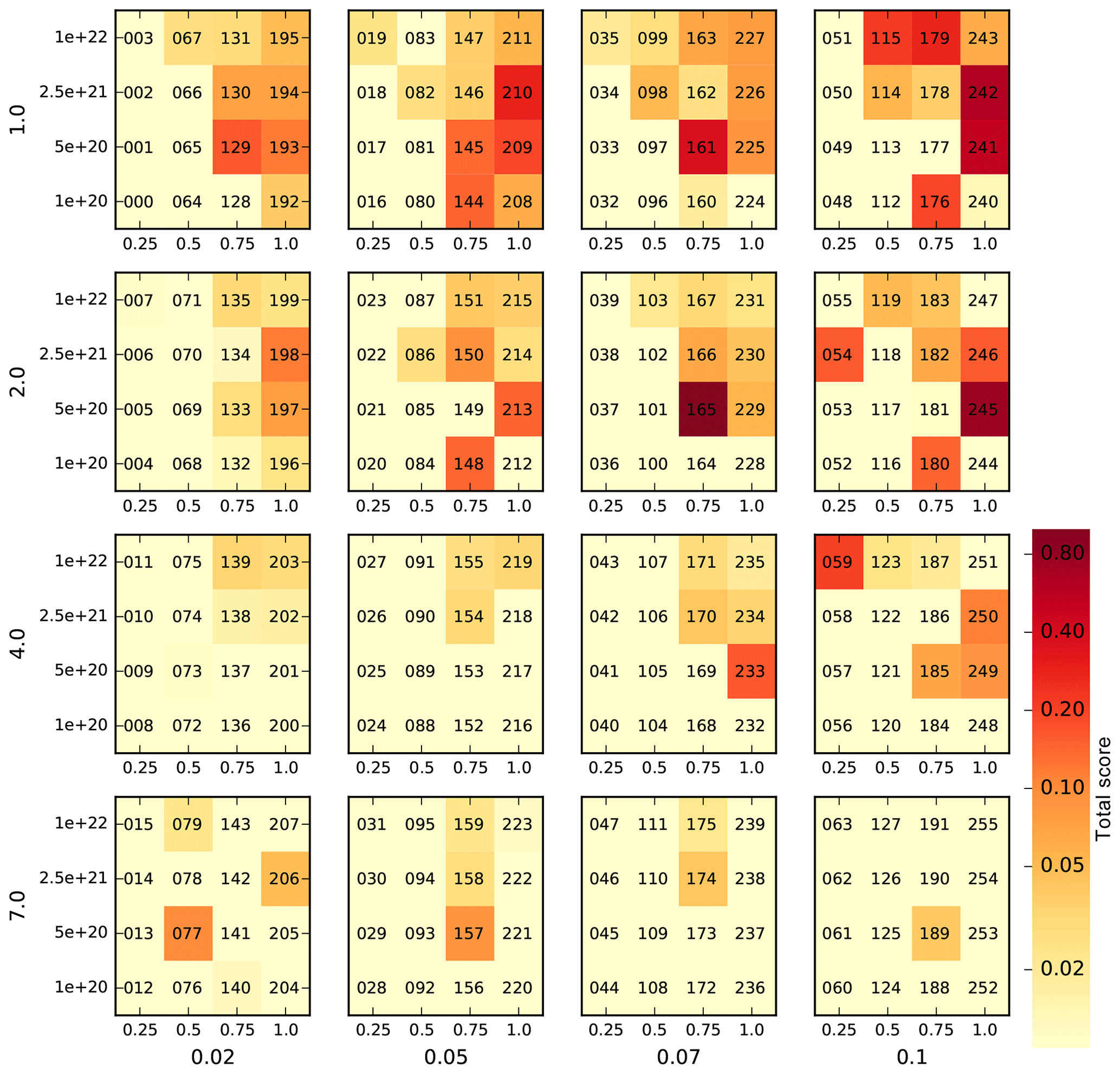
Figure 1Aggregated score for all 256 ensemble members (four model parameters; four values each), showing the distribution of the scores over the full range of plausible parameter values. The score values are computed versus geologic and modern datasets, normalized by the best score in the ensemble, and range from <0.01 (bright yellow – no skill) to 1.0 (dark red – best score) on a logarithmic color scale (cf. Pollard et al., 2016, Figs. 2 and C1). The four parameters are the SIA enhancement factor ESIA (outer y axis), the temperature-dependent precipitation scaling PREC (outer x axis), the mantle viscosity VISC (inner y axis) and the power-law sliding exponent PPQ (inner x axis).
The parameter ESIA enhances the shear-dominated ice flow and hence yields ice thinning, particularly in the interior of the ice sheet, and therewith a decrease in the total ice volume. ESIA values of 4.0 or 7.0 have been used in other models (e.g., Maris et al., 2015) to compensate for overestimated ice thickness in the interior of East Antarctic Ice Sheet under present-day climate conditions. In our ensemble, we find a trend towards higher scores for small ESIA values of 1.0 or 2.0 (in the top two rows of Fig. 1). This becomes more prominent when considering ensemble-mean score shares for individual parameter values as in Fig. 3, with a normalized mean score of 46 % for ESIA = 1.0 as compared to a mean score of 6 % for ESIA = 7.0. Most of this trend is a result of the individual data-type score TOTDH (see Fig. , column 4, row 3), as it measures the overall misfit of modern ice thickness (and volume distribution). Partly this trend can be also attributed to the TROUGH data-type scores (Fig. , column 8, row 3), as for higher ESIA values, grounding-line motion tends to slow down such that the time span between the LGM and present is not sufficient for a complete retreat back to the observed present-day location, at least in some ice shelf basins. The best-score ensemble members for small ESIA values are found in combination with both high values of mantle viscosity VISC and high values of the friction exponent PPQ (center-column panels in Fig. 4).
Regarding the choice of the precipitation scaling PREC the best-score members are found at the upper sampling range with values of 7 % K−1 or 10 % K−1 (see right two columns in Fig. 1). Considering the normalized ensemble-mean score for individual parameter values over the full range of 2 % K−1–10 % K−1, we can find a trend from 13 % to 42 % (see lowest panel in Fig. 3). Regarding parameter combinations with PREC (left-hand column in Fig. 4), we detect a weak trend towards lower ESIA and higher PPQ, while individual data-type scores (lower row in Fig. ) show a rather uniform pattern, in particular regarding the misfit to present-day observations. As the PREC parameter is linked to the temperature anomaly forcing, it affects the ice volume and hence the grounding-line location, particularly for temperature conditions different from present day. This suggests a stronger signal of PREC parameter variation in the paleo-data-type scores.
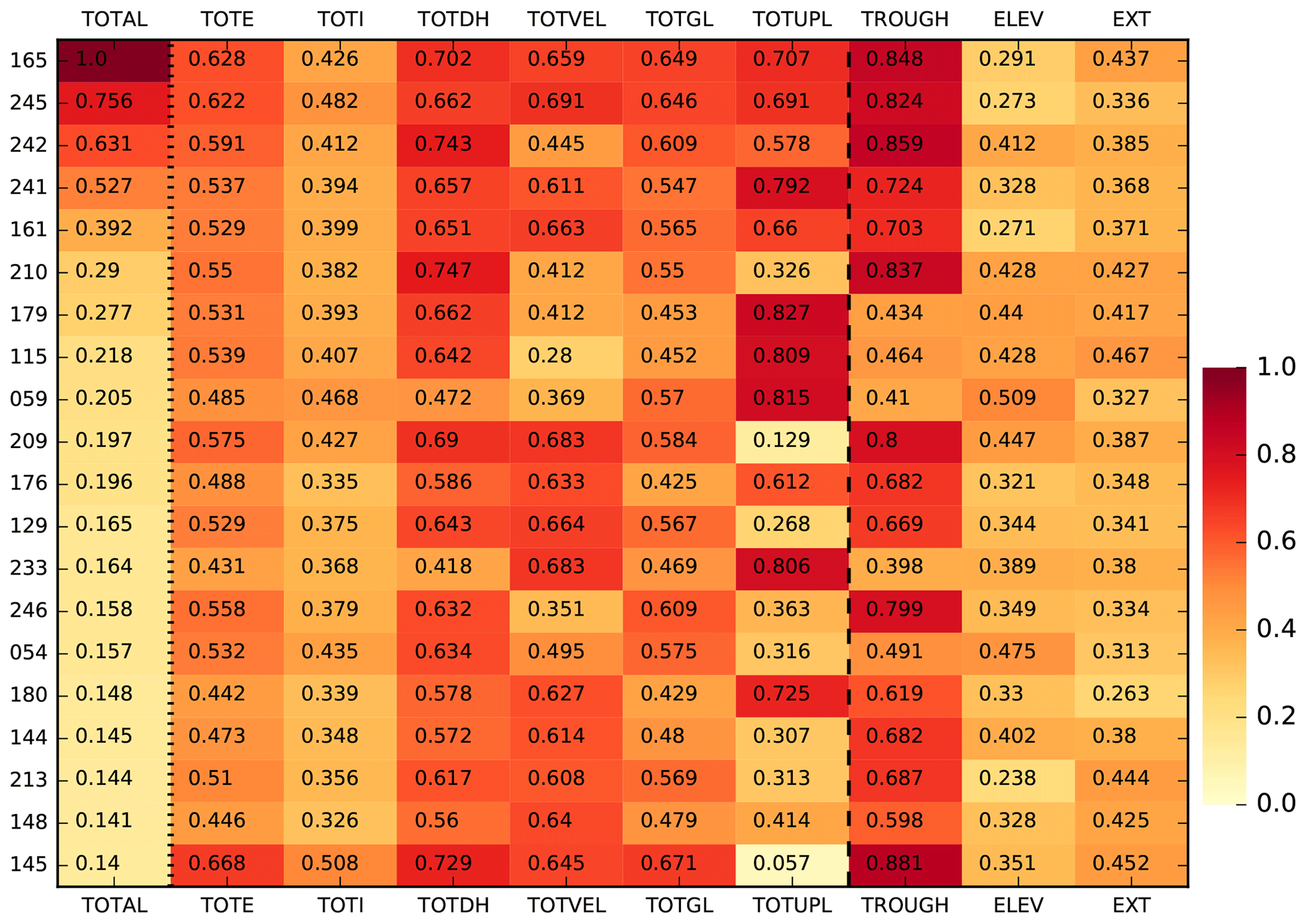
Figure 2Aggregated scores and nine individual scores for 20 best ensemble members computed versus modern and geologic datasets, divided by dashed line. The score values are normalized by the median misfit and range from 0 (bright yellow – no skill) to 1 (dark red – best score) on a linear color scale. The standard deviation for the individual paleo-data-type scores ELEV and EXT, as well as for present-day ice shelf mismatch TOTI, is below 0.1. In contrast, grounding-line location at LGM and present day along four ice shelf basins (TROUGH) and present-day uplift rates (TOTUPL) have the strongest impacts on the aggregated score, with a standard deviation of 0.2 and 0.3, respectively. Intermediate variability in individual scores show TOTGL, TOTE, TOTDH and TOTVEL with a standard deviation between 0.1 and 0.2.
A more complex pattern is found for PPQ in each of the sub-panels of Fig. 1, with the highest scores for values of 0.75 and 1.0. Averaged over the ensemble and normalized over the four parameter choices, we find a mean score of 5 % for PPQ = 0.25 (and hence rather plastic sliding), while the best scores are found for PPQ = 0.75 and PPQ = 1.0 (linear sliding), with mean scores of 40 % and 46 %, respectively (see second panel in Fig. 3). The best scores are found in combination with medium mantle viscosity VISC between 0.5×10²¹ and 2.5×10²¹ Pa s, as is visible in the upper right panel of Fig. 4. As sliding mainly affects the ice-stream flux, the trend in aggregated score over the range of PPQ values mainly results from the velocity misfit data-type TOTVEL and grounding-line-position-related data types (TOTE, TOTGL and THROUGH; see Fig. 3 – second row).
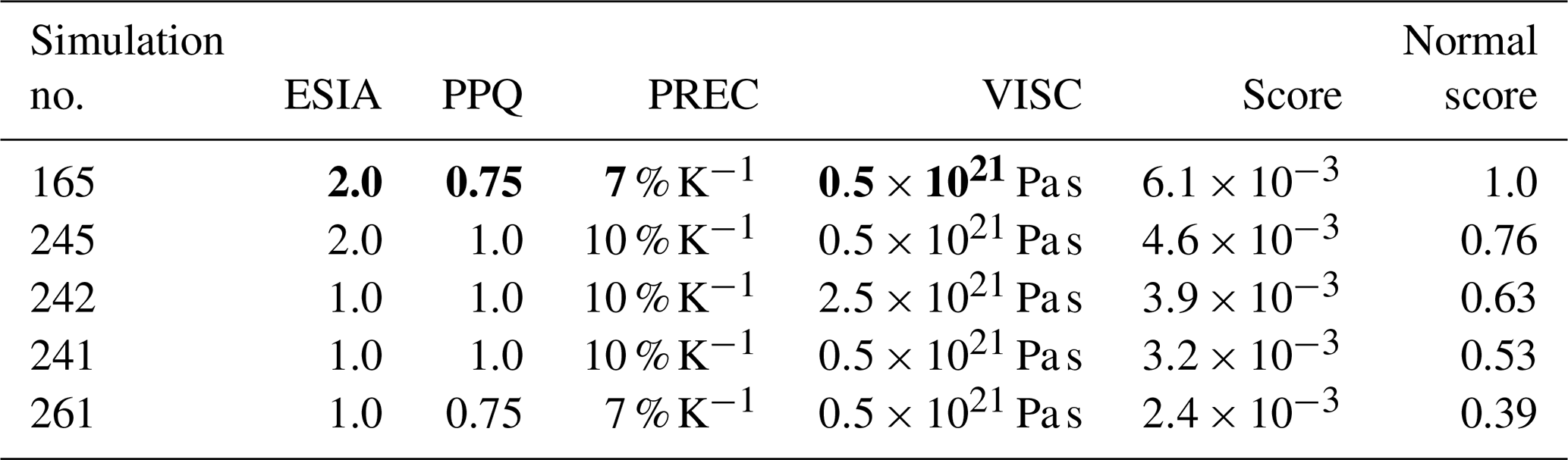
Table 1Five best-score ensemble parameter combinations with parameter values and total scores. The best-fit simulation parameters (bold) were used in the initMIP-Antarctica model intercomparison (PISMPAL3; Seroussi et al., 2019) and for the reference simulation in the companion paper (Albrecht et al., 2020).
Regarding mantle viscosity VISC, scores are generally low, at 9 % for the smallest sampled value of the parameter , while best scores are found in the ensemble for the 5-times-larger viscosity of Pa s, at 44 %. In our model, the mantle viscosity parameter has been applied to the whole Antarctic continent, although observations in some localized regions as in the Amundsen Sea suggest that upper-mantle viscosities could be considerably smaller than the tested range, up to the order of 1019 Pa s (Barletta et al., 2018). For the upper range of tested mantle viscosities, up to , we find a normalized ensemble mean of 27 % and 20 %, respectively. Note that VISC parameter values were sampled nonlinearly over a range of 2 orders of magnitude. For the lowest value there is a clear trend towards smaller scores in the grounding-line- and ice-thickness-related data types, such as TOTE, TOTGL, TROUGH and TOTDH. As mantle viscosity determines the rate of response of the bed to changes in ice thickness, a low viscosity corresponds to a rather quick uplift after grounding-line retreat and hence to a retarded retreat, which corresponds to a rather extended present-day state. This implies smaller ice shelves with slower flow and less velocity misfit such that also TOTVEL favors small VISC values. In contrast, a trend toward rather high mantle viscosities in the aggregated score stems mainly from the misfit of present-day uplift rates expressed as data-type score TOTUPL, probably due to reduced sensitivity to fluctuations in the grounding-line location. High mantle viscosities involve a slow bed uplift, and grounding-line retreat can occur faster. More specifically, in the partially overdeepened ice shelf basins, which were additionally depressed at the Last Glacial Maximum by a couple hundred meters as compared to present, grounding-line retreat can amplify itself in terms of regional marine ice sheet instability (Mercer, 1978; Schoof, 2007; Bart et al., 2016). In fact, the best-score ensemble members are found for intermediate mantle viscosities of and . This could be a result of the product formulation of the aggregated score, in which individual data-type scores favor opposing extreme values.
The five best-score ensemble members and associated parameter combinations are listed in Table 1. With the best-fit simulation parameters, we participated in the initMIP-Antarctica model intercomparison (PISMPAL3; Seroussi et al., 2019). The individual scores with respect to the nine data types are visualized for the 20 best ensemble members in Fig. 2. The scores associated with the paleo-data types ELEV and EXT show only comparably little variation among the ensemble (both around 0.07 standard deviation). This also applies for the present-day ice shelf area mismatch TOTI (0.04), as no calving parameter has been varied. In contrast, present-day data types associated with velocity (TOTVEL) and uplift rates (TOTUPL) show strong variations among the 20 best ensemble members, with a standard deviation in scores across the entire ensemble of 0.18 and 0.30, respectively. For data types that are related to grounding-line position (TOTGL, TOTE and TROUGH) and ice volume (TOTDH) we find a similar order as for the TOTAL aggregated score (Fig. 2), with individual standard deviations in scores of 0.12–0.20 across all ensemble members. All data-type-specific misfits are visualized as a histogram in the Supplement (Sect. B; Fig. S6).
Comparing the ensemble-mean present-day ice thickness with observations (Bedmap2; Fretwell et al., 2013) we find regions in the inner East Antarctic Ice Sheet and in parts of the Weddell Sea sector that are about 200 m too thin, while ice thickness is overestimated by more than 500 m on the Siple Coast, in the Amery basin and along the coastline, where smaller ice shelves tend to be grounded in the simulations (Fig. a). The Ross Sea, Weddell Sea and Amery basins show the largest ensemble-score-weighted standard deviation, with more than 500 m ice thickness (Fig. b). The ensemble spread in those basins can be associated with uncertainties in the grounding-line position. From its extended position at Last Glacial Maximum the grounding line has to retreat across the basins in time, with distances of up to 1000 km, leaving behind the large floating ice shelves (Fig. 6). In about 10 % of the score-weighted simulations, the grounding line remains at the extended position without significant retreat, linked to an efficient negative feedback on grounding-line motion, related to a fast-responding bed (low VISC). In contrast, for rather low friction and high mantle viscosities, we find fast grounding-line retreat, with a stabilization of the grounding-line position at or even inland of the observed location in 50 % or 75 % of the score-weighted simulations in the Ross and Weddell Sea sector, respectively (Fig. 7, upper panels). Due to the grounded ice retreat and the consequent unloading across the large ice shelf basins, the marine bed lifts up by up to a few hundred meters, which can lead to grounding line re-advance supported by the formation of ice rises (Kingslake et al., 2018). The ensemble-mean re-advance is up to 100 km, while some of the best-score simulations reveal temporary ungrounding through the Holocene up to 400 km upstream of the present-day grounding line in the Ross sector. The Amundsen Sea sector and Amery Ice Shelf do not show such rebound effects in our model ensemble (Fig. 7, lower panels).

Figure 3Ensemble-mean scores for individual parameter values (normalized such that sum is 1, or 100 %). The weighted mean over the four ensemble-mean scores with standard deviation is shown in red (compare Figs. 3 and C2 in Pollard et al., 2016).

Figure 4Ensemble-mean scores for six possible pairs of parameter values to visualize parameter dependency (compare Figs. 4 and C3 in Pollard et al., 2016). Values are normalized such that the sum for each pair is 1. Color scale is logarithmic, ranging from 0.01 (bright yellow) to 1 (red).
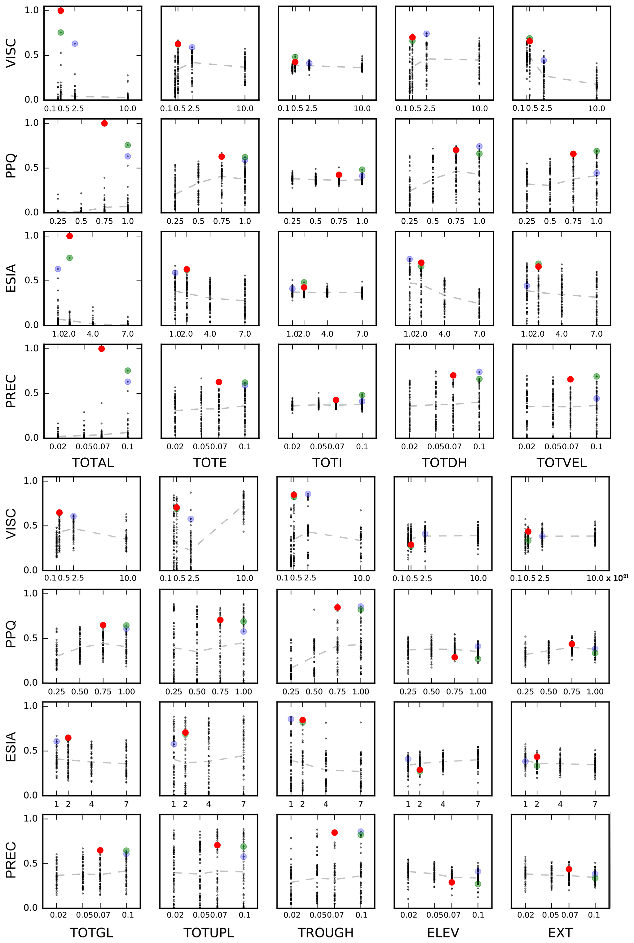
Figure 5Scatter plots of five individual data-type scores (panels from left to right; see definition in Sect. 2.2) for each parameter setting (VISC, PPQ, ESIA and PREC on y axis). Red dots indicate the best-score member; green and blue dots indicate the second and third best ensemble members (see Table 1). Grey dashed line indicates mean score tendency over sampled parameter range.
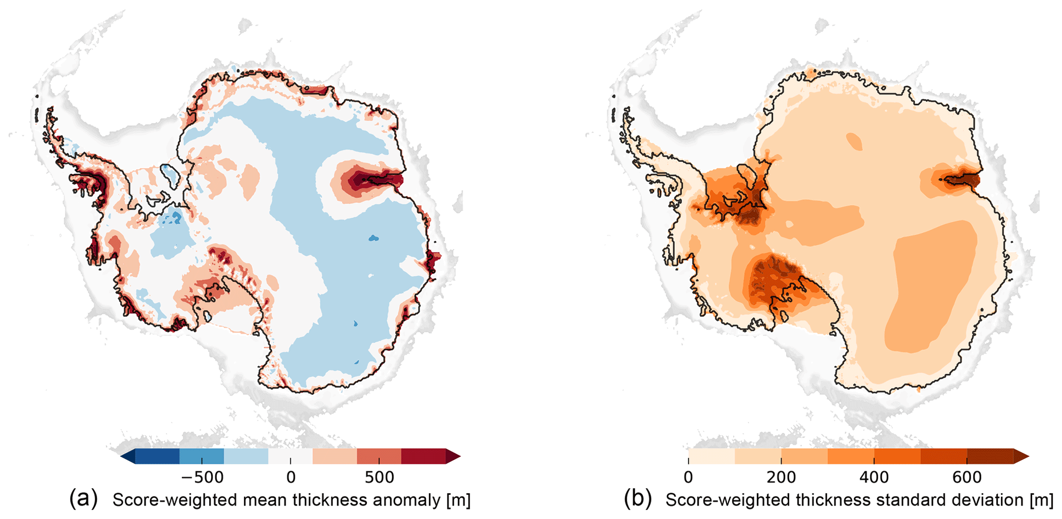
Figure 6Score-weighted mean ice thickness anomaly to Bedmap2 (a) and score-weighted standard deviation of ice thickness (b). Ice thickness in coastal regions in West Antarctica but also in the Amery basin are generally overestimated. Amery and Filchner–Ronne ice shelves and Siple Coast region reveal the highest standard deviation in reconstructed present-day ice thickness among the ensemble members.

Figure 7Ensemble-score-weighted grounded mask for 5 kyr snapshots. Mask value 1 (red) indicates grounded area which is covered by all simulations, while blueish colors indicate areas which are covered only by a few simulations with low scores (compare Fig. D4 in Pollard et al., 2016). For the last two snapshots, grounding line in the Ross Sea and Weddell Sea sector is found in about 50 % of score-weighted simulations inland of its present location (Fretwell et al., 2013, grey line), with some grounding-line re-advance (Kingslake et al., 2018; Siegert et al., 2019). In contrast less than 10 % of score-weighted simulations show no grounding-line retreat from glacial maximum extent. Black lines indicate reconstructions by the RAISED consortium (Bentley et al., 2014, Scenario B solid and scenario A dotted).
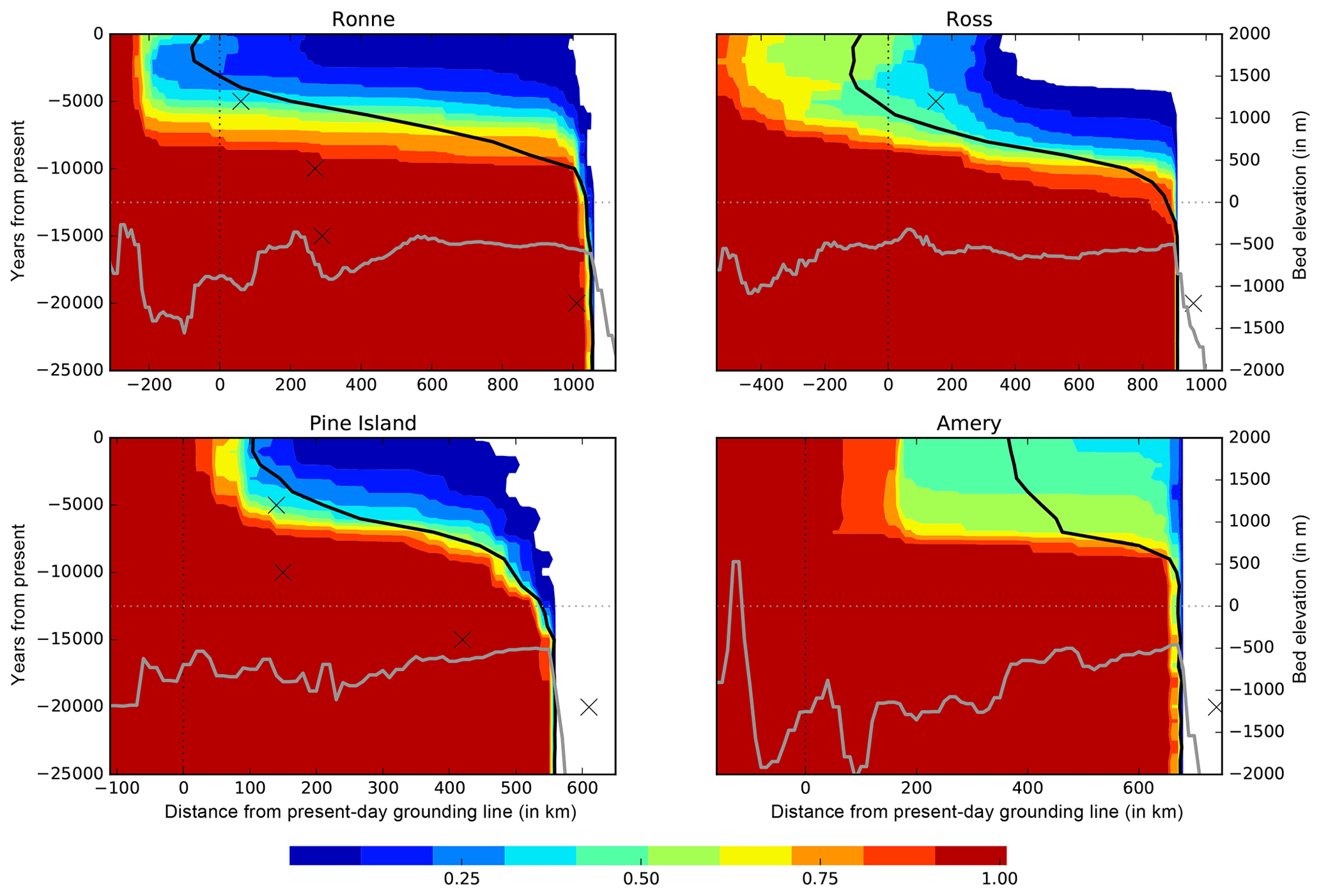
Figure 8Ensemble score-weighted grounded ice cover along transects trough Weddell, Ross, Amundsen and Amery Ice Shelf basins over the last 25 kyr simulation period (y axis in left panels; compare to Fig. D5 in Pollard et al., 2016). Grounded areas which are covered by all simulations are indicated by value 1 (red), while blueish colors indicate areas which are covered only by some simulations (or those with low scores). Grounding line in the Ross Sea and Weddell Sea sector is found inland of its present location (vertically dotted) within the last 10 kyr simulation time in about 50 % and 75 % of score-weighted simulations, respectively. The score-weighted mean curve (black) reveals re-advance of the grounding line of up to 100 km in about 20 % of the score-weighted simulations, both in the Ross and Weddell Sea sector, as discussed in Kingslake et al. (2018). Such behavior is not found in the Pine Island trough, where grounding-line retreat stops in 90 % of the simulations at about 200 km downstream of its present-day location. This is similar in the Amery Ice Shelf, where in 30 % of score-weighted simulations the ice shelf does not retreat at all from its LGM extent. Bed topography (Bedmap2; Fretwell et al., 2013) along the transect is indicated as grey line with respect to y axis in the right panels. For all four troughs, the data type TROUGH is evaluated for the two time slices, corresponding to LGM conditions (20 kyr BP; cross) and present day.
3.2 Reconstructed sea-level contribution histories
The full parameter ensemble is based on four simulations starting from the penultimate interglacial period (210 kyr BP). These four simulations use four different values of mantle viscosity covering 2 orders of magnitude (VISC = 1020−1022 Pa s). They show quite a consistent maximum ice volume at the penultimate glaciation around 130 kyr BP (see violet lines in Fig. 8). Due to the different Earth response times associated with varied mantle viscosities, the curves branch out when the ice sheet retreats. Those four simulations were used as initial states at 125 kyr BP for the other 252 simulations of the ensemble. At the end of the Last Interglacial (LIG) period (Eemian) at around 120 kyr BP, when the full ensemble was run for only 5 kyr, the ensemble-mean ice volume is 1.0 m SLE (meters of equivalent sea-level change) below modern levels, with a score-weighted standard deviation of around 2.7 m SLE (the volume of grounded ice above flotation in terms of “global mean sea-level equivalent” as defined in Albrecht et al., 2020; Sect. 1.2). This corresponds to a grounded ice volume anomaly in relation to present day observations of . These numbers may not reveal the full possible ensemble spread, as simulations still carry some memory of the previous glacial-cycle simulations with different parameters. On average, grounding lines and calving fronts retreat much further inland at LIG than for present-day conditions. However, complete collapse of the WAIS does not occur in any of the ensemble members, most likely as a result of intermediate till friction angles and hence higher basal shear stress underneath the inner WAIS (see optimization in Albrecht et al., 2020; Sect. 3.4.2). In the case of triggered WAIS collapse one could expect an Antarctic contribution to the Eemian sea-level high stand of 3–4 m SLE (Sutter et al., 2016). Also previous paleo-model studies estimate the Antarctic contribution to be at least 1 m SLE, based on a globally integrated signal, and likely significantly more, depending on Greenland's contribution (Cuffey and Marshall, 2000; Tarasov and Peltier, 2003; Kopp et al., 2009). This value has thus been used as lower bound in terms of a “sieve” criterion in a previous Antarctic model ensemble analysis (Briggs et al., 2014).
Assuming that the memory of the previous spin-up vanished at the Last Glacial Maximum (in our simulations at around 15 kyr BP), the model ensemble yields a range of (grounded) Antarctic Ice Sheet volume of 9.4±4.1 m above present-day observations, or . The histogram of score-weighted sea-level anomalies of all simulations at Last Glacial Maximum actually reveals four distinct maxima at around 4.5, 8.1, 9.0 and 13.0 m SLE (Fig. 9, leftmost panel), which can be attributed to the five best-score simulations in Table 1. The ensemble spread is hence relatively wide but still quite symmetric, as comparison with the normal distribution reveals. As expected, the LGM ice volume increases for lower PPQ (for the covered range, this corresponds to an ensemble spread of around 3 m SLE), lower PREC (more than 6 m SLE) and lower ESIA values (more than 12 m SLE on average), while it seems to be rather insensitive to the choice of VISC (less than 0.5 m SLE for the tested parameter range). When comparing simulated volumes at Last Glacial Maximum to modeled present-day volumes instead of the observed volume (such that model biases cancel out) the model ensemble yields 10.0±4.1 m of global mean sea-level equivalent, or .
Most of the deglacial retreat from LGM extent, and hence most of Antarctica's sea-level rise contribution, occurs in our simulations after 10 kyr BP (see middle panels of Fig. 9). In particular, for higher mantle viscosities we find episodic self-amplified retreat, with change rates of more than 0.5 cm SLE per year in West Antarctic basins (in the best-fit simulation at 7.5 kyr BP; see below in Sect. 3.3). This leads in some cases to grounding-line retreat beyond its present location and subsequent re-advance during Holocene due to the uplift of the bed (discussed in Kingslake et al., 2018). However, these rapid episodes of retreat occur in our simulations consistently after meltwater pulse 1A (MWP1a; around 14.5 kyr BP; see dashed line in Fig. 8). This delay supports the idea that Antarctic Ice Sheet retreat has not been a source but rather a consequence of the relatively quick rise in global mean sea level by about 15 m within 350 yr or at MWP1a (Liu et al., 2016), while core analysis of iceberg-rafted debris suggest earlier and stronger recession of the Antarctic Ice Sheet at the time of MWP1a (Weber et al., 2014). The MWP1a initiated the Antarctic Cold Reversal (ACR), a period lasting for about 2 millennia with colder surface temperatures. This cooling induced a freshening of surface waters and led to a weakening of Southern Ocean overturning, resulting in reduced Antarctic bottom water formation, enhanced stratification and sea-ice expansion. This could have caused an increased delivery of relatively warm circumpolar deep water onto the continental shelf close to the grounding line and hence stronger sub-shelf melt (Golledge et al., 2014; Fogwill et al., 2017). As our sub-shelf melting module is forced with a modified surface temperature anomaly, PICO responds with less melt during the ACR period and hence prohibits significant ice sheet retreat. But even if the intermediate ocean temperature would rise by 1 or 2 K during ACR, the induced additional melt would correspond to less than and hence far less than the ice volume change rate of found by Golledge et al. (2014) (see also Appendix A in Albrecht et al., 2020, for a corresponding sensitivity analysis). Also MWP1b around 11.3 kyr BP occurred well before deglacial retreat initiated in most simulations of our model ensemble (see Fig. 8c). The selection criteria for the used ensemble parameters may not sufficiently represent the onset and rate of deglaciation. One key parameter for the onset of retreat could be the minimal till friction angle on the continental shelf, with values possibly below 1.0∘, and the availability of till water at the grounding line. More discussion of the interference of basal parameters in terms of an additional (basal) ensemble analysis is given in the Supplement (Sect. A).
The timing of deglaciation and possible rebound effects can explain a natural drift in certain regions that lasts through the Holocene until present. In the score-weighted average the ensemble simulations suggest sea-level contributions over the last 3000 model years of about 0.25 mm yr−1, while for the reference simulation the Antarctic ice above flotation is on average even slightly growing (see Fig. 8c), partly explained by net uplift in grounded areas (Fig. 11).
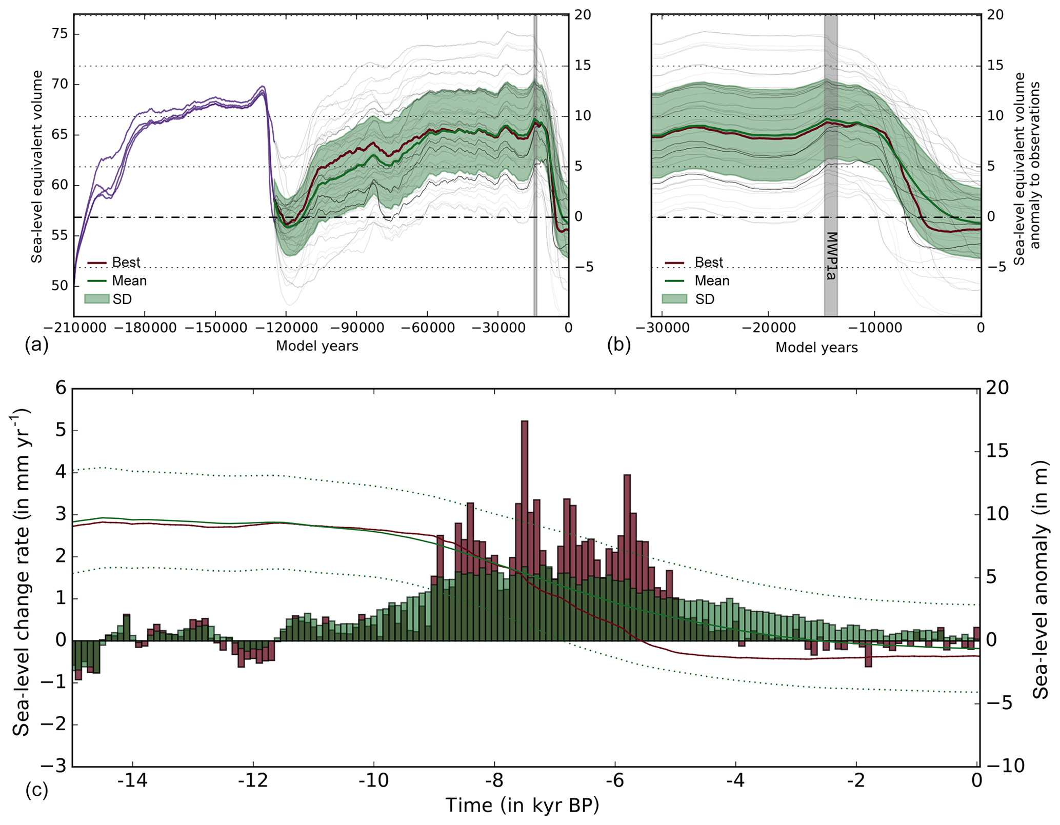
Figure 9Simulated sea-level-relevant ice volume histories over the last two glacial cycles (a) and for last deglaciation (b) for all 256 individual runs of the parameter ensemble, transparency-weighted by aggregated score. Red line indicates the best-score run, and the green line and shading indicate the score-weighted ensemble mean and standard deviation, respectively. At Last Glacial Maximum (here at 15 kyr BP) the reconstructed ensemble-mean ice volume above flotation yields 9.4±4.1 m SLE above present-day observation (compare to Figs. 5 and C4 in Pollard et al., 2016). Violet lines indicate simulations over the penultimate glacial cycle, with four different mantle viscosities which the full ensemble branches from at 125 kyr BP. During deglaciation the score-weighted ensemble mean (green) shows most of the sea-level change rates (c) between 9 and 5 kyr BP, with mean rates above 1 mm yr−1, while the best-score simulation (red) reveals rates of sea-level rise of up to 5 mm yr−1 (100 yr bins) in the same period (cf. Golledge et al., 2014, Fig. 3d). In contrast to the ensemble mean, the best-score member (red line) shows minimum ice volume in the mid-Holocene (around 4 kyr BP) and subsequent regrowth.
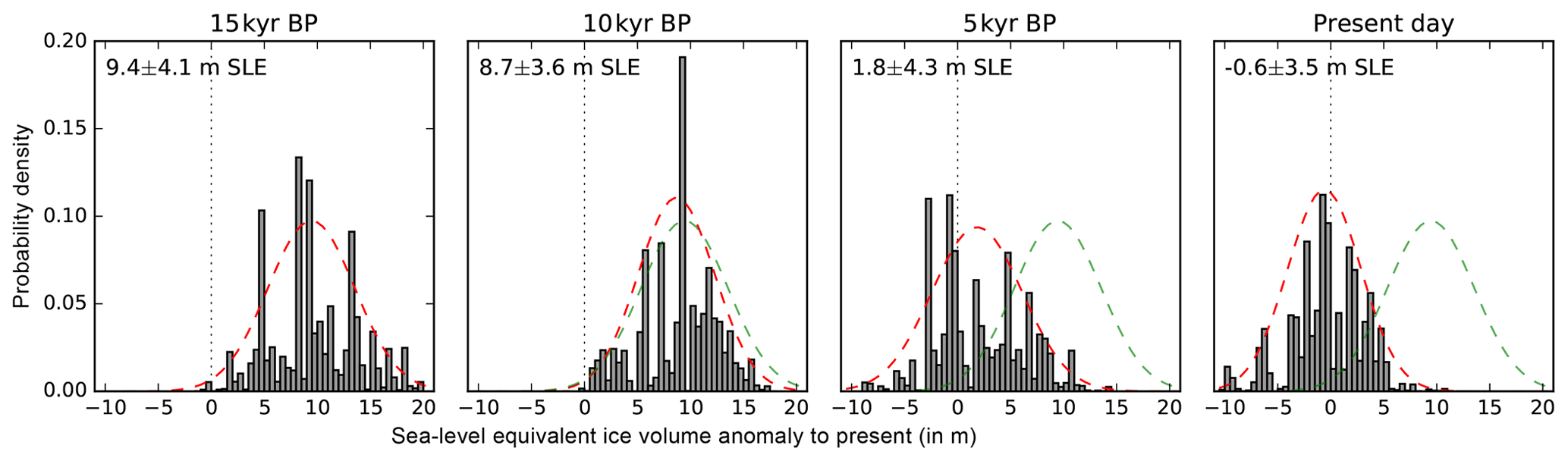
Figure 10Histogram of ensemble global mean sea-level contributions relative to modern observation at every 5 kyr over the last deglaciation period. Grey bars show the score-weighted ensemble distribution (0.5 m bins); the red curve indicates the statistically likely range (normal distribution) of the simulated ice volumes with width of 1σ standard deviation, as for the green envelope in Fig. 8. Green Gaussian curve from 15 kyr snapshot for comparison (compare to Figs. 6 and C5 in Pollard et al., 2016).
The simulations are based on the Bedmap2 dataset (Fretwell et al., 2013), remapped to 16 km resolution, which corresponds to a total grounded modern Antarctic Ice Sheet volume of 56.85 m SLE (or 26.29×10⁶ km3). The ensemble mean at the end of the simulations (in the year 2000 or −0.05 kyr BP) underestimates the observed ice volume slightly by 0.6±3.5 m SLE or, in terms of grounded ice volume, by (see Fig. 8). The histogram of score-weighted sea-level anomalies at the end of all simulations can be well approximated by a normal distribution (Fig. 9, rightmost panel). As for the LGM ice volume the ESIA parameter is also responsible for most of the present-day ice volume range of the ensemble, at more than 10 m SLE for the covered parameter range, while PREC has almost no effect, at less than 1 m SLE on average, in contrast to the LGM, as expected. VISC and PPQ reveal on average a range for the present-day ice volume of about 6 and 5 m SLE, respectively.
3.2.1 Comparison of LGM sea-level estimates in previous studies
For the maximum Antarctic ice volume at the Last Glacial Maximum, the inferred ensemble range of 5.3–13.5 m SLE excess relative to observations (or 4.5–8.5×10⁶ km3) is at the upper range found in the recent literature (Fig. 10), except for the GRISLI model results (Quiquet et al., 2018). The other previous model reconstructions are based on four different models: Glimmer (Rutt et al., 2009), PSU-ISM (or PennState3D) from Penn State University (Pollard and DeConto, 2012a), ANICE from Utrecht University (De Boer et al., 2013) and, as in this study, the Parallel Ice Sheet Model (PISM; Winkelmann et al., 2011). This section briefly compares the different model and ensemble approaches with regard to the inferred LGM ice volume estimate.
Whitehouse et al. (2012a) ran 16 Glimmer simulations at 20 km resolution with varied sliding and isostasy parameter values and different inputs for the geothermal heat flux, climatic forcing and sea-surface height. They used both geological and glaciological data to constrain the reconstruction and found the best-fit simulation at the lower end of their ensemble ice volume range. Golledge et al. (2012, 2013) used PISM on a 5 km grid for an equilibrium simulation under LGM conditions, while Golledge et al. (2014) retrieved their ensemble-mean estimates, relative to observations (Bedmap2), from an ensemble of around 250 PISM deglaciation simulations at 15 km resolution, with varied basal traction and ice-flow enhancement factors. ANICE simulations were run on 20 km resolution. In a sensitivity study, Maris et al. (2014) varied enhancement factors, till strength and (“ELRA”) bedrock deformation parameters, while in Maris et al. (2015), a small ensemble of 16 simulations with different sea-level and surface temperature forcings were applied to two different bed topographies over the last 21 kyr. Quiquet et al. (2018) varied four parameters (SIA enhancement, friction coefficient, sub-shelf melt and subglacial hydrology) in 600 equilibrium ensemble simulations with GRISLI for 40 km resolution. They selected the 12 best-thickness-fit parameters to run transient simulations over the last four glacial cycles. The relatively high estimate for the LGM ice volume is likely due to the simplified basal drag computation that does not take into account bedrock physical properties (e.g. sediments). The estimates by Briggs et al. (2014) are based on (the best 178 of) a very large ensemble of more than 3000 PSU-ISM simulations over the last two glacial cycles, at 40 km resolution, coupled with a full viscoelastic isostatic-adjustment bedrock response with a radially layered Earth viscosity profile and different treatments of sub-shelf melt, basal drag, climate forcing and calving (in total 31 varied parameters). The full ensemble range is certainly much larger, but additional constraints allow for a selection of the most realistic simulations, with most confidence in the lower part of the given range (purple error bar in Fig. 10). Pollard et al. (2016, 2017) used the PSU-ISM on 20 km resolution for an ensemble of each of the 625 simulations over the last 20 kyr and varied four parameters related to sub-shelf melt, calving, basal sliding and viscous Earth deformation, while other parameters were supposedly constrained by earlier studies. Pollard et al. (2016) applied an ELRA Earth model applied to the West Antarctic Ice Sheet only, while (Pollard et al., 2017) simulated the whole Antarctic Ice Sheet coupled to a global Earth–sea-level model. In both ensembles, ice volume change since LGM has been somewhat biased to comparably low values, as the used scoring algorithm pushed the ensemble toward a rather slippery basal sliding coefficient on modern ocean beds. As in Whitehouse et al. (2012a), Golledge et al. (2014) and this study provided anomalies based on the volume-above-flotation (VAF) calculation; the corresponding values are smaller than the directly converted values, which still include the marine part below flotation (Fig. 10b). For a conversion factor of c=2.5 our study would yield 11.3–21.3 m SLE instead. For the LGM ice volume excess relative to the modeled present-day volume, our study yields 5.9–14.1 m SLE (or 3.8–7.8×10⁶ km3), both indicated in Fig. 10.
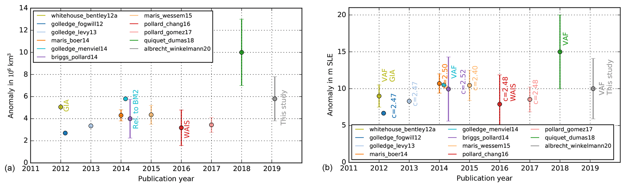
Figure 11Ice volume anomaly between Last Glacial Maximum as compared to present (not observations) in recent modeling studies in units of 106 km3 (a) and in units of meters sea-level equivalent (b). Note that the study by Pollard et al. (2016) only considers the West Antarctic subdomain in their analysis (reddish). Golledge et al. (2012, 2013, 2014) and this study used PISM (blue and grey), Maris et al. (2014, 2015) used ANICE (orange), Whitehouse et al. (2012a) used Glimmer simulations (olive), Quiquet et al. (2018) used GRISLI simulations (green), and Pollard et al. (2016, 2017) used PennState3D (or PSU-ISM) as model (blueish) coupled to different Earth models. Be aware that ice volume estimates are based on different ice densities in the different models and that different conversion factors c were used. This study, Golledge et al. (2014), as well as the Glimmer and GRISLI model, provided the volume above flotation (VAF), which subtracts some portion of the ice volume in panel (b). The provided uncertainty ranges are not necessarily symmetric; e.g. the upper range in Briggs et al. (2014) has less confidence than the lower range.
3.3 Best-fit ensemble simulation
The best-fit ensemble member simulation (no. 165; see Table 1) provides an Antarctic Ice Sheet configuration for the present day that is comparably close to observations. However, the present-day ice volume of the West Antarctic Ice Sheet is overestimated (by around 25 %), while the much larger East Antarctic Ice Sheet (EAIS) volume is rather underestimated (by around 5 %), which is also valid for the ensemble mean (Fig. ). Part of the overestimation can be explained by the relatively coarsely resolved topography of the Antarctic Peninsula and weakly constrained basal friction on the Siple Coast and Transantarctic Mountain area. This results in a root-mean-square error (RMSE) of ice thickness of 266 m (see Fig. 11a), a RMSE of grounding-line distance of 67 km (see Fig. 12) and a RMSE for surface velocities of 66 m yr−1 (see Fig. 13). The best-fit simulation also reproduces the general pattern of observed modern isostatic-adjustment rates (see Fig. 11b), with the highest uplift rates of more than 10 mm yr−1 in the Weddell and Amundsen Sea region, in agreement with GIA model reconstructions (cf. Argus et al., 2014, Fig. 6). In contrast to these GIA reconstructions, our best-fit simulation shows depression rather than uplift in the Siple Coast regions, as grounded ice is still re-advancing and hence adding load.
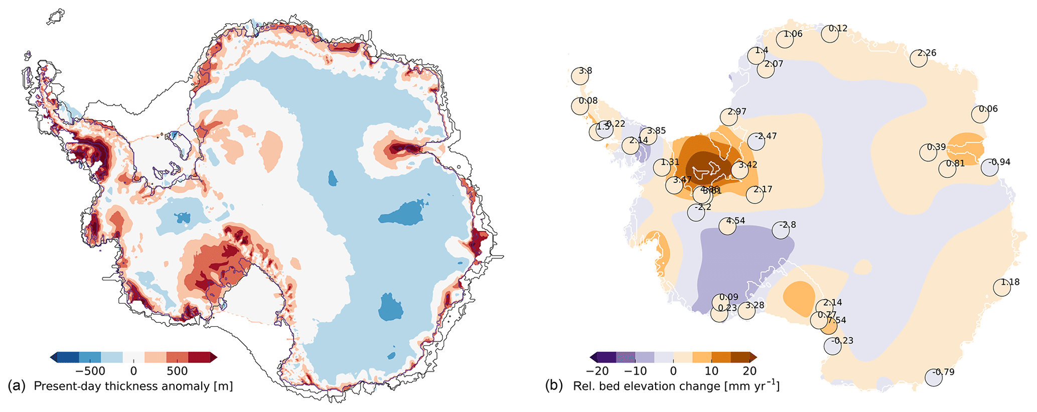
Figure 12(a) Present-day ice thickness anomaly of best-fit ensemble simulation with respect to observations (Fretwell et al., 2013), with the continental shelf in grey shades. Blue line indicates observed grounding line, while black lines indicate modeled grounding line and calving front. Large areas of the East Antarctic Ice Sheet are underestimated in ice thickness, while some marginal areas along the Antarctic Peninsula, Siple Coast and Amery Ice Shelf are thicker than observed, with a total RMSE of 266 m. (b) Modeled uplift (violet) and depression (brown) at present-day state as compared to uplift rates from recent GPS measurements (Whitehouse et al., 2012b) in 35 locations (in units mm yr−1).
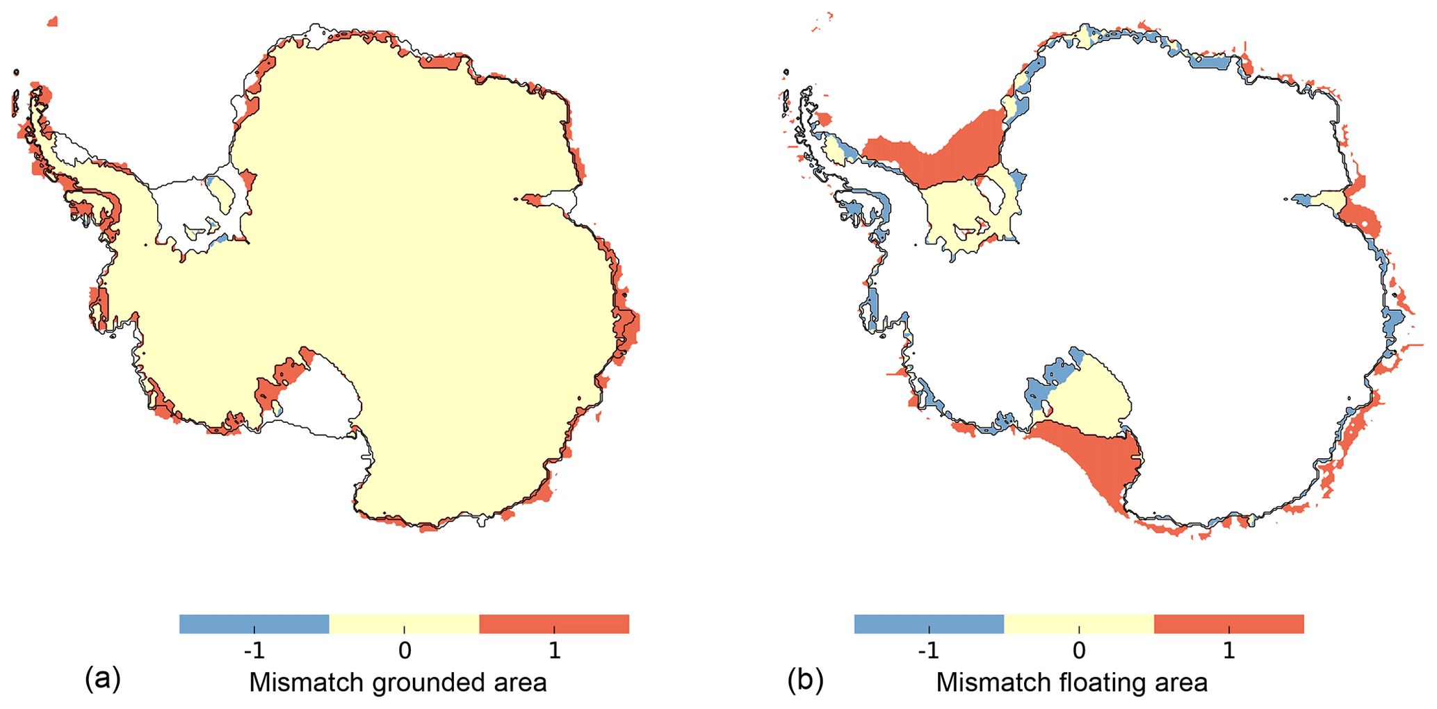
Figure 13Comparison of present-day grounded (a) and floating (b) ice extent in best-fit ensemble simulation with respect to observations (Fretwell et al., 2013). Yellow indicates a match of simulation and observations, orange means grounded and floating in model but not in observations, and blue indicates the opposite. Root-mean-square distance of modeled and observed grounding line is 67 km.
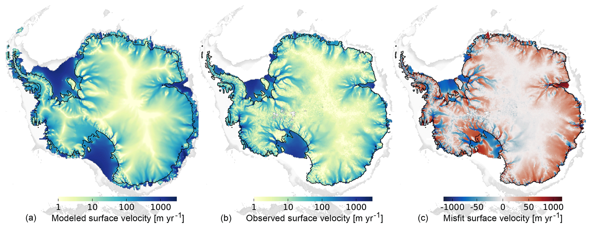
Figure 14Comparison of present-day surface velocity in best-fit ensemble simulation (a) with respect to observations (middle; Rignot et al., 2011), all on log scale. Greenish shading indicates slow-flowing regions and ice divides; blueish shading indicates regions of fast ice flow within ice shelves and far-inland-reaching ice streams. Model–observation difference is shown for observed glacierized area in (c), RMSE for surface velocities is 35 m yr−1 and mean misfit with respect to observational uncertainty is 66 m yr−1.
At the Last Glacial Maximum, at around 15 kyr BP, the sea-level-relevant volume history of the best-score simulation is close to the ensemble mean (Fig. 8), which agrees well with reconstructions by the RAISED consortium (Bentley et al., 2014, cf. Fig. 6a). The LGM state is characterized by extended ice sheet flow towards the outer Antarctic continental shelf edges, with more than 2000 m thicker ice than today in the basins of the largest modern ice shelves (Ross, Weddell, Amery and Amundsen), while the inner East Antarctic ice was a few hundred meters thinner than today (see Fig. 14).
Even though this is not the primary focus of this parameter ensemble study, it is worthwhile to have a closer look into the deglacial period. The last glacial termination (also known as Termination I, which is the end of Marine Isotope Stage 2), and hence the period of major ice sheet retreat, initiates in our best-score simulation in the Ross and Amundsen sector at around 9 kyr BP, in the Amery sector at around 8 kyr BP, and in the Weddell Sea sector at around 7 kyr BP. Maximum ice volume change rates are found accordingly in the period between 10 and 8 kyr BP, at on average SLE (or ), and in the period between 8 and 6 kyr BP, at on average SLE (or ; Fig. 15). In the 100-year running mean of the ice volume change rate we find a peak of around SLE at 7.5 kyr BP (or ; compare black and khaki line in Fig. 16). This rate of change is significantly larger than in the ensemble mean, at up to SLE, as the mean retreat becomes smoothed over a longer deglacial period (see Fig. 8c). The total ice volume change during the period 10–5 kyr BP in the best-fit simulation amounts to −9.7 m SLE. Most of this change can be attributed to increased discharge by around 1000 Gt yr−1 and increased sub-shelf melting by around 450 Gt yr−1 (partly due to increased floating ice shelf area), while surface mass balance increased only by around 300 Gt yr−1 (Fig. 16). Recent proxy-data reconstructions from the eastern Ross continental shelf suggest initial retreat not before 11.5 kyr BP (Bart et al., 2018), likely around 9–8 kyr BP (Spector et al., 2017), which is consistent with our model simulations. In the reconstructions by the RAISED consortium, most of the retreat in the Ross Sea sector (almost up to present-day grounding-line location) occurred between 10 and 5 kyr BP, while major retreat in the Weddell Sea sector likely happened before 10 kyr BP in scenario A and after 5 kyr BP in scenario B (Bentley et al., 2014, cf. Fig. 6b, c).
A Holocene minimum ice volume is reached in our simulations around 3 kyr BP with slight re-advance and thickening on the Siple Coast and Bungenstock ice rise until present day (see Fig. 15). This regrowth signal cannot be inferred from RAISED reconstructions with snapshots only every 5 kyr (Bentley et al., 2014). The corresponding mass change is rather small, at 60 Gt yr−1 (or 0.07 mm yr−1 SLE in the last 3000 years; see Fig. 16). During the late Holocene period, surface mass balance of around 3700 Gt yr−1 is balanced by approximately 2600 Gt yr−1 discharge, while sub-shelf melt plays a minor role, at around 1000 Gt yr−1.
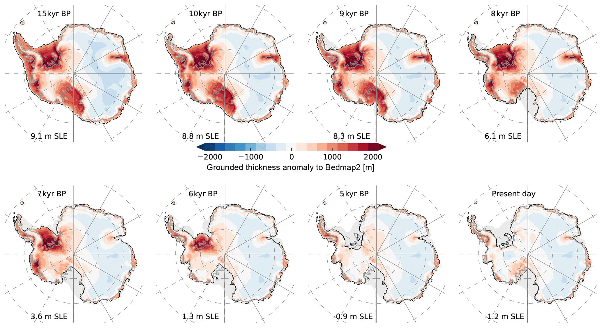
Figure 15Snapshots of grounded ice thickness anomaly to present-day observations (Fretwell et al., 2013) over last 15 kyr in best-fit simulation, analogous to Fig. 2 in Golledge et al. (2014). At LGM period grounded ice extends towards the edge of the continental shelf, with much thicker ice than present, mainly in West Antarctica. Retreat of the ice sheet occurs first in the Ross basin between 9 and 8 kyr BP, followed by the Amery basin around 1 kyr later and the Amundsen and Weddell Sea basin between 7 and 5 kyr BP. East Antarctic Ice Sheet thickness is underestimated throughout the deglaciation period (light-blue shaded area).
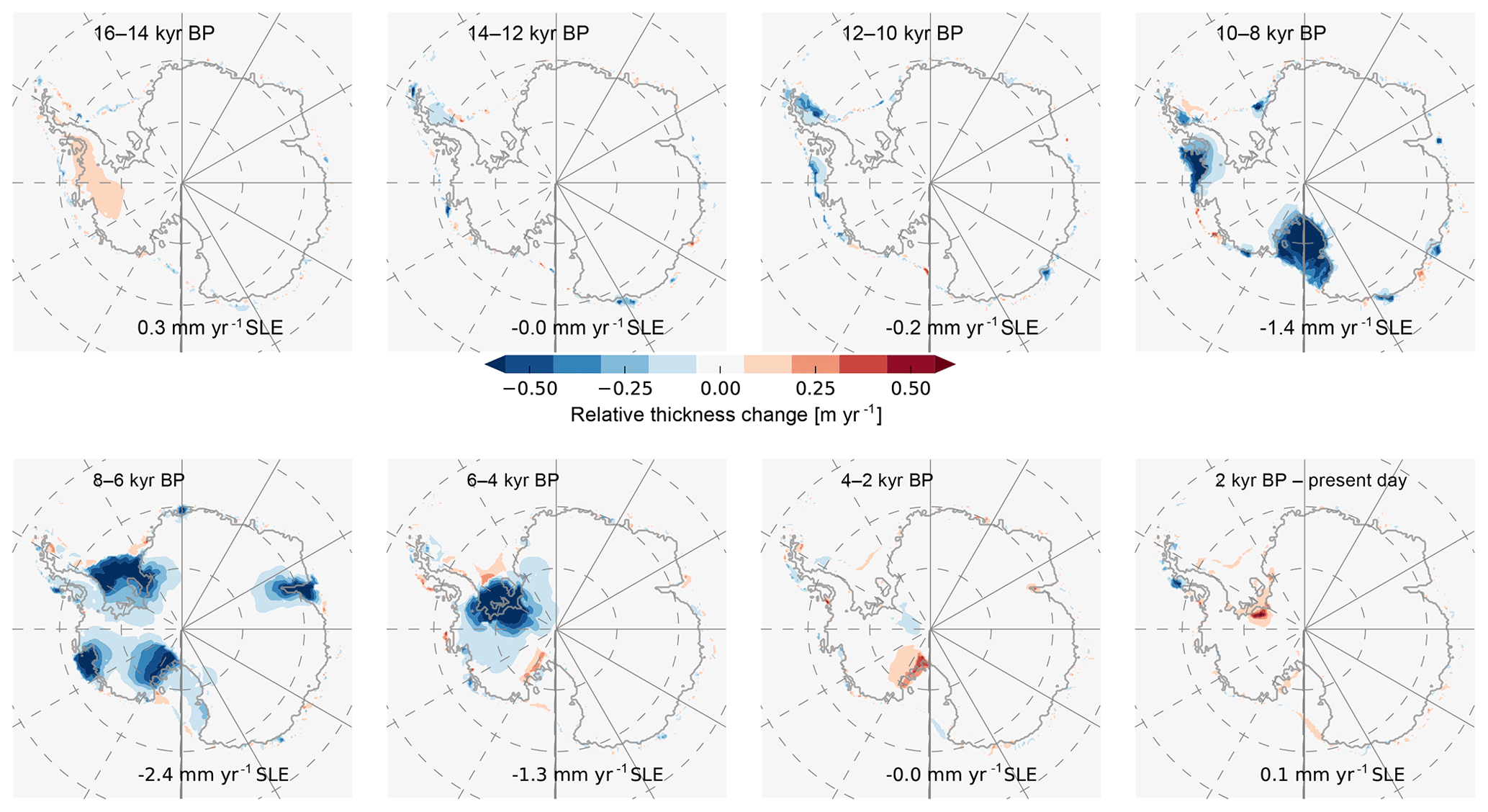
Figure 16Snapshots of relative ice thickness change rates every 2 kyr over last 16 kyr in best-fit simulation, analogous to Fig. 4 in Golledge et al. (2014). Deglaciation starts in the Ross and Amundsen sector after 10 kyr BP, with a mean change rate of SLE, followed by the Amery and Weddell Sea sector after 8 kyr BP, with mean change rates of up to SLE. In the late Holocene period since 4 kyr BP, the best-fit simulation shows some thickening on the Siple Coast and in the Bungenstock Ice Rise, corresponding to about SLE.
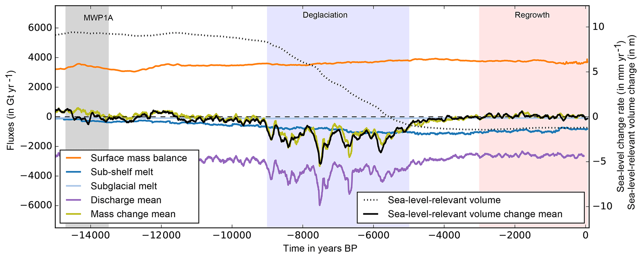
Figure 17Mass fluxes over the last 15 kyr for the best-fit simulation (y axis), with the sum of surface (orange) and basal mass balance (blue; subglacial melt in light blue is negligible) and discharge (100-year running mean in violet) yielding total mass change (khaki). Mass change agrees well with sea-level-relevant volume change (100-year running mean in black; x axis). Main deglaciation occurs between 9 and 5 kyr BP (black dotted line; x axis), at on average 2.0 mm yr−1, or 1000 Gt yr−1 (blue bar), significantly after MWP1a (grey bar). In the last 3 kyr of the best-fit simulation, the Antarctic Ice Sheet regains mass by about 60 Gt yr−1, which equals about 0.07 mm yr−1 SLE (red bar).
3.4 Discussion of individual ensemble parameters
In this section we discuss the effects of individual ensemble parameters in more detail and also in comparison to previous model studies. We performed our analysis for an ensemble of 256 simulations of the entire Antarctic Ice Sheet over the last two glacial cycles, with 16 km grid resolution, using PISM. The parameter ensemble is spanned by four model parameters (Sect. 2.1); two of them are more relevant to glacial dynamics in the West Antarctic Ice Sheet (VISC and PPQ), while the other two are more related to glacial ice volume change in the East Antarctic Ice Sheet (ESIA and PREC; see overview in Sect. 2.1).
For the bedrock response, we chose the upper-mantle viscosity as one ensemble parameter and found maximum scores around values of for all of Antarctica. This corresponds to a rebound timescale of 1000–3000 years, which is in line with the findings in Maris et al. (2014) and Pollard et al. (2016) for WAIS, using a simplified Earth model (ELRA). Pollard et al. (2017), in contrast, used the same ensemble analysis tools for the whole continent of Antarctica and varied the vertical viscoelastic profiles of the Earth within a gravitationally self-consistent coupled Earth–sea-level model. They found only little difference in simulated glacial volumes to modern ice volumes for different viscosity profiles bounded between 1 × 10¹⁹ and 5 × 10²¹ Pa s. Briggs et al. (2014) have not varied viscoelastic Earth model components, assuming that the impact of climatic forcing, for instance, is more relevant.
For the basal sliding, we decided on the sliding exponent PPQ as an uncertain ensemble parameter. A value of 0.0 corresponds to Coulomb friction, as used in the PSU-ISM simulations, while ANICE used a value of 0.3 (Maris et al., 2014) and Quiquet et al. (2018) a linear scaling (1.0). Interestingly, we find best scores for rather high sliding exponents of PPQ, with values of 0.75 or 1.0 (rather linear relationship of sliding velocity and till strength).
Briggs et al. (2013) used Coulomb friction and varied instead three parameters that control the basal sliding over soft and hard beds, based on an erosion parameterization. In our study, the till weakness is associated with the till friction angle, which is optimized for the present-day grounded Antarctic Ice Sheet (Pollard and DeConto, 2012b). In Briggs et al. (2013), basal sliding additionally accounts for basal roughness and pinning points (three parameters), which are otherwise underestimated as a result of the coarse model resolution.
Another sliding-related key parameter is the friction coefficient underneath the modern ice shelves, as varied in Pollard et al. (2016, 2017), who found it to be the most dominant ensemble parameter. As discussed in the companion paper (Albrecht et al., 2020), we also find till properties in the ice shelf regions to be highly relevant, in particular during deglaciation. As a consequence, we ran an additional ensemble analysis for four parameters associated with basal sliding and hydrology, including friction underneath modern ice shelves, and discussed the results in the Supplement (Sect. A). In the best-fit simulations of this “basal ensemble”, we find main deglacial retreat occurring a few thousand years earlier (closer to MWP1a) than in the base ensemble. Hence, the corresponding scores are even better than for the best-fit simulation of the base ensemble, for same sliding exponent but a smaller minimal till friction angle of ≤1∘.
For a representation of the ice dynamical uncertainty we chose the ESIA enhancement factor as the most relevant ensemble parameter, which mainly affects the grounded ice volume. We find best fits for rather small ESIA values of 1.0–2.0, while for larger values the modeled EAIS ice thickness underestimates modern observations. Pollard et al. (2016) did not vary enhancement factors in their ensemble and used a rather small enhancement factor of 1.0 for the SIA, while the value for the SSA enhancement was prescribed to a very low value of 0.3 (Pollard and DeConto, 2012a). Briggs et al. (2014) varied enhancement factors for both the SIA and SSA in their large ensemble and determined a rather large reference value of 4.8 for SIA enhancement and a reference value close to 0.6 for SSA enhancement (see Table 1 in Briggs et al., 2013), which we used in all our ensemble simulations. Maris et al. (2014) determined, in their sensitivity study for the SIA enhancement, an even larger reference value of 9.0, and for the SSA enhancement, they determined a value of 0.8. In Quiquet et al. (2018) best fits to present-day thickness are found to be between 1.5 and 4.0 and between 0.2 and 0.5 for SIA and SSA enhancement, respectively.
As the climate-related uncertain ensemble parameter, we chose a parameter associated with the change of precipitation with temperatures, PREC. The best-fit parameter values of PREC=7 % K−1–10 % K−1 yield, for 10 K colder glacial temperatures, about 50 %–65 % less precipitation. This parameter is similar to the insolation scaling parameter in Briggs et al. (2013), where the best-fit value would result in about 60 % less precipitation at the insolation minimum. In total, Briggs et al. (2014) varied seven precipitation-related parameters based on three different precipitation forcings (one of which is similar to the one we used). Maris et al. (2014) used instead a linear temperature-based scaling between the LGM and present-day surface mass balance (with about 58 % anomaly) with a fixed parameter.
Beyond the four parameters varied in our ensemble, previous ensemble studies found, for instance, high sensitivity in at least one of the five temperature-related parameters (Briggs et al., 2013). In contrast, we found only little effect of temperature-related parameter variation on the sea-level-relevant ice sheet volume, as discussed in the companion paper (Albrecht et al., 2020). Concerning iceberg calving, Pollard et al. (2016) included one related parameter in their ensemble analysis, while Briggs et al. (2013) varied three parameters for ice shelf calving and one parameter for tidewater calving. Our “eigencalving” parameterization also uses a strain-rate-based calving estimate, combined with a minimal terminal ice thickness, and provides a representation of calving front dynamics, which, to the first order, yields calving front locations close to present observations (Levermann et al., 2012). As this parameterization is rather independent of the climate conditions, variations in the eigencalving parameter show only little effect on sea-level-relevant ice volume (see Albrecht et al., 2020; Sect. 2.4).
Regarding sub-shelf melting, Pollard et al. (2016) and Quiquet et al. (2018) included one uncertain parameter in their analysis, while Briggs et al. (2013) even varied four melt-related parameters. We used the PICO model that includes physics to adequately represent melting and refreezing (Reese et al., 2018). The two key PICO parameters were constrained for present observations so that we preferred other less constrained parameters in our ensemble that are more relevant to the ice volume history of the Antarctic Ice Sheet. Also, for variation in the scaling constant of ocean input temperatures with surface temperature, the glacial ice volume showed a comparably low sensitivity (see Sect. 4.3 in companion paper; Albrecht et al., 2020).
The four selected ensemble parameters, representing uncertainties in interacting ice–Earth dynamics, basal sliding and climate conditions, imply a large range of uncertainty for the total Antarctic ice volume change. They were chosen such that the model yields a present-day ice volume close to observations, while the LGM ice volume differs significantly for parameter change. The probed parameter range has been chosen to be rather broad, which implies a low sampling density of the parameter space. With the knowledge gained in this ensemble analysis, this range could be further constrained in a (larger) sub-ensemble. Also, other parameters may be more relevant to certain regions of the Antarctic Ice Sheet or for the onset and rate of the last deglaciation, which in our ensemble occurs generally later than suggested by many paleo-records. A closer look into the details of the deglacial period and relevant parameters will be discussed in a separate follow-up study.
One deficiency of our model settings is the general underestimation of ice thickness in the inner ice sheet sections of up to −500 m, mainly in the EAIS, which could be a result of the underestimated RACMO precipitation. In contrast, ice thickness is overestimated in the outer terminal regions and at the Siple Coast by up to 500 m, where the complex topography is not sufficiently resolved in the model, with implications for inferred basal conditions and temperature conditions. Accordingly, we find a considerable misfit to most paleo-elevation data (ELEV), which are located mainly in the marginal mountain regions. This could be improved, e.g. by parameterized basal roughness or erosion, as proposed in Briggs et al. (2013), or by higher model resolution and updated bed topography datasets (e.g. Morlighem et al., 2019).
The score aggregation scheme according to Pollard et al. (2016) implies that the paleo-data types have equal influence to the present-day constraints, although they cover only a relatively small regions and periods of the modeled ice sheet history (Briggs and Tarasov, 2013). However, as the variability in paleo-misfits is comparably low among the ensemble, these data types have only relatively small imprint on the aggregated score (see more details in Sect. B). This is also valid for a data-type weighted score (Briggs and Tarasov, 2013), which, applied to our ensemble results, yields a similar set of best-score runs.
Further work will consist of the determination of more realistic climate reconstructions using general circulation model results and in the explicit computation of the local relative sea level, which could potentially have an strong impact on grounding-line migration for glacial cycles (Gomez et al., 2013).
We ran an ensemble of 256 simulations over the last two glacial cycles and applied a simple averaging method with full-factorial sampling similar to Pollard et al. (2016). Although this kind of ensemble method is limited to a comparably small number of values for each parameter, and hence the retrieved scores are somewhat blocky (as compared to advanced techniques that can interpolate in parameter space), we still recognize a general pattern of parameter combinations that provide best model fits to both present-day observations and paleo-records. However, the selected ensemble parameters certainly cannot cover the full range of possible model response, in particular with regard to the self-amplifying effects during deglaciation.
For the four sampled parameters, best fits are found for mantle viscosity around VISC=0.5–2.5×10²¹ Pa s, for rather linear relationships between sliding speed and till strength (with exponents PPQ=0.75–1.0), for no or only small enhancement of the SIA-derived flow speed (with ESIA=1.0–2.0), and for rather high rates of relative precipitation change with temperature forcing (). The five best-score ensemble members fall within this range. In comparison to the best-fit member (, , PPQ=0.75 and ESIA=2.0), slightly more sliding (PPQ=1.0) or slower ice flow (ESIA=1.0) can compensate for relatively dry climate conditions in colder climates for higher PREC values, which is associated with smaller ice volumes and hence smaller driving stresses. The strongest effects of varying ESIA and PREC parameters are found for the much larger East Antarctic Ice Sheet volume, while PPQ and VISC have the most pronounced effects for the West Antarctic Ice Sheet dynamics in terms of grounding-line migration and induced changes in ice loading.
The grounding line extends at Last Glacial Maximum to the edge of the continental shelf for nearly all simulations. The onset and rate of deglaciation, however, are very sensitive to the choice of parameters and boundary conditions, in particular those related to basal sliding. Due to the comparably coarse resolution and the high uncertainty (sensitivity) that comes with the strong nonlinearity of the system, we discuss here general patterns of reconstructed ice sheet histories rather than exact numbers, which would require a much larger ensemble with an extended number of varied parameters.
The score-weighted likely range (1 standard deviation) of our reconstructed ice volume histories suggests a contribution of the Antarctic Ice Sheet to the global mean sea level since the Last Glacial Maximum at around 15 kyr BP of 9.4±4.1 m SLE (). The ensemble-mean ice volume anomaly between LGM and present is therefore slightly higher than in most recently published studies. The choice of basal sliding parameterization in the different models seems to have most impact on the corresponding estimates. The ensemble reproduces the observed present-day grounded ice volume with an score-weighted anomaly of 0.6±3.5 m SLE () and hence serves as a suitable initial state for future projections.
The reconstructed score-weighted ensemble range (1σ) is comparably large, at up to 4.3 m SLE (or 2.0×10⁶ km3), which can be explained by a high model sensitivity (Albrecht et al., 2020), by a comparably large range of the sampled parameter values and of course by the choice of the aggregated score scheme. By using “sieve” criteria the ensemble range could be reduced. For the much larger ensemble study when covering 31 parameters (Briggs et al., 2014) a narrowed ensemble range of 4.4 m ESL (different definition of sea-level equivalent volume change) or 1.8×10⁶ km3 was found for the best 5 % of the ensemble simulations, which is close to the range of our study.
The onset of deglaciation and hence major grounding-line retreat occurs in our model simulations after 12 kyr BP and hence well after MWP1a (≈14.3 kyr BP). A previous PISM study simulated much earlier and larger sea-level contributions from Antarctica for oceanic forcing at intermediate levels that are anticorrelated to the surface temperature forcing (Golledge et al., 2014), as likely happened during the 2 millennia of Antarctic Cold Reversal following the MWP1a.
The PISM model results in Kingslake et al. (2018) are based on this ensemble study but have been published before with a slightly older model version (see data and model code availability therein). Meanwhile, we have improved the Earth model, which accounts for changes in the ocean water column induced by variations in bed topography or sea-level changes. In contrast to Kingslake et al. (2018), we used the remapped topography without local adjustment in the region of Bungenstock ice rise in the Weddell Sea sector and found, in about 20 % of the score-weighted simulations, an extensive retreat of the grounding line and subsequent re-advance in both the Ross and Weddell Sea sector.
The paleo-simulation ensemble analysis presented here provides a set of data-constrained parameter combinations for PISM simulations that can be used as a reference for further sensitivity studies investigating specific episodes in the history of Antarctica, such as the last deglaciation or the Last Interglacial, as well as for projections of Antarctic sea-level contributions.
The PISM code used in this study can be obtained from https://doi.org/10.5281/zenodo.3574032 (Albrecht and PISM authors, 2019); most model improvements have been merged into the latest PISM development at https://github.com/pism/pism (last access: 9 February 2020; The PISM authors, 2020a). PISM input data are preprocessed using https://github.com/pism/pism-ais (last access: 9 February 2020; The PISM authors, 2020c). Results and plotting scripts are available from https://doi.org/10.1594/PANGAEA.909728 (Albrecht, 2019b). The scoring scheme with respect to modern and paleo-data can be downloaded from https://doi.org/10.5281/zenodo.3585118 (Albrecht, 2019c).
The supplement related to this article is available online at: https://doi.org/10.5194/tc-14-633-2020-supplement.
TA designed, ran and analyzed the ice sheet model experiments. TA and RW co-developed PISM and implemented processes relevant to application to the Antarctic Ice Sheet. RW and AL contributed to the interpretation of the results.
The authors declare that they have no conflict of interest.
Development of PISM is supported by NASA grant NNX17AG65G and NSF grants PLR-1603799 and PLR-1644277. Open-source software was used at all stages, in particular NumPy (https://numpy.org, last access: 9 February 2020), CDO (https://code.mpimet.mpg.de/projects/cdo, last access: 9 February 2020), NCO (http://nco.sourceforge.net, last access: 9 February 2020) and Matplotlib (https://matplotlib.org, last access: 9 February 2020). The authors gratefully acknowledge the European Regional Development Fund (ERDF), the German Federal Ministry of Education and Research, and the state of Brandenburg for supporting this project by providing resources on the high-performance computer system at the Potsdam Institute for Climate Impact Research. Computer resources for this project have been also provided by the Gauss Centre for Supercomputing and Leibniz Supercomputing Centre (https://www.lrz.de, last access: 9 February 2020) under project ID pr94ga and pn69ru. Torsten Albrecht is supported by the Deutsche Forschungsgemeinschaft (DFG) in the framework of the priority program “Antarctic Research with comparative investigations in Arctic ice areas”. We thank Dave Pollard for sharing ensemble analysis scripts and for valuable discussions and Stewart Jamieson for sharing gridded RAISED datasets. Finally, we appreciate the assistance by the editor Alexander Robinson and the many helpful suggestions and comments by Lev Tarasov and an anonymous reviewer, which led to considerable improvements of the paper.
This research has been supported by the Deutsche Forschungsgemeinschaft (grant nos. LE1448/6-1, LE1448/7-1 and WI14556/4-1), NASA (grant no. NNX17AG65G), the NSF (grant nos. PLR-1603799 and PLR-1644277), and the Gauss Centre for Supercomputing and Leibniz Supercomputing Centre (grant nos. pn69ru and pr94ga).
The article processing charges for this open-access publication were covered by the Potsdam Institute for Climate Impact Research (PIK).
This paper was edited by Alexander Robinson and reviewed by Lev Tarasov and one anonymous referee.
Albrecht, T.: PISM parameter ensemble analysis of Antarctic Ice Sheet glacial cycle simulations, PANGAEA, https://doi.org/10.1594/PANGAEA.909728, 2019b. a
Albrecht, T.: PISM ensemble scoring: Parameter ensemble analysis tools as used in Albrecht et al., 2020, The Cryosphere, Zenodo, https://doi.org/10.5281/zenodo.3585118, 2019c. a
Albrecht, T. and PISM authors: PISM version as used in Albrecht et al., 2020, The Cryosphere, Zenodo, https://doi.org/10.5281/zenodo.3574032, 2019. a
Albrecht, T., Winkelmann, R., and Levermann, A.: Glacial-cycle simulations of the Antarctic Ice Sheet with the Parallel Ice Sheet Model (PISM) – Part 1: Boundary conditions and climatic forcing, The Cryosphere, 14, 599–632, https://doi.org/10.5194/tc-14-599-2020, 2020. a, b, c, d, e, f, g, h, i, j, k, l
Argus, D. F., Peltier, W., Drummond, R., and Moore, A. W.: The Antarctica component of postglacial rebound model ICE-6G_C (VM5a) based on GPS positioning, exposure age dating of ice thicknesses, and relative sea level histories, Geophys. J. Int., 198, 537–563, 2014. a
Aschwanden, A. and Blatter, H.: Mathematical modeling and numerical simulation of polythermal glaciers, J. Geophys. Res.-Earth Surf., 114, F01027, https://doi.org/10.1029/2008JF001028, 2009. a
Aschwanden, A., Bueler, E., Khroulev, C., and Blatter, H.: An enthalpy formulation for glaciers and ice sheets, J. Glaciol., 58, 441–457, https://doi.org/10.3189/2012JoG11J088, 2012. a, b
Barletta, V. R., Bevis, M., Smith, B. E., Wilson, T., Brown, A., Bordoni, A., Willis, M., Khan, S. A., Rovira-Navarro, M., Dalziel, I., Smalley, R., Kendrick, E., Konfal, S., Caccamise, D. J., Aster, R. C., Nyblade, A., and Wiens, D. A.: Observed rapid bedrock uplift in Amundsen Sea Embayment promotes ice-sheet stability, Science, 360, 1335–1339, 2018. a
Bart, P. J., Mullally, D., and Golledge, N. R.: The influence of continental shelf bathymetry on Antarctic Ice Sheet response to climate forcing, Global Planet. Change, 142, 87–95, 2016. a
Bart, P. J., DeCesare, M., Rosenheim, B. E., Majewski, W., and McGlannan, A.: A centuries-long delay between a paleo-ice-shelf collapse and grounding-line retreat in the Whales Deep Basin, eastern Ross Sea, Antarctica, Sci. Rep., 8, 1–9, https://doi.org/10.1038/s41598-018-29911-8, 2018. a
Bentley, M. J., Ó Cofaigh, C., Anderson, J. B., Conway, H., Davies, B., Graham, A. G. C., Hillenbrand, C.-D., Hodgson, D. A., Jamieson, S. S. R., Larter, R. D., Mackintosh, A., Smith, J. A., Verleyen, E., Ackert, R. P., Bart, P. J., Berg, S., Brunstein, D., Canals, M., Colhoun, E. A., Crosta, X., Dickens, W. A., Domack, E., Dowdeswell, J. A., Dunbar, R., Ehrmann, W., Evans, J., Favier, V., Fink, D., Fogwill, C. J., Glasser, N. F., Gohl, K., Golledge, N. R., Goodwin, I., Gore, D. B., Greenwood, S. L., Hall, B. L., Hall, K., Hedding, D. W., Hein, A. S., Hocking, E. P., Jakobsson, M., Johnson, J. S., Jomelli, V., Jones, R. S., Klages, J. P., Kristoffersen, Y., Kuhn, G., Leventer, A., Licht, K., Lilly, K., Lindow, J., Livingstone, S. J., Massé, G., McGlone, M. S., McKay, R. M., Melles, M., Miura, H., Mulvaney, R., Nel, W., Nitsche, F. O., O'Brien, P. E., Post, A. L., Roberts, S. J., Saunders, K. M., Selkirk, P. M., Simms, A. R., Spiegel, C., Stolldorf, T. D., Sugden, D. E., van der Putten, N., van Ommen, T., Verfaillie, D., Vyverman, W., Wagner, B., White, D. A., Witus, A. E., and Zwartz, D.: A community-based geological reconstruction of Antarctic Ice Sheet deglaciation since the Last Glacial Maximum, Quaternary Sci. Rev., 100, 1–9, https://doi.org/10.1016/j.quascirev.2014.06.025, 2014. a, b, c, d, e, f
Briggs, R., Pollard, D., and Tarasov, L.: A glacial systems model configured for large ensemble analysis of Antarctic deglaciation, The Cryosphere, 7, 1949–1970, https://doi.org/10.5194/tc-7-1949-2013, 2013. a, b, c, d, e, f, g, h, i
Briggs, R. D. and Tarasov, L.: How to evaluate model-derived deglaciation chronologies: a case study using Antarctica, Quaternary Sci. Rev., 63, 109–127, 2013. a, b, c, d, e, f, g, h, i, j, k
Briggs, R. D., Pollard, D., and Tarasov, L.: A data-constrained large ensemble analysis of Antarctic evolution since the Eemian, Quaternary Sci. Rev., 103, 91–115, https://doi.org/10.1016/j.quascirev.2014.09.003, 2014. a, b, c, d, e, f, g, h, i, j
Bueler, E. and Brown, J.: Shallow shelf approximation as a “sliding law” in a thermomechanically coupled ice sheet model, J. Geophys. Res., 114, F03008, https://doi.org/10.1029/2008JF001179, 2009. a
Bueler, E. and van Pelt, W.: Mass-conserving subglacial hydrology in the Parallel Ice Sheet Model version 0.6, Geosci. Model Dev., 8, 1613–1635, https://doi.org/10.5194/gmd-8-1613-2015, 2015. a
Bueler, E., Lingle, C. S., and Brown, J.: Fast computation of a viscoelastic deformable Earth model for ice-sheet simulations, Ann. Glaciol., 46, 97–105, 2007. a, b
Cuffey, K. M. and Marshall, S. J.: Substantial contribution to sea-level rise during the last interglacial from the Greenland ice sheet, Nature, 404, 591, 2000. a
Cuffey, K. M. and Paterson, W. S. B.: The physics of glaciers, Academic Press, 2010. a
Cuffey, K. M., Clow, G. D., Steig, E. J., Buizert, C., Fudge, T., Koutnik, M., Waddington, E. D., Alley, R. B., and Severinghaus, J. P.: Deglacial temperature history of West Antarctica, P. Natl. Acad. Sci. USA, 113, 14249–14254, 2016. a
De Boer, B., Van de Wal, R., Lourens, L., Bintanja, R., and Reerink, T.: A continuous simulation of global ice volume over the past 1 million years with 3-D ice-sheet models, Clim. Dynam., 41, 1365–1384, 2013. a
Fogwill, C. J., Turney, C. S. M., Golledge, N. R., Etheridge, D. M., Rubino, M., Thornton, D. P., Baker, A., Woodward, J., Winter, K., Van Ommen, T. D., Moy, A. D., Curran, M. A. J., Davies, S. M., Weber, M. E., Bird, M. I., Munksgaard, N. C., Menviel, L., Rootes, C. M., Ellis, B., Millman, H., Vohra, J., Rivera, A., and Cooper, A.: Antarctic ice sheet discharge driven by atmosphere-ocean feedbacks at the Last Glacial Termination, Sci. Rep., 7, 39979, https://doi.org/10.1038/srep39979, 2017. a
Fretwell, P., Pritchard, H. D., Vaughan, D. G., Bamber, J. L., Barrand, N. E., Bell, R., Bianchi, C., Bingham, R. G., Blankenship, D. D., Casassa, G., Catania, G., Callens, D., Conway, H., Cook, A. J., Corr, H. F. J., Damaske, D., Damm, V., Ferraccioli, F., Forsberg, R., Fujita, S., Gim, Y., Gogineni, P., Griggs, J. A., Hindmarsh, R. C. A., Holmlund, P., Holt, J. W., Jacobel, R. W., Jenkins, A., Jokat, W., Jordan, T., King, E. C., Kohler, J., Krabill, W., Riger-Kusk, M., Langley, K. A., Leitchenkov, G., Leuschen, C., Luyendyk, B. P., Matsuoka, K., Mouginot, J., Nitsche, F. O., Nogi, Y., Nost, O. A., Popov, S. V., Rignot, E., Rippin, D. M., Rivera, A., Roberts, J., Ross, N., Siegert, M. J., Smith, A. M., Steinhage, D., Studinger, M., Sun, B., Tinto, B. K., Welch, B. C., Wilson, D., Young, D. A., Xiangbin, C., and Zirizzotti, A.: Bedmap2: improved ice bed, surface and thickness datasets for Antarctica, The Cryosphere, 7, 375–393, https://doi.org/10.5194/tc-7-375-2013, 2013. a, b, c, d, e, f, g, h, i, j, k, l, m
Frieler, K., Clark, P. U., He, F., Buizert, C., Reese, R., Ligtenberg, S. R. M., van den Broeke, M. R., Winkelmann, R., and Levermann, A.: Consistent evidence of increasing Antarctic accumulation with warming, Nat. Clim. Change, 5, 348–352, https://doi.org/10.1038/nclimate2574, 2015. a
Golledge, N. R., Fogwill, C. J., Mackintosh, A. N., and Buckley, K. M.: Dynamics of the last glacial maximum Antarctic ice-sheet and its response to ocean forcing, P. Natl. Acad. Sci., 109, 16052–16056, 2012. a, b
Golledge, N. R., Levy, R. H., McKay, R. M., Fogwill, C. J., White, D. A., Graham, A. G., Smith, J. A., Hillenbrand, C.-D., Licht, K. J., Denton, G. H., Ackert Jr., R. P., Maas, S. M., and Hall, B. L.: Glaciology and geological signature of the Last Glacial Maximum Antarctic ice sheet, Quaternary Sci. Rev., 78, 225–247, https://doi.org/10.1016/j.quascirev.2013.08.011, 2013. a, b
Golledge, N. R., Menviel, L., Carter, L., Fogwill, C. J., England, M. H., Cortese, G., and Levy, R. H.: Antarctic contribution to meltwater pulse 1A from reduced Southern Ocean overturning, Nat. Commun., 5, 5107, https://doi.org/10.1038/ncomms6107, 2014. a, b, c, d, e, f, g, h, i, j, k
Gomez, N., Pollard, D., and Mitrovica, J. X.: A 3-D coupled ice sheet–sea level model applied to Antarctica through the last 40 ky, Earth Planet. Sci. Lett., 384, 88–99, 2013. a
Jenkins, A., Shoosmith, D., Dutrieux, P., Jacobs, S., Kim, T. W., Lee, S. H., Ha, H. K., and Stammerjohn, S.: West Antarctic Ice Sheet retreat in the Amundsen Sea driven by decadal oceanic variability, Nat. Geosci., 11, 733–738, 2018. a
Jouzel, J., Masson-Delmotte, V., Cattani, O., Dreyfus, G., Falourd, S., Hoffmann, G., Minster, B., Nouet, J., Barnola, J. M., Chappellaz, J., Fischer, H., Gallet, J. C., Johnsen, S., Leuenberger, M., Loulergue, L., Luethi, D., Oerter, H., Parrenin, F., Raisbeck, G., Raynaud, D., Schilt, A., Schwander, J., Selmo, E., Souchez, R., Spahni, R., Stauffer, B., Steffensen, J. P., Stenni, B., Stocker, T. F., Tison, J. L., Werner, M., and Wolff, E. W.: Orbital and Millennial Antarctic Climate Variability over the Past 800,000 Years, Science, 317, 793–796, https://doi.org/10.1126/science.1141038, 2007. a
Kingslake, J., Scherer, R., Albrecht, T., Coenen, J., Powell, R., Reese, R., Stansell, N., Tulaczyk, S., Wearing, M., and Whitehouse, P.: Extensive retreat and re-advance of the West Antarctic ice sheet during the Holocene, Nature, 558, 430–434, https://doi.org/10.1038/s41586-018-0208-x, 2018. a, b, c, d, e, f, g
Kopp, R. E., Simons, F. J., Mitrovica, J. X., Maloof, A. C., and Oppenheimer, M.: Probabilistic assessment of sea level during the last interglacial stage, Nature, 462, 863–867, 2009. a
Levermann, A., Albrecht, T., Winkelmann, R., Martin, M. A., Haseloff, M., and Joughin, I.: Kinematic first-order calving law implies potential for abrupt ice-shelf retreat, The Cryosphere, 6, 273–286, https://doi.org/10.5194/tc-6-273-2012, 2012. a
Lingle, C. S. and Clark, J. A.: A numerical model of interactions between a marine ice sheet and the solid earth: Application to a West Antarctic ice stream, J. Geophys. Res.-Oceans, 90, 1100–1114, 1985. a
Liu, J., Milne, G. A., Kopp, R. E., Clark, P. U., and Shennan, I.: Sea-level constraints on the amplitude and source distribution of Meltwater Pulse 1A, Nat. Geosci., 9, 130–134, https://doi.org/10.1038/ngeo2616, 2016. a
Maris, M. N. A., de Boer, B., Ligtenberg, S. R. M., Crucifix, M., van de Berg, W. J., and Oerlemans, J.: Modelling the evolution of the Antarctic ice sheet since the last interglacial, The Cryosphere, 8, 1347–1360, https://doi.org/10.5194/tc-8-1347-2014, 2014. a, b, c, d, e, f, g
Maris, M., Van Wessem, J., Van De Berg, W., De Boer, B., and Oerlemans, J.: A model study of the effect of climate and sea-level change on the evolution of the Antarctic Ice Sheet from the Last Glacial Maximum to 2100, Clim. Dynam., 45, 837–851, 2015. a, b, c, d, e, f
Martos, Y. M., Catalán, M., Jordan, T. A., Golynsky, A., Golynsky, D., Eagles, G., and Vaughan, D. G.: Heat flux distribution of Antarctica unveiled, Geophys. Res. Lett., 44, 11417–11426, https://doi.org/10.1002/2017GL075609, 2017. a
Mercer, J. H.: West Antarctic ice sheet and CO2 greenhouse effect: a threat of disaster, Nature, 271, 321–325, 1978. a, b
Morland, L. and Johnson, I.: Steady motion of ice sheets, J. Glaciol., 25, 229–246, 1980. a
Morlighem, M., Rignot, E., Binder, T., Blankenship, D. D., Drews, R., Eagles, G., Eisen, O., Ferraccioli, F., Forsberg, R., Fretwell, P., Goel, V., Greenbaum, J. S., Gudmundsson, H., Guo, J., Helm, V., Hofstede, C., Howat, I., Humbert, A., Jokat, W., Karlsson, N. B., Lee, W., Matsuoka, K., Millan, R., Mouginot, J., Paden, J., Pattyn, F., Roberts, J. L., Rosier, S., Ruppel, A., Seroussi, H., mith, E. C., Steinhage, D., Sun, B., van den Broeke, M. R., van Ommen, T., van Wessem, M., and Young, D. A.: Deep glacial troughs and stabilizing ridges unveiled beneath the margins of the Antarctic ice sheet, Nat. Geosci., 13, 132–137, https://doi.org/10.1038/s41561-019-0510-8, 2019. a
Oppenheimer, M. and Alley, R. B.: How high will the seas rise?, Science, 354, 1375–1377, 2016. a
Pattyn, F.: The paradigm shift in Antarctic ice sheet modelling, Nat. Commun., 9, 2728, 2018. a
Pollard, D. and DeConto, R. M.: Description of a hybrid ice sheet-shelf model, and application to Antarctica, Geosci. Model Dev., 5, 1273–1295, https://doi.org/10.5194/gmd-5-1273-2012, 2012a. a, b
Pollard, D. and DeConto, R. M.: A simple inverse method for the distribution of basal sliding coefficients under ice sheets, applied to Antarctica, The Cryosphere, 6, 953–971, https://doi.org/10.5194/tc-6-953-2012, 2012b. a
Pollard, D., Chang, W., Haran, M., Applegate, P., and DeConto, R.: Large ensemble modeling of the last deglacial retreat of the West Antarctic Ice Sheet: comparison of simple and advanced statistical techniques, Geosci. Model Dev., 9, 1697–1723, https://doi.org/10.5194/gmd-9-1697-2016, 2016. a, b, c, d, e, f, g, h, i, j, k, l, m, n, o, p, q, r, s, t, u, v, w, x, y, z, aa, ab, ac, ad, ae, af, ag, ah, ai
Pollard, D., Gomez, N., and Deconto, R. M.: Variations of the Antarctic Ice Sheet in a Coupled Ice Sheet-Earth-Sea Level Model: Sensitivity to Viscoelastic Earth Properties, J. Geophys. Res.-Earth Surf., 122, 2124–2138, 2017. a, b, c, d, e, f
Quiquet, A., Punge, H. J., Ritz, C., Fettweis, X., Gallée, H., Kageyama, M., Krinner, G., Salas y Mélia, D., and Sjolte, J.: Sensitivity of a Greenland ice sheet model to atmospheric forcing fields, The Cryosphere, 6, 999–1018, https://doi.org/10.5194/tc-6-999-2012, 2012. a
Quiquet, A., Dumas, C., Ritz, C., Peyaud, V., and Roche, D. M.: The GRISLI ice sheet model (version 2.0): calibration and validation for multi-millennial changes of the Antarctic ice sheet, Geosci. Model Dev., 11, 5003–5025, https://doi.org/10.5194/gmd-11-5003-2018, 2018. a, b, c, d, e, f, g
Reeh, N.: Parameterization of melt rate and surface temperature in the Greenland ice sheet, Polarforschung, 59, 113–128, 1991. a
Reese, R., Albrecht, T., Mengel, M., Asay-Davis, X., and Winkelmann, R.: Antarctic sub-shelf melt rates via PICO, The Cryosphere, 12, 1969–1985, https://doi.org/10.5194/tc-12-1969-2018, 2018. a, b
Rignot, E., Mouginot, J., and Scheuchl, B.: Ice Flow of the Antartctic Ice Sheet, Science, 333, 1423–1427, https://doi.org/10.1126/science.1208336, 2011. a, b, c
Ritz, C., Fabre, A., and Letréguilly, A.: Sensitivity of a Greenland ice sheet model to ice flow and ablation parameters: consequences for the evolution through the last climatic cycle, Clim. Dynam., 13, 11–23, 1996. a
Rutt, I. C., Hagdorn, M., Hulton, N., and Payne, A.: The Glimmer community ice sheet model, J. Geophys. Res.-Earth Surf., 114, F02004, https://doi.org/10.1029/2008JF001015, 2009. a
Schmidtko, S., Heywood, K. J., Thompson, A. F., and Aoki, S.: Multidecadal warming of Antarctic waters, Science, 346, 1227–1231, 2014. a
Schoof, C.: Ice sheet grounding line dynamics: Steady states, stability, and hysteresis, J. Geophys. Res., 112, F03S28, https://doi.org/10.1029/2006JF000664, 2007. a
Seroussi, H., Nowicki, S., Simon, E., Abe-Ouchi, A., Albrecht, T., Brondex, J., Cornford, S., Dumas, C., Gillet-Chaulet, F., Goelzer, H., Golledge, N. R., Gregory, J. M., Greve, R., Hoffman, M. J., Humbert, A., Huybrechts, P., Kleiner, T., Larour, E., Leguy, G., Lipscomb, W. H., Lowry, D., Mengel, M., Morlighem, M., Pattyn, F., Payne, A. J., Pollard, D., Price, S. F., Quiquet, A., Reerink, T. J., Reese, R., Rodehacke, C. B., Schlegel, N.-J., Shepherd, A., Sun, S., Sutter, J., Van Breedam, J., van de Wal, R. S. W., Winkelmann, R., and Zhang, T.: initMIP-Antarctica: an ice sheet model initialization experiment of ISMIP6, The Cryosphere, 13, 1441–1471, https://doi.org/10.5194/tc-13-1441-2019, 2019. a, b
Shepherd, A. and Nowicki, S.: Improvements in ice-sheet sea-level projections, Nat. Clim. Change, 7, 672–674, https://doi.org/10.1038/nclimate3400, 2017. a
Shepherd, A., Fricker, H. A., and Farrell, S. L.: Trends and connections across the Antarctic cryosphere, Nature, 558, 223–232, https://doi.org/10.1038/s41586-018-0171-6, 2018a. a
Shepherd, A., Ivins, E., Rignot, E., Smith, B., van den Broeke, M., Velicogna, I., Whitehouse, P., Briggs, K., Joughin, I., Krinner, G., Nowicki, S., Payne, T., Scambos, T., Schlegel, N., Geruo, A., Agosta, C., Ahlstrom, A., Bobonis, G., Barletta, v., Blazquez, A., Bonin, J., Csatho, B., Cullather, R., Felikson, D., Fettweis, X., Forsberg, R., Gallee, H., Gardner, A., Gilbert, L., Groh, A., Gunter, B., Hanna, Edward, Harig, C., Helm, V., Horvath, A., Horwath, M., Khan, S., Kjeldsen, K.K., Konrad, H., Langen, P., Lecavalier, B., Loomis, B., Luthcke, S., McMillan, M., Melini, D., Mernild, S., Mohajerani, Y., Moore, P., Mouginot, J., Moyano, G., Muir, A., Nagler, T., Nield, G., Nilsson, J., Noel, B., Otosaka, I., Pattle, M.E., Peltier, W.R., Pie, N., Bietbroek, R., Rott, H., Sandberg-Sorensen, L., Sasgen, I., Save, H., Scheuchl, B., Schrama, E., Schroder, L., Seo, K.-W., Simonsen, S., Slater, T., Spada, G., Sutterley, T., Talpe, M., Tarasov, L., van de Berg, W., van der Wal, W., van Wessem, M., Vishwakarma, B., Wiese, D., and Wouters, B.: Mass balance of the Antarctic Ice Sheet from 1992 to 2017, Nature, 556, 219–222, https://doi.org/10.1038/s41586-018-0179-y, 2018b. a
Siegert, M. J., Kingslake, J., Ross, N., Whitehouse, P. L., Woodward, J., Jamieson, S. S., Bentley, M. J., Winter, K., Wearing, M., Hein, A. S., et al.: Major ice-sheet change in the Weddell Sector of West Antarctica over the last 5000 years, Rev. Geophys., 57, 1197–1223, https://doi.org/10.1029/2019RG000651, 2019. a
Simmons, A.: ERA-Interim: New ECMWF reanalysis products from 1989 onwards, ECMWF Newsletter, 110, 25–36, 2006. a
Slangen, A., Adloff, F., Jevrejeva, S., Leclercq, P., Marzeion, B., Wada, Y., and Winkelmann, R.: A review of recent updates of sea-level projections at global and regional scales, Surv. Geophys., 38, 385–406, 2017. a
Spector, P., Stone, J., Cowdery, S. G., Hall, B., Conway, H., and Bromley, G.: Rapid early-Holocene deglaciation in the Ross Sea, Antarctica, Geophys. Res. Lett., 44, 7817–7825, 2017. a
Stuhne, G. and Peltier, W.: Assimilating the ICE-6G_C Reconstruction of the Latest Quaternary Ice Age Cycle Into Numerical Simulations of the Laurentide and Fennoscandian Ice Sheets, J. Geophys. Res.-Earth Surf., 122, 2324–2347, 2017. a
Stuhne, G. R. and Peltier, W. R.: Reconciling the ICE-6G_C reconstruction of glacial chronology with ice sheet dynamics: The cases of Greenland and Antarctica, J. Geophys. Res.-Earth Surf., 120, 2015JF003580, https://doi.org/10.1002/2015JF003580, 2015. a
Sutter, J., Gierz, P., Grosfeld, K., Thoma, M., and Lohmann, G.: Ocean temperature thresholds for Last Interglacial West Antarctic Ice Sheet collapse, Geophys. Res. Lett., 43, 2675–2682, 2016. a
Tarasov, L. and Peltier, W. R.: Greenland glacial history, borehole constraints, and Eemian extent, J. Geophys. Res.-Solid Earth, 108, 2143, https://doi.org/10.1029/2001JB001731, 2003. a
The PISM authors: Repository for the Parallel Ice Sheet Model (PISM), available at: https://github.com/pism/pism, last access: 9 February 2020a. a, b
The PISM authors: PISM, a Parallel Ice Sheet Model: User’s Manual, available at: http://pism-docs.org/sphinx, last access: 9 February 2020b. a
The PISM authors: Preprocessing of input data for application of PISM to Antarctic simulations, available at: https://github.com/pism/pism-ais, last access: 9 February 2020c. a
van Wessem, J. M., van de Berg, W. J., Noël, B. P. Y., van Meijgaard, E., Amory, C., Birnbaum, G., Jakobs, C. L., Krüger, K., Lenaerts, J. T. M., Lhermitte, S., Ligtenberg, S. R. M., Medley, B., Reijmer, C. H., van Tricht, K., Trusel, L. D., van Ulft, L. H., Wouters, B., Wuite, J., and van den Broeke, M. R.: Modelling the climate and surface mass balance of polar ice sheets using RACMO2 – Part 2: Antarctica (1979–2016), The Cryosphere, 12, 1479–1498, https://doi.org/10.5194/tc-12-1479-2018, 2018. a
Weber, M. E., Clark, P. U., Kuhn, G., Timmermann, A., Sprenk, D., Gladstone, R., Zhang, X., Lohmann, G., Menviel, L., Chikamoto, M. O., Friedrich, T., and Ohlwein, C.: Millennial-scale variability in Antarctic ice-sheet discharge during the last deglaciation, Nature, 510, 134–138, https://doi.org/10.1038/nature13397, 00002, 2014. a
Weertman, J.: Stability of the junction of an ice sheet and an ice shelf, J. Glaciol., 13, 3–11, 1974. a
Whitehouse, P. L., Bentley, M. J., and Le Brocq, A. M.: A deglacial model for Antarctica: geological constraints and glaciological modelling as a basis for a new model of Antarctic glacial isostatic adjustment, Quaternary Sci. Rev., 32, 1–24, 2012a. a, b, c, d
Whitehouse, P. L., Bentley, M. J., Milne, G. A., King, M. A., and Thomas, I. D.: A new glacial isostatic adjustment model for Antarctica: calibrated and tested using observations of relative sea-level change and present-day uplift rates, Geophys. J. Int., 190, 1464–1482, 2012b. a, b, c
Winkelmann, R., Martin, M. A., Haseloff, M., Albrecht, T., Bueler, E., Khroulev, C., and Levermann, A.: The Potsdam Parallel Ice Sheet Model (PISM-PIK) – Part 1: Model description, The Cryosphere, 5, 715–726, https://doi.org/10.5194/tc-5-715-2011, 2011. a, b, c
Zwally, H., Li, J., Robbins, J., Saba, J., Yi, D., and Brenner, A.: Mass gains of the Antarctic ice sheet exceed losses, J. Glaciol., 61, https://doi.org/10.3189/2015JoG15J071, 2015. a