the Creative Commons Attribution 4.0 License.
the Creative Commons Attribution 4.0 License.
 | 21 Dec 2020
The role of vadose zone physics in the ecohydrological response of a Tibetan meadow to freeze–thaw cycles
Lianyu Yu
Simone Fatichi
Zhongbo Su
The vadose zone is a zone sensitive to environmental changes and exerts a crucial control in ecosystem functioning and even more so in cold regions considering the rapid change in seasonally frozen ground under climate warming. While the way in representing the underlying physical process of the vadose zone differs among models, the effect of such differences on ecosystem functioning and its ecohydrological response to freeze–thaw cycles are seldom reported. Here, the detailed vadose zone process model STEMMUS (Simultaneous Transfer of Energy, Mass and Momentum in Unsaturated Soil) was coupled with the ecohydrological model Tethys–Chloris (T&C) to investigate the role of influential physical processes during freeze–thaw cycles. The physical representation is increased from using T&C coupling without STEMMUS enabling the simultaneous mass and energy transfer in the soil system (liquid, vapor, ice) – and with explicit consideration of the impact of soil ice content on energy and water transfer properties – to using T&C coupling with it. We tested model performance with the aid of a comprehensive observation dataset collected at a typical meadow ecosystem on the Tibetan Plateau. Results indicated that (i) explicitly considering the frozen soil process significantly improved the soil moisture/temperature profile simulations and facilitated our understanding of the water transfer processes within the soil–plant–atmosphere continuum; (ii) the difference among various representations of vadose zone physics have an impact on the vegetation dynamics mainly at the beginning of the growing season; and (iii) models with different vadose zone physics can predict similar interannual vegetation dynamics, as well as energy, water, and carbon exchanges, at the land surface. This research highlights the important role of vadose zone physics for ecosystem functioning in cold regions and can support the development and application of future Earth system models.
- Article
(10948 KB) - Full-text XML
-
Supplement
(1040 KB) - BibTeX
- EndNote


Recent climatic changes have accelerated the dynamics of frozen soils in cold regions, for instance, favoring permafrost thawing and degradation (Cheng and Wu, 2007; Hinzman et al., 2013; Peng et al., 2017; Yao et al., 2019; Zhao et al., 2019). As a consequence of these changes, vegetation cover and phenology, land surface water and energy balances, subsurface soil hydrothermal regimes, and water flow pathways were reported to be affected (Wang et al., 2012; Schuur et al., 2015; Walvoord and Kurylyk, 2016; Gao et al., 2018; Campbell and Laudon, 2019; Yu et al., 2020). Understanding how an ecosystem interacts with changing environmental conditions is a crucial yet challenging problem of Earth system research for high latitude/altitude regions which deserves further attention.
Land surface models, terrestrial biosphere models, ecohydrology models, and hydrological models have been widely utilized to enhance our knowledge in terms of land surface processes, ecohydrological processes (Fatichi and Ivanov, 2014; Fisher et al., 2014; Fatichi et al., 2016a), and freezing and thawing (FT) processes (Ekici et al., 2014; Wang et al., 2017; Cuntz and Haverd, 2018; Wang and Yang, 2018; Druel et al., 2019). By either incorporating a permafrost model into the ecosystem model (Zhuang et al., 2001; Wania et al., 2009; Lyu and Zhuang, 2018) or equipping the soil model with vegetation dynamics and carbon processes (Zhang et al., 2018), the temporal dynamics of soil temperature, permafrost dynamics, and vegetation and carbon dynamics can be simultaneously simulated over cold region ecosystems. Moreover, the incorporation of detailed vadose zone and land surface processes (e.g., soil hydrology and snow cover) usually improves the model performance (Lyu and Zhuang, 2018) and facilitates the model's ability to investigate the ecosystem response to variations in climatic and environmental conditions at various spatial-temporal scales (Zhang et al., 2018). The importance of non-growing-season processes (e.g., freeze–thaw cycle, snow cover) was highlighted when interpreting the carbon budget observations and can significantly alter the carbon cycling and future projection of cold region ecosystems (Zhuang et al., 2001; Wania et al., 2009; Lyu and Zhuang, 2018; Zhang et al., 2018).
However, in most of the current modeling research in cold region ecosystems, the water and heat transfer process in the vadose zone remains independent and not fully coupled. Such considerations of vadose zone physics might result in unrealistic physical interpretations, especially for soil freezing and thawing processes (Hansson et al., 2004). In this regard, researchers have stressed the necessity to simultaneously couple the water and heat transfer process in dry/cold seasons (Scanlon and Milly, 1994; Bittelli et al., 2008; Zeng et al., 2009a, b; Jiang et al., 2012; Yu et al., 2016, 2018). Concurrently, researchers developed dedicated models, e.g., SHAW (Flerchinger and Saxton, 1989), HYDRUS (Hansson et al., 2004), MarsFlo (Painter, 2011), its successor Advanced Terrestrial Simulator (Painter et al., 2016), and Simultaneous Transfer of Energy, Mass and Momentum in Unsaturated Soil with Freezing and Thawing (STEMMUS-FT) (Yu et al., 2018, 2020), implementing the soil water and heat coupling physics for frozen soils (see reviews of the relevant models in Kurylyk and Watanabe, 2013; Grenier et al., 2018; Lamontagne-Hallé et al., 2020). Promising simulation results have been reported for the soil hydrothermal regimes. While these efforts mainly focus on understanding the surface and subsurface soil water and heat transfer process (Yu et al., 2018, 2020) and stress the role of physical representations of the freezing and thawing processes (Boone et al., 2000; Wang et al., 2017; Zheng et al., 2017), they rarely take into account the interaction with vegetation and carbon dynamics.
With the largest area of high-altitude permafrost and seasonally frozen ground, the Tibetan Plateau is recognized as one of the most sensitive regions for climate change (Liu and Chen, 2000; Cheng and Wu, 2007; Yao et al., 2019). Monitoring and projecting the dynamics of hydrothermal and ecohydrological states and their responses to climate change on the Tibetan Plateau are important to help shed light on future ecosystem responses in this region. Considerable land surface and vegetation changes have been reported in this region, e.g., degradation of permafrost and variations in seasonally frozen ground thickness (Cheng and Wu, 2007; Yao et al., 2019), advancing vegetation leaf onset dates (Zhang et al., 2013), and enhanced vegetation activity at the start of the growing season (Qin et al., 2016). However, there are divergences with regard to the expected ecosystem changes across the Tibetan Plateau (Cheng and Wu, 2007; Zhao et al., 2010; Qin et al., 2016; Wang et al., 2018). In response to climate warming, the degradation of frozen ground can positively affect the vegetation growth in mountainous regions (Qin et al., 2016), but it can also lead to the degradation of grasslands (Cheng and Wu, 2007), depending on soil hydrothermal regimes and climate conditions (Qin et al., 2016; Wang et al., 2016).
In this study, we investigated the consequences of considering coupled water and heat transfer processes on land surface fluxes and ecosystem dynamics in the extreme environmental conditions of the Tibetan Plateau, relying on land surface and ecohydrological models confronted with multiple field observations. The inclusion or exclusion of different soil physical processes, i.e., explicitly considering the effect of soil ice content on hydrothermal properties and the tightly coupled water and heat transfer, is the scope in such environmental frames. Specifically, the leading questions of research are as follows. (i) How do different representations of frozen soil and coupled water and heat physics affect the simulated ecohydrological dynamics of a Tibetan Plateau meadow? (ii) How does different vadose zone physics affect our interpretation of mass, energy, and carbon fluxes in the ecosystem? Answering these two questions enables the evaluation of the adequacy of models in simulating feedbacks among processes and ecosystem changes across the Tibetan Plateau.
In order to achieve the aforementioned goals, the detailed soil mass and energy transfer scheme developed in the STEMMUS model (Zeng et al., 2011a, b; Zeng and Su, 2013) was incorporated into the ecohydrology model Tethys–Chloris (T&C; Fatichi et al., 2012a, b). The frozen soil physics was explicitly taken into account, and soil water and heat transfer were fully coupled to further facilitate the model's capability in dealing with complex vadose zone processes.
2.1 Experimental site
In this study, we make use of the Maqu soil moisture and soil temperature (SMST) monitoring network (Su et al., 2011; Dente et al., 2012; Su et al., 2013; Zeng et al., 2016), which is situated on the northeastern fringe of the Tibetan Plateau. The monitoring network covers an area of approximately 40 km×80 km (33∘30′–34∘15′ N, 101∘38′–102∘45′ E) with the elevation varying from 3200 to 4200 m above sea level. The climate can be characterized by wet rainy summers and cold dry winters. The mean annual air temperature is 1.2 ∘C with −10.0 and 11.7 ∘C for the coldest month (January) and warmest month (July), respectively. The alpine meadows (e.g., Cyperaceae and Gramineae) are dominant in this region with a height of about 5 cm during the wintertime and 15 cm during the summertime. The general soil types are categorized as sandy loam and silt loam with a maximum of about 18 % organic matter for the upper soil layers (Dente et al., 2012; Zheng et al., 2015a, b; Zhao et al., 2018). The groundwater level of the grassland area fluctuates from about 8.5 to 12.0 m below the ground surface.
For the Maqu SMST monitoring network, SMST profiles are automatically measured by 5TM ECH2O probes (METER Group, Inc., USA) at a 15 min interval. The meteorological forcing (including wind speed/direction, air temperature, and relative humidity at five heights above ground) is recorded by a 20 m planetary boundary layer (PBL) tower system. An eddy covariance (EC) system (EC150, Campbell Scientific, Inc., USA) was installed for monitoring the dynamics of the turbulent heat fluxes and carbon fluxes. Instruments for measuring four-component downwelling and upwelling solar and thermal radiation (NR01-L, Campbell Scientific, Inc., USA) and liquid precipitation (T200B, Geonor, Inc., USA) are also deployed.
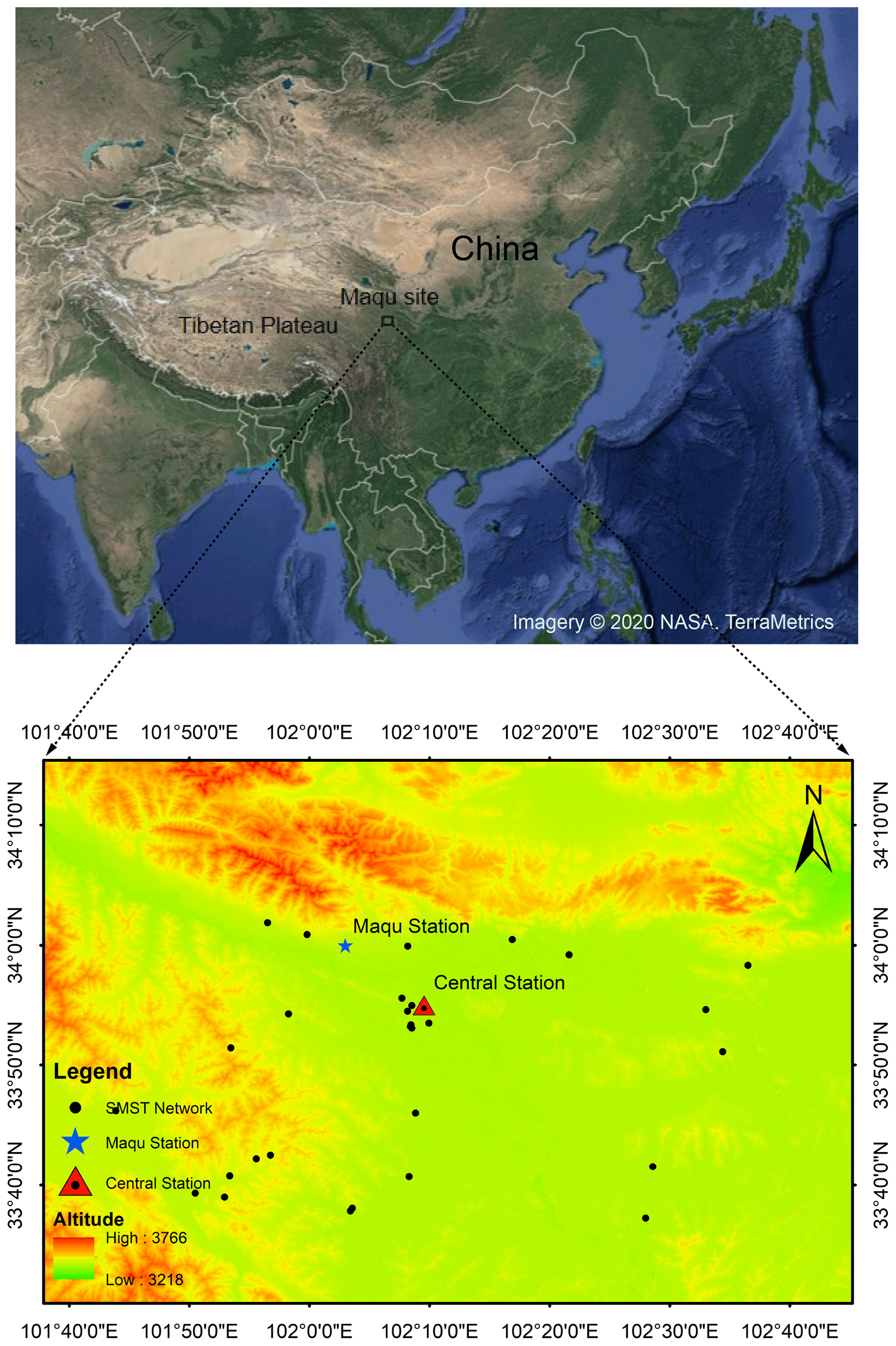
Figure 1Geographical location of Maqu soil moisture and temperature (SMST) monitoring network and the center station. © NASA TerraMetrics 2020
For this research, data from March 2016 to August 2018 collected at the central experimental site (33∘54′59′′ N, 102∘09′32′′, elevation: 3430 m) were utilized (see Fig. 1). Seasonally frozen ground is characteristic of this site, with the maximum freezing depth approaching around 0.8 m under current climate conditions. The dedicated SMST profile (central station; Fig. 1), with sensors installed at depths of 2.5, 5, 10, 20, 40, 60, and 100 cm, was used for validating the model simulations. Note that there are data gaps (25 March–8 June 2016 and 29 March–27 July 2017, extended to 12 August 2018 for 40 cm) due to the malfunction of instruments and the difficulty of maintaining the network under such harsh environmental conditions.
2.2 Data
2.2.1 Land surface energy and carbon fluxes and vegetation dynamics
Starting from the raw NEE (net ecosystem exchange) and ancillary meteorological data (friction velocity u∗, global radiation Rg, soil temperature Tsoil, air temperature Tair, and vapor pressure deficit, VPD), we employed the REddyProc package (Reichstein et al., 2005; Wutzler et al., 2018) as a postprocessing tool to obtain the time series of NEE, GPP (gross primary production), and ecosystem respiration Reco dynamics. Three different techniques, u∗ filtering, gap filling, and flux partitioning, were adopted in REddyProc package. The periods with low turbulent mixing were firstly determined and filtered for quality control (u∗ filtering; Papale et al., 2006). Then, considering the covariation of fluxes with meteorological variables and the temporal autocorrelation of fluxes, the marginal distribution sampling algorithm was used as the gap-filling method to replace the missing data (Reichstein et al., 2005). Three cases were identified according to the availability of Rg, Tair, and VPD: for case 1, Rg, Tair, and VPD data are available; for case 2, only Rg data are available; and for case 3, none of the Rg, Tair, and VPD data are available. A lookup table (LUT) method was used to search for similar meteorological conditions (i.e., under which Rg, Tair, and VPD do not deviate by more than 50 W m−2, 2.5 ∘C, and 5 hPa, respectively, for case 1) within a certain time window. The average value of NEE under these similar meteorological conditions was used to replace the missing gaps. The time window size started from 7 d and extended to 14 d if no similar meteorological conditions were detected. A similar LUT approach was utilized for case 2, and similar meteorological conditions were determined only by Rg within a time window of 7 d. For case 3, the missing value of NEE was replaced by the average value of adjacent hours (within 1 h) on the same day or at the same time of the day, which was derived from the mean diurnal course within 2 d. The aforementioned three steps were repeated with increased window sizes until the missing value could be properly filled. Finally, NEE was separated into GPP and Reco by nighttime-based and daytime-based approaches (Lasslop et al., 2010). Land surface energy fluxes (LE, H) were processed simultaneously using the aforementioned u∗ filtering and gap filling methods with the REddyProc package.
Furthermore, we downloaded MCD15A3H (Myneni et al., 2015) and MOD17A2H (Running et al., 2015) products for this site as the auxiliary ecosystem carbon and vegetation dynamics data from the Oak Ridge National Laboratory Distributed Active Archive Center (ORNL DAAC) website. MCD15A3H provides an estimation of 8 d composites of LAI (leaf area index) and FAPAR (fraction of absorbed photosynthetically active radiation), while MOD17A2H provides an 8 d composite of GPP (gross primary production). Both MODIS products are at a resolution of 500 m.
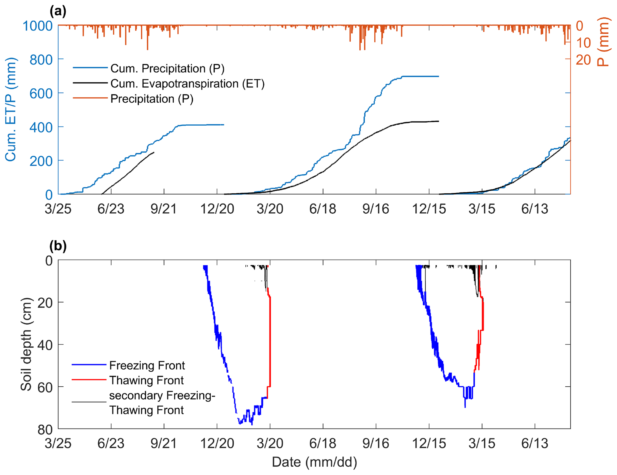
Figure 2(a) Observed cumulative precipitation (P) and evapotranspiration (ET) and (b) observed propagation of the freezing and thawing front, with blue, red, and black colors signifying the primary propagation of freezing front and thawing front (FF and TF) and the secondary freezing and thawing front (sFTF) occurring at top soil layers, respectively, for the period 25 March 2016–12 August 2018 at the Maqu site.
2.2.2 Precipitation, evapotranspiration, and frost front
The observed surface water conditions over the entire study period, including the precipitation and cumulative evapotranspiration (which is obtained by summing up the hourly latent heat flux measured by the eddy covariance system) are shown in Fig. 2a. Both ET and precipitation are low until the end of the freezing period (see Fig. 2b); during this early period, the daily average ET is 0.15 mm d−1. During the growing season, the cumulative precipitation increases and ET follows at a lower rate. The average daily ET for the entire observation period is 1.45 mm d−1.
Figure 2b presents the development of freezing depth with time. Several freezing and thawing cycles frequently occurred at the beginning of the winter, which initializes the freezing and thawing processes. The freezing front started to propagate at an average rate of 1.34 and 0.86 cm d−1, reaching its maximum depth at around 80 and 70 cm for the years 2016–2017 and 2017–2018, respectively. Then the thawing process was activated by the atmospheric forcing at the surface and subsurface soil heat flux at the bottom of the soil.
3.1 T&C model (unCPLD)
The Tethys–Chloris model (T&C) (Fatichi et al., 2012b) simulates the dynamics of energy, water, and vegetation and has been successfully applied to a very large spectrum of ecosystems and environmental conditions (Fatichi and Ivanov, 2014; Fatichi et al., 2016b; Pappas et al., 2016; Fatichi and Pappas, 2017; Mastrotheodoros et al., 2017). The model simulates the energy, water, and carbon exchanges between the land surface and the atmospheric surface layer, accounting for aerodynamic, undercanopy, and leaf boundary layer resistances, as well as for stomatal and soil resistance. The model further describes vegetation physiological processes including photosynthesis, phenology, carbon allocation, and tissue turnover. Dynamics of water content in the soil profile in the plot-scale version are solved using the one-dimensional (1-D) Richards equation. Heat transfer in the soil is solved by means of the heat diffusion equation. Soil heat and water dynamics are uncoupled (however, note that T&C is termed unCPLD to distinguish it later from the coupling with STEMMUS). The detailed model description is provided in the above-mentioned references, and some key elements applied for this study are explained in the following.
The T&C model uses the 1-D Richards equation, which describes the water flow under gravity and capillary forces in isothermal conditions for variably saturated soils:
where θ (m3 m−3) is the volumetric water content; q (kg m−2 s−1) is the water flux; z (m) is the vertical direction coordinate; S (kg m−3 s−1) is the sink term for transpiration and evaporation fluxes; ρL (kg m−3) is the liquid water density; K (m s−1) is the soil hydraulic conductivity; ψ (m) is the soil water potential; and t (s) is the time. In T&C, the nonlinear partial differential equation is solved using a finite volume approach with the method of lines (MOL) (Lee et al., 2004). MOL discretizes the spatial domain and reduces the partial differential equation to a system of ordinary differential equations in time, which can be expressed as follows:
where dz,i (m) is the thickness of layer i; qi (m s−1) is the vertical outflow from a layer i; Tv (m s−1) is the transpiration fluxes from the vegetation; rv,i is the fraction of root biomass contained in soil layer i; Ebare (m s−1) is evaporation from the bare soil; and Es (m s−1) is evaporation from soil under the canopy.
The heat conservation equation used in the T&C neglects the coupling of water and heat transfer physics, and only the heat conduction component is considered, which can be expressed as follows:
where ρsoil (kg m−3) is the bulk soil density; Csoil (J kg−1 K−1) is the specific heat capacities of bulk soil; and λeff (W m−1 K−1) is the effective thermal conductivity of the soil. T (K) is the soil temperature. When soil undergoes freezing and thawing processes, the latent heat flux due to water phase change becomes important, which is not considered in the original T&C model, but it is in the T&C-FT (freezing and thawing) model.
3.2 T&C-FT model (unCPLD-FT)
To account for frozen soil physics, the T&C-FT model considers the ice effect on hydraulic conductivity, thermal conductivity, heat capacity, and subsurface latent heat flux. However, the vapor flow and the thermal effect on water viscosity are not considered in T&C-FT, and during the non-frozen period, soil water and heat are still independently transferred as in T&C (this version is here named unCPLD-FT). To explicitly account for freezing and thawing processes, the heat conservation equation is written as follows:
where the latent heat associated with the freezing and thawing processes is explicitly considered, and ice water content θice is a prognostic variable, which is simulated along with liquid water content for each soil layer. Specifically, when Eq. (4) is rewritten in terms of an apparent volumetric heat capacity Capp (Hansson et al., 2004; Gouttevin et al., 2012), it can be solved equivalently to Eq. (3):
where Capp can be computed knowing the temperature T (K), latent heat of fusion Lf, and the differential (specific) water capacity dθ∕dψ at a given liquid water content θ (Hansson et al., 2004):
The effective thermal conductivity λeff (W m−1 K−1) and the specific soil heat capacity Csoil (J kg−1 K−1) are computed accounting for solid particles, water, and ice content (Johansen, 1975; Farouki, 1981; Lawrence et al., 2018; Yu et al., 2018). The soil freezing characteristic curve providing the liquid water potential in frozen soil is computed following the energy conservative solution proposed by Dall'Amico et al. (2011), and it can be combined with various soil hydraulic parameterizations including van Genuchten (1980) and Saxton and Rawls (2006) to compute the maximum liquid water content at a given temperature and consequently ice and liquid content profiles at any time step (Fuchs et al., 1978; Yu et al., 2018).
Finally, saturated hydraulic conductivity is corrected in the presence of ice content (e.g., Hansson et al., 2004; Yu et al., 2018). Note that beyond latent heat associated with phase change and changes in thermal and hydraulic parameters because of ice presence, all the other soil physics processes described by STEMMUS are not considered here, and heat and water fluxes are still not entirely coupled in T&C-FT.
3.3 STEMMUS model
The Simultaneous Transfer of Energy, Mass and Momentum in Unsaturated Soil (STEMMUS) model solves soil water and soil heat balance equations simultaneously in one time step (Zeng et al., 2011a, b; Zeng and Su, 2013). The Richards equation with modifications made by Milly (1982) is utilized to mimic the coupled soil mass and energy transfer process. The vapor diffusion, advection, and dispersion are all taken into account as water vapor transport mechanisms. The root water uptake process is regarded as the sink term of soil water and heat balance equations, building up the linkage between soil and atmosphere (Yu et al., 2016). In STEMMUS, temporal dynamics of three phases of water (liquid, vapor, and ice) are explicitly presented and simultaneously solved by spatially discretizing the corresponding governing equations of liquid water flow and vapor flow.
where ρV and ρice (kg m−3) are the density of water vapor and ice, respectively; θL, θV, and θice (m3 m−3) are the soil liquid, vapor, and ice volumetric water content, respectively; qLh and qLT (kg m−2 s−1) are the soil liquid water flow driven by the gradient of soil matric potential and temperature , respectively; qVh and qVT (kg m−2 s−1) are the soil water vapor fluxes driven by the gradient of soil matric potential and temperature , respectively; DTD (kg m−1 s−1 K−1 is the transport coefficient of the adsorbed liquid flow due to temperature gradient; DVh (kg m−2 s−1) is the isothermal vapor conductivity; and DVT (kg m−1 s−1 K−1) is the thermal vapor diffusion coefficient.
STEMMUS takes into account different heat transfer mechanisms, including heat conduction (), convective heat transferred by liquid and vapor flow, the latent heat of vaporization (ρVθVL0), the latent heat of freezing and thawing (−ρiceθiceLf), and a source term associated with the exothermic process of the wetting of a porous medium (integral heat of wetting) ().
where ρs (kg m−3) is the soil solids density; θs is the volumetric fraction of solids in the soil; Cs, CL, CV, and Cice (J kg−1 K−1) are the specific heat capacities of soil solids, liquid, water vapor, and ice, respectively; Tref (K) is the arbitrary reference temperature; L0 (J kg−1) is the latent heat of vaporization of water at the reference temperature; Lf (J kg−1) is the latent heat of fusion; W (J kg−1) is the differential heat of wetting (expressed by Edlefsen and Anderson, 1943, as the amount of heat released when a small amount of free water is added to the soil matrix); and qL and qV (kg m−2 s−1) are the liquid and vapor water flux, respectively. Additional details on the equations for solving the coupled water and heat equations can be found in Zeng et al. (2011a, b) and Zeng and Su (2013). In the Appendix, a notation table summarizes the above equations.
3.4 Coupling T&C and STEMMUS (CPLD)
As mentioned above (Sect. 3.1–3.2), T&C considers soil water and heat dynamics independently, and T&C-FT only considers ice effects associated with latent heat and thermal and hydraulic parameters, while all other soil physics processes of STEMMUS are not considered. On the other hand, while the STEMMUS model can reproduce well the soil water and heat transfer process in frozen soil, it lacks a detailed description of land surface processes and of the ecohydrological feedback mechanisms. To take advantage of the strengths of both models, we coupled the STEMMUS model with the land surface and vegetation components of the T&C model (termed CPLD) to better describe the soil–plant–atmosphere continuum (SPAC) in cold regions.
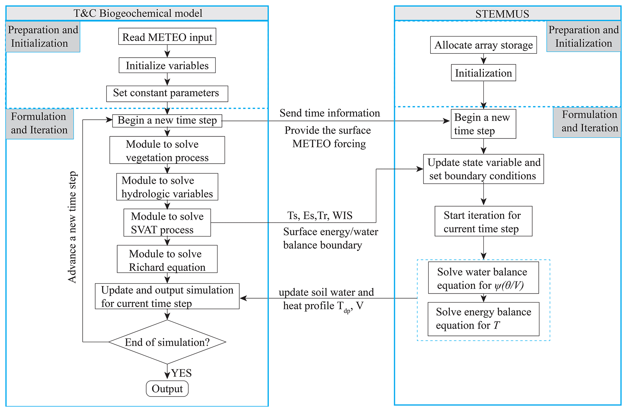
Figure 3Coupling procedure of the STEMMUS and T&C models. METEO is the meteorology forcing, and SVAT is acronym for the soil–vegetation–atmosphere mass and heat transfer. Ts, Es, Tr, and WIS are the surface temperature, soil evaporation, plant transpiration, and incoming water flux to the soil, respectively. Tdp and V are the soil profiles of temperature (in ∘C) and liquid water volume in each layer (mm).
The current coupling procedure between the STEMMUS and the T&C models is based on a sequential coupling via the exchange of mutual information within one time step (see Fig. 3). The T&C model and STEMMUS model run sequentially within one time step. First, the preparation and initialization modules are called. Meteorology inputs and constant parameters are set, and the initialization process is performed. After the inputs are prepared, the main iteration process starts. T&C is in charge of the time control information (starting time, time step, elapsed time) and informs the STEMMUS model with these time settings every time step. Meanwhile, the surface boundary conditions obtained by the solution of vegetation and land surface energy dynamics are also sent to drive the STEMMUS model. The surface latent heat flux (LE) is partitioned into soil evaporation (used for setting the surface boundary condition of soil water flow) and plant transpiration (further subdivided into layer-specific root water uptakes representing the sink terms of Richards equation).
After convergence is achieved in the soil module (i.e., convergence criteria is set to 0.001 for both soil matric potential, in centimeters, and soil temperature, in kelvin), STEMMUS estimates soil temperature and soil moisture (hereafter ST/SM) profiles, which are utilized to update ST/SM states in the T&C model. The T&C model then utilizes this updated ST/SM information (rather than its own computed ST/SM profiles) to proceed with the ecohydrological simulations in the following time step. Such iterations continue till the end of the simulation period.
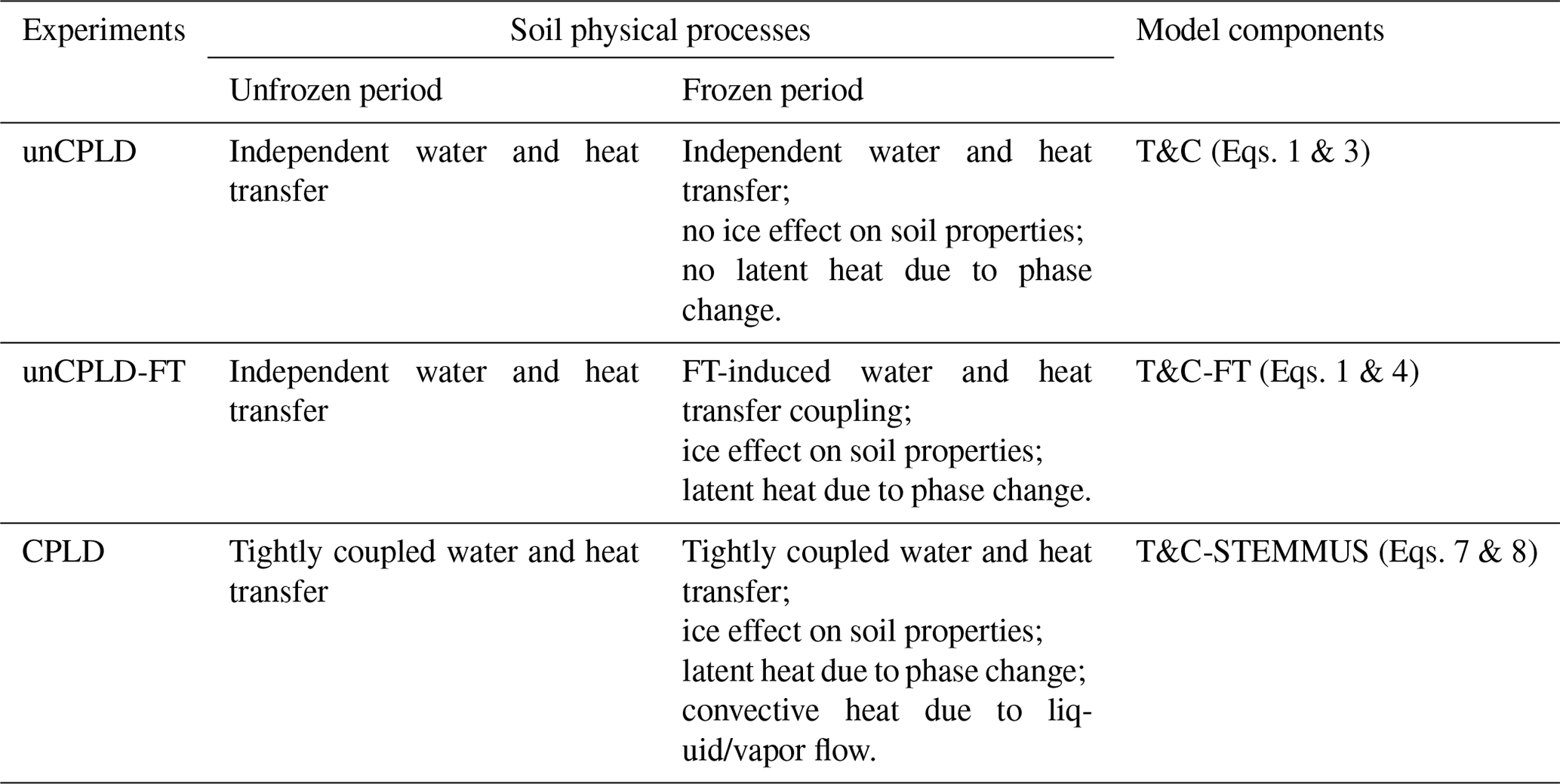
Table 1Numerical experiments with various mass and energy transfer processes.
Note:
Independent water and heat transfer: soil water and heat transfer process is
independent.
FT-induced water and heat transfer coupling: soil water and heat transfer
process is coupled only during the freezing and thawing (FT) periods. Soil water
flow is affected by temperature only through the presence of soil ice
content (the impedance effect).
Tightly coupled water and heat transfer: soil water and heat transfer
process is tightly coupled; vapor flow, which links the soil water and heat
flow, is taken into account; thermal effect on water flow is considered (the
hydraulic conductivity and matric potential is dependent on soil
temperature; when soil freezes, the hydraulic conductivity is reduced by the
presence of soil ice, which is temperature dependent); and the
convective/advective heat due to liquid/vapor flow can be calculated.
Ice effect on soil properties: the explicit simulation of ice content and
its effect on the hydraulic/thermal properties.
3.5 Numerical experiments
To investigate the role of the increasing complexity of vadose zone physics in ecosystem functioning, three numerical experiments were designed on the basis of the aforementioned modeling framework (Table 1). For the first experiment, the original T&C model was run alone and termed unCPLD simulation. For the unCPLD model, soil water and heat transfer are independent with no explicit consideration of soil ice effect. For the second experiment, the updated T&C model with explicit consideration of freezing and thawing processes was run as it can estimate the dynamics of soil ice content and the related effect on water and heat transfer (e.g., blocking effect on water flow, heat release/gain due to phase change) but is otherwise exactly equal to the original T&C model. This second simulation is named the unCPLD-FT simulation, in which the term unCPLD generally refers to the fact that the T&C model and STEMMUS model are not yet coupled. For the third experiment, the STEMMUS model was coupled with the T&C model to enable not only frozen soil physics but also additional processes and most importantly the tight coupling of water and heat effects. This simulation is named the CPLD simulation. In this third scenario, vapor flow, which links the soil water and heat flow, is explicitly considered. In addition to the ice blocking effect as presented in unCPLD-FT, the thermal effect on water flow is also expressed with the temperature dependence of hydraulic conductivity and matric potential. Furthermore, not only the latent heat due to phase change but also the convective heat due to liquid/vapor flow are also simulated.
Hourly meteorological forcing (including downwelling solar and thermal radiation, precipitation, air temperature, relative humidity, wind speed, and atmospheric pressure) was utilized to drive the models. For the adaptive time step of the STEMMUS simulation, the linear interpolation between two adjacent hourly meteorological measurements was used to generate the required values at every second. The hydrological related initial states, e.g., initial snow water equivalent and soil water and temperature profiles, were taken as close as possible to the observed ones. Since the current initial conditions of the carbon and nutrient pools in the soil are unknown, we spin-up carbon and nutrient pools, running only the soil biogeochemistry module for 1000 years using average climatic conditions and prescribed litter inputs taken from preliminary simulations. Then we used the spun-up pools as initial conditions for the hourly scale simulation over the period for which hourly observations are available. This last operation is repeated two times, which allows a dynamic equilibrium of nutrient and carbon pools in the soil and vegetation to be reached.
The total depth of the soil column was set to 3 m and divided into 18 layers with a finer discretization in the upper soil layers (1–5 cm) than that in the lower soil layers (10–50 cm). Soil samples were collected and transported to the laboratory to determine the soil hydrothermal properties (see Zhao et al., 2018, for detail). The average soil texture and fitted van Genuchten parameters at three soil layers were listed in Table S1 in the Supplement. Vegetation parameters were obtained on the basis of the literature and expert knowledge (see a summary of the adopted vegetation parameters in Table S2). All three numerical experiments shared the same soil and vegetation parameter settings.
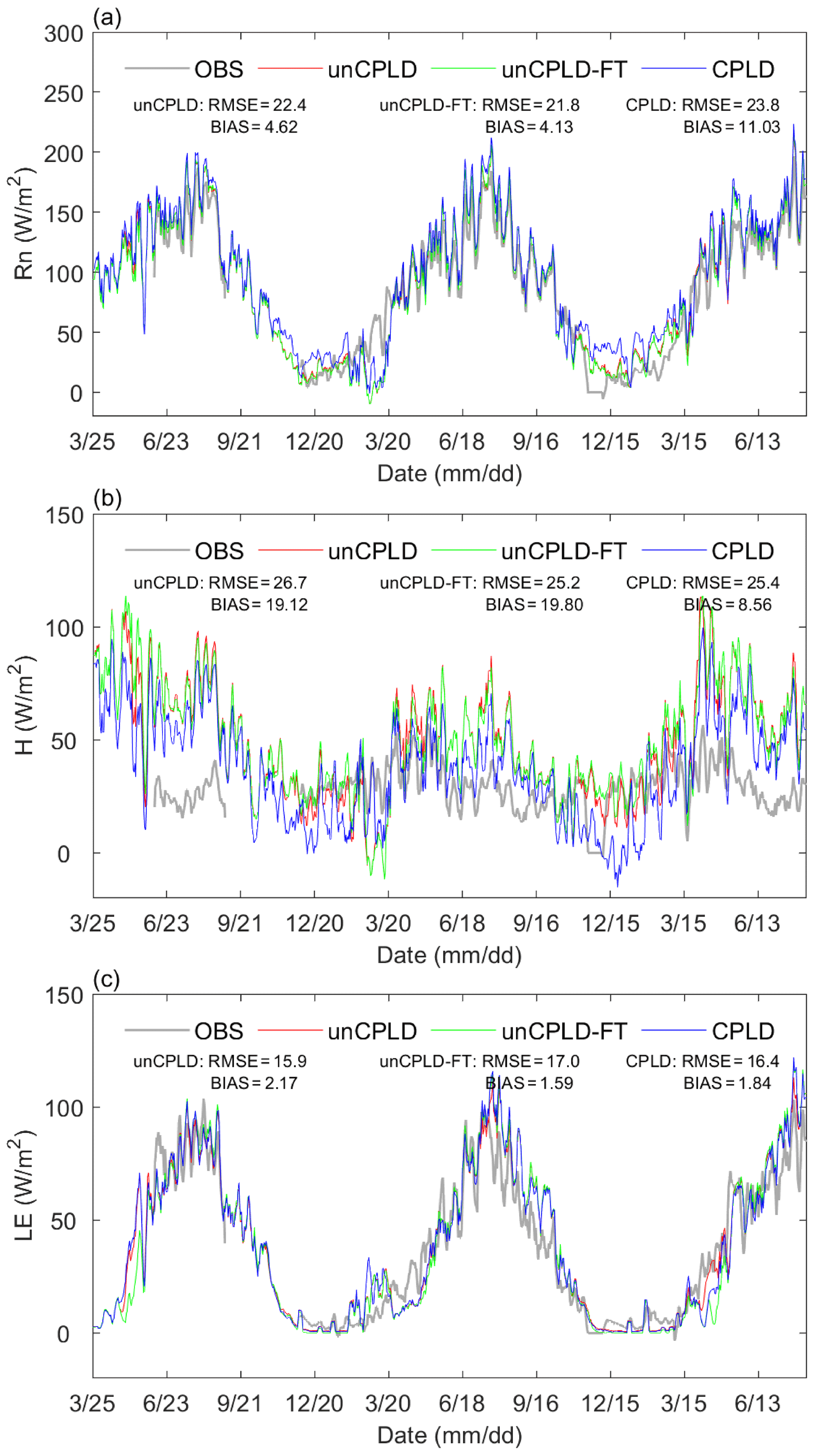
Figure 4Comparison of observed and simulated 5 d moving average dynamics of net radiation (Rn), latent heat flux (LE), and sensible heat flux (H) using the original (uncoupled) T&C (unCPLD), T&C with consideration of the FT process (unCPLD-FT), and coupled T&C and STEMMUS (CPLD) models.
4.1 Surface flux simulations
The 5 d moving average dynamics of the net incoming radiation (Rn), latent heat (LE), and sensible heat (H) fluxes measured and simulated by the unCPLD, unCPLD-FT, and CPLD models for the study period are presented in Fig. 4. The seasonality and magnitude of surface fluxes can be captured across seasons. A good match between observed and simulated Rn and LE was identified during the whole period with isolated observable discrepancies (Figs. 4a, c, and S1). Compared to unCPLD and unCPLD-FT simulations, the CPLD model simulated similar dynamics of LE, while it generally produced a larger overestimation of Rn, especially during the frozen period. These mismatches of Rn can be partly attributed to the uncertainties of observed winter precipitation events and the following snow cover dynamics, which might not be captured well in the models. For the sensible heat flux simulations, all three models can reproduce the seasonal dynamics. However, an overestimation of the 5 d average values was observed in several periods. Given the good correspondence between observations and simulations of net radiation and latent heat, this discrepancy might be a model shortcoming due to the simplification in considering only one single surface prognostic temperature (i.e., soil surface and vegetation surface temperature were assumed to be the same), but it can also be caused by the lack of energy balance closure in the eddy covariance data (see Sect. 4.5). Compared to unCPLD and unCPLD-FT simulations, the overestimation was reduced in the CPLD model simulations, and the H dynamics were closer to observations during the growing season.

Figure 5Scatter plots of observed and model-simulated daily average surface fluxes (net radiation: Rn; latent heat: LE; and sensible heat flux: H) using the original (uncoupled) T&C (unCPLD), T&C with consideration of the FT process (unCPLD-FT), and coupled T&C and STEMMUS (CPLD) models, with the color indicating the frequency of surface flux values.
The correlation between observed and simulated daily average surface heat fluxes with the unCPLD, unCPLD-FT, and CPLD models is shown in Figs. 5, S2, and S3. Noticeably, all the unCPLD/CPLD model scenarios, with different water and heat transfer physics, exhibited nearly identical statistical performance of surface flux simulations (Fig. 5). The overall performance of the model in terms of turbulent flux simulations can be regarded as acceptable given the uncertainties in winter precipitation and eddy covariance observations in such a challenging environment even though discrepancies exist during certain periods (Fig. 4).
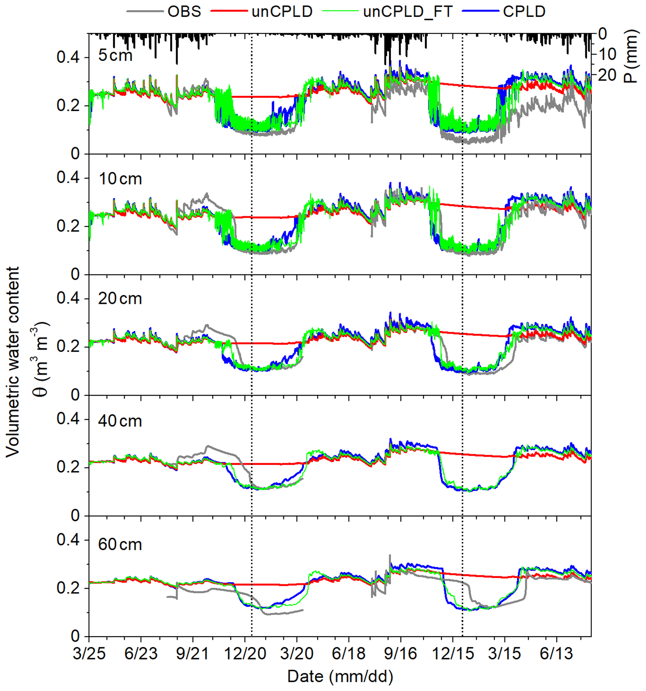
Figure 6Measured and estimated soil moisture at various soil layers using uncoupled T&C (unCPLD), uncoupled T&C with the FT process (unCPLD-FT), and coupled T&C and STEMMUS (CPLD) models. Note that in unCPLD model, soil ice content is not explicitly considered, and thus all the water remains in a liquid phase, which leads to a strong overestimation of winter soil water content in frozen soils.
4.2 Soil moisture and soil temperature simulations
The capability of the three models to reproduce the temporal dynamics of soil moisture is illustrated in Fig. 6. By explicitly considering soil ice content, the unCPLD-FT and CPLD models captured well the response of soil moisture dynamics to the freeze–thaw cycles, while the unCPLD model lacked such a capability and maintained a higher soil water content throughout the winter period but a slightly lower water content in the growing season. For all three models, the consistency between the measured and simulated soil water content at five soil layers was satisfactory during the growing season, indicating the models' capability in portraying the effect of precipitation and root water uptake on the soil moisture conditions.
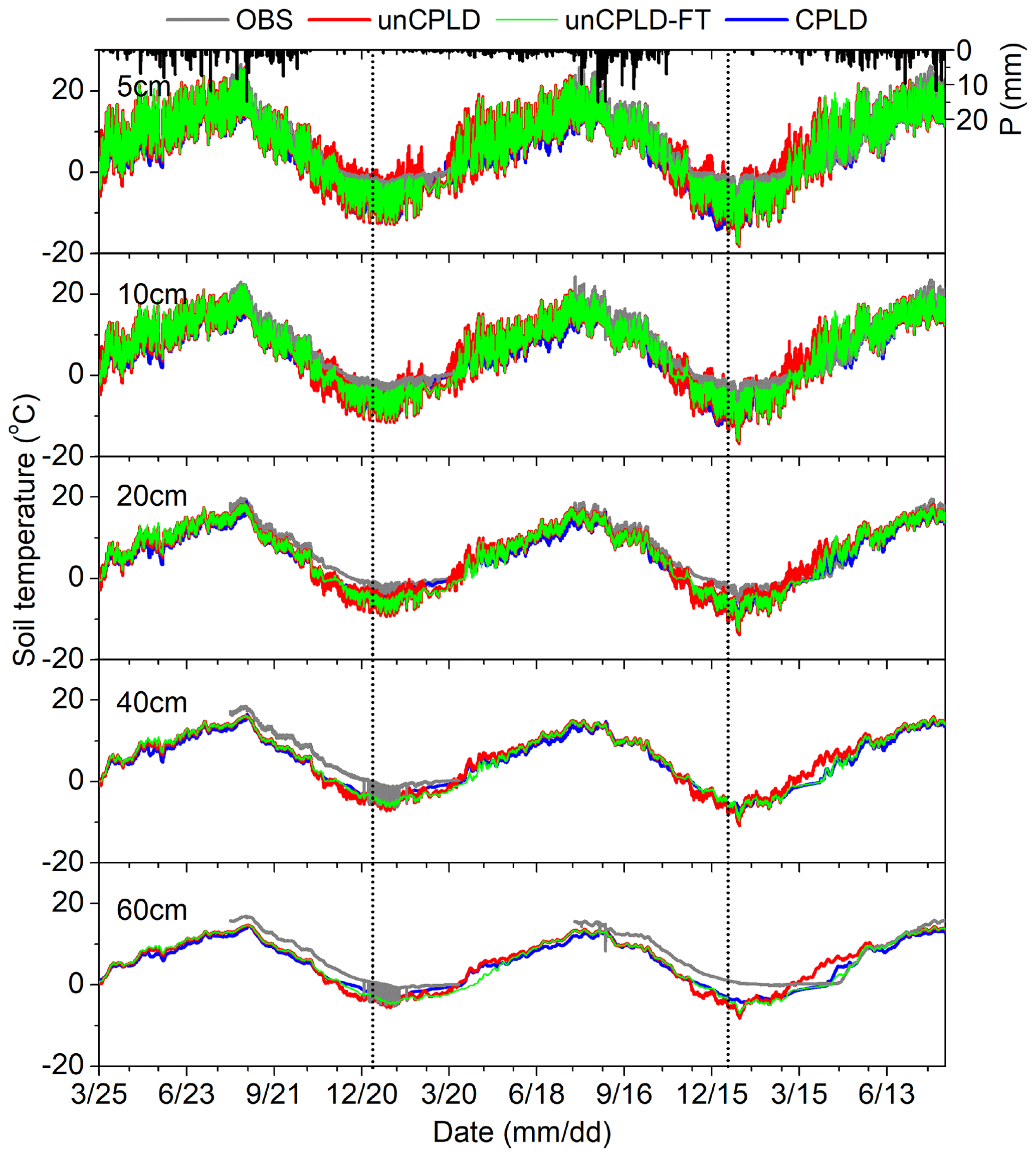
Figure 7Measured and simulated soil temperature at various soil layers using uncoupled T&C (unCPLD), T&C with the FT process (unCPLD-FT), and coupled T&C and STEMMUS (CPLD) models.
Five layers of soil temperature measurements were employed to test the performance of the model in reproducing the soil temperature profiles (Fig. 7). During the growing period, all three models can capture the dynamics of soil temperature well. In this period, there is no significant difference among the three models in the magnitude and temporal dynamics of soil temperature. During the freezing period, a general underestimation of soil temperature and overestimation of its diurnal fluctuations were found at shallower soil layers, which may indicate that there is some thermal buffering effect in reality not fully captured in the models. Compared to the unCPLD-FT and CPLD models, the unCPLD model simulations had stronger diurnal fluctuations of soil temperature with an underestimation of temperature at the beginning of the freezing period and a considerable overestimation during the thawing phase. This results in an earlier date passing the 0 ∘C threshold than in the unCPLD-FT and CPLD simulations. It should be noted that for the deeper soil layers (e.g., 60 cm in Fig. 7), all models tended to simulate the early start of freezing soil temperatures and considerably underestimated the soil temperature during the frozen period. This can be due to the uncertainties in soil organic layer parameters, the not fully captured snow cover effect (Gouttevin et al., 2012), a potentially pronounced heterogeneity in soil hydrothermal properties, or the potential role of solutes on the freezing-point depression (as the presence of solute lowers the freezing soil temperature) (Painter and Karra, 2014). These mismatches in deep soil temperature degraded the model performance in simulating the dynamics of liquid water (Fig. 6) and ice content (Fig. 8) during the frozen period.
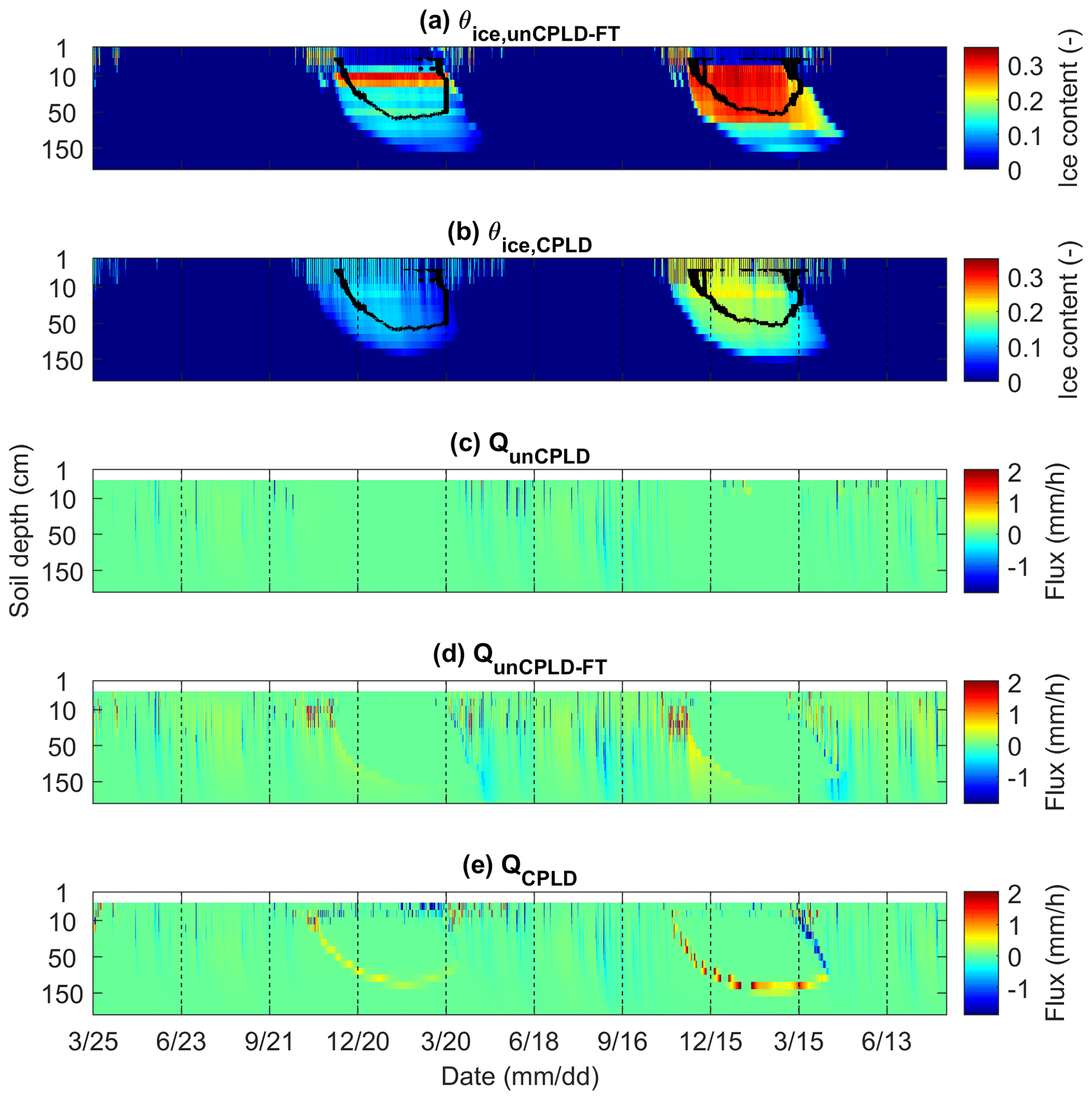
Figure 8Soil ice content from (a) unCPLD-FT and (b) CPLD model simulations with freezing front propagation derived from the measured soil temperature and vertical water flux (positive value indicates upward water flow) from (c) unCPLD, (d) unCPLD-FT, and (e) CPLD model simulations. Note that soil ice content is not represented in the unCPLD model and the fluxes in the top 2 cm soil layers were not reported to highlight fluxes in the lower layers.
4.3 Soil ice content and water flux
The time series of soil ice content and water flux from the unCPLD, unCPLD-FT, and CPLD model simulations for soil layers below 2 cm are presented in Fig. 8. As soil ice content measurements were not available, the freezing front propagation inferred from the soil temperature measurements was employed to qualitatively assess the model performance. The phenomenon that a certain amount of liquid water flux moves upwards along with the freezing front can be clearly noticed for both the unCPLD-FT and CPLD model simulations. As the soil matric potential changes sharply during the water phase change, a certain amount of water fluxes will be forced towards the phase changing region, a phenomenon known as cryosuction. Such a phenomenon has already been demonstrated from theoretical and experimental perspectives by many researchers (Hansson et al., 2004; Watanabe et al., 2011; Yu et al., 2018, 2020). Cryosuction is much more accentuated in the unCPLD-FT simulation, while it is of course absent in the unCPLD model simulations (Fig. 8c). Precipitation-induced downward water flux can be observed in all models during summer with very similar patterns. It is of note that compared to the unCPLD-FT model, the CPLD model presented a relatively lower presence of soil ice content, while its temporal dynamics were closer to the observed freezing and thawing front propagation. The difference between the two simulations can be attributed to the constraints imposed by the interdependence of liquid, ice, and vapor in the soil pores which is considered only in the CPLD model.
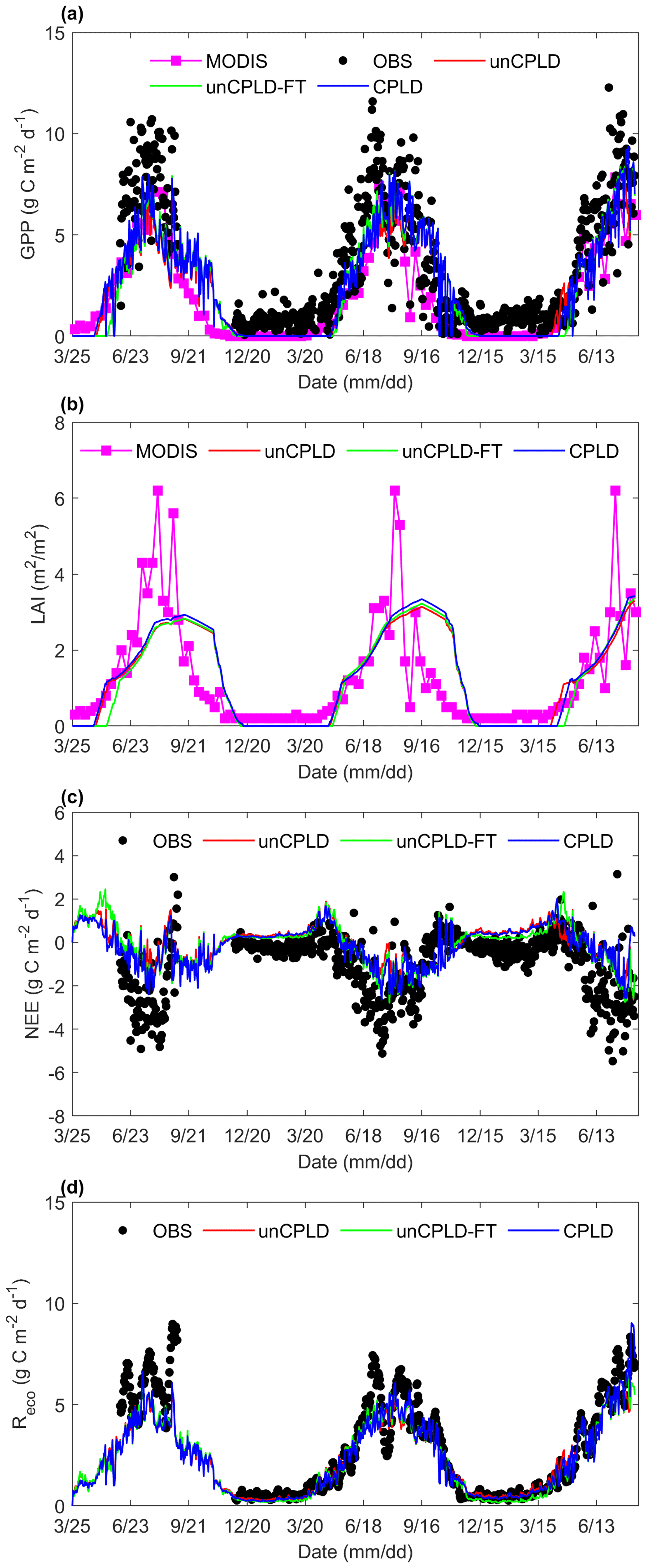
Figure 9Comparison of observations from eddy covariance (OBS) or MODIS remote sensing and simulated (a) gross primary production (GPP), (b) leaf area index (LAI), (c) net ecosystem exchange (NEE), and (d) ecosystem respiration (Reco) using the unCPLD, unCPLD-FT, and CPLD models. MODIS refers to the data from MODIS-GPP and MODIS LAI products.
4.4 Simulations of land surface carbon fluxes
The eddy-covariance-derived vegetation productivity and remote sensing (MODIS) observations of vegetation dynamics are compared with the model simulation in Fig. 9. When compared with in situ eddy covariance observations, slightly earlier growth and considerably earlier senescence of grassland with lower photosynthesis were inferred from the MODIS GPP product (Fig. 9a). The mismatch in the phenology is likely a combined issue of 8 d (or longer if clouds are impeding the view) composites of MODIS products and of the challenge of translating vegetation reflectance signals into productivity or leaf area index (LAI) during the grass senescent phase.
Taking eddy covariance observations as the reference, the onset date of grassland appears to be captured well by both unCPLD and CPLD model simulations, while there is a delayed onset date in the unCPLD-FT model. Leaf senescence and dormancy phase are a bit delayed in the models when compared with eddy covariance data and considerably delayed when compared to MODIS LAI even though the latter is particularly uncertain, as described above. Although there is an observable underestimation of GPP compared to the eddy covariance measurements, the dynamics of GPP, which is mainly constrained by the photosynthetic activity and environmental stresses, are reasonably reproduced by all model simulations.
The underestimation of GPP has magnified consequences in terms of reproducing NEE dynamics by the unCPLD and CPLD models. While this might be seen as a model shortcoming, there are a number of reasons that lead to questioning the reliability of the magnitude of carbon flux measurements at this site. By checking other ecosystems' productivity under similar conditions, the annual average GPP for the Tibetan Plateau meadow ecosystem ranges from 300 to 935 g C m−2 yr−1, while the annual average NEE ranges from −79 to −213 g C m−2 yr−1 (see the literature summary in Table S3). The EC system used in this experimental site observes an annual GPP and NEE of 1132.52 and −293.24 g C m−2 yr−1. Both the GPP and NEE measured fluxes are significantly larger than existing estimates of the carbon exchange for such an ecosystem type and are unlikely to be correct in absolute magnitude. The ecosystem respiration (Reco), indicating the respiration of activity of all living organisms in an ecosystem, is shown in Fig. 9d. The performance of all three model simulations in reproducing Reco dynamics can be characterized as having an overall good match with regards to the magnitude and seasonal dynamics, which further suggests the discrepancy in observed/simulated GPP is the driver of the disagreement in NEE.
The difference in the soil liquid water and temperature profile simulations between the CPLD and unCPLD models (as shown in Figs. 6 and 7) resulted in differences in simulated vegetation dynamics, especially concerning the leaf onset date, which is affected by integrated winter soil temperatures. The unCPLD-FT model has a delay in the vegetation onset date when compared to other simulations due to the significant cryosuction that prolongs freezing conditions and keeps lower soil temperatures. This makes the unCPLD simulation have a slightly shorter active vegetation season compared to the CPLD model simulations. The lower GPP in the unCPLD simulations is instead related to a slightly enhanced water stress induced by the different soil moisture dynamics during the winter and summer seasons with a lower root zone moisture produced by the unCPLD model (Fig. 6), which affects the plant photosynthesis and growth. Differences in soil temperature profiles can also affect root respiration in generating additional small differences in GPP.
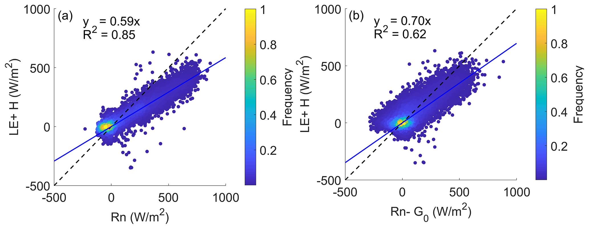
Figure 10Scatter plots of eddy-covariance-measured hourly values of LE+H versus (a) Rn and (b) Rn−G0 with the color indicating the occurrence frequency of surface flux values. G0, the ground heat flux, was estimated by the CPLD model.
4.5 Surface energy balance closure
The energy balance closure problem, usually identified because the sum of latent (LE) and sensible (H) heat fluxes is less than the available energy (Rn−G0), is quite common in eddy covariance measurements (Su, 2002; Wilson et al., 2002; Leuning et al., 2012). The energy imbalance of EC measurements is particularly significant at sites over the Tibetan Plateau (Tanaka et al., 2003; Yang et al., 2004; Chen et al., 2013; Zheng et al., 2014). Figure 10 presents the energy imbalance of hourly LE and H by the eddy covariance measurements, observed Rn by the four-component radiation measurements, and the estimated ground heat flux (G0) by the CPLD model. The sum of measured LE and H was significantly less than Rn with the slope of LE+H versus Rn equal to 0.59 (Fig. 10a). Usually, the measurements of radiation are reliable (Yang et al., 2004). If we assume that the turbulence flux (LE, H) measurements are accurate, then the rest of the energy (around 41 % of Rn) should theoretically be consumed by ground heat flux G0, which is clearly impossible. When compared to the available energy (Rn−G0), the slope was increased to 0.70 (Fig. 10b). Table 2 demonstrates that the energy imbalance problem was significant across all seasons. The seasonal variation in energy closure ratio (ECR) can be identified for the case of LE+H versus Rn−G0, similar to the research of Tanaka et al. (2003), i.e., a good energy closure during the pre-monsoon periods while a degraded one during the summer monsoon periods.
These problems clearly suggest that care should be taken with the mutual data corroboration issue. Nevertheless, such an issue does not affect the comparison results among models with different vadose zone physics since we did not force any parameter calibration or data-fitting procedure but simply relied on physical constraints, the literature, and expert knowledge to assign model parameters.
Table 2Monthly values of energy closure ratio derived from eddy-covariance-measured LE+H versus Rn and Rn−G0, respectively (December 2017–August 2018). G0, the ground heat flux, was estimated by the CPLD model.

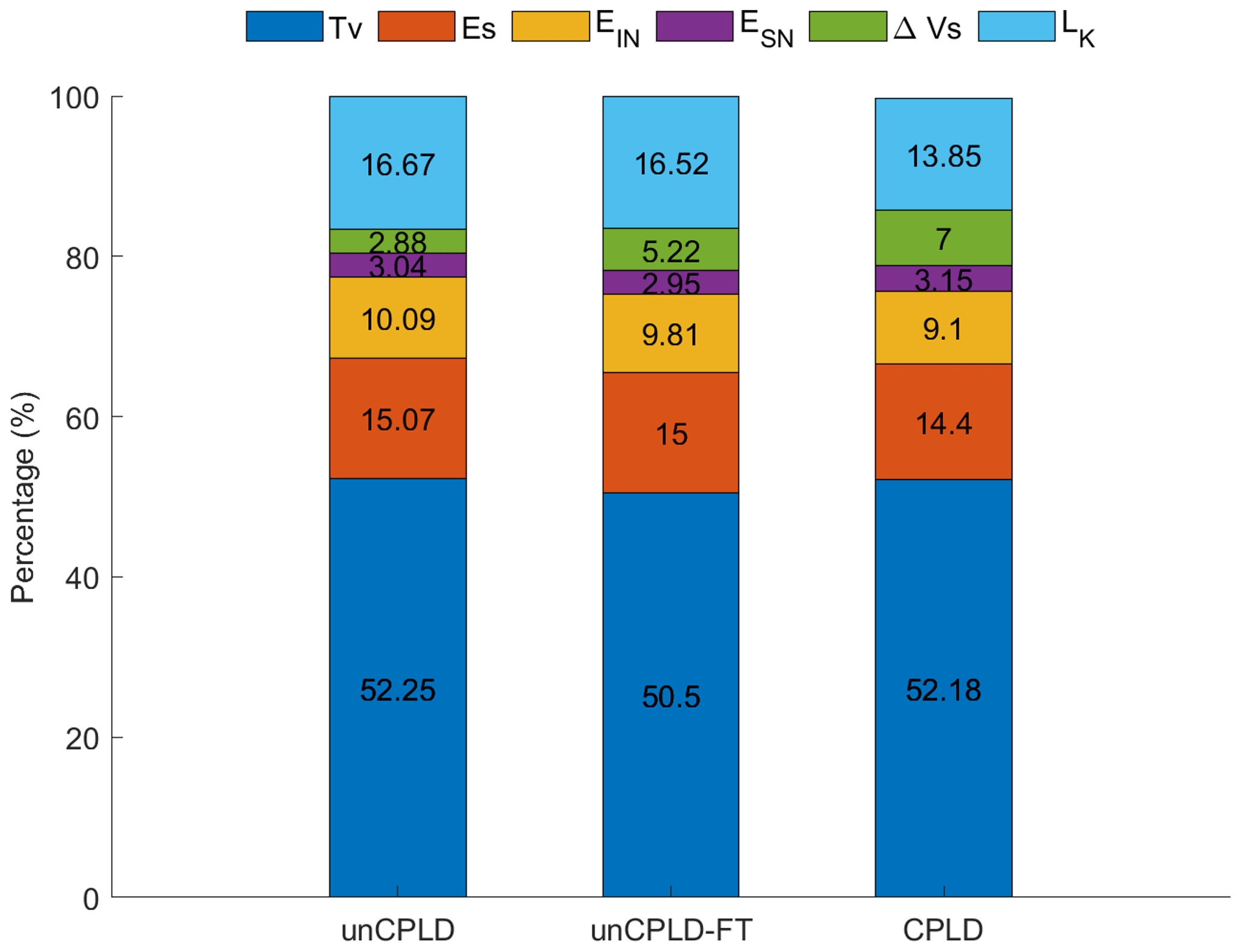
Figure 11Comparison of the relative ratios of different water budget components to precipitation during the whole simulation period produced by different model scenarios. Tv is transpiration, Es is surface evaporation, EIN and ESN are evaporation from intercepted canopy water and snow cover, ΔVs is changes in soil water storage, and LK is deep leakage water.
4.6 Effects on water budget components
The effect of different model versions on soil water budget components is illustrated in Fig. 11. The T&C model can describe in detail different water budget components. Precipitation can be partitioned into vegetation interception, surface runoff, and infiltration. Infiltrated water can then be used for surface evaporation (Es), root water uptake (i.e., transpiration, Tv), and changes in soil water storage (ΔVs). The other evaporation components, i.e., evaporation from intercepted canopy water (EIN) and snow cover (ESN), can be further distinguished by the T&C model. A certain amount of water will drain below the bottom of the 3 m soil column as deep leakage (LK).
All models demonstrated that most of the precipitation is used by ET. Less water was consumed by ET from unCPLD-FT simulations than that from unCPLD. This is due to the lower amount of vegetation transpiration (Tv) and intercepted canopy water evaporation (EIN) regulated by cooler late winter temperatures and the late beginning of the active vegetation season. The cooler late winter temperatures from unCPLD-FT simulations can be attributed to the retardation of the thawing process due to the phase-change-induced heat absorption and the soil-ice-induced modification of bulk heat capacity during the freezing and thawing transition period, which dampened the magnitude of temperature variations and delayed the thawing process. With explicit consideration of soil ice, hydraulic conductivity is also reduced, and vertical water flow is retarded during the frozen period (Kurylyk and Watanabe, 2013). This explains the higher value of ΔVs in the unCPLD-FT simulation (5.2 %) than that in the unCPLD simulation (2.8 %). Furthermore, at the end of the freezing period, the unCPLD-FT simulation presents a delayed vegetation onset and thus a decrease in ecosystem water consumption, which favors percolation toward deeper layers and the bottom leakage. Such a positive effect on the bottom leakage flux was slightly weaker than the negative effect (impeded water flow) due to frozen soil throughout the winter season. These results indicate that the presence of seasonally frozen soil can mediate the water storage in the vadose zone via both hydrological and plant physiological controls.
The effect of coupled water and heat physics (unCPLD vs. CPLD model) on the water budget components can be summarized as follows. (i) The amount of ecosystem water consumption (ET) was reduced due to the dampened surface evaporation process (evaporation from the soil surface and intercepted water). (ii) The water storage amount in the vadose zone increased, while the bottom leakage decreased. We attribute this to the way ice content is simulated in the CPLD simulation and also to the temperature dependence of soil hydraulic conductivity (see Table 1 and Supplement S1). Specifically, the high accumulation of ice content in the unCPLD-FT simulations indicates a relatively stronger cryosuction effect than in CPLD simulations. This cryosuction effect is mitigated in the fully coupled model because of water vapor transfer and thermal gradients even though different solutions in the parameterization of bulk soil thermal conductivity and volumetric soil heat capacity could also be responsible for the difference (Yu et al., 2018, 2020). Overall, taking into account the fully coupled water and heat physics modifies the temporal dynamics of ice formation and thawing in the soil and activates temperature effects on water flow (i.e., low soil temperature will slow down water movement).
4.7 The influence of different mass and heat transfer processes
Given the same atmospheric forcing and the same model structure to represent land surface exchanges and vegetation dynamics, different vadose zone physics generate differences in SM and ST vertical profiles. From the perspective of energy fluxes, the convective heat flux and explicit frozen soil physics are taken into account in the CPLD model, while they are not considered in the two unCPLD models. The difference among models in simulating the liquid-water-flux-induced convective heat flux is mostly relevant to the freezing or thawing process (Kane et al., 2001; Boike et al., 2008; Sjöberg et al., 2016; Chen et al., 2020; Yu et al., 2020). As has been observed, a certain amount of liquid water/vapor flux moves toward the freezing front, and this effect is different between unCPLD-FT and CPLD, while it is absent in unCPLD (Fig. 8). For the unfrozen period, the total mass fluxes were instead comparable between the two unCPLD and CPLD simulations. For the temperature gradient, there is not much difference between unCPLD and CPLD simulations during both the growing season and freezing–thawing period. The latent heat released by freezing and consumed by the melting processes slows down the freezing and thawing process and decreases the diurnal and seasonal temperature fluctuations (Fig. 7). Different soil thermal profiles have consequences on the vegetation dynamic process (Fig. 9) mainly by affecting the beginning of the growing season and the subsequent simulated photosynthesis and growth processes. This is consistent with the decadal observation results of Li et al. (2016), in which they reported the cumulative temperature effect on the carbon dynamics as it breaks the vegetation dormancy and affects the leaf phenology and plant growth dynamics. From the perspective of water fluxes, it is during the frozen period that water and heat transfer processes are tightly coupled (Hansson et al., 2004; Yu et al., 2018, 2020). Both the explicit consideration of soil ice and coupled water and heat physics can affect the vadose zone water flow by altering the hydraulic conductivity and soil water potential gradients. This is testified by the fact that the unCPLD-FT simulation accounting for soil freezing in a simplified way, in comparison to STEMMUS (e.g., the CPLD simulation), cannot recover the exact dynamics of ice content (Fig. 8), which impacts leaf onset and to a lesser extent hydrological fluxes. However, in the rest of the year, the simplified solution of vadose zone physics of T&C leads to very similar results as the coupled one, suggesting that most of the additional physics do not modify substantially the ecohydrological response during unfrozen periods.
The detailed vadose zone process model STEMMUS and the ecohydrological model T&C were coupled to investigate the effect of various model representations in simulating water and energy transfer and seasonal ecohydrological dynamics over a typical Tibetan meadow. The results indicate that the original T&C model tended to overestimate the variability and magnitude of soil temperature during the freezing period and the freezing–thawing transition period. Such mismatches were ameliorated by the inclusion of soil ice content and freezing–thawing processes to the original model and were further improved with explicit consideration of coupled water and heat physics. For the largest part of the simulated period (i.e., unfrozen), we found that a simplified treatment of vadose zone dynamics is sufficient to reproduce satisfactory energy, water, and carbon fluxes – given the uncertainty in the eddy covariance observations. Additional complexity in vadose zone representation is mostly significant during the freezing and thawing periods as ice content simulations differ among models and the amount of water moving towards the freezing front was simulated differently. These discrepancies have an impact (even though limited to the beginning of the growing season) on vegetation dynamics. The leaf onset is better captured by the unCPLD and CPLD models, while a delayed onset date was reproduced by unCPLD-FT model. Nonetheless, overall patterns for the rest of the year do not differ considerably among simulations, which suggests that the difference in vadose zone dynamics, by using a fully coupled water heat model treatment, is not enough to affect the overall ecosystem response. This also suggests that the additional complexity might be more needed for specific vadose zone studies and investigation of permafrost thawing rather than for ecohydrological applications. Nevertheless, the coupled model can reveal the hidden physically based processes and mechanisms in the vadose zone that cannot be explained by uncoupled models, which can assist the comprehensive physical interpretations of ecosystem responses to subtle climatic changes/trends in high-altitude cold regions. In summary, our investigations using different models of vadose zone physics can be helpful in supporting the development and application of earth system models as they suggest that a certain degree of complexity might be necessary for specific analyses.
| Symbol | Parameter | Unit |
| Capp | Apparent heat capacity | J kg−1 K−1 |
| Cice | Specific heat capacity of ice | J kg−1 K−1 |
| CL | Specific heat capacity of liquid | J kg−1 K−1 |
| Cs | Specific heat capacity of soil solids | J kg−1 K−1 |
| Csoil | Specific heat capacity of the bulk soil | J kg−1 K−1 |
| CV | Specific heat capacity of water vapor | J kg−1 K−1 |
| dz,i | Thickness of layer i | m |
| DVh | Isothermal vapor conductivity | kg m−2 s−1 |
| DVT | Thermal vapor diffusion coefficient | kg m−1 s−1 K−1 |
| DTD | Transport coefficient for adsorbed liquid flow due to temperature gradient | kg m−1 s−1 K−1 |
| Ebare | Evaporation from the bare soil | m s−1 |
| Es | Evaporation from soil under the canopy | m s−1 |
| K | Hydraulic conductivity | m s−1 |
| Ks | Soil saturated hydraulic conductivity | m s−1 |
| Lf | Latent heat of fusion | J kg−1 |
| L0 | Latent heat of vaporization of water at the reference temperature | J kg−1 |
| n | The van Genuchten fitting parameters | – |
| q | Water flux | kg m−2 s−1 |
| qi | Vertical outflow from a layer i | m s−1 |
| qL | Soil liquid water fluxes (positive upwards) | kg m−2 s−1 |
| qV | Soil water vapor fluxes (positive upwards) | kg m−2 s−1 |
| qLh | Liquid water flux driven by the gradient of matric potential | kg m−2 s−1 |
| qLT | Liquid water flux driven by the gradient of temperature | kg m−2 s−1 |
| qVh | Water vapor flux driven by the gradient of matric potential | kg m−2 s−1 |
| qVT | Water vapor flux driven by the gradient of temperature | kg m−2 s−1 |
| rv,i | Fraction of root biomass contained in soil layer i | – |
| S | Sink term for transpiration, evaporation | kg m−3 s−1 |
| t | Time | s |
| T | Soil temperature | K |
| Tref | Arbitrary reference temperature | K |
| Tv | Transpiration fluxes from the vegetation | m s−1 |
| W | Differential heat of wetting | J kg−1 |
| z | Vertical space coordinate (positive upwards) | m |
| α | Air entry value of soil | m−1 |
| ψ | Water potential | m |
| λeff | Effective thermal conductivity of the soil | W m−1 K−1 |
| ρice | Density of ice | kg m−3 |
| ρL | Density of soil liquid water | kg m−3 |
| ρsoil | Bulk soil density | kg m−3 |
| ρs | Density of solids | kg m−3 |
| ρV | Density of water vapor | kg m−3 |
| θ | Volumetric water content | m3 m−3 |
| θice | Soil ice volumetric water content | m3 m−3 |
| θL | Soil liquid volumetric water content | m3 m−3 |
| θr | Residual soil water content | m3 m−3 |
| θs | Volumetric fraction of solids in the soil | m3 m−3 |
| θsat | Saturated soil water content | m3 m−3 |
| θV | Soil vapor volumetric water content | m3 m−3 |
The soil hydraulic/thermal property data can be accessed from 4TU.Research Data (https://doi.org/10.4121/uuid:61db65b1-b2aa-4ada-b41e-61ef70e57e4a, Zhao et al., 2017). The other relevant data are available from https://doi.org/10.6084/m9.figshare.12058038.v1 (Su et al., 2020).
The supplement related to this article is available online at: https://doi.org/10.5194/tc-14-4653-2020-supplement.
ZS and YZ conceptualized the study, LY, YZ, and SF developed the methodology and prepared the original draft of the paper, LY, YZ, SF, and ZS all contributed to the reviewing and editing of the final paper.
The authors declare that they have no conflict of interest.
The authors would like to thank the editor and referees for their constructive comments and suggestions on improving the paper.
This research has been supported by the National Natural Science Foundation of China (grant no. 41971033) and the Fundamental Research Funds for the Central Universities, CHD (grant no. 300102298307).
This paper was edited by Ylva Sjöberg and reviewed by Pierrick Lamontagne-Hallé and one anonymous referee.
Bittelli, M., Ventura, F., Campbell, G. S., Snyder, R. L., Gallegati, F., and Pisa, P. R.: Coupling of heat, water vapor, and liquid water fluxes to compute evaporation in bare soils, J. Hydrol., 362, 191–205, https://doi.org/10.1016/j.jhydrol.2008.08.014, 2008.
Boike, J., Hagedorn, B., and Roth, K.: Heat and Water Transfer Processes in Permafrost Affected Soils: A Review of Field and Modeling Based Studies for the Arctic and Antarctic, Plenary Paper, in: Proceedings of the 9th International Conference on Permafrost, 29 June–3 July 2008, University of Alaska, Fairbanks, USA, 149–154, 2008.
Boone, A., Masson, V., Meyers, T., and Noilhan, J.: The Influence of the Inclusion of Soil Freezing on Simulations by a Soil-Vegetation-Atmosphere Transfer Scheme, J. Appl. Meteorol., 39, 1544–1569, https://doi.org/10.1175/1520-0450(2000)039<1544:TIOTIO>2.0.CO;2, 2000.
Campbell, J. L. and Laudon, H.: Carbon response to changing winter conditions in northern regions: Current understanding and emerging research needs, Environ. Rev., 27, 545–566, https://doi.org/10.1139/er-2018-0097, 2019.
Chen, L., Fortier, D., McKenzie, J. M., and Sliger, M.: Impact of heat advection on the thermal regime of roads built on permafrost, Hydrol. Process., 34, 1647–1664, https://doi.org/10.1002/hyp.13688, 2020.
Chen, X., Su, Z., Ma, Y., Yang, K., Wen, J., and Zhang, Y.: An Improvement of Roughness Height Parameterization of the Surface Energy Balance System (SEBS) over the Tibetan Plateau, J. Appl. Meteorol. Clim., 52, 607–622, https://doi.org/10.1175/jamc-d-12-056.1, 2013.
Cheng, G. and Wu, T.: Responses of permafrost to climate change and their environmental significance, Qinghai-Tibet Plateau, J. Geophys. Res.-Earth, 112, F02S03, https://doi.org/10.1029/2006JF000631, 2007.
Cuntz, M. and Haverd, V.: Physically Accurate Soil Freeze-Thaw Processes in a Global Land Surface Scheme, J. Adv. Model. Earth Sy., 10, 54–77, https://doi.org/10.1002/2017MS001100, 2018.
Dall'Amico, M., Endrizzi, S., Gruber, S., and Rigon, R.: A robust and energy-conserving model of freezing variably-saturated soil, The Cryosphere, 5, 469–484, https://doi.org/10.5194/tc-5-469-2011, 2011.
Dente, L., Vekerdy, Z., Wen, J., and Su, Z.: Maqu network for validation of satellite-derived soil moisture products, Int. J. Appl. Earth Obs. Geoinf., 17, 55–65, https://doi.org/10.1016/j.jag.2011.11.004, 2012.
Druel, A., Ciais, P., Krinner, G., and Peylin, P.: Modeling the Vegetation Dynamics of Northern Shrubs and Mosses in the ORCHIDEE Land Surface Model, J. Adv. Model. Earth Sy., 11, 2020–2035, https://doi.org/10.1029/2018MS001531, 2019.
Ekici, A., Beer, C., Hagemann, S., Boike, J., Langer, M., and Hauck, C.: Simulating high-latitude permafrost regions by the JSBACH terrestrial ecosystem model, Geosci. Model Dev., 7, 631–647, https://doi.org/10.5194/gmd-7-631-2014, 2014.
Farouki, O. T.: The thermal properties of soils in cold regions, Cold Regions Sci. Tech., 5, 67–75, https://doi.org/10.1016/0165-232X(81)90041-0, 1981.
Fatichi, S. and Ivanov, V. Y.: Interannual variability of evapotranspiration and vegetation productivity, Water Resour. Res., 50, 3275–3294, https://doi.org/10.1002/2013wr015044, 2014.
Fatichi, S. and Pappas, C.: Constrained variability of modeled T:ET ratio across biomes, Geophys. Res. Lett., 44, 6795–6803, https://doi.org/10.1002/2017gl074041, 2017.
Fatichi, S., Ivanov, V. Y., and Caporali, E.: A mechanistic ecohydrological model to investigate complex interactions in cold and warm water-controlled environments: 2. Spatiotemporal analyses, J. Adv. Model. Earth Sy., 4, M05003, https://doi.org/10.1029/2011ms000087, 2012a.
Fatichi, S., Ivanov, V. Y., and Caporali, E.: A mechanistic ecohydrological model to investigate complex interactions in cold and warm water-controlled environments: 1. Theoretical framework and plot-scale analysis, J. Adv. Model. Earth Sy., 4, M05002, https://doi.org/10.1029/2011ms000086, 2012b.
Fatichi, S., Leuzinger, S., Paschalis, A., Langley, J. A., Donnellan Barraclough, A., and Hovenden, M. J.: Partitioning direct and indirect effects reveals the response of water-limited ecosystems to elevated CO2 , P. Natl. Acad. Sci., 113, 12757–12762, https://doi.org/10.1073/pnas.1605036113, 2016a.
Fatichi, S., Pappas, C., and Ivanov, V. Y.: Modeling plant-water interactions: an ecohydrological overview from the cell to the global scale, WIREs Water, 3, 327–368, https://doi.org/10.1002/wat2.1125, 2016b.
Fisher, J. B., Huntzinger, D. N., Schwalm, C. R., and Sitch, S.: Modeling the Terrestrial Biosphere, Annu. Rev. Env. Resour., 39, 91–123, https://doi.org/10.1146/annurev-environ-012913-093456, 2014.
Flerchinger, G. N. and Saxton, K. E.: Simultaneous heat and water model of a freezing snow-residue-soil system. I. Theory and development, Transactions of the American Society of Transactions of the American Society of Agricultural Engineers, 32, 565–571, https://doi.org/10.13031/2013.31040, 1989.
Fuchs, M., Campbell, G. S., and Papendick, R. I.: An Analysis of Sensible and Latent Heat Flow in a Partially Frozen Unsaturated Soil, Soil Sci. Soc. Am. J., 42, 379–385, https://doi.org/10.2136/sssaj1978.03615995004200030001x, 1978.
Gao, B., Yang, D., Qin, Y., Wang, Y., Li, H., Zhang, Y., and Zhang, T.: Change in frozen soils and its effect on regional hydrology, upper Heihe basin, northeastern Qinghai–Tibetan Plateau, The Cryosphere, 12, 657–673, https://doi.org/10.5194/tc-12-657-2018, 2018.
Gouttevin, I., Krinner, G., Ciais, P., Polcher, J., and Legout, C.: Multi-scale validation of a new soil freezing scheme for a land-surface model with physically-based hydrology, The Cryosphere, 6, 407–430, https://doi.org/10.5194/tc-6-407-2012, 2012.
Grenier, C., Anbergen, H., Bense, V., Chanzy, Q., Coon, E., Collier, N., Costard, F., Ferry, M., Frampton, A., Frederick, J., Gonçalvès, J., Holmén, J., Jost, A., Kokh, S., Kurylyk, B., McKenzie, J., Molson, J., Mouche, E., Orgogozo, L., Pannetier, R., Rivière, A., Roux, N., Rühaak, W., Scheidegger, J., Selroos, J. O., Therrien, R., Vidstrand, P., and Voss, C.: Groundwater flow and heat transport for systems undergoing freeze-thaw: Intercomparison of numerical simulators for 2D test cases, Adv. Water Resour., 114, 196–218, https://doi.org/10.1016/j.advwatres.2018.02.001, 2018.
Hansson, K., Šimůnek, J., Mizoguchi, M., Lundin, L. C., and van Genuchten, M. T.: Water flow and heat transport in frozen soil: Numerical solution and freeze-thaw applications, Vadose Zone J., 3, 693–704, https://doi.org/10.2136/vzj2004.0693, 2004.
Hinzman, L. D., Deal, C. J., McGuire, A. D., Mernild, S. H., Polyakov, I. V., and Walsh, J. E.: Trajectory of the Arctic as an integrated system, Ecol. Appl., 23, 1837–1868, https://doi.org/10.1890/11-1498.1, 2013.
Jiang, Y., Zhuang, Q., and O'Donnell, J. A.: Modeling thermal dynamics of active layer soils and near-surface permafrost using a fully coupled water and heat transport model, J. Geophys. Res.-Atmos., 117, D11110, https://doi.org/10.1029/2012JD017512, 2012.
Johansen, O.: Thermal conductivity of soils, PhD thesis, University of Trondheim, Trondheim, Norway, 236 pp., 1975.
Kane, D. L., Hinkel, K. M., Goering, D. J., Hinzman, L. D., and Outcalt, S. I.: Non-conductive heat transfer associated with frozen soils, Glob. Planet. Change, 29, 275–292, https://doi.org/10.1016/S0921-8181(01)00095-9, 2001.
Kurylyk, B. L. and Watanabe, K.: The mathematical representation of freezing and thawing processes in variably-saturated, non-deformable soils, Adv. Water Resour., 60, 160–177, https://doi.org/10.1016/j.advwatres.2013.07.016, 2013.
Lamontagne-Hallé, P., McKenzie, J. M., Kurylyk, B. L., Molson, J., and Lyon, L. N.: Guidelines for cold-regions groundwater numerical modeling, WIREs Water, 7, e1467, https://doi.org/10.1002/wat2.1467, 2020.
Lasslop, G., Reichstein, M., Papale, D., Richardson, A. D., Arneth, A., Barr, A., Stoy, P., and Wohlfahrt, G.: Separation of net ecosystem exchange into assimilation and respiration using a light response curve approach: critical issues and global evaluation, Glob. Change Biol., 16, 187–208, https://doi.org/10.1111/j.1365-2486.2009.02041.x, 2010.
Lawrence, D., Fisher, R., Koven, C., Oleson, K., Swenson, S., and Vertenstein, M.: Technical description of version 5.0 of the Community Land Model (CLM), available at: http://www.cesm.ucar.edu/models/cesm2/land/CLM50<Tech>Note.pdf (last access: 27 July 2020), 2018.
Lee, H. S., Matthews, C. J., Braddock, R. D., Sander, G. C., and Gandola, F.: A MATLAB method of lines template for transport equations, Environ. Model Softw., 19, 603–614, https://doi.org/10.1016/j.envsoft.2003.08.017, 2004.
Leuning, R., van Gorsel, E., Massman, W. J., and Isaac, P. R.: Reflections on the surface energy imbalance problem, Agr. Forest Meteorol., 156, 65–74, https://doi.org/10.1016/j.agrformet.2011.12.002, 2012.
Li, H., Zhang, F., Li, Y., Wang, J., Zhang, L., Zhao, L., Cao, G., Zhao, X., and Du, M.: Seasonal and inter-annual variations in CO2 fluxes over 10 years in an alpine shrubland on the Qinghai-Tibetan Plateau, China, Agr. Forest Meteorol., 228/229, 95–103, https://doi.org/10.1016/j.agrformet.2016.06.020, 2016.
Liu, X. and Chen, B.: Climatic warming in the Tibetan Plateau during recent decades, Int. J. Climatol., 20, 1729–1742, https://doi.org/10.1002/1097-0088(20001130)20:14<1729::AID-JOC556>3.0.CO;2-Y, 2000.
Lyu, Z. and Zhuang, Q.: Quantifying the Effects of Snowpack on Soil Thermal and Carbon Dynamics of the Arctic Terrestrial Ecosystems, J. Geophys. Res.-Biogeo., 123, 1197–1212, https://doi.org/10.1002/2017JG003864, 2018.
Mastrotheodoros, T., Pappas, C., Molnar, P., Burlando, P., Keenan, T. F., Gentine, P., Gough, C. M., and Fatichi, S.: Linking plant functional trait plasticity and the large increase in forest water use efficiency, J. Geophys. Res.-Biogeo., 122, 2393–2408, https://doi.org/10.1002/2017jg003890, 2017.
Milly, P. C. D.: Moisture and heat transport in hysteretic, inhomogeneous porous media: A matric head-based formulation and a numerical model, Water Resour. Res., 18, 489–498, https://doi.org/10.1029/WR018i003p00489, 1982.
Myneni, R., Knyazikhin, Y., and Park, T.: MCD15A3H MODIS/Terra+Aqua Leaf Area Index/FPAR 4-Day L4 Global 500 m SIN Grid V006, NASA EOSDIS Land Processes DAAC, https://doi.org/10.5067/MODIS/MCD15A3H.006, 2015.
Painter, S. L.: Three-phase numerical model of water migration in partially frozen geological media: Model formulation, validation, and applications, Comput. Geosci., 15, 69–85, https://doi.org/10.1007/s10596-010-9197-z, 2011.
Painter, S. L. and Karra, S.: Constitutive model for unfrozen water content in subfreezing unsaturated soils, Vadose Zone J., 13, 1–8, https://doi.org/10.2136/vzj2013.04.0071, 2014.
Painter, S. L., Coon, E. T., Atchley, A. L., Berndt, M., Garimella, R., Moulton, J. D., Svyatskiy, D., and Wilson, C. J.: Integrated surface/subsurface permafrost thermal hydrology: Model formulation and proof-of-concept simulations, Water Resour. Res., 52, 6062–6077, https://doi.org/10.1002/2015WR018427, 2016.
Papale, D., Reichstein, M., Aubinet, M., Canfora, E., Bernhofer, C., Kutsch, W., Longdoz, B., Rambal, S., Valentini, R., Vesala, T., and Yakir, D.: Towards a standardized processing of Net Ecosystem Exchange measured with eddy covariance technique: algorithms and uncertainty estimation, Biogeosciences, 3, 571–583, https://doi.org/10.5194/bg-3-571-2006, 2006.
Pappas, C., Fatichi, S., and Burlando, P.: Modeling terrestrial carbon and water dynamics across climatic gradients: does plant trait diversity matter?, New Phytol., 209, 137–151, https://doi.org/10.1111/nph.13590, 2016.
Peng, X., Zhang, T., Frauenfeld, O. W., Wang, K., Cao, B., Zhong, X., Su, H., and Mu, C.: Response of seasonal soil freeze depth to climate change across China, The Cryosphere, 11, 1059–1073, https://doi.org/10.5194/tc-11-1059-2017, 2017.
Qin, Y., Lei, H., Yang, D., Gao, B., Wang, Y., Cong, Z., and Fan, W.: Long-term change in the depth of seasonally frozen ground and its ecohydrological impacts in the Qilian Mountains, northeastern Tibetan Plateau, J. Hydrol., 542, 204–221, https://doi.org/10.1016/j.jhydrol.2016.09.008, 2016.
Reichstein, M., Falge, E., Baldocchi, D., Papale, D., Aubinet, M., Berbigier, P., Bernhofer, C., Buchmann, N., Gilmanov, T., Granier, A., Grünwald, T., Havránková, K., Ilvesniemi, H., Janous, D., Knohl, A., Laurila, T., Lohila, A., Loustau, D., Matteucci, G., Meyers, T., Miglietta, F., Ourcival, J.-M., Pumpanen, J., Rambal, S., Rotenberg, E., Sanz, M., Tenhunen, J., Seufert, G., Vaccari, F., Vesala, T., Yakir, D., and Valentini, R.: On the separation of net ecosystem exchange into assimilation and ecosystem respiration: review and improved algorithm, Glob. Change Biol., 11, 1424–1439, https://doi.org/10.1111/j.1365-2486.2005.001002.x, 2005.
Running, S., Mu, Q., and Zhao, M.: MOD17A2H MODIS/Terra Gross Primary Productivity 8-Day L4 Global 500 m SIN GridRep., NASA LP DAAC, https://doi.org/10.5067/MODIS/MOD17A2H.006, 2015.
Saxton, K. E. and Rawls, W. J.: Soil water characteristic estimates by texture and organic matter for hydrologic solutions, Soil Sci. Soc. Am. J., 70, 1569–1578, https://doi.org/10.2136/sssaj2005.0117, 2006.
Scanlon, B. R. and Milly, P. C. D.: Water and heat fluxes in desert soils: 2. Numerical simulations, Water Resour. Res., 30, 721–733, https://doi.org/10.1029/93wr03252, 1994.
Schuur, E. A. G., McGuire, A. D., Schadel, C., Grosse, G., Harden, J. W., Hayes, D. J., Hugelius, G., Koven, C. D., Kuhry, P., Lawrence, D. M., Natali, S. M., Olefeldt, D., Romanovsky, V. E., Schaefer, K., Turetsky, M. R., Treat, C. C., and Vonk, J. E.: Climate change and the permafrost carbon feedback, Nature, 520, 171–179, https://doi.org/10.1038/nature14338, 2015.
Sjöberg, Y., Coon, E., Sannel, A. B. K., Pannetier, R., Harp, D., Frampton, A., Painter, S. L., and Lyon, S. W.: Thermal effects of groundwater flow through subarctic fens: A case study based on field observations and numerical modeling, Water Resour. Res., 52, 1591–1606, https://doi.org/10.1002/2015WR017571, 2016.
Su, Z.: The Surface Energy Balance System (SEBS) for estimation of turbulent heat fluxes, Hydrol. Earth Syst. Sci., 6, 85–100, https://doi.org/10.5194/hess-6-85-2002, 2002.
Su, Z., Wen, J., Dente, L., van der Velde, R., Wang, L., Ma, Y., Yang, K., and Hu, Z.: The Tibetan Plateau observatory of plateau scale soil moisture and soil temperature (Tibet-Obs) for quantifying uncertainties in coarse resolution satellite and model products, Hydrol. Earth Syst. Sci., 15, 2303–2316, https://doi.org/10.5194/hess-15-2303-2011, 2011.
Su, Z., de Rosnay, P., Wen, J., Wang, L., and Zeng, Y.: Evaluation of ECMWF's soil moisture analyses using observations on the Tibetan Plateau, J. Geophys. Res.-Atmos., 118, 5304–5318, https://doi.org/10.1002/jgrd.50468, 2013.
Su, Z., Wen, J., Zeng, Y., Zhao, H., Lv, S., van der Velde, R., Zheng, D., Wang, X., Wang, Z., Schwank, M., Kerr, Y., Yueh, S., Colliander, A., Qian, H., Drusch, M., and Mecklenburg, S.: Multiyear in-situ L-band microwave radiometry of land surface processes on the Tibetan Plateau, figshare Dataset, https://doi.org/10.6084/m9.figshare.12058038.v1, 2020.
Tanaka, K., Tamagawa, I., Ishikawa, H., Ma, Y., and Hu, Z.: Surface energy budget and closure of the eastern Tibetan Plateau during the GAME-Tibet IOP 1998, J. Hydrol., 283, 169–183, https://doi.org/10.1016/S0022-1694(03)00243-9, 2003.
van Genuchten, M. T.: A closed-form equation for predicting the hydraulic conductivity of unsaturated soils, Soil Sci. Soc. Am. J., 44, 892–898, https://doi.org/10.2136/SSSAJ1980.03615995004400050002X, 1980.
Walvoord, M. A. and Kurylyk, B. L.: Hydrologic Impacts of Thawing Permafrost-A Review, Vadose Zone J., 15, 1–20, https://doi.org/10.2136/vzj2016.01.0010, 2016.
Wang, C. and Yang, K.: A New Scheme for Considering Soil Water-Heat Transport Coupling Based on Community Land Model: Model Description and Preliminary Validation, J. Adv. Model. Earth Sy., 10, 927–950, https://doi.org/10.1002/2017ms001148, 2018.
Wang, G., Liu, G., Li, C., and Yang, Y.: The variability of soil thermal and hydrological dynamics with vegetation cover in a permafrost region, Agr. Forest Meteorol., 162/163, 44–57, https://doi.org/10.1016/j.agrformet.2012.04.006, 2012.
Wang, L., Zhou, J., Qi, J., Sun, L., Yang, K., Tian, L., Lin, Y., Liu, W., Shrestha, M., Xue, Y., Koike, T., Ma, Y., Li, X., Chen, Y., Chen, D., Piao, S., and Lu, H.: Development of a land surface model with coupled snow and frozen soil physics, Water Resour. Res., 53, 5085–5103, https://doi.org/10.1002/2017WR020451, 2017.
Wang, L., Liu, H., Shao, Y., Liu, Y., and Sun, J.: Water and CO2 fluxes over semiarid alpine steppe and humid alpine meadow ecosystems on the Tibetan Plateau, Theor. Appl. Climatol., 131, 547–556, https://doi.org/10.1007/s00704-016-1997-1, 2018.
Wang, X., Yi, S., Wu, Q., Yang, K., and Ding, Y.: The role of permafrost and soil water in distribution of alpine grassland and its NDVI dynamics on the Qinghai-Tibetan Plateau, Glob. Planet. Change, 147, 40–53, https://doi.org/10.1016/j.gloplacha.2016.10.014, 2016.
Wania, R., Ross, L., and Prentice, I. C.: Integrating peatlands and permafrost into a dynamic global vegetation model: 1. Evaluation and sensitivity of physical land surface processes, Global Biogeochem. Cy., 23, GB3014, https://doi.org/10.1029/2008GB003412, 2009.
Watanabe, K., Kito, T., Wake, T., and Sakai, M.: Freezing experiments on unsaturated sand, loam and silt loam, Ann. Glaciol., 52, 37–43, https://doi.org/10.3189/172756411797252220, 2011.
Wilson, K., Goldstein, A., Falge, E., Aubinet, M., Baldocchi, D., Berbigier, P., Bernhofer, C., Ceulemans, R., Dolman, H., Field, C., Grelle, A., Ibrom, A., Law, B. E., Kowalski, A., Meyers, T., Moncrieff, J., Monson, R., Oechel, W., Tenhunen, J., Valentini, R., and Verma, S.: Energy balance closure at FLUXNET sites, Agr. Forest Meteorol., 113, 223–243, https://doi.org/10.1016/S0168-1923(02)00109-0, 2002.
Wutzler, T., Lucas-Moffat, A., Migliavacca, M., Knauer, J., Sickel, K., Šigut, L., Menzer, O., and Reichstein, M.: Basic and extensible post-processing of eddy covariance flux data with REddyProc, Biogeosciences, 15, 5015–5030, https://doi.org/10.5194/bg-15-5015-2018, 2018.
Yang, K., Koike, T., Ishikawa, H., and Ma, Y.: Analysis of the Surface Energy Budget at a Site of GAME/Tibet using a Single-Source Model, J. Meteorol. Soc. Jpn., 82, 131–153, https://doi.org/10.2151/jmsj.82.131, 2004.
Yao, T., Xue, Y., Chen, D., Chen, F., Thompson, L., Cui, P., Koike, T., Lau, W. K.-M., Lettenmaier, D., Mosbrugger, V., Zhang, R., Xu, B., Dozier, J., Gillespie, T., Gu, Y., Kang, S., Piao, S., Sugimoto, S., Ueno, K., Wang, L., Wang, W., Zhang, F., Sheng, Y., Guo, W., Yang, X., Ma, Y., Shen, S. S. P., Su, Z., Chen, F., Liang, S., Liu, Y., Singh, V. P., Yang, K., Yang, D., Zhao, X., Qian, Y., Zhang, Y., and Li, Q.: Recent Third Pole's Rapid Warming Accompanies Cryospheric Melt and Water Cycle Intensification and Interactions between Monsoon and Environment: Multidisciplinary Approach with Observations, Modeling, and Analysis, B. Am. Meteorol. Soc., 100, 423–444, https://doi.org/10.1175/bams-d-17-0057.1, 2019.
Yu, L., Zeng, Y., Su, Z., Cai, H., and Zheng, Z.: The effect of different evapotranspiration methods on portraying soil water dynamics and ET partitioning in a semi-arid environment in Northwest China, Hydrol. Earth Syst. Sci., 20, 975–990, https://doi.org/10.5194/hess-20-975-2016, 2016.
Yu, L., Zeng, Y., Wen, J., and Su, Z.: Liquid-Vapor-Air Flow in the Frozen Soil, J. Geophys. Res.-Atmos., 123, 7393–7415, https://doi.org/10.1029/2018jd028502, 2018.
Yu, L., Zeng, Y., and Su, Z.: Understanding the mass, momentum, and energy transfer in the frozen soil with three levels of model complexities, Hydrol. Earth Syst. Sci., 24, 4813–4830, https://doi.org/10.5194/hess-24-4813-2020, 2020.
Zeng, Y. and Su, Z.: STEMMUS: Simultaneous Transfer of Engery, Mass and Momentum in Unsaturated Soil, University of Twente, Faculty of Geo-Information and Earth Observation (ITC), Enschede, The Netherlands, ISBN: 978-90-6164-351-7, 2013.
Zeng, Y., Su, Z., Wan, L., Yang, Z., Zhang, T., Tian, H., Shi, X., Wang, X., and Cao, W.: Diurnal pattern of the drying front in desert and its application for determining the effective infiltration, Hydrol. Earth Syst. Sci., 13, 703–714, https://doi.org/10.5194/hess-13-703-2009, 2009a.
Zeng, Y., Wan, L., Su, Z., Saito, H., Huang, K., and Wang, X.: Diurnal soil water dynamics in the shallow vadose zone (field site of China University of Geosciences, China), Environ. Geol., 58, 11–23, https://doi.org/10.1007/s00254-008-1485-8, 2009b.
Zeng, Y., Su, Z., Wan, L., and Wen, J.: A simulation analysis of the advective effect on evaporation using a two-phase heat and mass flow model, Water Resour. Res., 47, W10529, https://doi.org/10.1029/2011WR010701, 2011a.
Zeng, Y., Su, Z., Wan, L., and Wen, J.: Numerical analysis of air-water-heat flow in unsaturated soil: Is it necessary to consider airflow in land surface models?, J. Geophys. Res.-Atmos., 116, D20107, https://doi.org/10.1029/2011JD015835, 2011b.
Zeng, Y., Su, Z., van der Velde, R., Wang, L., Xu, K., Wang, X., and Wen, J.: Blending Satellite Observed, Model Simulated, and in Situ Measured Soil Moisture over Tibetan Plateau, Remote Sens.-Basel, 8, 268, https://doi.org/10.3390/rs8030268, 2016.
Zhang, G., Zhang, Y., Dong, J., and Xiao, X.: Green-up dates in the Tibetan Plateau have continuously advanced from 1982 to 2011, P. Natl. Acad. Sci., 110, 4309–4314, https://doi.org/10.1073/pnas.1210423110, 2013.
Zhang, W., Jansson, P. E., Schurgers, G., Hollesen, J., Lund, M., Abermann, J., and Elberling, B.: Process-Oriented Modeling of a High Arctic Tundra Ecosystem: Long-Term Carbon Budget and Ecosystem Responses to Interannual Variations of Climate, J. Geophys. Res.-Biogeo., 123, 1178–1196, https://doi.org/10.1002/2017JG003956, 2018.
Zhao, H., Zeng, Y., and Su, Z.: Soil Hydraulic and Thermal Properties for Land Surface Modelling over the Tibetan Plateau [version 1], 4TU.ResearchData, Dataset, https://doi.org/10.4121/uuid:61db65b1-b2aa-4ada-b41e-61ef70e57e4a, 2017.
Zhao, H., Zeng, Y., Lv, S., and Su, Z.: Analysis of soil hydraulic and thermal properties for land surface modeling over the Tibetan Plateau, Earth Syst. Sci. Data, 10, 1031–1061, https://doi.org/10.5194/essd-10-1031-2018, 2018.
Zhao, L., Li, J., Xu, S., Zhou, H., Li, Y., Gu, S., and Zhao, X.: Seasonal variations in carbon dioxide exchange in an alpine wetland meadow on the Qinghai-Tibetan Plateau, Biogeosciences, 7, 1207–1221, https://doi.org/10.5194/bg-7-1207-2010, 2010.
Zhao, L., Hu, G., Zou, D., Wu, X., Ma, L., Sun, Z., Yuan, L., Zhou, H., and Liu, S.: Permafrost Changes and Its Effects on Hydrological Processes on Qinghai-Tibet Plateau, Bulletin of Chinese Academy of Sciences, 34, 1233–1246, https://doi.org/10.16418/j.issn.1000-3045.2019.11.006, 2019.
Zheng, D., Velde, R. V. D., Su, Z., Booij, M. J., Hoekstra, A. Y., and Wen, J.: Assessment of Roughness Length Schemes Implemented within the Noah Land Surface Model for High-Altitude Regions, J. Hydrometeorol., 15, 921–937, https://doi.org/10.1175/jhm-d-13-0102.1, 2014.
Zheng, D., Van der Velde, R., Su, Z., Wang, X., Wen, J., Booij, M. J., Hoekstra, A. Y., and Chen, Y.: Augmentations to the Noah Model Physics for Application to the Yellow River Source Area. Part I: Soil Water Flow, J. Hydrometeorol., 16, 2659–2676, https://doi.org/10.1175/JHM-D-14-0198.1, 2015a.
Zheng, D., Van der Velde, R., Su, Z., Wen, J., Booij, M. J., Hoekstra, A. Y., and Wang, X.: Under-canopy turbulence and root water uptake of a Tibetan meadow ecosystem modeled by Noah-MP, Water Resour. Res., 51, 5735–5755, https://doi.org/10.1002/2015wr017115, 2015b.
Zheng, D., Velde, R. V. D., Su, Z., Wen, J., Wang, X., and Yang, K.: Evaluation of Noah Frozen Soil Parameterization for Application to a Tibetan Meadow Ecosystem, J. Hydrometeorol., 18, 1749–1763, https://doi.org/10.1175/jhm-d-16-0199.1, 2017.
Zhuang, Q., Romanovsky, V. E., and McGuire, A. D.: Incorporation of a permafrost model into a large-scale ecosystem model: Evaluation of temporal and spatial scaling issues in simulating soil thermal dynamics, J. Geophys. Res.-Atmos., 106, 33649–33670, https://doi.org/10.1029/2001JD900151, 2001.