Subglacial lakes and hydrology across the Ellsworth Subglacial Highlands, West Antarctica

Subglacial water plays an important role in ice sheet dynamics and stability. Subglacial lakes are often located at the onset of ice streams and have been hypothesised to enhance ice flow downstream by lubricating the ice–bed interface. The most recent subglacial-lake inventory of Antarctica mapped nearly 400 lakes, of which ∼ 14 % are found in West Antarctica. Despite the potential importance of subglacial water for ice dynamics, there is a lack of detailed subglacial-water characterisation in West Antarctica. Using radio-echo sounding data, we analyse the ice–bed interface to detect subglacial lakes. We report 33 previously uncharted subglacial lakes and present a systematic analysis of their physical properties. This represents a ∼ 40 % increase in subglacial lakes in West Antarctica. Additionally, a new digital elevation model of basal topography of the Ellsworth Subglacial Highlands was built and used to create a hydropotential model to simulate the subglacial hydrological network. This allows us to characterise basal hydrology, determine subglacial water catchments and assess their connectivity. We show that the simulated subglacial hydrological catchments of the Rutford Ice Stream, Pine Island Glacier and Thwaites Glacier do not correspond to their ice surface catchments.

1 Introduction

Subglacial water is important for ice sheet flow, with the potential to control the location of ice stream onset (e.g. Siegert and Bamber, 2000; Vaughan et al., 2007; Winsborrow et al., 2010; Wright and Siegert, 2012) by lubricating the ice base and reducing basal friction (Bell et al., 2011; Pattyn, 2010; Pattyn et al., 2016; Gudlaugsson et al., 2017). Some studies have reported acceleration of ice velocity in response to varying of basal hydrologic conditions (e.g. Stearns et al., 2008). Subglacial water piracy has been invoked to explain the switching on and off of ice streams (e.g. Vaughan et al., 2008; Anandakrishnan and Alley, 1997; Diez et al., 2018). Other studies have demonstrated the potential variability in subglacial flow routing and that many subglacial lakes form part of a dynamic drainage network (e.g. Siegert, 2000; Fricker et al., 2014; Pattyn et al., 2016). For example, there is evidence of a well-organised and dynamic subglacial hydrological system which formed palaeochannels and basins on the seafloor of the present Amundsen Sea Embayment (ASE; Kirkham et al., 2019). This subglacial hydrological system was hypothesised to be caused by episodic releases of meltwater trapped in upstream subglacial lakes (Kirkham et al., 2019). Additionally, small changes in the ice sheet surface or ice thickness can lead to large-scale changes in basal hydrology, causing water flow to change direction (Wright et al., 2008). Significant glaciological change is known to have taken place in West Antarctica since the Last Glacial Maximum (LGM; Siegert et al., 2004b, 2019). However, changes to subglacial hydrology associated with post-LGM ice surface elevation changes have not been identified across the Ellsworth Subglacial Highlands (ESH), which are located within the Ellsworth–Whitmore Mountain (EWM) block (Fig. 1). Ross et al. (2011) demonstrated that the ice divide and ice flow across the ESH have been stable for more than 10 kyr. At present our understanding of the subglacial hydrology in the ESH is relatively limited. Understanding the current hydrological network, as well as assessing its evolution and sensitivity through time, is important for an improved understanding of Antarctic ice sheet dynamics. A better understanding of the relationship between subglacial hydrology and ice dynamics is important for studies of ice sheet mass balance and supplies of water to the ocean, where meltwater can affect circulation and nutrient productivity (Ashmore and Bingham, 2014).

Figure 1 The distribution of West Antarctic subglacial lakes between 60 and 120^∘ W (Wright and Siegert, 2012). EWM: Ellsworth–Whitmore Mountains (in red; polygon from Jordan et al., 2013); ESH: Ellsworth Subglacial Highlands (in white); black lines: catchment boundaries produced using data from the SCAR Antarctic Digital Database (https://www.add.scar.org/, last access: 21 September 2020); TG: Thwaites Glacier; PIG: Pine Island Glacier; RIS: Rutford Ice Stream; IIS: Institute Ice Stream. In the background is BedMachine Antarctica v1 elevation model (500 m; Morlighem et al., 2019), with contour lines every 500 m. Projection: Antarctic Polar Stereographic (EPSG:3031).

The most recent inventory identified ∼ 400 subglacial lakes across Antarctica (Wright and Siegert, 2012; Fig. 1), ∼ 14 % of which are located beneath the West Antarctic Ice Sheet (WAIS). Some of these subglacial lakes are connected (Wingham et al., 2006; Fricker et al., 2014) and drain and refill dynamically (e.g. Fricker et al., 2007, 2014). Active subglacial lakes have been identified using a range of techniques including satellite measurements of ice surface elevation changes (e.g. Wingham et al., 2006; Smith et al., 2009). Stable deep-water subglacial lakes have been identified using airborne radio-echo sounding (RES; e.g. Robin et al., 1970; Popov and Masolov, 2003) and/or ground-based RES (e.g. Rivera et al., 2015).

Previous work in the ESH area identified Subglacial Lake Ellsworth (SLE) and Subglacial Lake CECs (SLC; Fig. 1) by interpreting specular basal reflections in RES data as an indicator of deep (> 10 m) subglacial water (e.g. Siegert et al., 2004a; Rivera et al., 2015), and although Vaughan et al. (2007) identified other potential subglacial lakes near SLE, none of these candidates were quantitatively confirmed and they were not included in the last subglacial-lake inventory (Wright and Siegert, 2012). Subglacial Lake Ellsworth's water depth, geometry and lake floor sediments were characterised using seismic reflection surveys (Woodward et al., 2010; Smith et al., 2018). SLE and SLC are components of a subglacial hydrological network in the upper reaches of multiple West Antarctic ice streams (e.g. Vaughan et al., 2007). However, despite the evidence of subglacial water, as well as a potential subglacial network connecting multiple subglacial water bodies, many hypotheses remain untested in terms of subglacial hydrological dynamics (e.g. channelised and/or distributed subglacial drainage). Given that this region is located up-ice of the fastest-changing ice streams in the world (i.e. Pine Island Glacier and Thwaites Glacier) and that these are some of the most vulnerable glaciers to ongoing climate change (e.g. Rignot et al., 2014, 2019; Joughin et al., 2014), a more detailed study of the subglacial hydrological system using RES data is justified. Our aim is to produce an inventory of subglacial lakes for the ESH and to model the modern subglacial hydrology in the ESH draining towards the ASE. We then assess the connectivity of these new subglacial lakes and the potential flow paths of basal water from the ice sheet interior to the edge of the grounded ice sheet.

2 Methods

During the 2004/05 austral summer the British Antarctic Survey collected ∼35 000 km of airborne RES data (Vaughan et al., 2006), mostly over the catchment of Pine Island Glacier (PIG; Fig. 5), during the Basin Balance and Synthesis (BBAS) aerogeophysical survey (Vaughan et al., 2006). The survey aircraft was equipped with dual-frequency carrier-phase GPS for navigation, a radar altimeter for surface mapping, magnetometers and a gravimeter for potential field measurements, and the Polarimetric radar Airborne Science Instrument (PASIN) ice-sounding radar system (Vaughan et al., 2006, 2007; Corr et al., 2007). The radar system was configured to operate with a transmit power of 4 kW around a central frequency of 150 MHz. A 10 MHz chirp pulse was used to successfully obtain bed echoes through ice more than 4200 m thick (Vaughan et al., 2006). Here, we use the radar data processed as a combination of coherent and incoherent summation without synthetic-aperture radar (SAR) processing to obtain ice–bed interface information (Vaughan et al., 2006). We analyse the available BBAS data from 2004/05 to characterise the bed conditions of the northern margin of the ESH. We focus on three main tasks: first, identifying subglacial water at the ice base; second, defining and characterising the modern subglacial hydrological network; and third, simulating the subglacial flow routing. We identify subglacial lakes by analysing the power of the reflected energy from the ice–bed interface (Gades et al., 2000), i.e. bed reflection power (BRP), using four steps:

1. We use the radar data to identify bright reflections underneath the ice (Sect. 2.1).

2. We correct the ice attenuation of the radar power to obtain absolute reflections (Sect. 2.2).

3. We classify the degree of confidence we have in the identification of each potential water body (Sect. 2.4) according to the methodology of Carter et al. (2007).

4. Lastly, we analyse the hydraulic potential and ice surface slope of each bright reflection (Sect. 2.5).

2.1 Identification of subglacial lakes

Nearly 7500 km of the BBAS airborne radar (i.e. flight lines B01, B02, B03, B05, B08, B09, B22, T04) data was analysed to identify high-amplitude basal reflections potentially associated with a subglacial-lake signature. A preliminary qualitative approach allowed us to identify a variety of bright surfaces at the base of the ice sheet. Following previous methods (e.g. Robin et al., 1970; Oswald and Robin, 1973; Popov and Masolov, 2003; Siegert, 2005; Rivera et al., 2015), these reflections were then quantitatively analysed to determine the BRP in order to classify them as potential subglacial-lake candidates, saturated sediments and/or smooth surfaces. We looked for lake candidates that satisfied the following five criteria:

1. The ice surface above the subglacial-lake candidate must be smooth and planar (Kapitsa et al., 1996; Siegert, 2005).

2. The subglacial-lake candidate reflection should have a slope ∼11 times the magnitude of, and in the opposite direction to, the ice surface slope (Oswald and Robin, 1973).

3. There should be a flat hydraulic potential along the length of the lake (Vaughan et al., 2007).

4. The lake should have BRP values that are significantly higher than the surrounding surface return (15–20 dB; Siegert, 2000).

5. There should be low-amplitude strength variation (specularity) of the ice–water interface (i.e. <3 dB σ BRP). We followed previous approaches (e.g. Carter et al., 2007) to obtain a specularity proxy using the dispersion of the bed reflection power measured (BRP_m). We then used a threshold of 3 dB σ to define a specular surface over all the subglacial-lake candidates.

2.2 Bed reflection power (BRP)

The returned power measured, BRP_m, from the ice–bed interface is computed within a defined sampling window using Eq. (1).

$$\begin{array}{}\text{(1)}& {\text{BRP}}_{\text{m}}={\displaystyle \frac{\mathrm{1}}{n_{\mathrm{2}}-n_{\mathrm{1}}+\mathrm{1}}}\sum _{n=n_{\mathrm{1}}}^{n_{\mathrm{2}}}{s}_{\text{n}}^{\mathrm{2}},\end{array}$$

where s_n is the amplitude (V) of the signal and n₁ and n₂ define the sample numbers in the calculation window.

To distinguish the potential lakes from their surroundings, we use a normalised depth-corrected BRP over each candidate lake. We calculate the BRP following previous studies (e.g. Gades et al., 2000; Gacitúa et al., 2015), as the ratio of the locally measured power of the basal echo (BRP_m) to the energy corrected by geometrical spreading and ice attenuation loss (BRP_e):

$$\begin{array}{}\text{(2)}& \text{BRP}={\displaystyle \frac{{\text{BPR}}_{\text{m}}}{{\text{BRP}}_{\text{e}}}}.\end{array}$$

In this study, we used as a general expression for the estimated power, BRP_e (e.g. Gacitúa et al., 2015):

$$\begin{array}{}\text{(3)}& {\text{BRP}}_{\mathrm{e}}=P_{\mathrm{tx}}G{L}_{\mathrm{g}}{T}_{\mathrm{ai}}^{\mathrm{2}}{L}_{\mathrm{i}}^{\mathrm{2}}{R}_{\mathrm{ib}},\end{array}$$

where P_tx is the transmitted power, G, is the system gain and L_g is geometrical spreading losses. Additionally, the transmission coefficient at the air–ice interface is defined as T_ai and the reflection coefficient of the ice–bedrock interface as R_ib. Lastly, L_i represents the ice attenuation loss.

We then calculated the geometrical spreading loss (L_g) modifying the original approach by Bentley et al. (1998) as

$$\begin{array}{}\text{(4)}& {\text{L}}_{\mathrm{g}}={\displaystyle \frac{{\left(G_{\mathrm{ant}}\mathit{\lambda }\right)}^{\mathrm{2}}}{{\left[\mathrm{8}\mathit{\pi }\left(h_{\mathrm{a}}+\frac{h_{\mathrm{i}}}{\sqrt{{\mathit{\epsilon }}_{\mathrm{i}}}}\right)\right]}^{\mathrm{2}}}},\end{array}$$

where G_ant is the antenna gain (11 dBi), λ is the wavelength of the radar signal at the air medium (1935 m) and h_a is the height of the antenna above the ice surface (values taken from Corr et al., 2007). h_i is the ice thickness, derived from BBAS ice thickness picks, and ε_i is the relative dielectric permittivity of ice (3188; Glen and Paren, 1975).

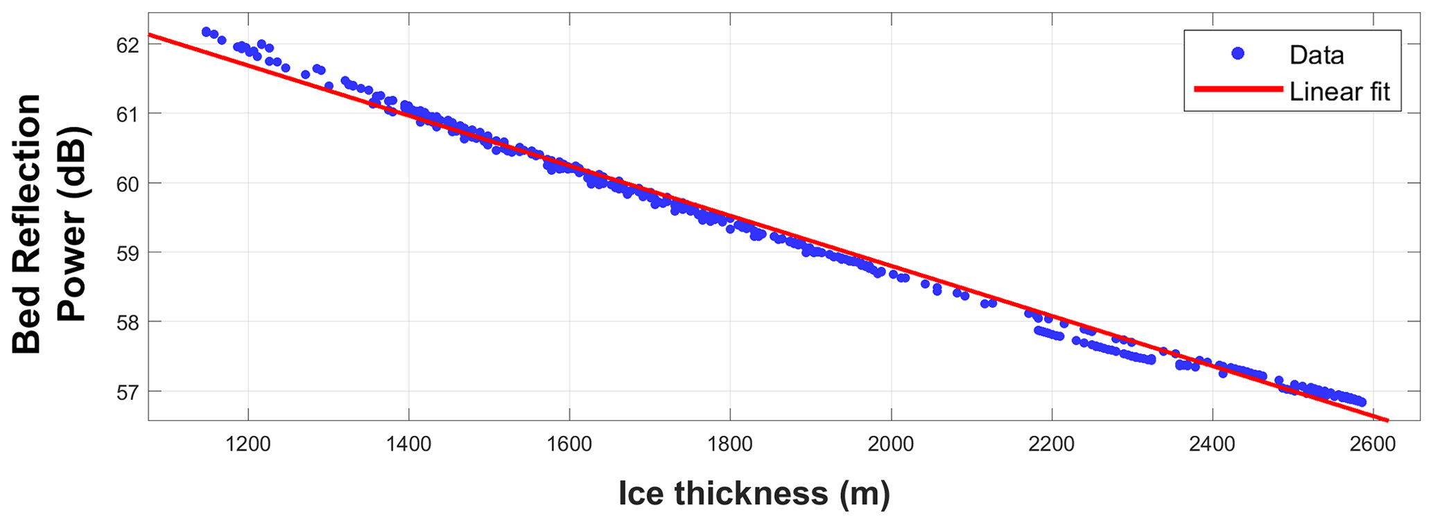
For each section of the radar profile with a subglacial-lake candidate, we quantify the ice attenuation loss (L_i) following previous studies (e.g. Winebrenner et al., 2003; MacGregor et al., 2007; Matsuoka et al., 2012; Schroeder et al., 2016) on a “section-by-section” basis. We first use an empirical relationship between the ice thickness (Z_s) and BRP; and we then apply a depth-averaged attenuation rate to correct for the power loss (Fig. 2). To calculate the bed reflection power estimated (BRP_e), we substitute the L_g calculation and the L_i estimation into Eq. (3).

Figure 2 Example of the ice attenuation correction for a window of PASIN radar data (BBAS line B01; SL2 in Fig. 7). The red best-fit line is a log of normalised power representing the bed reflection power (BRP) dependency on ice thickness.

2.3 Specularity calculation

In this work we use the standard deviation (σ) of the BRP as a proxy to infer the surface specularity of each potential water body (Carter et al., 2007). This is used as a threshold to determine whether the surface of each subglacial-lake candidate is smooth or not (Peters et al., 2005). σ was calculated with 20 samples either side of a particular point, i.e. ∼ 400 m each side, to ensure a representative number of radar observations are included. A low value of σ indicates a smooth surface is present at the base of the ice as would be expected for the surface of a water body (e.g. Peters et al., 2005; Carter et al., 2007).

2.4 Subglacial-lake classifications

Having identified the candidate subglacial lakes, we determine the degree of confidence in our identification by ranking them from the most to least likely to be a subglacial lake. To achieve this we initially use the BRP values for each lake candidate following previous work (Carter et al., 2007), comparing these values to known subglacial water bodies such as SLE, SLC and Lake Vostok. This leads to a suite of four physically based categories to which each potential subglacial lake is assigned, ranging from definite to indistinct as follows:

1. Definite subglacial lakes. This category has an absolute reflectivity higher than the surroundings (BRP at least 15 dB higher) and displays low variation in BRP (high specularity, < 3 dBσ BRP). Therefore, this category is defined by a high absolute reflection power and a low standard deviation (σ) across the candidate subglacial-lake surface.

2. Dim subglacial lakes. These candidates have a high relative reflection strength and surface specularity but lack the absolute reflectivity values of definite lakes in that their BRP is no more than 10 dB higher than the surroundings.

3. Fuzzy subglacial lakes. These candidates show higher relative and absolute reflection coefficients than the surroundings but are not specular along their surfaces (i.e. > 3σ BRP). We note that a challenge with such candidates is that they could also potentially be saturated basal sediments (Dowdeswell and Siegert, 2003; Peters et al., 2005; Siegert, 2000). In addition, if the water is less than 8 m deep, reflections from the water–lake bottom interface may interfere with the signal from the ice–water interface (Gorman and Siegert, 1999). Furthermore, exceptionally smooth surfaces with no water present could also have similar signal characteristics to these fuzzy subglacial lakes (Carter et al., 2007).

4. Indistinct subglacial lakes. This category is composed of lake candidates that are specular but have a reflectivity that is difficult to distinguish from the surroundings. Although these could still represent subglacial lakes, such characteristics are also common to transient water systems or to exceptionally smooth beds with fine-grained sediments surrounded by rougher saturated sediments (Carter et al., 2007).

2.5 Hydropotential (Φ) calculation

To determine the subglacial hydrological characteristics of the EWM region, we produced a new bed digital elevation model (DEM). We use existing gridded bed elevation data from Bedmap2 (Fretwell et al., 2013), ice thickness from DELORES (2007–2009) and CECs (2005/06; Siegert et al., 2012), along-track ice thickness measurements from the 2014 CECs RES campaign (Rivera et al., 2015), and new unpublished radar measurements from the CECs 2017 RES field campaign in the ESH region (Zamora et al., 2019; Uribe et al., 2019). In January 2014 ∼ 1100 km of RES data collected by CECs over an area of ∼ 7000 km² were acquired with a line spacing of ∼ 8 km. The CECs survey during December of the same year was collected over a nested grid around SLC and along the host subglacial trough further north towards RIS, surveying a total of ∼ 1050 km. During December 2017 the CECs radar survey acquired a total of ∼ 700 km of RES data along the same trough (Fig. 3).

Figure 3 Coverage of data sets used in the construction of the bed digital elevation model. Blue lines show data from Bedmap2 and SLE DELORES surveys; black lines show catchment boundaries produced using data from the SCAR Antarctic Digital Database v7.1 (https://www.add.scar.org/, last access: 21 September 2020). Red lines show new radar lines from CECs surveys. Projection: Antarctic Polar Stereographic (EPSG:3031).

We used a 2 km grid mesh with a continuous curvature tension spline algorithm (Paxman et al., 2017; Wessel et al., 2013) to grid the data. We masked the grid to remove interpolated values more than 5 km from the nearest measured data point and replaced them with Bedmap2 bed elevation values. As Bedmap2 has a resolution of 1 km, we used the nearest-neighbour algorithm to downsample the DEM cell size to 2 km. We also masked the ice shelves from the radar measurements and replaced these values with those from Bedmap2 to obtain offshore bathymetry. The 1 km resolution CryoSat-2 ice surface DEM (Slater et al., 2018) was downsampled to 2 km to match the new bed DEM using the nearest-neighbour routine. This enabled us to use the ice surface elevation and subglacial bed to determine the hydrological head, Φ, following Shreve (1972).

At the ice sheet bed, water flows in the direction of the steepest descent of the hydraulic potential. Hydropotential (Φ_h) is the sum of the water pressure, P_w (Pa), and water density, ρ_w (1000 and 1020 kg m⁻³ for fresh water and seawater, respectively), normalised by the gravitational acceleration, g (9.8 m s⁻²), and the water system bed elevation, Z (m; e.g. Shreve, 1972; Cuffey and Paterson, 2010; Livingstone et al., 2013), as follows:

$$\begin{array}{}\text{(5)}& \mathrm{\Phi }=P_{\mathrm{w}}+{\mathit{\rho }}_{\mathrm{w}}gZ.\end{array}$$

Equation (5) can be rewritten into an alternative equation in terms of subglacial bed and ice surface elevation (Shreve, 1972).

$$\begin{array}{}\text{(6)}& \mathrm{\Phi }={\mathit{\rho }}_{\mathrm{w}}gZ+k{\mathit{\rho }}_{\mathrm{i}}gH,\end{array}$$

where ρ_i is the density of ice (917 kg m⁻³); H is the ice thickness (m); and k is a dimensionless factor, representing the influence of ice overburden pressure on the local subglacial water pressure.

We assumed the water pressure is close to the ice overburden pressure as suggested for the ESH in previous studies (e.g. Vaughan et al., 2007; Rivera et al., 2015), so Eq. (6) can be rearranged as follows:

$$\begin{array}{}\text{(7)}& \mathrm{\Phi }={\mathit{\rho }}_{\mathrm{w}}gZ+{\mathit{\rho }}_{\mathrm{i}}gH.\end{array}$$

This approach has been widely used across Antarctica to model the subglacial hydrological drainage (e.g. Livingstone et al., 2013; Carter et al., 2017; Kirkham et al., 2019).

2.6 Subglacial-water flow routing

Because subglacial water moves from areas of high to low subglacial water pressure, following the hydropotential gradient (Shreve, 1972), we can determine present-day large-scale subglacial flow routing and identify whether the candidate subglacial lakes connect into this subglacial hydrological network. We modelled the subglacial flow routing using the hydropotential and followed Schwanghart and Scherler (2014) to calculate the flow routing using the following steps:

1. Lows (sinks) in hydropotential were filled to their lowest pour point.

2. The channelised network was then determined using a multiple-flow-direction (MFD) algorithm (Schwanghart and Scherler, 2014). The subglacial hydraulic drainage basin was then delineated, and we computed the flow accumulation in order to understand the upstream contributing area above the lakes.

3. The stream network was then defined using an upslope area threshold for channel initiation. We set an arbitrary threshold of 25 connected cells (50 km²) as defining a channel.

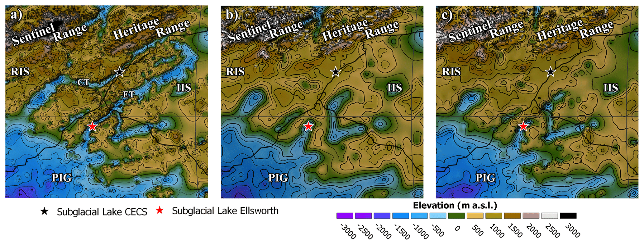
Figure 4 Comparison between three different bed digital elevation models. (a) New DEM gridded in this work; (b) Bedmap2 DEM; (c) BedMachine Antarctica v1. White lines show the catchment boundaries produced using data from the SCAR Antarctic Digital Database (https://www.add.scar.org/, last access: 21 September 2020). ET: Ellsworth Trough; CT: CECs Trough; RIS: Rutford Ice Stream; PIG: Pine Island Glacier; IIS: Institute Ice Stream. Projection: Antarctic Polar Stereographic (EPSG:3031).

3 Results

3.1 New bed elevation model

The new bed DEM of the ESH provides new detail on two major subglacial troughs – Ellsworth Trough (ET) and a parallel trough east of ET, informally referred to here as CECs Trough (CT; Fig. 4) – and shows that they are much deeper than shown in existing DEMs (e.g. Bedmap2 and BedMachine Antarctica v1). These troughs extend parallel to the Ellsworth Mountains and are extensive linear features that appear to connect the interior of the ESH to the deep basins that lie beneath the WAIS. These are a common feature within the ESH and likely reflect a topography which has evolved under conditions of alpine glacial erosion, fluvial erosion and tectonic processes prior to glacial inception (Jamieson et al., 2014; Sugden et al., 2017; Vaughan et al., 2007; Ross et al., 2014). This area may have been subject to a mix of areal scour and selective linear erosion beneath the WAIS (e.g. Jamieson et al., 2014; Sugden et al., 2017; Paxman et al., 2019). The main difference from Bedmap2 and BedMachine Antarctica v1 are (1) the two parallel subglacial troughs that run from IIS to RIS and PIG and (2) a subglacial mountain range between the new troughs with a perpendicular transection valley near SLE (Fig. 4). In Fig. 4, we compare these new features in our DEM against Bedmap2 and BedMachine Antarctica v1.

3.2 Subglacial lakes

Using qualitative visual analysis of the BBAS radar data, we identified 107 bright reflections potentially caused by subglacial lakes within the BBAS data set (Fig. 5). These reflections were further analysed by comparing the characteristics of these features with other Antarctic subglacial lakes (Siegert, 2005; Carter et al., 2007) in order to either confirm or reject each feature as a subglacial lake (Fig. 6).

The lakes are largely distributed within a series of subglacial valleys that emerge from the ESH into the Bentley Subglacial Trench near the ice divide between PIG, RIS and IIS at the northern edge of the ESH (Fig. 7). We observe two clusters of subglacial lakes and one potential chain of subglacial lakes in the ESH region. The first cluster is near SLE, < 100 km from the ice divide between IIS, RIS and PIG (Fig. 8a). Most of the subglacial lakes in this first cluster are located in ET or are connected to the same trough system. However, in some cases the drainage of subglacial water in this cluster may be in two distinct directions, i.e. towards the Weddell Sea Embayment (WSE) or ASE (Fig. 8c). The second cluster is located in a valley in the upper PIG catchment near the water divide between the ASE and the WSE (Fig. 8b). Hydraulic modelling suggests that this cluster drains towards the WSE (Fig. 8d). Furthermore, the subglacial hydrological simulation also shows that part of the drainage flowing beneath PIG is diverted to flow beneath Thwaites Glacier (TG), collecting the water of these ice catchments and draining to the ASE.

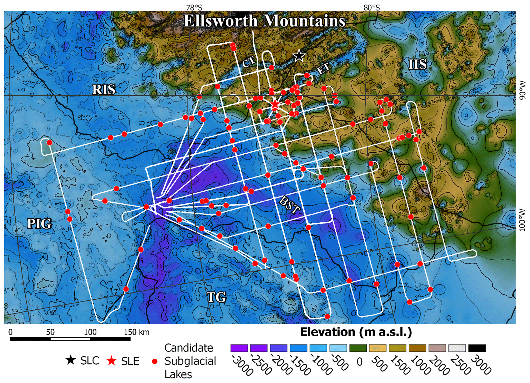
Figure 5 Qualitative analysis of high-amplitude reflection (red dots) identified using eight flight lines of the BBAS radar set. The black and red stars show the position of Subglacial Lake CECs (SLC) and Subglacial Lake Ellsworth (SLE), respectively. The red star also marks the location of the radar section shown in Fig. 6. Data from the BedMachine Antarctica v1 elevation model (500 m; Morlighem et al., 2019) are shown in the background. White lines show the 7500 km of analysed BBAS radar lines. Black lines show the catchment boundaries produced using data from the SCAR Antarctic Digital Database (https://www.add.scar.org/, last access: 21 September 2020). ET: Ellsworth Trough; CT: CECs Trough; RIS: Rutford Ice Stream; PIG: Pine Island Glacier; TG: Thwaites Glacier; BST: Bentley Subglacial Trench; IIS: Institute Ice Stream. Projection: Antarctic Polar Stereographic (EPSG:3031).

Using the quantitative analysis of the bed reflectivity at 107 locations and classifying accordingly, we confirm the presence of 33 previously unrecognised subglacial lakes (information in the Supplement, Table S1), which is a ∼ 40 % increase in the total number of subglacial lakes known to exist beneath the WAIS (Wright and Siegert, 2012). Although a small number of these subglacial lakes were hypothesised or identified by other studies (e.g. Livingstone et al., 2013; Vaughan et al., 2007), none of these water bodies were included in the most recent subglacial-lake inventory of Wright and Siegert (2012). Using the categories described above, we categorise these subglacial lakes into four groups with different confidence levels (Fig. 7). We identify 7 definite subglacial lakes (very high confidence), 5 dim subglacial lakes (high confidence), 20 fuzzy subglacial lakes (medium confidence) and 1 indistinct subglacial lake (low confidence).

3.3 Distribution of subglacial lakes

The ESH host 24 of the new subglacial lakes; 7 others are in the Bentley Subglacial Trench, and 2 lakes are located in the region of relatively high topography between tributaries 3 and 5 of PIG, between Byrd Subglacial Basin and the outlet of PIG (SL21 and SL22 in Fig. 7). A majority of these subglacial lakes (30) are located less than 50 km from the ice divide, and 13 are located within 20 km of the ice divide between IIS and RIS (Fig. 9a). Sixteen small subglacial lakes (less than 3 km in length) lie within 30 km of an ice divide, and the two largest subglacial lakes (SL6 and SL23) are located within 25 km and ∼3 km of the PIG ice divide, respectively. The ice thickness over the small subglacial lakes is variable, ranging from 1600 to 4000 m with an average thickness of ∼2600 m (Fig. 9b). Five subglacial lakes are covered by ice thicker than 3000 m thick, and 10 lie underneath ice less than 2000 m thick. Most subglacial lakes associated with thinner ice columns are located south of the IIS–PIG ice divide, while those underneath thicker ice columns are distributed at the head of PIG. A majority of subglacial lakes with an overlying ice thickness of between 2000 and 3000 m are situated close to the triple ice divide between IIS–RIS and PIG and along the border between PIG and RIS, where the ice surface slope is near zero (Fig. 9d) and, hence, the subglacial hydraulic gradient is also close to zero. Those subglacial lakes located near the PIG–RIS–IIS ice divide lie beneath very slow flowing ice (Figs. 9c and 10). However, the ice surface velocity is higher (between 50 and 60 m yr⁻¹) above those subglacial lakes located at lower elevations (Fig. 10). The length of subglacial lakes is variable, ranging from a minimum of ∼0.35 km to a maximum of ∼8 km, but most (18) are less than 2 km in length (Fig. 9e). Some of the subglacial lakes (13) are larger than 2 km, and two (SL6 and SL23), near the PIG ice divide (Fig. 7), are relatively large lakes (∼8 km). In addition, the new DEM reveals that subglacial lakes are located within two different subglacial topographic contexts: within linear subglacial troughs with steep side walls and within lowland terrain constrained by subglacial hills (Fig. 4).

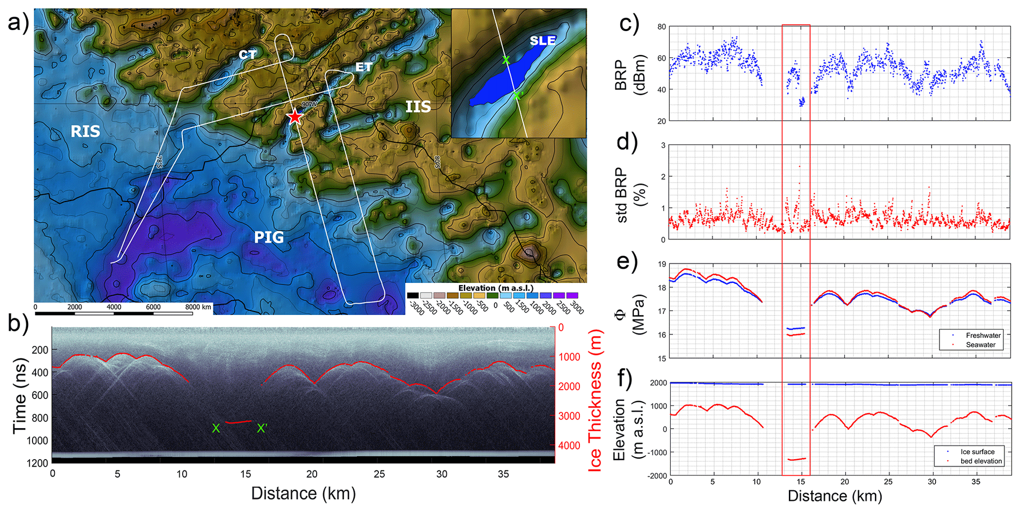
Figure 6 Example of subglacial-lake identification in a radargram from the BBAS survey (flight line B05) and its location in the WAIS. (a) The location of the flight line (B05, white line) and the position of the radargram (red star) in the line overlaid on the new subglacial DEM (2 km). Ice catchment boundaries produced using data from the SCAR Antarctic Digital Database v7.1 (https://www.add.scar.org/, last access: 21 September 2020) are shown in black. The inset on (a) shows the SLE bed topography contour, and the portion in the profile above SLE between x and x' represents the subglacial lake in (b). ET: Ellsworth Trough; CT: CECs Trough; RIS: Rutford Ice Stream; IIS: Institute Ice Stream; PIG: Pine Island Glacier. Projection: Antarctic Polar Stereographic (EPSG:3031). (b) The bright reflection (red line) classified as a subglacial lake. The radargram shows both the time (ns) for the returned echo from the ice–bed interface and the ice thickness (m) calculated using a radio wave propagation through the ice of 0.168 m ns⁻¹. (c) Bed reflection power (dBm). (d) Specularity (σBRP). (e) Hydropotential considering freshwater (blue) and saltwater (red) densities. (f) Ice surface elevation (blue line) and bed elevation (red line).

3.4 Subglacial flow routing

The modern configuration of the ice sheet and the improved bed DEM allowed us to calculate a new hydropotential map around the ESH. This hydropotential model suggests that the subglacial water catchment of the WAIS differs in shape to those previously calculated. The new hydraulic potential model suggests an increase of ∼ 1500 km² in the water catchment area of TG (in comparison with Bedmap2), mainly because of the contribution of the newly discovered CT (Fig. 4). The water flow routing in the hydrological network initiates near the major ice divides in the region (i.e. RIS–IIS–PIG) and flows to the margin of the continent (Fig. 7d and e). The hydraulic model assumes a wet bed throughout the ESH, and the geometry of the subglacial hydrological network is classically dendritic. It extends almost from the major ice divide (RIS–IIS–PIG) to the edge of the ice sheet, connecting the majority (i.e. 30 subglacial lakes) of the subglacial lakes identified in this work into a wider subglacial hydrological network. We identify two main drainage systems: the WSE and ASE. There are 15 subglacial lakes draining towards the WSE and 18 draining towards the ASE. In the ASE, most of the subglacial lakes are connected into a single drainage network flowing underneath PIG and TG and partially beneath RIS. Only two subglacial lakes are disconnected from the main ASE drainage system: they originate near the border between RIS and PIG over the subglacial highland (SL28) and within a valley subparallel to ET (SL31). Only one subglacial lake, located in the upper catchment of IIS (SL10), is disconnected from the WSE drainage system. Significantly, we note that the surface flow patterns of ice and the flow patterns of subglacial water are not always coincident. The most evident difference between hydrological and ice flow catchments is observed underneath the PIG–TG catchments (Fig. 8c and d). Here, the ice flows from the PIG–IIS ice divide into the PIG catchment; however the subglacial drainage catchment flows first into the head of the PIG catchment and then diverts into the TG catchment. We find that the area of the subglacial hydrological catchments of PIG and TG are ∼ 1.35×10⁵ and ∼ 2.83×10⁵ km², respectively (if calculated using BedMachine Antarctica v1, they are ∼ 1.25×10⁵ and ∼ 2.88×10⁵ km², respectively). These are markedly different to the ice surface catchments of PIG and TG, which have areas of ∼ 1.76×10⁵ and ∼ 1.86×10⁵ km², respectively (Mouginot et al., 2017).

Figure 7 Location of subglacial lakes within the Ellsworth Subglacial Highlands. Inset: location of the ESH in Antarctica. The subglacial lakes are represented by different shapes and colours according to the classification of their BRP. The subglacial lakes are classified from a greater to a lesser degree of confidence as follows: red dots for definite, yellow squares for dim, pink diamonds for fuzzy, and cyan diamonds for indistinct subglacial lakes. The black and red stars represent SLC and SLE, respectively. In the background the new subglacial DEM and the PIG tributaries are numbered according to the scheme given by Stenoien and Bentley (2000). Contours are every 500 m. The red rectangle shows the location of (a) and (b) (also c and d) in Fig. 8. Catchment boundaries produced using data from the SCAR Antarctic Digital Database v7.1 (https://www.add.scar.org/, last access: 21 September 2020) are shown in thick black lines. ASE: Amundsen Sea Embayment; BST: Bentley Subglacial Trench; BSB: Byrd Subglacial Basin. Projection: Antarctic Polar Stereographic (EPSG:3031).

We find that a majority of the known subglacial lakes in the region coincide with channels delineated in our subglacial hydraulic modelling. This gives additional confidence to the assessment of the lakes because it provides an indication not only that there are upstream areas which might capture enough water to fill a lake but also that the routing would be appropriately directed to deliver that water into the lake locations. A challenge with the subglacial flow routing is that the bed DEM is based on sparse data due to the reconnaissance nature of the primary airborne RES data sets across the study area. As a consequence, the interpolation across gaps in the DEM means that the routing is subject to uncertainty associated with overly smooth data in some areas and potentially noisy data in others. Because we use tension spline interpolation, we believe that noise is minimised.

4 Discussion

4.1 Subglacial lakes and the production of basal water

We have identified several bright basal reflections, which we interpret as subglacial lakes. Many of these are located at the head of the catchments of PIG and TG, and many are very close to the ice divide between IIS, PIG and RIS (Fig. 7). Because some of these were classified as “definite” lakes, we have confidence that they may be up to as much as 100 m deep like SLC and SLE. The subglacial water may be produced by a combination of basal melting directly over subglacial lakes and the input of water produced elsewhere in the subglacial catchment (e.g. Ross and Siegert, 2020).

The spatial distribution of subglacial lakes in terms of size does not have an evident pattern. The RES data show that most of the subglacial lakes (∼ 60 %) are smaller than 2 km and only ∼ 10 % are bigger than 5 km. Only ∼ 30 % of the subglacial lakes are between 2 and 5 km in length and are distributed within a region of steep subglacial topographic relief (e.g. the ESH), while the smaller subglacial lakes are found in much lower subglacial terrain. However, the largest new subglacial lakes are also located in a low-elevation area, underneath RIS. The distance from the lakes previously inventoried to the ice divide is similar to our new lakes, confirming the tendency of subglacial lakes to be located close to the thick, flat ice and rough basal topography associated with ice divides (Dowdeswell and Siegert, 1999). While Wright and Siegert (2011) mapped subglacial lakes as large as ∼ 10 km, the subglacial lakes identified in this work are all less than 8 km in length. Despite this, the predominance of lakes with lengths less than 3 km is similar to the distribution noted by Wright and Siegert (2011).

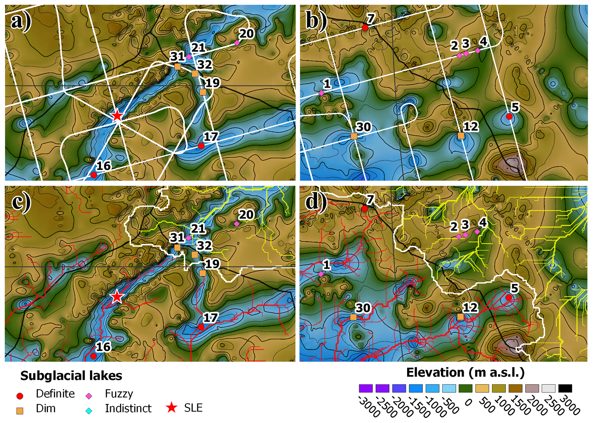
Figure 8 Two main subglacial lakes clusters: Ellsworth Trough and the western ESH. The location of this cluster is delimited by red squares in Fig. 7. (a) First cluster of subglacial lakes in Ellsworth Trough. (b) Second cluster of subglacial lakes identified in the upstream Institute area. The new subglacial DEM is shown in the background. In (a) and (b) white lines are airborne RES survey tracks. Elevation contour lines are at 500 m intervals. (c, d) The subglacial water hydrological network, for the same areas of (a) and (b), plotted in different colours depending on the flow direction. The red lines show modelled subglacial drainage towards Amundsen Sea Embayment (ASE); the yellow lines show drainage to the Weddell Sea Embayment (WSE). In (c) and (d) the white lines show the subglacial water catchment boundaries, and the thick black lines show the ice sheet boundaries produced using data from the SCAR Antarctic Digital Database (https://www.add.scar.org/, last access: 21 September 2020.). Projection: Antarctic Polar Stereographic (EPSG:3031).

Subglacial lakes are likely to form beneath areas suitable for the existence of basal meltwater, for example in areas of thick ice (i.e. > 2.5 km) where the pressure melting temperature is enough to maintain liquid water (Dowdeswell and Siegert, 1999; Gorman and Siegert, 1999), in areas of internal ice deformation and sliding that contribute heat to produce melting (Siegert et al., 1996), or in areas of elevated geothermal heat flux (GHF). Observations of GHF are absent in the ESH, and modelled GHF estimates (e.g. Shapiro and Ritzwoller, 2004; Maule et al., 2005; An et al., 2015; Martos et al., 2017) vary depending on the technique used and may not show localised highs in the GHF. This allows for the possibility of localised elevated GHF and therefore enhanced production of basal water in the ESH. One potential localised source of elevated basal heat is enhanced radiogenic heat flux from granite intrusions known to exist within the EWM block (Burton-Johnson et al., 2017; Leat et al., 2018). In addition, the high-relief basal morphology of the ESH (e.g. Vaughan et al., 2007; Ross et al., 2014; Winter et al., 2015), with their narrow and deep subglacial troughs, will enable a localised intensification of GHF via topographic focusing (van der Veen et al., 2007). Continent-wide models of the basal thermal regime (e.g. Pattyn, 2010) suggest that the ESH are warm-based throughout, although given the thin ice located between the deep subglacial troughs, it is more likely to have a patchwork basal thermal regime, with warm-based ice within the deep troughs and cold-based ice on the subglacial interfluves. Beyond the ESH (e.g. PIG, RIS, TG) it is likely that the bed is predominantly warm-based in line with continent-scale models (e.g. Pattyn, 2010). The discrepancy between the Pattyn model and actual basal conditions in the ESH is likely to be due to the coarse resolution of Bedmap data (Lythe and Vaughan, 2001) used by Pattyn (2010). Future numerical modelling of the basal thermal regime using our new high-resolution DEM and newly identified subglacial lakes would therefore be an important aspect of improving assessments of the basal thermal regime in this region.

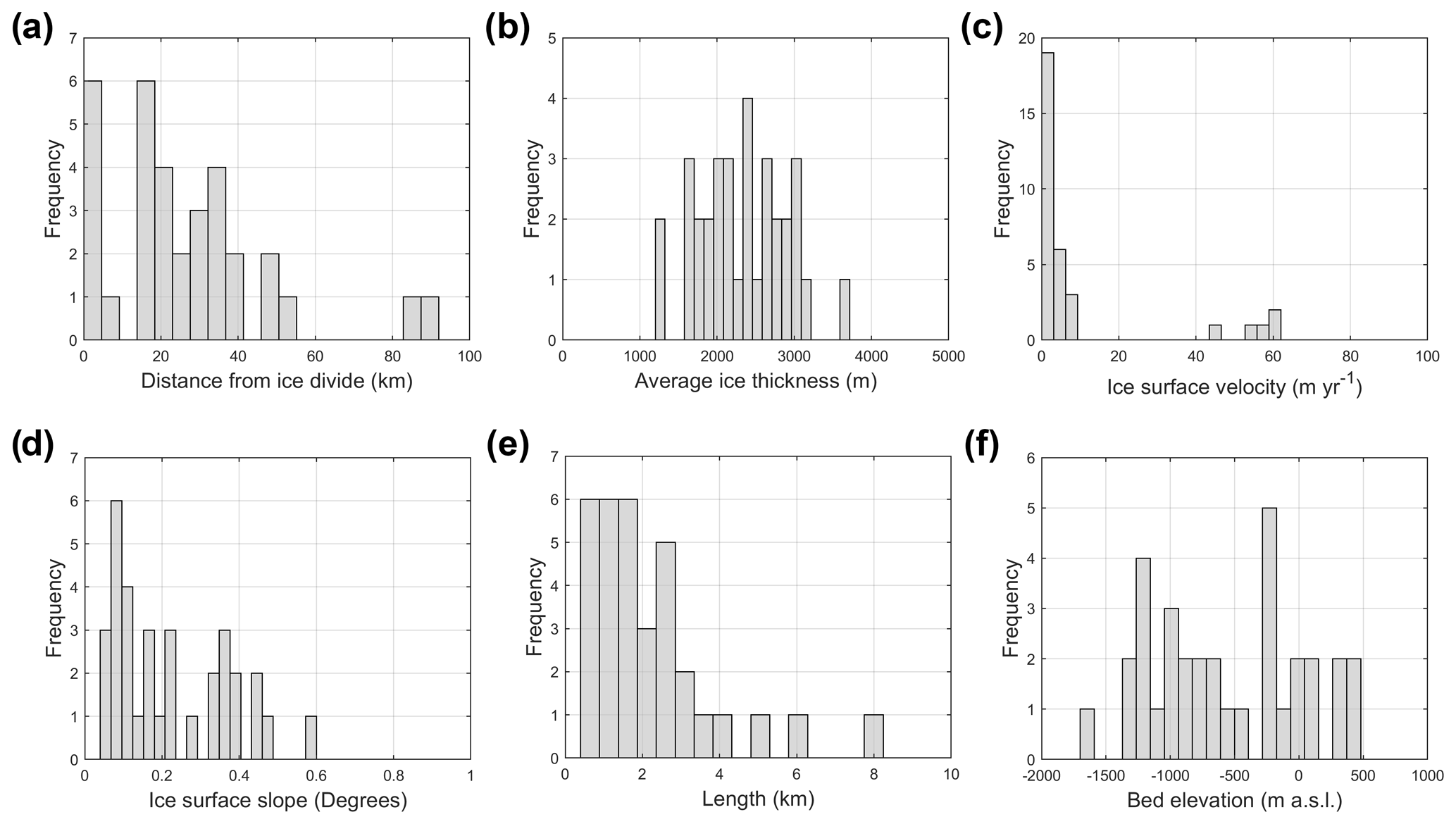
Figure 9 Frequency–distribution histograms of subglacial lakes identified in this study. (a) Distance from major ice divides. (b) Average ice thickness, obtained from BBAS ice thickness measurements. (c) Ice surface velocity (Mouginot et al., 2019). (d) Ice surface slope, obtained using CryoSat-2 (Slater et al., 2018). (e) Minimum length of identified subglacial lake, calculated by measuring the horizontal extent of the lake reflection. (f) Subglacial-lake bed elevation (new DEM).

4.2 Large-scale subglacial drainage network and lake connectivity

In the ESH, the subglacial water network is mainly controlled by subglacial topography and pre-existing troughs and deep valleys (e.g. ET and CT; Siegert et al., 2012). Flow routing into the Bentley Subglacial Trench, RIS, IIS and TG is determined by the combination of the steep-sided trough walls and the overall form of the ice sheet surface, which partially aligns with ice flow. The new hydropotential map suggests that the subglacial water in the ESH is flowing along the axis of the new deep subglacial troughs (i.e. CT and ET) and is likely connected with the northern edge of the ESH. This implies that more water than previously expected is draining through the TG subglacial water catchment, potentially lubricating its bed.

It is possible that the subglacial lakes identified in the Ellsworth Trough (Fig. 8c) are connected in a very well defined local drainage system (Siegert et al., 2012; Ross and Siegert, 2020). The hydropotential modelling also shows that the subglacial hydrological divide between water flowing into the WSE and ASE is less than ∼ 20 km upstream of SLE and most of the seven subglacial lakes in this system are connected or very close to a subglacial water path. This raises the possibility that some episodic events could link these subglacial lakes by draining subglacial water from one hydropotential sink to another, from areas with high hydraulic potential (i.e. modern ice divide between PIG and IIS) to areas with lower hydraulic potential (i.e. the Bentley Subglacial Trench), forming a cascade-type system (e.g. Smith et al., 2017). However, these bridging events may not be large enough to displace the necessary subglacial water along this flow path for detection by remote sensing methods. Another possibility is that these episodes occur on the timescale of tens of years, and therefore they may not be noticed from the surface. We also identify a dim subglacial lake (SL16) in CT, downstream of SLC towards RIS (Fig. 7). Although the current hydraulic modelling does not show a clear connection between this new lake and SLC, it is possible that under different ice sheet configurations both subglacial lakes were connected hydrologically. Alternatively, this lack of connection could be related to uncertainty in topography or because the model we used to simulate the drainage system does not accurately represent the current hydrological regime.

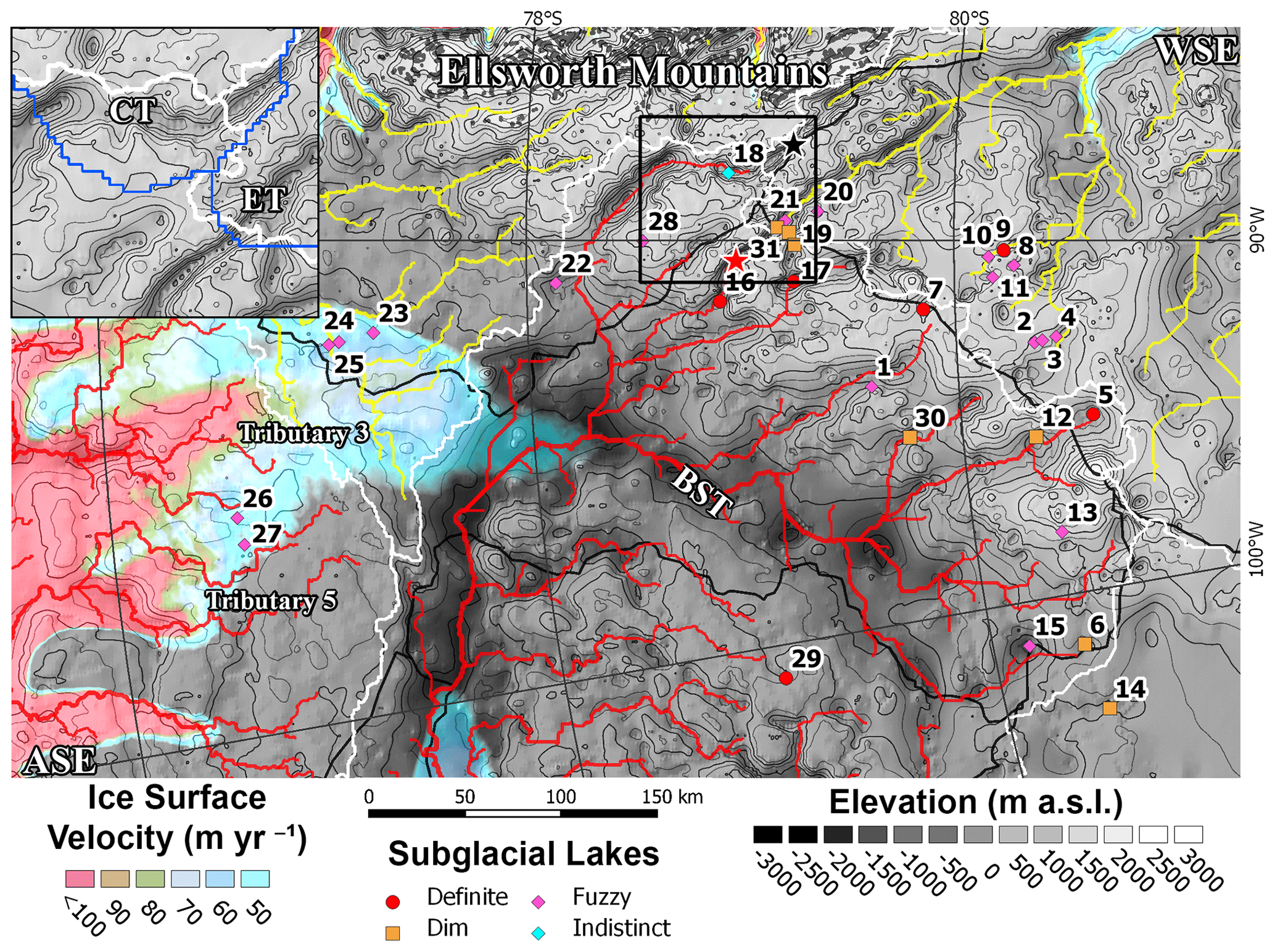
Figure 10 Mean annual ice surface velocity (Mouginot et al., 2019) of Pine Island Glacier, the Rutford Ice Stream, the Institute Ice Stream and Thwaites Glacier. The red lines show the subglacial water towards the Amundsen Sea Embayment (ASE), while the yellow lines indicate the drainage towards the Weddell Sea Embayment (WSE). The inset in the upper corner (black square in main panel) shows details in the water catchment boundary between the ASE and the WSE. ET: Ellsworth Trough; CT: CECs Trough. The white line indicates the boundary of the water catchment (this work), and the blue line indicates the previous boundary (Bedmap2). Ice surface velocity (Mouginot et al., 2019) and the new DEM are shown in the background, with elevation contours every 500 m (thin black lines). Velocities lower than 50 m yr⁻¹ are not displayed. BST: Bentley Subglacial Trench. Projection: Antarctic Polar Stereographic (EPSG:3031).

4.3 The subglacial hydrological catchments of Pine Island and Thwaites glaciers

We observe that most of the subglacial water draining towards the ASE is routed through the Bentley Subglacial Trench in the upper part of the hydrological catchment and driven through the Byrd Subglacial Basin towards the trunk of TG. The high topography in the centre of PIG catchment (Vaughan et al., 2006) means that the hydrological drainage system does not link to the faster-flowing trunk of PIG (Fig. 10) and instead the basal hydrological system is captured by TG. This drainage pattern has two main implications. Firstly, the subglacial hydrological catchments of PIG and TG do not correspond to the ice catchments; they do not coincide in either position or size. Secondly, the hydrological system of the TG trunk (Schroeder et al., 2013) may be fed by water sourced in the upper glaciological catchment of PIG, within the ESH.

Following from this, any change in the water catchment of TG, at the head of PIG, could therefore have important glaciological consequences for the ice dynamics of TG and the wider ASE. This is particularly critical because the subglacial water drainage area of TG is larger than previously thought and recent investigations (e.g. Smith et al., 2017) have demonstrated the presence of active subglacial lakes, in a cascade-type system, beneath the trunk of TG. Any water accumulation or drainage (e.g. chain of active subglacial lakes) in this area may therefore affect the basal friction of the ice and therefore the ice flow velocity. Conversely, this pattern may have a reduced importance for PIG in terms of magnitude or timing due to the topographic barrier disconnecting the drainage upstream with the lower or marginal section of PIG. If we are to clearly understand the potential role of subglacial water on the ice dynamics of the PIG and TG systems, then more detailed investigations of the subglacial and hydrological conditions are required.

4.4 The spatial relationship between subglacial lakes and ice flow in West Antarctica

Almost 90 % of the newly identified subglacial lakes in West Antarctica are located in areas of slow ice flow velocity (< 20 m yr⁻¹; Mouginot et al., 2019). There are two likely reasons for this: firstly, the ice surface slope, which is a crucial driver of basal hydraulic conditions, is typically low in these regions (Supplement, Table S1), thus enabling ponding to occur even in relatively low-magnitude topographic depressions. Secondly, given the ice flow is slow in this area, we can infer that the subglacial network may be an efficiently draining system that does not enable the pressurisation of a deforming bed but instead may allow efficient water transport.

4.5 Limitations of the RES data, the bed DEM and hydropotential modelling

The BBAS radar data were processed as unfocused SAR images and were based on 1-D reflection (Heliere et al., 2007). In some areas (e.g. subglacial troughs), this provided a poor constraint on the subglacial bed because of the presence of diffracted hyperbolae caused by an unfocused return of the energy. This means the ice–bed interface is not clear enough to identify in some of the radar lines, and it is especially difficult to detect the bed topography in areas where the strength of the radar return is low. This way of processing could have influenced the BRP calculation, causing some subglacial-lake classification to be misleading or underestimating the size of the recognised subglacial lakes due to an uncertainty as to which axis (longitudinal or transversal) had been identified.

The BRP calculation was focused in single portions with bright reflectors on each radar profile; and we assume a constant ice attenuation rate by considering the attenuation within these portions as proportional to the ice thickness. Although this attenuation is proportional to the dielectric attenuation, and therefore to the ice temperature and to solute content in the ice (Gudmandsen, 1971; Corr et al., 1993), we did not include any temperature model, which resulted in a limited capacity to distinguish differences in reflectance.

We categorised every subglacial lake based on its physical characteristics using the classification method proposed by Carter et al. (2007) as a guideline. However, specularity criteria could be modified by increasing the threshold to 6 dB σ as suggested in previous studies (e.g. Gudmandsen, 1971; Peters et al., 2005), allowing some roughness in the ice–bed interface, and considering the values for the same criteria in SLE and SLC. In this case, the number of definite subglacial lakes would rise to 17, while the number of fuzzy lakes would decrease to 10 subglacial lakes (Supplement, Table S2).

Our new subglacial DEM improves our previous knowledge of subglacial bed conditions in the ESH (Bedmap2, Fretwell et al., 2013, and BedMachine Antarctica v1, Morlighem et al., 2019). Despite its relatively coarse resolution, it does account for topographic features which connect the WSE with the ASE that are not yet present in the Bedmap2 and BedMachine Antarctica v1 DEMs (Fig. 4). We note that our hydropotential model was derived from this new gridded DEM at a resolution of 2 km, and therefore it may not detect some smaller (< 2 km) subglacial flow pathways. Although new and/or more detailed subglacial water or drainage systems could be identified in future RES campaigns, the main hydrological outlets would not be substantially different to those which we have identified under the modern ice sheet configuration.

Additional targeted surveys across the newly identified lake reflections would better constrain the size and area of the subglacial lakes and therefore improve our estimations of the potential volume of subglacial lakes within this region of the WAIS. Moreover, for the parts of the survey closest to the ESH, the BBAS survey collected airborne RES using a regular 30 km grid flown at constant altitude (Vaughan et al., 2006), which could have missed some features and/or subglacial lakes hosted in areas between each flight line. Therefore, the number of subglacial lakes discovered in this work could increase with more RES data acquired using a grid optimised to characterise the subglacial interface, considering the geometry of the subglacial topography. Ideally, this grid would have survey lines aligned perpendicularly to topographical features (e.g. across subglacial troughs) as opposed to diagonally.

5 Conclusions

1. We used RES data from the 2004/05 BBAS survey to locate subglacial lakes within the ESH region of West Antarctica. This analysis allowed us to identify 33 new subglacial lakes to add to the existing inventory (Wright and Siegert, 2012). We then classified these subglacial lakes according to how confident we are in their detection. Using this classification, we identify 7 subglacial lakes with a very high degree of confidence. A further 5 dim subglacial lakes, 20 fuzzy lakes and 1 indistinct subglacial lake were also identified.

2. We observed that a majority (28) of the subglacial lakes are situated underneath or close to (< 40 km) the modern ice divide between the Institute Ice Stream and the Rutford Ice Stream, Pine Island Glacier and Thwaites Glacier. Furthermore, we also detected that slow ice flow is associated with these lakes and that there are always low-gradient ice surfaces above them.

3. We developed a new bed DEM based on recently collected radar survey data that were not previously incorporated into Antarctic topographic models. This allowed us to recognise new topographic features such as the long and linear subglacial trough systems (i.e. CT and ET) which connect to multiple sub-catchments and which therefore may play an important role in the basal hydrology and dynamics of the West Antarctic Ice Sheet.

4. Using the new DEM and the up-to-date surface elevation model from CryoSat-2 (Slater et al., 2018), we analysed the subglacial hydraulic network. We identified the potential for connection between the subglacial lakes and the wider subglacial hydrological system, thus providing a mechanism for cascading and active lake drainage. Most importantly, however, we show that the hydrological catchments of RIS, PIG and TG do not correspond precisely with glaciological catchments. Indeed, TG's hydrological catchment appears larger than previously thought, capturing basal water from the upper region of PIG.