the Creative Commons Attribution 4.0 License.
the Creative Commons Attribution 4.0 License.
 | 04 Dec 2020
The Antarctic sea ice cover from ICESat-2 and CryoSat-2: freeboard, snow depth, and ice thickness
We offer a view of the Antarctic sea ice cover from lidar (ICESat-2) and radar (CryoSat-2) altimetry, with retrievals of freeboard, snow depth, and ice thickness that span an 8-month winter between 1 April and 16 November 2019. Snow depths are from freeboard differences. The multiyear ice observed in the West Weddell sector is the thickest, with a mean sector thickness > 2 m. The thinnest ice is found near polynyas (Ross Sea and Ronne Ice Shelf) where new ice areas are exported seaward and entrained in the surrounding ice cover. For all months, the results suggest that ∼ 65 %–70 % of the total freeboard is comprised of snow. The remarkable mechanical convergence in coastal Amundsen Sea, associated with onshore winds, was captured by ICESat-2 and CryoSat-2. We observe a corresponding correlated increase in freeboards, snow depth, and ice thickness. While the spatial patterns in the freeboard, snow depth, and thickness composites are as expected, the observed seasonality in these variables is rather weak. This most likely results from competing processes (snowfall, snow redistribution, snow and ice formation, ice deformation, and basal growth and melt) that contribute to uncorrelated changes in the total and radar freeboards. Evidence points to biases in CryoSat-2 estimates of ice freeboard of at least a few centimeters from high salinity snow (> 10) in the basal layer resulting in lower or higher snow depth and ice thickness retrievals, although the extent of these areas cannot be established in the current data set. Adjusting CryoSat-2 freeboards by 3–6 cm gives a circumpolar ice volume of 17 900–15 600 km3 in October, for an average thickness of ∼ 1.29–1.13 m. Validation of Antarctic sea ice parameters remains a challenge, as there are no seasonally and regionally diverse data sets that could be used to assess these large-scale satellite retrievals.
- Article
(7475 KB) - Full-text XML
- BibTeX
- EndNote


The author's copyright for this publication is transferred to California Institute of Technology.
The gradual increase in Antarctic sea ice extent in satellite records over the last 4 decades reversed in 2014, with subsequent rates of decrease in 2014–2019 exceeding the decay rates in the Arctic. For these past years, the Antarctic sea ice extents were reduced to their lowest levels in the 40-year satellite record (Parkinson, 2019). Our current understanding of the behavior of the Antarctic ice cover is largely informed by these ice coverage measurements from satellite passive microwave sensors. Ice extent, however, provides an incomplete picture of sea ice response to climate change and variability. But, even with the large observed changes, available measurements are still too few to be able to determine the long-term trend of ice production and volume of the of Antarctic sea ice cover (Vaughan et al., 2013)
Prior to the 2014 decline in Antarctic ice extent, coupled ice–ocean models have suggested that significant changes in ice volume and thickness are correlated to changes in ice extents (Massonnet et al., 2013; Holland et al., 2014), and increases in ice thickness may have been driven by the intensification of the wind field (Zhang, 2014) noted by Holland and Kwok (2012). In addition, fully coupled climate models generally fail to capture the observed trends and variability in ice coverage during the last few decades (e.g., Mahlstein et al., 2013; Polvani and Smith, 2013; Turner et al., 2015; Zunz et al., 2013; Hobbs et al., 2015). However, large-scale estimates of ice thickness and ice production necessary to improve attribution of change, model evaluation, and improvements for projection of future behavior have been challenging to obtain. Retrievals of Antarctic ice thickness remain a research topic, largely due to uncertainties in snow depth and freeboard (Giles et al., 2008) required for computing snow loading in the conversion of freeboard to thickness.
Wide discrepancies between ice thickness estimates from recent approaches to determine sea ice thickness persist (Kurtz and Markus, 2012; Xie et al., 2013; Yi et al., 2011). Current algorithms to derive ice thickness from data collected by ICESat (Ice, Cloud, and land Elevation Satellite) have to rely on the following simplifying assumptions: (1) an independent measure of snow depth (Yi et al., 2011), (2) the snow depth being equal to the total freeboard (Kurtz and Markus, 2012), or (3) empirical relationships between total freeboard and ice thickness being determined from field data (Xie et al., 2013). All these approaches have limitations. The first approach tends to underestimate of snow depth in areas of deformed ice. The second seems more appropriate for the thinner ice in the outer pack with low ice thickness. The third method may be most suitable for thicker ice, where knowledge of densities is subsumed into the regression coefficients. Such empirical relationships vary seasonally and regionally (Ozsoy-Cicek et al., 2013), and thus the confidence in the derivations is reduced. Even so, these approaches have provided a large-scale depiction of the spatial variability of the ice and snow cover based on limited knowledge of the Antarctic ice cover.
With the launch of NASA's ICESat-2 (IS-2) in late 2018 and the extension of ESA's CryoSat-2 (CS-2) mission, we are now able to combine lidar and radar altimetry of the Arctic and Antarctic ice covers from IS-2 and CS-2 for understanding ice behavior. A recent paper by Kwok et al. (2020) demonstrated the retrieval of basin-scale estimates of both Arctic snow depth and sea ice thickness from differences in IS-2 and CS-2 freeboards. Here, we follow the same approaches to examine the large-scale seasonal cycle of Antarctic freeboards, retrieved snow depth and ice thickness from a joint analysis of IS-2 and CS-2 data (between April and November of 2019). At the outset, we note that the results from this study remain exploratory because of the current understanding of the snow cover of Antarctic sea ice. There are many aspects of data quality, some of which will only be revealed by assessment with the snow data acquired and processed by dedicated airborne campaigns (e.g., NASA's Operation IceBridge) and field programs and when a longer IS-2/CS-2 time series becomes available.
The paper is organized as follows. The next section describes the IS-2 and CS-2 freeboard data sets used in our analysis. In Sect. 3, we first discuss the key processes that contribute to the time evolution of Antarctic freeboards, and then describe the observed evolution of the two freeboards during the 8 winter months. Section 4 outlines the principle behind the derivation of snow depth from freeboard differences, the sampling of the satellite freeboards for calculation of snow depth, and the derived monthly estimates. Section 5 compares the thickness and volume of the Antarctic ice cover computed using the derived snow depth and assuming that snow depth is equal to the IS-2 freeboard. Potential biases in the data are discussed. Section 6 concludes the paper by highlighting these first observations and discuss challenges in having the appropriate data sets for assessment of the retrievals from the two altimeters.
The primary data sets are freeboards from IS-2 and CS-2. Their attributes are described below.
2.1 ICESat-2 (IS-2) freeboards
The Advanced Topographic Laser Altimeter System (ATLAS) on board ICESat-2 uses three beam pairs to profile the surface. The pairs are separated by about 3.3 km cross track. Each pair consists of a strong and a weak beam with an inter-beam spacing of 90 m. The pulse energies of the strong beams are ∼ 4 times that of the weak. Each beam profiles the surface at a pulse repetition rate of 10 kHz and footprints of ∼ 14 m (Neumann et al., 2019). Along-track freeboards are from the ICESat-2 ATL10 products (Release 002) from the National Snow and Ice Data Center (Kwok et al., 2019b). The ATL10 product provides sea ice freeboard estimates – with a variable along-track resolutions (∼ 27 to 200 m) – in 10 km segments that contain a sea surface reference. Local sea surface references (href) (i.e., the estimated local sea level) are from available sea ice leads within a 10 km segment. Freeboard heights (hf) are the differences between surface heights (hs) and the local sea surface reference (i.e., ). For individual beams, freeboard profiles are calculated with sea surface references from that beam with no dependence on estimates from other beams. In ATL10, freeboards are calculated only where the ice concentration is > 50 % and where the height samples are at least 25 km away from the coast (to avoid uncertainties in coastal tide corrections). Details of the sea ice algorithms can be found in Kwok et al. (2019a) and an early assessment of surface heights can be found in Kwok et al. (2019c). Only the freeboards from the strong beams are used in the following analyses, and cloud-contaminated retrievals are also not used. We note that, in the IS-2 data set used here, there is a 1-month gap in coverage (July) indicated in the figures due to a spacecraft anomaly and that data are only available for the first 2 weeks of November 2019 in this release of the IS-2 data set. Uncertainty in IS-2 freeboard retrievals is ∼ 2–4 cm based on assessment in Kwok et al. (2019c).
2.2 CS-2 radar freeboards
Along-track CS-2 freeboards are derived using the procedure in Kwok and Cunningham (2015), which contains a detailed description of the retrievals and an assessment of these freeboard estimates in the Arctic. The pulse-limited footprint of the CryoSat-2 synthetic aperture radar altimeter is approximately 0.31 km by 1.67 km along- and across-track. Freeboards are retrieved for individual returns but the derived CS-2 freeboards used here have been averaged to 25 km resolution and weighted by AMSR-derived ice concentration. As there are no large-scale assessments of these freeboard estimates, only comparisons with available ice thickness measurements from variety of sensors (e.g., upward-looking sonars, airborne lidars, and airborne electromagnetic profilers) provide an indirect measure of quality. Noting that freeboard is approximately one-ninth of ice thickness (due to the density contrast between, ice and seawater) differences between CS-2 and various thickness measurements in the Arctic in Kwok and Cunningham (2015) are as follows: 0.06 ± 0.29 m (ice draft from moorings), 0.07 ± 0.44 m (submarine ice draft), 0.12 ± 0.82 m (airborne electromagnetic profiles), and −0.16 ± 0.87 m (Operation IceBridge).
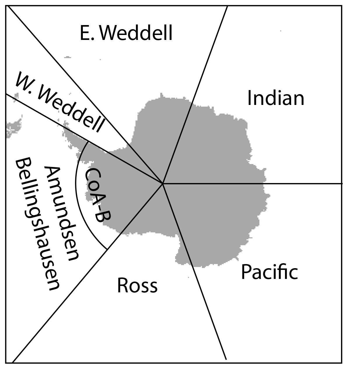
Figure 1Naming of the sea ice sectors used in the paper.
In this section, we first discuss expected time-variable changes in IS-2 and CS-2 freeboards based on our understanding of the key processes, before examining the spatial patterns and distributions of the monthly freeboards. Here, we divide the circumpolar Southern Ocean into five sectors, namely Weddell Sea, Amundsen Sea–Bellingshausen Sea, Ross Sea, Pacific Ocean, and Indian Ocean (Fig. 1); these are typically used in ice extent analyses (Comiso and Nishio, 2008). Further, we subdivide the Weddell sector into an east sector and west sector, and added a coastal Amundsen–Bellingshausen region to sample the impact of the remarkable ice convergence observed in 2019 (discussed below).
3.1 Interpretation of time-varying IS-2 and CS-2 freeboards
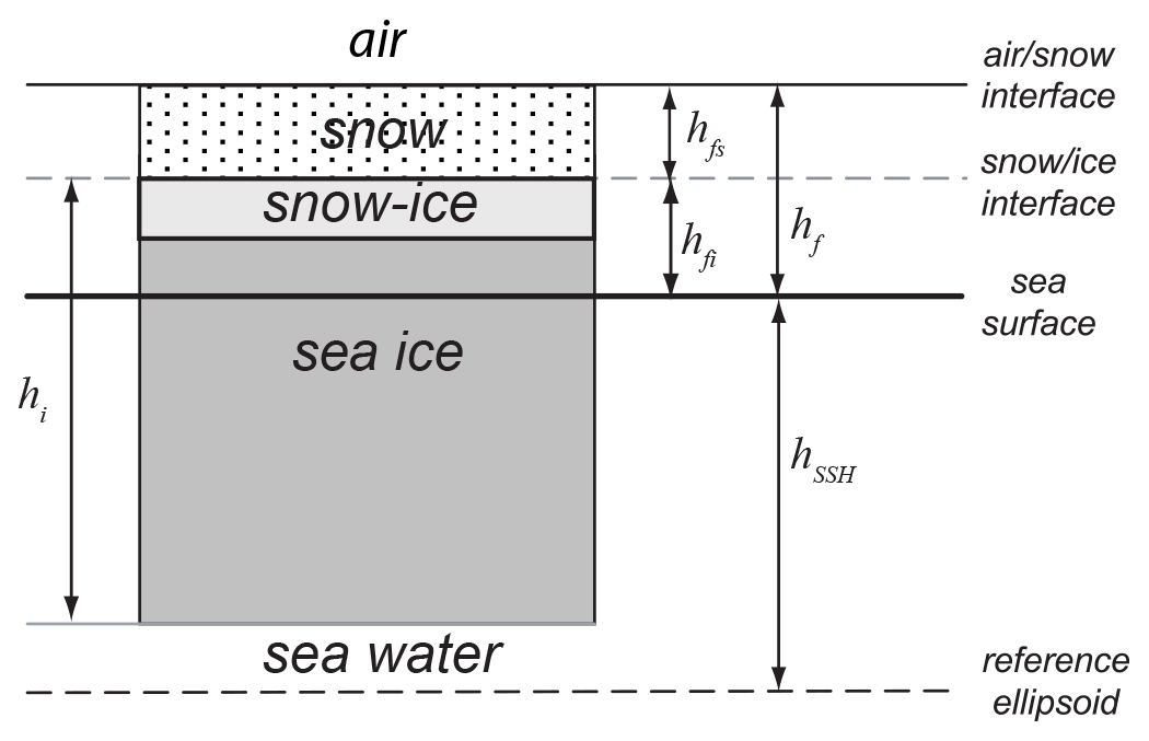
Since this is the first large-scale examination of the combined IS-2 and CS-2 freeboards of the Antarctic ice cover, it is worthwhile reviewing the key processes that contribute to regional-scale freeboard changes. This will aid in the interpretation of the observations. As a reminder, the changes in total freeboard (Δhf) are the sum of the changes in thickness of the snow layer (Δhfs) and changes in ice freeboard (Δhi), i.e., (Fig. 2). In the winter Arctic, there are three key processes that contribute to the changes in total freeboard: basal growth, ice deformation, and snow accumulation and redistribution. Since the Arctic Basin exports only ∼ 10 % of its area annually (mainly through the Fram Strait; Kwok et al., 2013), there is relatively little melt in winter away from the ice margins. Therefore, it is simpler to observe a coherent seasonal cycle of freeboard growth over a fixed region of the Arctic Basin (i.e., the correlated increases in both the IS-2 and CS-2 freeboards seen in Kwok et al., 2020). In the Antarctic, however, the heavier snowfall (Massom et al., 1997), ice production in large coastal polynyas (Drucker et al., 2011), formation of snow ice (Jeffries et al., 2001; Maksym and Markus, 2008), larger ice divergence (i.e., production of areas of open water) than the Arctic, wind-blown redistribution of the snow cover including losses into leads (Andreas and Claffey, 1995; Massom et al., 1997, 1998), and the continuous large-scale export of sea ice towards the ice margins (where the ice melts) (Kwok et al., 2017) add complexity to the interpretation of the seasonal evolution of freeboards.
Below, we briefly summarize five key processes that contribute to the modification of the total freeboard (hf) of a drifting ice parcel during the Antarctic winter. Separating the contributions from the snow (hfs) and ice layers (hfi), we write
α and β are scale factors, and signs indicate the addition or removal of height from these layers. The δh values are described below.
-
Snowfall (δhsnow). Precipitation minus evaporation (P-E) adds to the snow layer and the loading depresses the ice freeboard by −αδhsnow. α is a fractional value, and in this case it is dependent on the densities of ice, snow, and seawater.
-
Spatial redistribution of snow including loss into leads (δhϕ). Snow is redistributed due to wind stress and is sometimes lost into open leads (δhϕ); the ice freeboard adjusts hydrostatically by −αδhϕ.
-
Snow ice formation. When sea water infiltrates the snow layer during flooding, the refrozen ice layer becomes part of the ice freeboard and results in a loss of δhsti from the snow layer (i.e., the snow pack settles when flooded) and a gain of βδhsti by the ice freeboard. β represents the fraction of the snow thickness that is converted to ice freeboard after the transformation process.
-
Ice deformation (convergence and divergence of the ice cover). Mechanical redistribution due to convergence and divergence of the ice cover tends to increase and decrease, respectively, the area-averaged thickness of the snow layer () and ice freeboard (). The relationship between and may be more complicated and is hence written separately.
-
Basal ice growth and melt (δhgm). The growth and melt of sea ice adds and removes from the ice freeboard and increases and decreases the total freeboard, respectively.
This brief summary is a simplification, as there are higher-order processes such as changes due to snow metamorphism, but their area-averaged contributions to freeboard changes are likely to be small. Another factor (noted above) to bear in mind in the interpretation of regional variability of freeboard (below) is the advective change and sea ice melt at the margins.

Figure 3Monthly composites of IS-2 freeboard (hf), CS-2 freeboard , and derived snow depth for the period between April and November 2019 (25 km grid; in cm).
3.2 Monthly composites IS-2 and CS-2 freeboards
Figure 3 shows the monthly composites of IS-2 and CS-2 freeboards for April through November 2019. The associated freeboard distributions are shown in Fig. 4. The numerical values and sample statistics of the monthly distributions are in Table 2. We examine freeboard distributions of the seven sectors in the following order: Amundsen–Bellingshausen (A-B), coastal Amundsen–Bellingshausen (CoA-B), East Weddell and West Weddell (E-Wedd, W-Wedd), Ross, Pacific Ocean, and Indian Ocean.
3.2.1 Amundsen and Bellingshausen seas sectors (A-B and CoA-B)
The freeboard distributions of the Amundsen and Bellingshausen seas between the Antarctic Peninsula and 140∘ W are constructed with samples from two sectors (Fig. 4a and b): one lies between coastal Antarctica and 70∘ S (referred to as the CoA-B sector) and the other has an open boundary to include the seaward extent of the advancing winter ice edge (A-B sector).
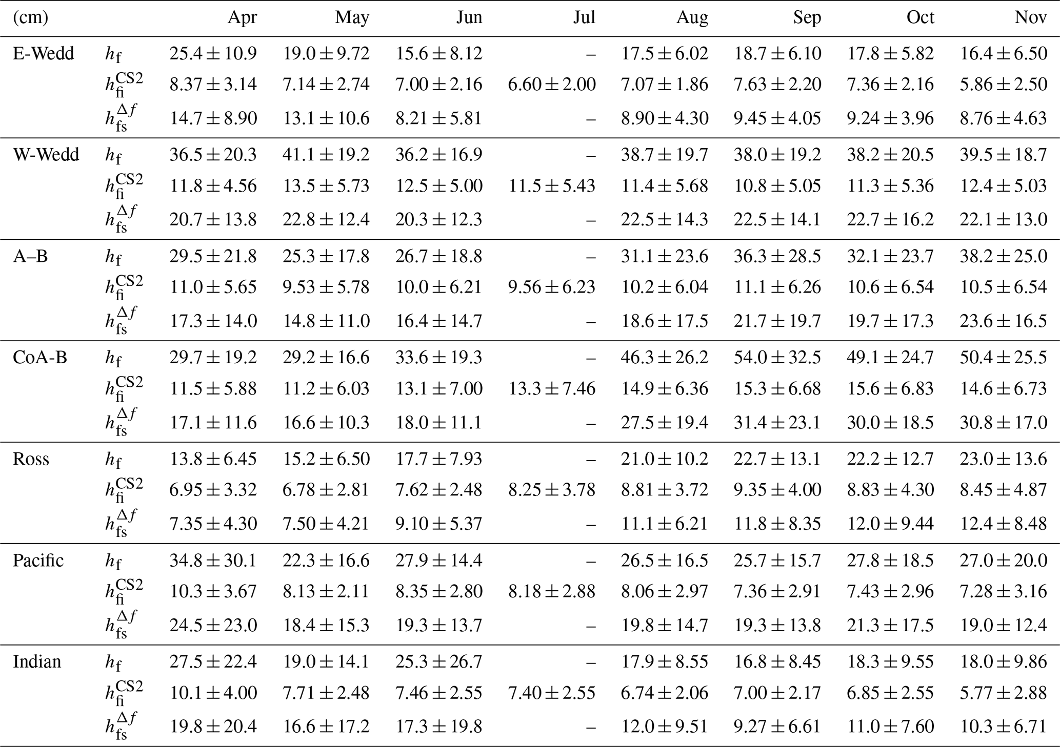
For the 8 winter months, the highest variability (amongst the seven sectors) is seen in the CoA-B sector, where the area-averaged IS-2 and CS-2 freeboards range from 29.2 ± 16.6 (min) to 54.0 ± 32.5 (max) cm and 11.2 ± 6.03 to 15.6 ± 6.83 cm, respectively. The squared correlation (ρ2) between the two freeboards of 0.90 (Fig. 4c) – the highest of all seven sectors – indicates that the co-variability may be attributable to responses to the same forcing. Indeed, examination of the monthly maps of ice drift (Fig. 5) suggests that the correlated increases in the two freeboards is likely due to the persistent wind-driven convergence of sea ice against the Antarctic coast (west of 90∘ W). The resulting ridging in the coastal Amundsen Sea ice cover resulted in a redistribution of the thinner ice into thicker categories. This simultaneously increases both the lidar and radar freeboards. The anomalous on-shore ice drift in 2019 (Fig. 5b) can be contrasted to the mean ice drift pattern for the period 2012–2019 (Fig. 5a). The large-scale atmospheric pattern in 2019 shows the location and depth of the Amundsen Sea Low (ASL) centered in the northeast Ross Sea (Fig. 5b). The atmospheric pattern in 2019 is such that on-shore wind is nearly perpendicular to the coast and the depth of the ASL can be seen in the density of the isobars. The longer tails of the freeboard distributions seen after May are also signatures of ice convergence, where snow accumulation would be unlikely to affect the tails of both distributions, i.e., ice freeboard tends to be anti-correlated to snow accumulation. Hence, the freeboard variability here seems to be dominated by wind-driven ice deformation, which masked the signal of other processes.
For the A-B sector (which includes the CoA-B sector), the seasonal signal is more muted. The IS-2 and CS-2 freeboards range from 25.3 ± 17.8 to 38.2 ± 25.0 cm and 9.53 ± 5.78 to 11.1 ± 6.26 cm and are lower because of the thinner seasonal ice cover away from the coastal zone (CoA-B). The squared correlation (ρ2) between the two freeboards of 0.43 (Fig. 4c) is also likely connected to the large signal in the CoA-B sector in the south. In November, the increase in the IS-2 freeboard not seen in the CS-2 freeboard is potentially due the limited 2-week IS-2 coverage.
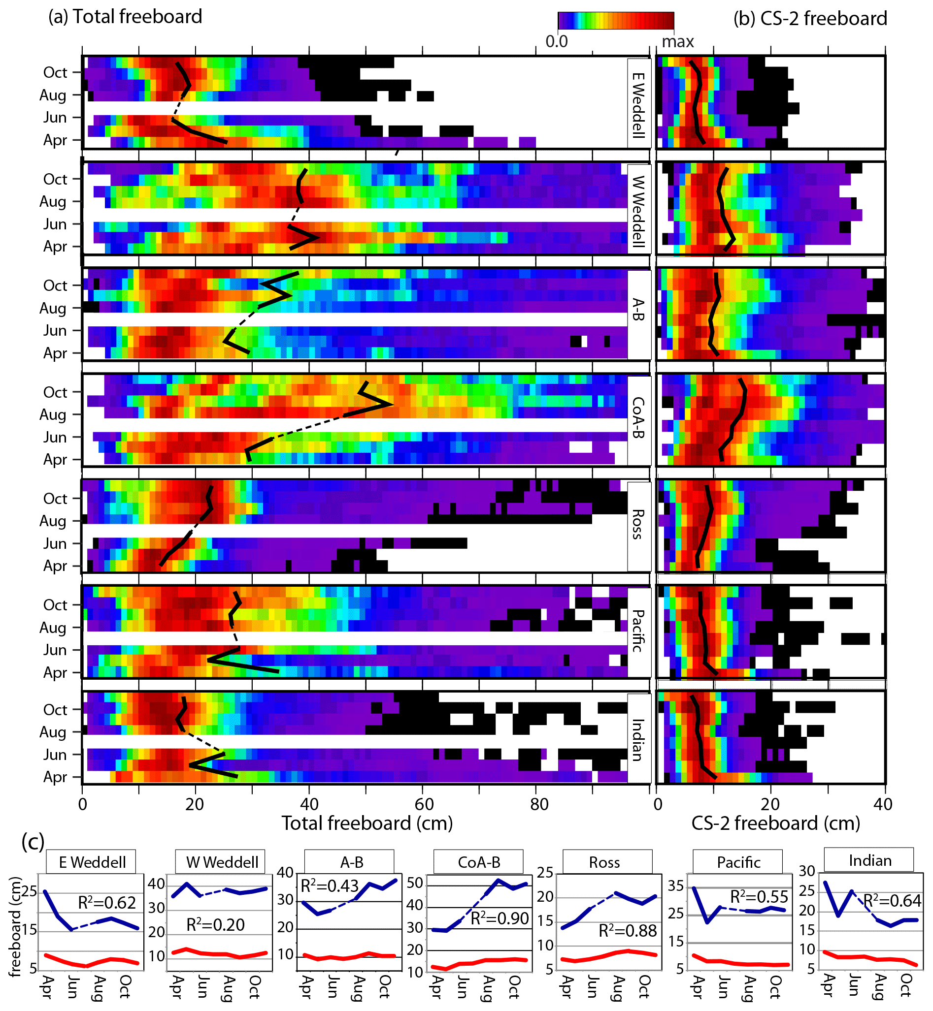
Figure 4Monthly distributions of (a) IS-2 (hf) and (b) CS-2 freeboards for the period between April and November 2019. Their monthly means are compared in (c). Numerical values in the line plots show the squared correlation between the two freeboards (distributions are normalized).
3.2.2 East Weddell Sea and West Weddell Sea sectors
The East (E-Wedd) and West Weddell (W-Wedd) sectors are located between 15∘ E and 40∘ W, and 40 and 62∘ W, respectively, both with boundaries that are open to the north. Generally, the W-Wedd sector is one of the few regions in the Antarctic where multiyear sea ice is found (Lange and Eicken, 1991). Sea ice formed in the east (E-Wedd sector) is advected clockwise around the southern Weddell Sea (cyclonic gyre), and the older sea ice is subsequently exported at its northwestern boundary after its transit (Fig. 5a). Along its drift trajectory, the ice cover becomes thicker and deformed (Lange and Eicken, 1991; Vernet et al., 2019). As well, younger and thinner ice areas added by mechanical divergence and formed seaward of the Ronne and Brunt ice shelves (Drucker et al., 2011). The average annual areal export from the southern Weddell Sea (along a flux gate along the 1000 m isobath that parallel the ice fronts of the Ronne and Filchner ice shelves) is km2 (Kwok et al., 2017) and is comparable to the area of km2 enclosed by the flux gate of ∼ 1100 km in length.
In the composite fields (Fig. 3), the thicker ice with its higher IS-2 and CS-2 freeboards in the W-Wedd sector is a feature that stands out in the circumpolar Antarctic ice cover. In the 2019 composites, an area of lower IS-2 and CS-2 freeboards (likely of ice formed in Ronne Polynya) is present in the southwestern corner of the Weddell Sea. In the 8 months of 2019 (Fig. 4c), the CS-2 freeboard only varied over a narrow range of ∼ 3 cm (i.e., between 10.8 ± 5.05 and 13.5 ± 5.73 cm). The squared correlation (ρ2) between the two freeboards is 0.20 (Fig. 4c). Unlike the clear convergence signal in the A-B sectors (correlated freeboard time series), this behavior suggests a balance of the different or competing processes discussed earlier (Sect. 3.1). Generally, the processes that would increase the IS-2 freeboards during the winter (e.g., precipitation, convergence, and growth) must have been overwhelmed by processes that would tend to lower the IS-2 freeboards (e.g., snow ice formation, loss of snow into leads, divergence, and ice export). Similarly, contributions to increases in CS-2 freeboards (due to convergence, growth, or snow ice formation) are likely balanced by precipitation and divergence, even though the CS-2 freeboards tend to be less sensitive to these changes. The longer tails of monthly freeboard distributions in the W-Wedd (Fig. 4a and b) also suggest active ice deformation. These processes cannot be resolved at the regional scale that the data is being examined at in this paper.
In the E-Wedd, the higher total and CS-2 freeboards is likely due to the thicker ice present early in April and May that become a much smaller fraction of the area of growing ice cover as the sea ice edge advances seaward. As ice coverage grows (Fig. 3), the thinner seasonal ice dominates the total area lowering the mean freeboards in the subsequent months. Both the total and CS-2 freeboards remained within a narrow range after May, again suggesting a balance of different processes that reduced their range of variability. The lowest area-averaged freeboards are found in this sector.
3.2.3 Ross Sea sector
Significant ice production occurs in this sector (between 140∘ W and 160∘ E). New ice production in the Ross Sea is located primarily in the Ross Shelf Polynya and the Terra Nova Bay (TNB) and McMurdo Sound polynyas. Annual ice production here (south of the 1000 m isobaths) is higher than that in the Weddell Sea (Drucker et al., 2011). The average annual ice area export in a 34-year record is 0.75×10⁶ km2 (at a flux gate along the 1000 m isobaths that parallels the ice front of the Ross Sea Ice Shelf). The ∼ 1400 km flux gate encloses an area of km2 to the south. On average, the southern Ross Sea exports more than its area of sea ice that is largely produced in the polynyas.
In all months of 2019, the signature of thinner sea ice with lower freeboards exported from the polynyas can be seen as a distinct tongue that extends seaward then westward beyond the Ross embayment in both the IS-2 and CS-2 freeboards composites (Fig. 3). The spatial features are consistent with the cyclonic (clockwise) drift pattern, centered over the northeastern Ross Sea associated with the ASL, in all months between June and September (Fig. 5b). The drift pattern shows a coastal inflow of thicker sea ice into the Ross Sea from the Amundsen Sea in the east that is distinctly thicker than the outflow of thinner ice from the southern Ross Sea. North of Cape Adare in the northwestern corner of the Ross Sea, the northward drift splits into two branches, with one that moves westward into the Somov Sea and another that moves northeastward before it gets entrained in the Antarctic Circumpolar Current (ACC).
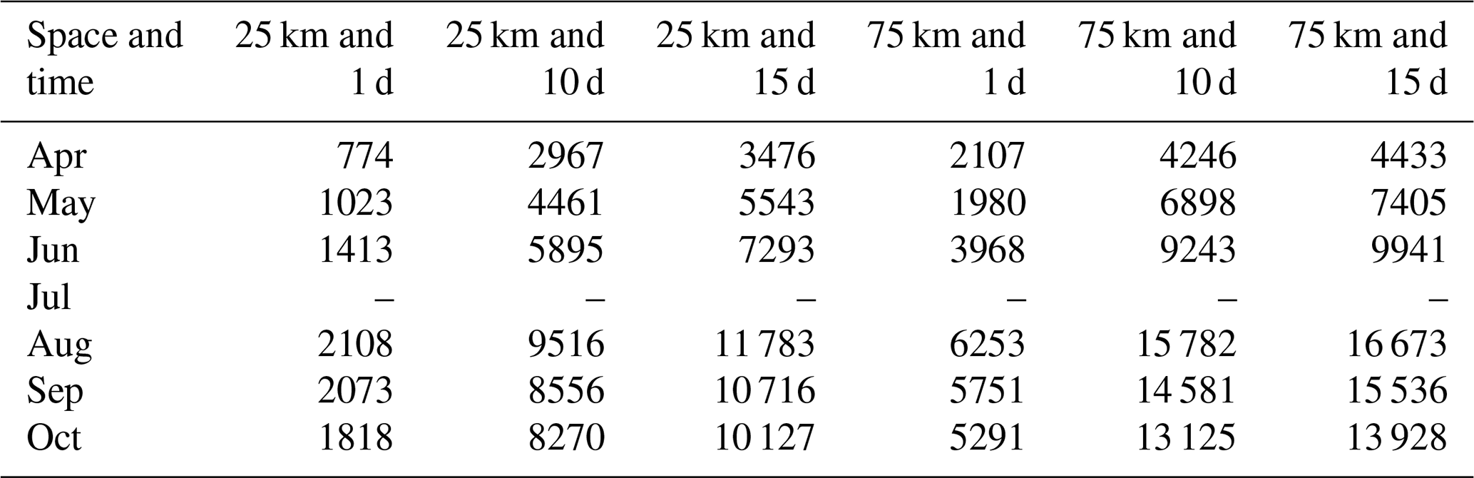
Table 1Dependence of number of retrievals on space–time separation. November is not included here because the IS-2 data (Release 002) covered only half the month.
The IS-2 and CS-2 freeboards range from 13.8 ± 6.45 to 23.0 ± 13.6 cm and 6.78 ± 2.81 to 9.35 ± 4.00 cm, respectively (Fig. 4c, Table 1). Both freeboards show a gradual increase, with a peak in the IS-2 freeboard during August, likely due to overlapping coverage of the ice convergence events by the A-B (discussed above) and Ross sectors and due to inflow of the thicker deformed ice from the A-B sector. The squared correlation (ρ2) between the two freeboards of 0.88 (Fig. 4c), comparable to that in the CoA-B sector, is likely due to the continual production of thin ice in the polynyas, the growth of the thin ice as it is advected northward, and the northward drift and growth of the sea ice from the A-B sector.
3.2.4 Pacific Ocean and Indian Ocean sectors
The Pacific Ocean and Indian Ocean sectors are located between 90∘ E and 160∘ W and 15 and 90∘ E, respectively. Except for the larger extent of the ice cover in the Indian Ocean sector (around 15 and 40∘ E), where the winter edge extends into the South Atlantic and Indian Oceans, the ice cover occupies a very narrow band that extends only ∼ 400 km seaward at its maximum extent. In 2019, associated with the location of the Davis Strait Low (DSL) pressure pattern (Kwok et al., 2017), there is an average westward ice drift in both sectors in all months that is consistent with that seen in the mean 2012–2019 drift patterns (Fig. 5a). The Pacific Ocean sector ice cover is composed of mainly seasonal ice formed locally and fed by coastal polynyas and outflows from the Ross Sea. Similarly, the Indian Ocean sector is largely seasonal ice grown locally and in coastal polynyas and coming from the Pacific Ocean sector.
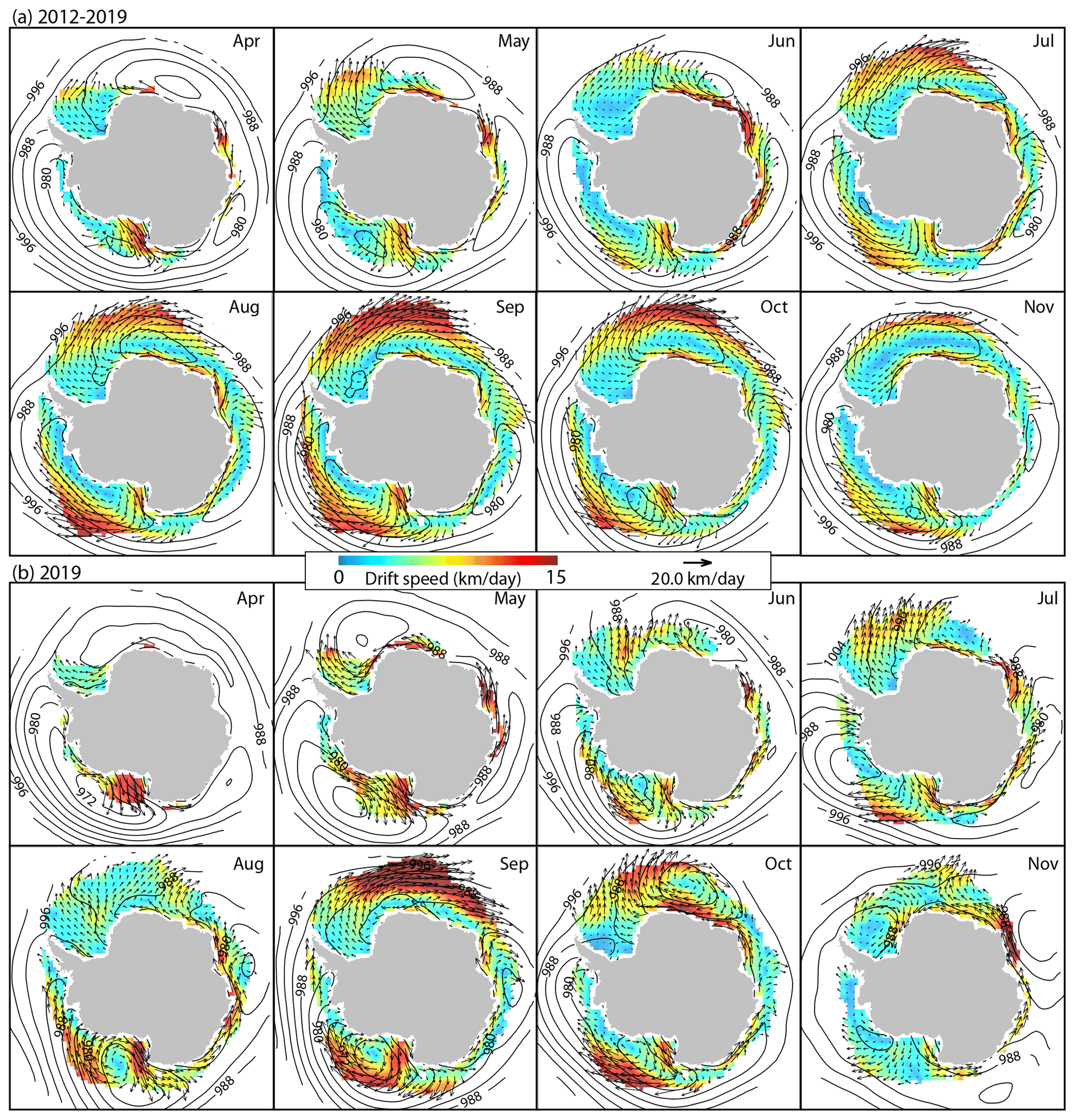
Figure 5Monthly mean (April through November) ice drift in the Southern Ocean for (a) 2012–2019 and (b) 2019.
The behavior of the freeboards in both sectors is similar (except for in magnitude) (Fig. 4). The higher IS-2 and CS-2 freeboards (though less pronounced in the CS-2 freeboards) in April–May are from a small population of sea ice adjacent to the coast (see Fig. 3). Broadly, we find it difficult to explain the source of higher freeboard sea ice in both sectors early in the growth season. The behavior of higher freeboards of both the IS-2 and CS-2 freeboards are consistent – the squared correlations (ρ2) between them are 0.55 and 0.64 in the Pacific Ocean and Indian Ocean sectors, respectively. From a retrieval perspective, we also note that the heights of the local sea surface estimates near the ice edge are affected by sea state, likely due to scattering from the troughs of waves propagating into the ice cover. This effect is predominant in the Pacific and Indian Ocean sectors because of the smaller sea ice extent. The consequence is surface heights that may be tens of centimeters below the local mean sea level, resulting in higher freeboards. We have filtered most of these anomalous freeboards (visually) in the IS-2 and CS-2 processing, but some are still present.
In general, the behavior of the sea ice cover in the Pacific Ocean and Indian Ocean sectors resembles that of the E-Wedd sector, with the lowest end-of-season IS-2 and CS-2 freeboards. The thinner seasonal ice dominates the behavior of the mean freeboards in all months (Fig. 3). The lowest CS-2 freeboards are found in the Indian Ocean sector in November (5.77 ± 2.88 cm). The CS-2 freeboards remained within a narrow range after May, the lowering of the IS-2 freeboards over the winter months suggests a balance of the different processes discussed above. Again, it is difficult to resolve these processes at the regional scale that the data is being examined at in this paper.
In this section, we first briefly summarize the calculation of snow depth from freeboard differences and the sensitivity of the retrieved snow depths to uncertainties in bulk density. Second, we discuss the procedure used to construct monthly composites with freeboards from the two altimeters and the expected uncertainties from the lack of coincidence between the two measurements. Third, the 2019 spatial patterns of snow depths are examined. Finally, we discuss the large-scale relationship between snow depth and IS-2 freeboard in the monthly composites.
4.1 Snow depth from freeboard differences
We follow the procedure detailed in Kwok et al. (2020) (henceforth K20) using a layered geometry depicted in Fig. 2. A layer of snow ice, an important component of the Southern Ocean ice cover, is included and assumed to have the same bulk density as sea ice. In our simplification, the snow ice layer is considered to be part of ice layer (hi) and indistinguishable from sea ice insofar as mechanical loading or hydrostatic equilibrium is concerned; this is necessitated by our lack of knowledge on how to effectively model the snow ice formation process. The snow depth (hfs) can thus be expressed as the difference between the total freeboard (hf) from IS-2 estimates and sea ice freeboard (hfi):
The snow depth is then given by
assuming that the scattering from the snow ice interface dominates the returns at Ku-band wavelengths (CS-2 altimeter). With one free parameter, ηs, this equation relates snow depth to the IS-2 and CS-2 freeboard differences (i.e., the two observables here): ηs is the refractive index at Ku-band, (Ulaby et al., 1986); c is the speed of light in free space; and ρs is the bulk snow density. Equation (3) accounts for the reduced propagation speed of the radar wave (cs) in a snow layer with bulk density ρs. At temperatures below freezing, the lidar and radar returns can be assumed to be from the air–snow and snow–ice interfaces, respectively, and thus they provide observations of total and ice freeboards. The validity and shortcomings of this assumption and its implications are discussed in Sect. 6. A bulk snow density of 320 kg m−3 is used in all our calculations. There is no generally accepted value for the bulk density of snow in the Antarctic. Massom et al. (2001) suggest 200–300 kg m−3 under cold and dry conditions and higher density (320–500 kg m−3) for warm and windy conditions, which is not unlike the Arctic. Below, we elected to use an average winter bulk density of 320 kg m−3 (like that of the Arctic) but with a higher variability of 70 kg m−3 to cover the range of conditions.
4.1.1 Sensitivity of snow depth and ice thickness to snow density
Similarly, following K20, we write the sensitivity of to bulk density (for the parameterization of ηs given above) as
which gives the fractional change in snow depth associated with a change in density as
Relative to a nominal density of 320 kg m−3 and an uncertainty in density of ±70 kg m−3, the uncertainty in the snow depth is ∼ 4 % of the difference in freeboard. In effect, this represents ∼ 1 cm uncertainty in snow depth for freeboard differences of 30 cm, suggesting that snow depth is relatively insensitive to uncertainties in the bulk density. The sign indicates that snow depth will be underestimated if the density is overestimated.
In addition, the sensitivity of thickness estimates to uncertainties in snow density in K20 (for a fixed total freeboard) is written as
The fractional change in ice thickness associated with a change in density is
Again, relative to a nominal density of 320 ± 70 kg m−3, the calculated thickness uncertainty is ∼ 70 % of the difference in freeboards. For a 30 cm freeboard difference (typical winter value used as an example), this translates into ∼ 0.2 m uncertainty in thickness. If the density is overestimated, the snow depth is underestimated (see above) and the ice thickness is overestimated; a larger fraction of the total freeboard is now assigned to the higher density sea ice. The above values serve as bounds on the expected density-induced errors in the retrieval estimates if a Δρs of ±70 kg m−3 is indeed representative of the density variability of Antarctic snow cover. In our simple model to convert freeboard differences to snow depth, the above analysis quantifies the expected sensitivity of the calculations to snow density.
4.1.2 Sensitivity of freeboard sampling for snow depth calculations
The sampling of the IS-2 and CS-2 freeboards for snow depth calculations follows the procedure in K20. Since Antarctic sea ice is found at lower latitudes, coverage is challenging due to the lower density of ground tracks from polar orbiting satellites. First, daily along-track IS-2 and CS-2 freeboards are averaged separately onto their own 25 km grid. Gridded IS-2 freeboards are averages of the three strong IS-2 beams and thus provide a better sampling of the spatial mean (compared to single-track profiles of CS-2 freeboards). Freeboard differences are then computed at each IS-2 grid cell using CS-2 freeboards (weighted by ice concentration) with time separations d and within a 75 km box. We find that this sampling strategy provides the best spatial coverage without sacrificing precision.
We examined the sensitivity to space–time sampling (as in K20), by assessing differences in calculated snow depths with time separations of d, < 10 and < 15 d, using CS-2 freeboards at colocated grid cells only and then freeboards within a 75 km box (i.e., including the eight neighboring grid cells); this provides six space–time combinations. The standard deviations of the differences in calculated snow depths (for the six combinations) were all less than 1 cm. This suggests that the spatial variability of the CS-2 freeboards is lower than IS-2 freeboards. As seen in the Sect. 3.2, the range of the area-averaged IS-2 freeboard between April and November (13.8 to 54.0 cm) is more than triple the range of the CS-2 freeboards (5.77 to 15.6 cm). The added advantage of longer time separations and looking over longer distances for CS-2 freeboards is the improved coverage for constructing full composites. In fact, a time-separation of 10 d (i.e., d) provides the best coverage (see Table 1).
4.1.3 Ice deformation
The episodic and localized nature of ice deformation and the impact of this process on differencing freeboards separated in time are discussed in K20. Here, we provide a brief summary. The time order of freeboard sampling has an asymmetric effect; i.e., the impact of a convergence or divergence event separating the freeboard samples would be different. If the selected CS-2 freeboard precedes an IS-2 freeboard in time, the snow depth would be overestimated (underestimated) if a convergence (divergence) event occurred in the interim. If the selected CS-2 freeboard is from a later time and a convergence (divergence) event occurred in between, the snow depths would be underestimated (overestimated). Also note is that the loss of snow during a convergence event may have a confounding effect. Here, the selected CS-2 freeboards are centered on the time of the IS-2 samples; hence, random events around that center time would increase the snow depth variance but would have a small impact on the average monthly snow depth. These results, discussed in the previous section, suggest that the effect of sea ice deformation in biasing the snow depth estimates may be small. For the six combinations of space–time sampling of the two freeboards, the variability in retrieved snow depths was less than a centimeter.
Table 2Monthly mean (standard deviation) of IS-2 freeboard (hf), CS-2 freeboard , and derived snow depth .
4.2 Snow depth estimates in 2019
The monthly snow depth composites and their distributions are shown in Figs. 3 and 6a, respectively. Table 2 shows the numerical values. Due to the low variability of the CS-2 freeboards, the spatial pattern of the snow depth estimates and the IS-2 freeboards are highly correlated in all the sectors (ρ>0.95 – see Fig. 7). Here, we summarize the spatial features of note. A more in-depth discussion of the relationship between snow depth and freeboard can be found in the next section, and an assessment of the quality of the snow depth estimates (whether they are biased) is given in the following section and Sect. 5, where these estimates were used to calculate ice thickness.
The thickest snow is seen in the W-Wedd sector (sector mean of 22.8 ± 12.4 cm in May) and the CoA-B sectors (31.4 ± 23.1 cm in September). With the multiyear sea ice cover in the W-Wedd sector, thicker snow is expected. The thinnest snow is found in the Ross (7.35 ± 4.30 cm in April) and E-Wedd (8.21 ± 5.81 cm in June) sectors. The thinner snow depth in the Ross sector is likely due to the extensive coverage by thin and young ice exported from the active Ross Sea polynyas, and in the E-Wedd sector this is likely due to the large seasonal ice cover. Lower snowfall rates may also contribute to these results (Cullather et al., 1998; Toyota et al., 2016). The spatial patterns show consistent thinning of the snow cover towards the ice margins almost everywhere and in all months; we see no spatial anomalies in snow depth near the ice edge that are expected of higher precipitation. Except for coastal zones with active polynyas (e.g., southern Ross and Weddell seas), snow depth is generally higher in coastal zones.

Figure 6Monthly distributions of (a) derived snow depth and (b) ice thickness (hi) for the period between April and November 2019 (distributions are normalized).
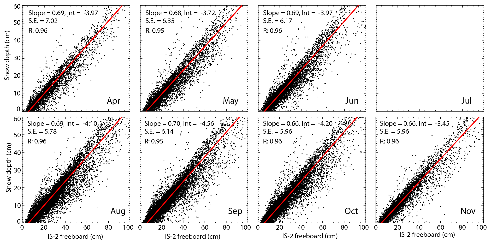
Figure 7Monthly relationship between snow depth and freeboard. Parameters from the regression analysis (slope, intercept, correlation coefficient, and standard error) are shown in the top-left corner of each panel.
Seasonal increases in the monthly mean snow depth are seen only in the A-B and CoA-B sectors. In the CoA-B sector, the increase is ∼ 13 cm (approximately half that of the IS-2 freeboard increase) over the 8 months. This is likely due to precipitation delivered by the on-shore wind pattern linked to the location and depth of the Amundsen Sea Low (ASL) discussed earlier. In all other sectors, we find slowly varying snow covers between April and November, similar to the observed behavior of IS-2 and CS-2 freeboards. This is quite remarkable and suggests the processes that remove snow from the surface (e.g., snow ice transformation, loss into leads, divergence) must be significant and overwhelm all precipitation signals in all months. Consequently, an in-depth study of these processes will be important for understanding of the behavior of the Antarctic snow cover.
4.3 Relationship between freeboard and snow depth
K20 examined the relationship between freeboard and retrieved snow depth for the Arctic ice cover. This is of geophysical interest as the connection could be potentially utilized to provide rough estimates of snow depths where there are gaps in CS-2 observation. Figure 7 shows the monthly scatterplots of and Antarctic IS-2 freeboard for the 8 months between April and November. At the length scale of 25 km, the regression analysis (slope, intercept, and standard error in each plot) of the monthly fields shows that the two values are highly correlated (with the freeboard explaining > 90 % of the variance in snow depth); this is not entirely surprising as snow depth is derived from IS-2 freeboard. The regression slopes vary between 0.66 and 0.70 between April and November. For this Antarctic winter at least, the results suggest that between 66 and 70 % of the IS-2 freeboard is snow. This can be contrasted with the 2019 Arctic winter (K20) where snow occupies a lower fraction or ∼ 50 %–55 % of the IS-2 freeboard.
The negative intercepts of between −3.4 and −4.5 cm are worth noting, as one should expect (by definition) zero snow depth at near-zero IS-2 freeboard. The consistent values of the monthly intercepts suggest that one of the estimates may be biased. Here, we write
where is the snow depth estimate and α and β are the regression slope and intercept. If zero snow depth is expected at zero total freeboard, then an unbiased estimate of snow depth (hfs) can be written as
where δ is the bias. To obtain the true unbiased estimate of snow depth (hfs), an adjustment of by δ (or −β) is needed. The negative intercepts observed in the scatterplots imply that is overestimated by +3.4 to +4.5 cm.
One likely source of these biases is the displacement of retracking point (RP) of the radar altimeter (CS-2) away from the snow–ice interface, resulting in higher CS-2 freeboards (Kwok, 2014). At Ku-band frequencies (CS-2), the RPs are displaced from the true ice surface when elevated snow salinities (due to brine-wicking, flooding) are found near the snow–ice interface or because of changes in scattering in the presence of moisture in the snow layer when air temperature warms (Winebrenner et al., 1994). For Antarctic sea ice in particular, the salinity of snow layer was characterized by Massom et al. (1997) to include two components: (1) a “background” salinity < 1 in the upper part of the snow column, likely contributed by blowing snow due to wicked salt, aerosol, or sea spray transported during strong winds over adjacent leads and polynyas, and (2) a high-salinity (> 10) basal component (0–3 cm), which is sometimes damp due to brine-wicking when the snow is thin or associated with flooding of the snow interface. It is the basal-layer salinity that has a large impact on CS-2 freeboards. Massom et al. (1997) also noted that basal salinities exceeding 10 commonly occur under relatively thin snow covers when brine is available at their surface for vertical uptake into an accumulating snow layer.
The displacement of the RPs above the snow-ice interface from radar penetration experiments in the field has been reported in a number of publications (Willatt et al., 2010, 2011). Using salinity profiles from snow pits (collected in the Canadian Arctic Archipelago) to drive a scattering model, Nandan et al. (2017, 2020) prescribed a nominal adjustment (δ) of ∼ 7 cm of the RP from first-year ice throughout most of the year. Kwok and Kacimi (2018), in an analysis of data from CS-2 and OIB, also reported consistently higher CS-2 radar freeboards along an airborne transect of the Weddell Sea.
K20 showed that an adjustment of the snow depth (δ), due to the displacement of the scattering surface, would decrease the ice thickness estimates by
A 7 cm adjustment results in a reduction in the estimated ice thickness of −0.37 m. The physical basis of a displacement of the RP due to brine wicking is sound, but a better understanding of the time evolution of these processes and the magnitude of this adjustment is needed if these corrections are to be applied to individual freeboard estimates. This will be addressed in more detail in the discussion of thickness calculations in the next section.
In this section, we first describe the calculation of ice thickness and volume by using snow depths from freeboard differences, and by assuming that the snow depth is equal to the total (or IS-2) freeboard. Second, we briefly discuss the spatial statistics of the composites and address the potential biases due to effects of the snow layer on CS-2 freeboard retrievals. Finally, the volume of the Antarctic ice cover is discussed.
5.1 Ice thickness and sector volume
We calculate two ice thicknesses: (1) hi, using snow depth from altimeter freeboards, and (2) , by setting snow depth equal to the total freeboard
In the first equation, we assume that the radar-derived surface is from the snow–ice interface. The ice thickness, , in the second equation sets a lower bound on the thickness estimates for a given total freeboard of hf, with assumed densities of water, snow, and ice (ρw=1024 kg m−3, ρs=320 kg m−3, ρi=917 kg m−3). When flooding and snow ice formation occur and the ice freeboard is zero, an estimate of total freeboard (i.e., snow depth) can be used to estimate ice thickness (given reasonable values for snow and ice densities).
Ice volume for each Antarctic sector is simply the product of the average thickness and area Asec of each sector,
To examine the potential impact on ice volume due to biases in CS-2 freeboards due to salinity effects, we write
where δ is the adjustment factor that accounts for the displacement of the CS-2 freeboard above the snow–ice interface discussed in Sect. 4.3.
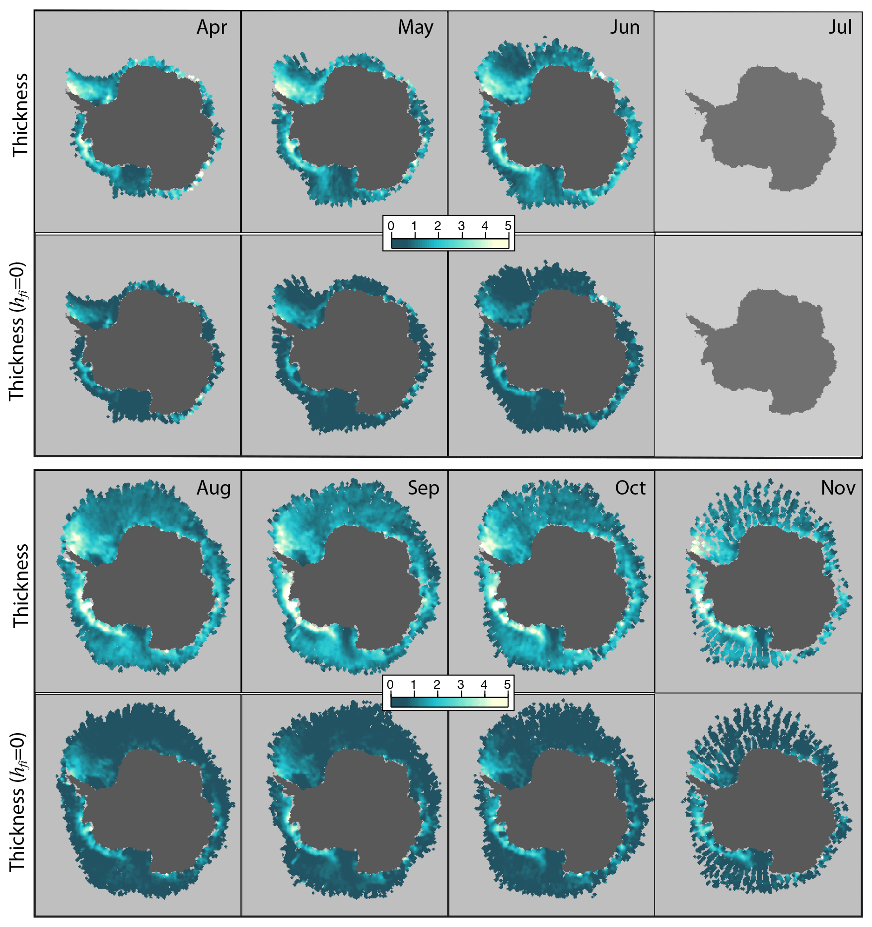
Figure 8Monthly composites of calculated ice thicknesses: (a) hi, using snow depth from freeboard differences , and (b) , assuming zero ice freeboard, i.e., hfs=hf, for the period between April and November 2019. (25 km grid; in meters).

Figure 9Monthly distributions of calculated ice thicknesses: (a) hi, using snow depth from freeboard differences , and (b) , assuming zero ice freeboard, i.e., hfs=hf, for the period between April and November 2019. Their monthly means are compared in (c) (distributions are normalized).
5.2 Monthly ice thickness (April–November)
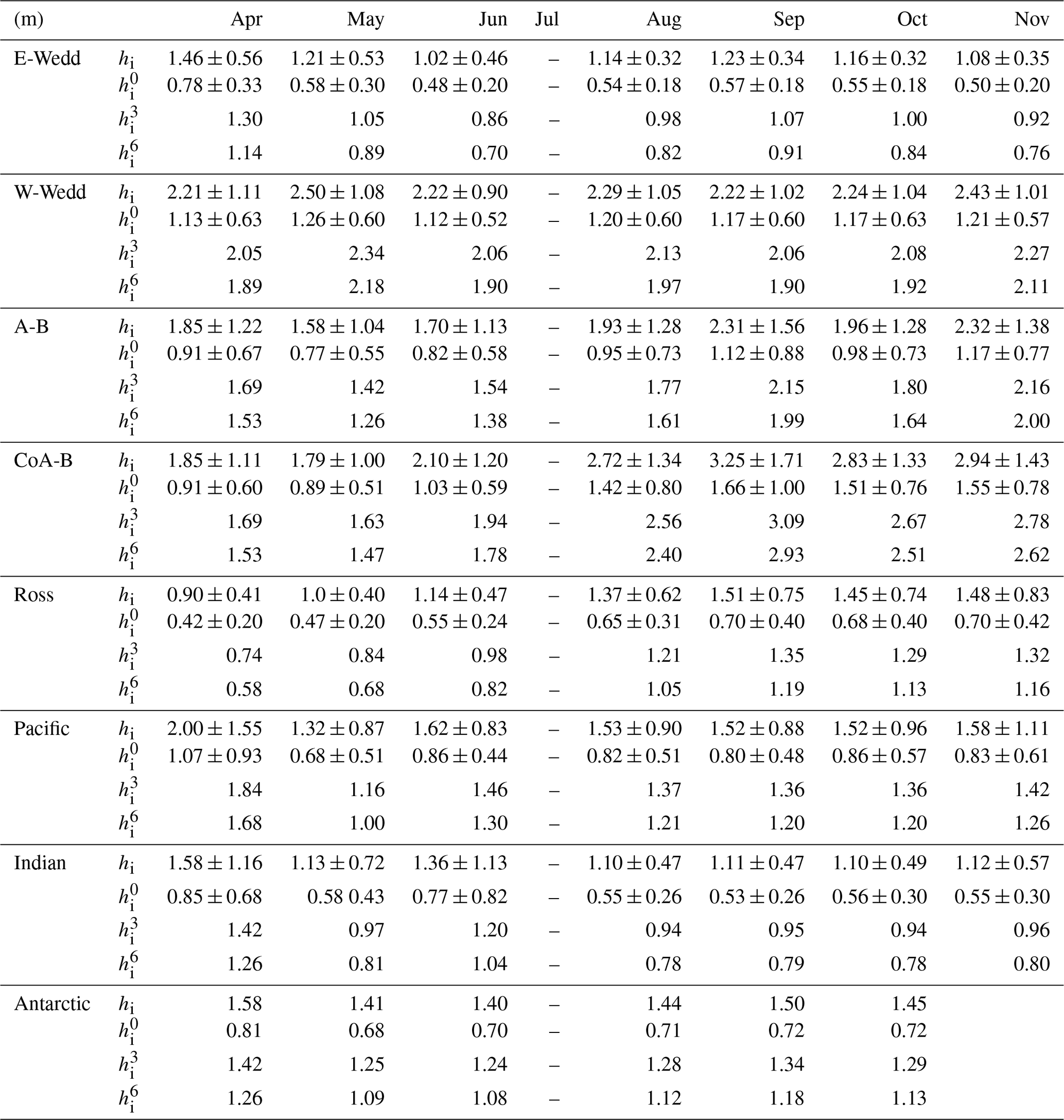
The monthly thickness composites (hi and ) and their distributions are shown in Figs. 8 and 9, respectively, and the numerical averages are in Table 2. Again, the spatial patterns of the thickness composites are very similar to that of the freeboards and snow depth, and so here we note only the features and differences.
As expected, the thickest ice is found in the W-Wedd sector (mean 2.50 ± 1.08 m in May) and the CoA-B sector (3.25 ± 1.71 m in September). These are also sectors where the highest snow depths are found. The thinnest ice is in the Ross (0.90 ± 0.41 m in April) and E-Wedd (< 1.5 m for all months) sectors. The tongue of lower ice thickness in the Ross sector (Fig. 8) is a clear signature of the outflow of thin and young ice produced in the Ross Sea polynyas. Similarly, for the E-Wedd sector, the large expanse of thinner seasonal ice is also evident. Consistent thinning towards the ice margins is seen almost everywhere and in all months.
The seasonal cycle of ice thickness is surprisingly weak. Seasonal increases in the monthly mean ice thickness are only evident in the A-B and CoA-B sectors. Notably, in the CoA-B sector, the increase in ∼ 1 m (from 1.85 ± 1.11 m in April to 2.94 ± 1.43 m in November) over the 8 months discussed earlier, is connected to coastal ice convergence (the mechanical redistribution of thin to thicker ice) associated with persistent on-shore wind pattern in 2019. In all other sectors, we find either decreases or relatively unchanging thicknesses (i.e., weak seasonality) from April to November.

Figure 10Comparison of seasonal ice thickness calculated with δ=0, 3 and 6 cm, and assuming zero ice freeboard (i.e., hfs=hf) with shipborne measurements in Worby et al. (2008).
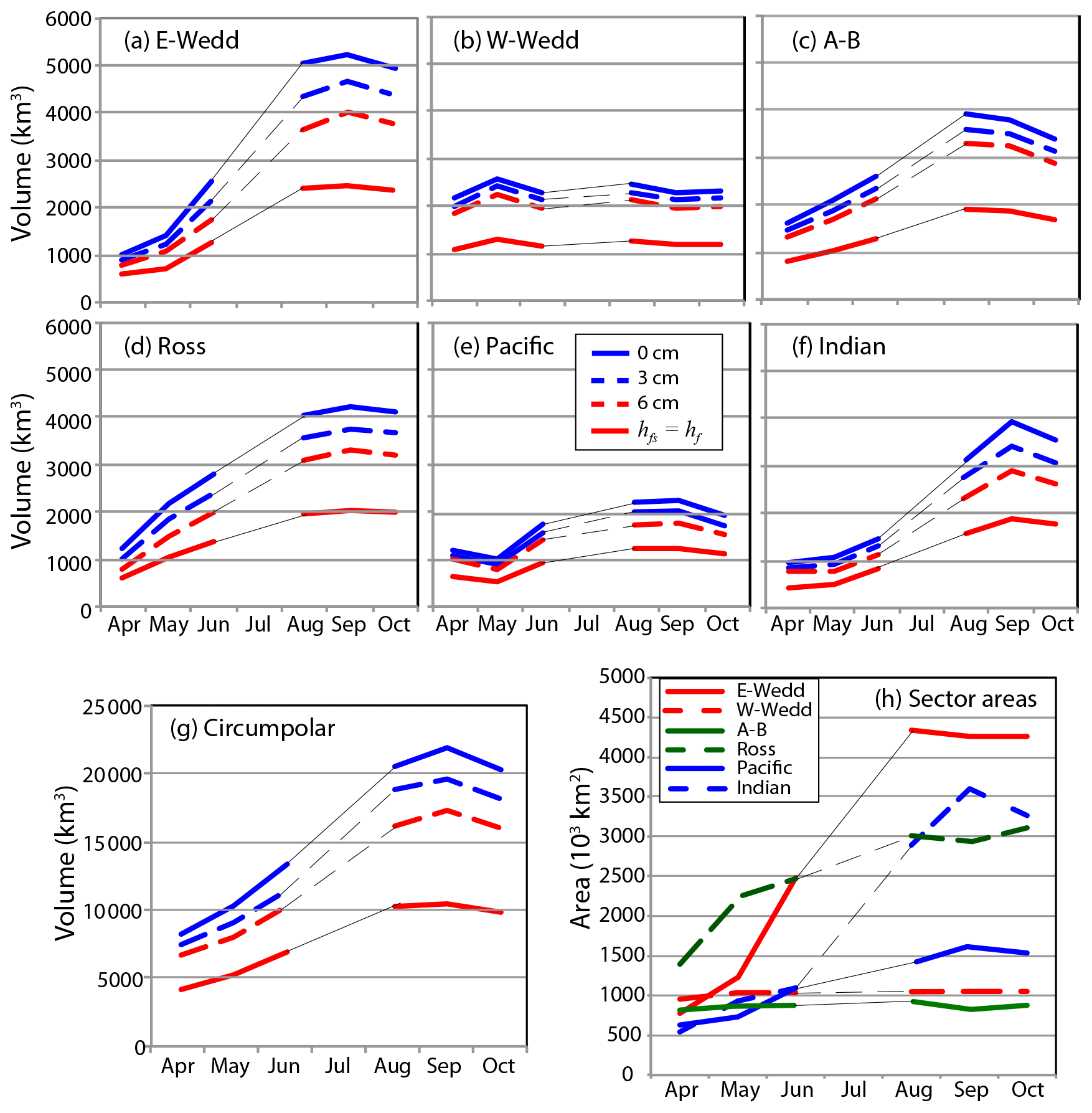
Figure 11Evolution of the volume and area of the Antarctic sea ice cover between April and October 2019.
There are no seasonally and regionally diverse data sets from field observations that could be used to assess the large-scale satellite retrievals. Field observations of ice thickness are from two main sources: shipborne observations and mechanical drilling profiles. The most extensive compilation of Antarctic ice thickness is from the ASPeCt database reported in Worby et al. (2008), it contains data from 83 voyages and 2 helicopter flights for the period 1980–2005. Figure 10 compares our thickness estimates with the ASPeCt data summarized in Worby et al. (2008). For all seasons and sectors, the overall ice thickness in the ASPeCt data (circles in Fig. 10) is less than half the mean thickness in our estimates (solid blue line). There are two reasons these data sets are not comparable: (1) the ASPeCt data are biased towards thin and level ice types and (2) few of the ASPeCt data have been collected at a similar time and location; indeed, ASPeCt observations of the coastal southern Bellingshausen and Amundsen seas in spring are not available. Underway shipboard observations made while traversing the pack ice (in ASPeCt database) favor sampling the thinner end of the thickness distribution due to physical, navigational, and logistical constraints. Hence, the sample population in the ASPeCt database is not likely to represent the regional statistics needed for assessment of the satellite retrievals. Drilling data may be more comparable, as they provide a better sampling of the thickness distribution and of ice thick enough to stand on, but this limits the sampling of very thin ice. However, almost all drilling data to date are from thinner floes (Ozsoy-Cicek et al., 2013) and the thickest ice is often avoided. Even though drilling measurements have provided locations on where one should expect thicker ice (e.g., Williams et al., 2015; Lange and Eicken, 1991; Massom et al., 2001), they rarely provide averages at spatial scales compatible with satellite averages.
Ice thickness estimates from Operation IceBridge provide averages at a larger scale, but they are still limited in terms of seasonal coverage. In an examination of 3 years of OIB ice thickness, Kwok and Kacimi (2018) report October ice thicknesses that range from 2.40 to 2.60 m over a transect across the Weddell Sea (from the tip of the Antarctic Peninsula to Cape Norvegia). This is more compatible with the averages in the W-Wedd sector in Fig. 10a (solid blue line). In a north–south OIB transect of the Ross Sea in November, Tian et al. (2020) found ice thicknesses between 0.48 and 0.99 m, again more compatible with that seen in Fig. 10d (solid blue line). In any case, a more exhaustive evaluation of the present data set remains a challenge.
Table 3Monthly mean (standard deviation) of estimated ice thickness: (1) hi, with derived snow depth (hi); (2) , assuming hfs=hf; (3) , with δ=3 cm; and (4) , with δ=6 cm.
5.3 Are the thickness estimates high?
In sectors where there is predominantly seasonal ice (Ross, Pacific, Indian, E-Wedd) the ice thickness in the early winter months of April and May, at close to ∼ 1.5 m, seems to be too high. In these sectors, the growth of 1 m of sea ice in the 1–2 months between freeze-up (in February, March) and April–May is unlikely. With ice drift that is largely seaward and divergent during these months (Fig. 5), the only two processes that contribute significantly to increases in thickness are basal growth and snow ice formation. In the short 1–2 months from freeze-up, basal thermodynamic growth of 1 m is unlikely given the oceanic conditions (ocean heat flux in a weakly stratified ocean compared to the Arctic). Additionally, it would require high snowfall rates to create a significant thickness of snow ice in that amount of time. Thus, this points strongly to biases in the CS-2 freeboards, as the estimated thicknesses are highly sensitive to these biases (due to large 3 : 1 contrast between ice and snow densities in Eq. 11).
Clearly, if ice freeboard were zero everywhere, then (Eq. 12) would be the best estimate of ice thickness given measurements of total freeboard. However, this is unlikely to be the case, especially in the W-Wedd and CoA-B sectors where thicker ice is known to be present (see the discussion above). If there were a large-scale bias in the CS-2 freeboards (assuming the processes that contribute to the radar biases are the same everywhere) then areas with the lowest CS-2 freeboards provide a rough guidance on the magnitude of that bias. In the four sectors of largely seasonal ice (Ross, Pacific, Indian, E-Wedd), the sector-averaged CS-2 freeboards have the lowest values and low seasonal variability that ranges from 5.86 ± 2.50 cm (minimum) to 10.3 ± 3.67 cm for all months. This suggests a bias (δ) of ∼ 6 cm if we assumed that early season ice freeboards have to be near zero. This value can be compared to reported biases from different studies; some examples are listed below.
-
The thickness of the high-salinity basal layer of 0–3 cm (> 10) reported by Massom et al. (1997).
-
Suggested adjustment (δ) of ∼ 7 cm on first-year ice in the Arctic based on a scattering study using profiles of basal salinities (Nandan et al., 2017, 2020).
-
Observed CS-2 biases of up to 8 cm in the Weddell Sea in an assessment of the IceBridge- and CS-2-derived ice thicknesses (Kwok and Kacimi, 2018).
-
The 3.4–4.5 cm bias from the linear regressions estimated in Sect. 4.3.
In the following section, we examine the sensitivity of thickness and volume if these biases were generally representative over the entire ice cover.
5.4 Thickness and volume estimates with and without adjustments
As discussed above, sea ice would be too thick using the CS-2 freeboards directly and too thin if ice freeboard were assumed to be zero everywhere. Guided by the potential range of CS-2 freeboard biases above, we calculate the regional thickness and volume of the Antarctic ice cover with adjustments (δ) of 3 and 6 cm (Eq. 13) to assess the variability of sector ice volume between the two extremes of thicknesses (i.e., hi and ) over the winter of 2019. The monthly composites and the sector thicknesses (with δ=0, 3, 6 cm) can be seen in Fig. 10 and Table 3, and the monthly ice volumes are shown in Fig. 11.
The adjustments to CS-2 freeboards, as expected, lower the thickness (5 cm per 1 cm of adjustment, based on Eq. 10); at δ=6 cm the sector mean would be reduced by 0.32 m. The impact is higher, in terms of fractional change in total thickness, in sectors with thinner ice (e.g., E-Wedd). The range of thicknesses in Fig. 10 gives us at least an indication of the potential range of variability between assuming zero ice freeboard and the rough estimates of δ (applied as a sector-wide bias). Even though current knowledge does not allow us to adjust individual thickness retrievals, these large-scale adjustments likely provide a better estimate than those calculated using hi or .
The end-of-season ice volume in each sector is proportional to the area production (Fig. 11h) with the largest ice volume in the E-Wedd sector. This, of course, is not the ice volume production in a particular sector. In order to calculate seasonal ice production, one has to account for volume exchanges at the sector boundaries and volume lost to melt at the ice edge. Of interest here is the ice volume and its sensitivity to δ. At the end of the season, the difference in total Antarctic ice volume between assuming δ=0 and hfs=hf is ∼ 10 000 km3, or one-third of the total volume. Adjustments with δ=3 and δ=6 cm reduce the differences by ∼ 2000 and 4000 km3, respectively. As with ice thickness, in sectors where the ice is thicker (W-Wedd, Fig. 10), the fractional changes are smaller. An adjustment of 6 cm gives a circumpolar ice volume of 15 600 km3 in October, for an average thickness of ∼ 1.13 m.
These volume estimates can be compared to volume estimates from ICESat freeboards. Using AMSR snow depths, Zwally et al. (2008) estimated the average October–November (2004 and 2005) Weddell Sea ice volume to be ∼ 8750 km3, comparable to our 2019 estimate of 7264 km3 (without any adjustments). Here, differences are expected as the efficacy of the AMSR snow depths has yet to be demonstrated.
Assuming snow depth to be the total freeboard (i.e., zero ice freeboard), Kurtz and Markus (2012) estimated an average circumpolar ice volume of 11 111 km3 in the spring (2003 through 2008) with an average thickness of 0.83 m; this can be compared to our October estimate of 10 062 km3 and 0.72 m using the same assumption. Our lower volume estimates may be partly attributable to the retreat in Antarctic ice coverage (Parkinson, 2019) since the ICESat mission of > 106 km2. With the same assumption of zero ice freeboard, the change of 0.11 m between ICESat and IS-2 in 2019 may be of interest, but this is more of an indication of decrease in total freeboard rather than an actual change in ice thickness.
In this study, we offer a view of the Antarctic sea ice cover from lidar (ICESat-2) and radar (CryoSat-2) altimetry. This is a first joint examination of the IS-2 and CS-2 freeboards, the snow depth derived from their differences, and the calculated sea ice thickness and volume. Our analysis spans an 8-month winter between 1 April and 16 November 2019. We characterize the behavior of the circumpolar ice cover in seven geographic sectors. The limitations in our current knowledge in the retrieval of snow depth, thickness, and volume are addressed. Below we highlight some of the results and discuss future opportunities for validation and assessment of this retrieval approach.
-
The highest freeboards are seen in the CoA-B and W-Wedd sectors. The remarkable ice convergence due to on-shore wind and ice drift along the coastal Amundsen Sea, associated with the depth, location, and persistence of Amundsen Sea Low pattern, is captured in the correlated changes in IS-2 and CS-2 freeboards with extremes of 54.0 ± 32.5 cm (in September) and 15.6 ± 6.83 cm (in October), respectively, and derived thickness of 3.25 ± 1.71 m (in September). The multiyear ice in the W-Wedd sector, as expected, also stands out with high freeboards and thickness (sector mean thickness of 2.50 ± 1.08 m in May).
-
The lowest freeboards, snow depths, and thicknesses are seen in the proximity of the Ross Sea and Ronne polynyas. In the Ross Sea sector, the lowest sector-averaged IS-2 and CS-2 freeboards of 13.8 ± 6.45 cm and 6.78 ± 2.81 cm, respectively, can be contrasted with those in the CoA-B and W-Wedd given above.
-
Variability in CS-2 freeboards is low. Hence, the Antarctic snow depth estimates are highly correlated with IS-2 freeboards, with the IS-2 freeboard explaining > 90 % of the variance in snow depth. Our results suggest that more than 60 %–70 % of the IS-2 freeboard is snow.
-
In 2019, the observed seasonality in the sector-averaged freeboards, snow depth, and thickness is surprisingly weak. These sector averages do not follow the expected seasonal increases due to ice growth and snow accumulation seen in the Arctic. We attribute this to the mixture of competing processes (snowfall, snow redistribution, snow ice formation, ice deformation, and basal growth and melt) in different parts of the divergent Antarctic ice cover and the continuous export of sea ice to the margins, where they subsequently melt.
-
Evidence points to biases in CS-2 freeboards that are associated with displacement of the retracking points to a height above the snow–ice interface, resulting in snow depths that are too low and ice thicknesses that are too high in the present retrievals. Based on field measurements, a contributing source to the bias is the salinity at the base of the snow layer due to wicking and flooding; the physical basis of expected biases in CS-2 freeboards from basal-layer salinity is sound. The question is the range of the biases and whether a correction factor could be applied for retrievals at the highest spatial resolution.
-
Our calculations show the sector-scale variability of snow depth, thickness and computed ice volume given biases of 3 and 6 cm in radar freeboard and assuming zero ice freeboard. At the sector scale, the adjusted estimates seem to be more credible, although better assessment of these parameter awaits better field measurements. An adjustment of 3–6 cm gives a circumpolar ice volume of 17 900–15 700 km3 in October, for an average thickness of ∼ 1.29–1.13 m.
-
Validation of Antarctic sea ice parameters remains a challenge. There are no seasonally and regionally diverse data sets from field records that could be used to assess the large-scale satellite retrievals, especially in areas that are inaccessible to ships. The overall ice thickness in the ASPeCt data in all seasons and locations are less than half the mean thickness in the present data and points to the sampling biases from underway shipboard observations. There is an urgent need for sustained and extensive field measurements.
The present analysis, however, is only a first step in the examination of the Antarctic ice cover using both the IS-2 and CS-2 altimeters. There are many aspects of data quality, some of which will only be revealed by assessment with data acquired and processed by dedicated airborne campaigns (e.g., NASA's Operation IceBridge), field programs, and when a longer IS-2/CS-2 time series becomes available. An adjustment of the CS-2 orbits (by ESA), CRYO2ICE, to provide improved coincidence in space–time sampling of the two altimeters has been successfully implemented. We anticipate that the data acquired by CRYO2ICE will provide a crucial and valuable data set not only for understanding current retrievals but also for the design of future instruments tasked to understand the development of the Arctic and Antarctic sea ice cover.
The ASPeCt database can be accessed at https://doi.org/10.4225/15/59a8bd4b05d10 (Heil, 2017). AMSR ice concentrations are available at https://doi.org/10.5067/TRUIAL3WPAUP (Markus et al., 2018). CS-2 data are from the ESA data portal (https://earth.esa.int/web/guest/-/cryosat-products, ESA, 2019a, b). The ICESat-2 ATL10 data sets used herein are available at https://doi.org/10.5067/ATLAS/ATL10.002 (Kwok et al., 2019d).
SK and RK designed the experiments and carried them out. Both SK and RK contributed to the preparation of the figures and manuscript.
The authors declare that they have no conflict of interest.
We thank the editor (Petra Heil) and the reviewers (Rachel Tilling and one anonymous reviewer) for their careful reading of the submission and offering of useful comments and suggestions, which helped improve the manuscript. We also thank the International Space Science Institute (ISSI) for supporting and hosting the useful workshops on Satellite Remote Sensing of Antarctic sea ice held in Bern, Switzerland, over the past decade.
Part of this research was carried out at the Jet Propulsion Laboratory, California Institute of Technology, under a contract with the National Aeronautics and Space Administration and funded through the internal Research and Technology Development program, Earth 2050.
This paper was edited by Petra Heil and reviewed by Rachel Tilling and one anonymous referee.
Andreas, E. L. and Claffey, K. J.: Air-Ice Drag Coefficients in the Western Weddell Sea .1. Values Deduced from Profile Measurements, J. Geophys. Res., 100, 4821–4831, https://doi.org/10.1029/94jc02015, 1995.
Comiso, J. C. and Nishio, F.: Trends in the sea ice cover using enhanced and compatible AMSR-E, SSM/I, and SMMR data, J. Geophys. Res., 113, C02S07, https://doi.org/10.1029/2007jc004257, 2008.
Cullather, R. I., Bromwich, D. H., and Van Woert, M. L.: Spatial and temporal variability of Antarctic precipitation from atmospheric methods, J Climate, 11, 334–367, https://doi.org/10.1175/1520-0442(1998)011<0334:Satvoa>2.0.Co;2, 1998.
Drucker, R., Martin, S., and Kwok, R.: Sea ice production and export from coastal polynyas in the Weddell and Ross Seas, Geophys. Res. Lett., 38, L17502, https://doi.org/10.1029/2011GL048668, 2011.
European Space Agency (ESA): L1b SAR Precise Orbit. Baseline D, https://doi.org/10.5270/CR2-2cnblvi, 2019a.
European Space Agency (ESA): L1b SARin Precise Orbit. Baseline D, https://doi.org/10.5270/CR2-u3805kw, 2019b.
Giles, K. A., Laxon, S. W., and Worby, A. P.: Antarctic sea ice elevation from satellite radar altimetry, Geophys. Res. Lett., 35, L03503 https://doi.org/10.1029/2007gl031572, 2008.
Heil, P.: ASPeCt Sea Ice Data from the SIPEX Voyage of the Aurora Australis in 2007–2008, Ver. 1, Australian Antarctic Data Centre, https://doi.org/10.4225/15/59a8bd4b05d10, 2017.
Hobbs, W. R., Bindoff, N. L., and Raphael, M. N.: New Perspectives on Observed and Simulated Antarctic Sea Ice Extent Trends Using Optimal Fingerprinting Techniques, J. Clim., 28, 1543–1560, https://doi.org/10.1175/JCLI-D-14-00367.1, 2015.
Holland, P. R. and Kwok, R.: Wind-driven trends in Antarctic sea-ice drift, Nat. Geosci., 5, 872–875, https://doi.org/10.1038/NGEO1627, 2012.
Holland, P. R., Bruneau, N., Enright, C., Losch, M., Kurtz, N. T., and Kwok, R.: Modeled Trends in Antarctic Sea Ice Thickness, J. Clim., 27, 3784–3801, https://doi.org/10.1175/JCLI-D-13-00301.1, 2014.
Jeffries, M. O., Krouse, H. R., Hurst-Cushing, B., and Maksym, T.: Snow-ice accretion and snow-cover depletion on Antarctic first-year sea-ice floes, Ann. Glaciol., 33, 51–60, https://doi.org/10.3189/172756401781818266, 2001.
Kurtz, N. T. and Markus, T.: Satellite observations of Antarctic sea ice thickness and volume, J. Geophys. Res., 117, C08025, https://doi.org/10.1029/2012jc008141, 2012.
Kwok, R.: Simulated effects of a snow layer on retrieval of CryoSat-2 sea ice freeboard, Geophys. Res. Lett., 41, 5014–5020, https://doi.org/10.1002/2014gl060993, 2014.
Kwok, R. and Cunningham, G. F.: Variability of Arctic sea ice thickness and volume from CryoSat-2, Phil. Trans. R. Soc. A, 373, 20140157, https://doi.org/10.1098/rsta.2014.0157, 2015.
Kwok, R. and Kacimi, S.: Three years of sea ice freeboard, snow depth, and ice thickness of the Weddell Sea from Operation IceBridge and CryoSat-2, The Cryosphere, 12, 2789–2801, https://doi.org/10.5194/tc-12-2789-2018, 2018.
Kwok, R., Spreen, G., and Pang, S.: Arctic sea ice circulation and drift speed: Decadal trends and ocean currents, J. Geophys. Res., 118, 2408–2425, https://doi.org/10.1002/jgrc.20191, 2013.
Kwok, R., Pang, S. S., and Kacimi, S.: Sea ice drift in the Southern Ocean: Regional patterns, variability, and trends, Elementa Science of the Anthropocene, 5, 32, https://doi.org/10.1525/elementa.226, 2017.
Kwok, R., Cunningham, G. F., Hancock, D. W., Ivanoff, A., and Wimert, J. T.: Ice, Cloud, and Land Elevation Satellite-2 Project: Algorithm Theoretical Basis Document (ATBD) for Sea Ice Products, https://icesat-2.gsfc.nasa.gov/science/data_products (last access: 15 January 2020), 2019a.
Kwok, R., Cunningham, G. F., Markus, T., Hancock, D., Morison, J., Palm, S., Farrell, S., Ivanoff, A., and Wimert, J.: ATLAS/ICESat-2 L3A Sea Ice Height, Version 1, Boulder, Colorado USA, NSIDC: National Snow and Ice Data Center, https://doi.org/10.5067/ATLAS/ATL07.001, 2019b.
Kwok, R., Kacimi, S., Markus, T., Kurtz, N. T., Studinger, M., Sonntag, J. G., Manizade, S. S., Boisvert, L. N., and Harbeck, J. P.: ICESat-2 Surface Height and Sea Ice Freeboard Assessed With ATM Lidar Acquisitions From Operation IceBridge, Geophys. Res. Lett., 46, 11228–11236, https://doi.org/10.1029/2019gl084976, 2019c.
Kwok, R., Cunningham, G., Markus, T., Hancock, D., Morison, J. H., Palm, S. P., Farrell, S. L., Ivanoff, A., Wimert, J., and the ICESat-2 Science Team: ATLAS/ICESat-2 L3A Sea Ice Freeboard, Version 2, Boulder, Colorado USA, NASA National Snow and Ice Data Center Distributed Active Archive Center, https://doi.org/10.5067/ATLAS/ATL10.002, 2019d.
Kwok, R., Kacimi, S., Webster, M. A., Kurtz, N. T., and Petty, A. A.: Arctic Snow Depth and Sea Ice Thickness From ICESat-2 and CryoSat-2 Freeboards: A First Examination, J. Geophys. Res. , 125, e2019JC016008, https://doi.org/10.1029/2019jc016008, 2020.
Lange, M. A. and Eicken, H.: The Sea Ice Thickness Distribution in the Northwestern Weddell Sea, J. Geophys. Res., 96, 4821–4837, https://doi.org/10.1029/90jc02441, 1991.
Mahlstein, I., Gent, P. R., and Solomon, S.: Historical Antarctic mean sea ice area, sea ice trends, and winds in CMIP5 simulations, J. Geophys. Res., 118, 5105–5110, https://doi.org/10.1002/jgrd.50443, 2013.
Maksym, T. and Markus, T.: Antarctic sea ice thickness and snow-to-ice conversion from atmospheric reanalysis and passive microwave snow depth, J. Geophys. Res., 113, C02s12, https://doi.org/10.1029/2006jc004085, 2008.
Markus, T., Comiso, J. C., and Meier, W. N.: AMSR-E/AMSR2 Unified L3 Daily 25 km Brightness Temperatures & Sea Ice Concentration Polar Grids, Version 1, Boulder, Colorado USA, NASA National Snow and Ice Data Center Distributed Active Archive Center, https://doi.org/10.5067/TRUIAL3WPAUP, 2018.
Massom, R. A., Drinkwater, M. R., and Haas, C.: Winter snow cover on sea ice in the Weddell Sea, J. Geophys. Res., 102, 1101–1117, https://doi.org/10.1029/96jc02992, 1997.
Massom, R. A., Lytle, V. I., Worby, A. P., and Allison, I.: Winter snow cover variability on East Antarctic sea ice, J. Geophys. Res., 103, 24837–24855, https://doi.org/10.1029/98jc01617, 1998.
Massom, R. A., Eicken, H., Haas, C., Jeffries, M. O., Drinkwater, M. R., Sturm, M., Worby, A. P., Wu, X. R., Lytle, V. I., Ushio, S., Morris, K., Reid, P. A., Warren, S. G., and Allison, I.: Snow on Antarctic Sea ice, Rev. Geophys., 39, 413–445, https://doi.org/10.1029/2000rg000085, 2001.
Massonnet, F., Mathiot, P., Fichefet, T., Goosse, H., Beatty, C. K., Vancoppenolle, M., and Lavergne, T.: A model reconstruction of the Antarctic sea ice thickness and volume changes over 1980–2008 using data assimilation, Ocean Model., 64, 67–75, https://doi.org/10.1016/j.ocemod.2013.01.003, 2013.
Nandan, V., Geldsetzer, T., Yackel, J., Mahmud, M., Scharien, R., Howell, S., King, J., Ricker, R., and Else, B.: Effect of Snow Salinity on CryoSat-2 Arctic First-Year Sea Ice Freeboard Measurements, Geophys. Res. Lett., 44, 10419–10426, https://doi.org/10.1002/2017gl074506, 2017.
Nandan, V., Scharien, R. K., Geldsetzer, T., Kwok, R., Yackel, J. J., Mahmud, M. S., Rosel, A., Tonboe, R., Granskog, M., Willatt, R., Stroeve, J., Nomura, D., and Frey, M.: Snow Property Controls on Modeled Ku-Band Altimeter Estimates of First-Year Sea Ice Thickness: Case Studies From the Canadian and Norwegian Arctic, IEEE J. Sel. Top. Appl., 13, 1082–1096, https://doi.org/10.1109/jstars.2020.2966432, 2020.
Neumann, T. A., Martino, A. J., Markus, T., Bae, S., Bock, M. R., Brenner, A. C., Brunt, K. M., Cavanaugh, J., Fernandes, S. T., Hancock, D. W., Harbeck, K., Lee, J., Kurtz, N. T., Luers, P. J., Luthcke, S. B., Magruder, L., Pennington, T. A., Ramos-Izquierdo, L., Rebold, T., Skoog, J., and Thomas, T. C.: The Ice, Cloud, and Land Elevation Satellite – 2 mission: A global geolocated photon product derived from the Advanced Topographic Laser Altimeter System, Remote Sens. Environ., 233, 111325, https://doi.org/10.1016/j.rse.2019.111325, 2019.
Ozsoy-Cicek, B., Ackley, S., Xie, H., Yi, D., and Zwally, J.: Sea ice thickness retrieval algorithms based on in situ surface elevation and thickness values for application to altimetry, J. Geophys. Res., 118, 3807–3822, https://doi.org/10.1002/jgrc.20252, 2013.
Parkinson, C. L.: A 40-y record reveals gradual Antarctic sea ice increases followed by decreases at rates far exceeding the rates seen in the Arctic, P. Natl. Acad. Sci. USA, 116, 14414–14423, https://doi.org/10.1073/pnas.1906556116, 2019.
Polvani, L. M. and Smith, K. L.: Can natural variability explain observed Antarctic sea ice trends? New modeling evidence from CMIP5, Geophys. Res. Lett., 40, 3195–3199, https://doi.org/10.1002/grl.50578, 2013.
Tian, L., Xie, H., Ackley, S. F., Tang, J., Mestas-Nuñez, A. M., and Wang, X.: Sea-ice freeboard and thickness in the Ross Sea from airborne (IceBridge 2013) and satellite (ICESat 2003–2008) observations, Ann. Glaciol., 1–16, https://doi.org/10.1017/aog.2019.49, 2020.
Toyota, T., Massom, R., Lecomte, O., Nomura, D., Heil, P., Tamura, T., and Fraser, A. D.: On the extraordinary snow on the sea ice off East Antarctica in late winter, 2012, Deep-Sea Res. Pt. II, 131, 53–67, https://doi.org/10.1016/j.dsr2.2016.02.003, 2016.
Turner, J., Hosking, J. S., Bracegirdle, T. J., Marshall, G. J., and Phillips, T.: Recent changes in Antarctic Sea Ice, Phil. Trans. R. Soc. A, 373, 20140163, https://doi.org/10.1098/rsta.2014.0163, 2015.
Ulaby, F. T., Moore, R. K., and Fung, A. K.: Microwave remote sensing: from theory to applications, Artech House, Norwood, MA, 1986.
Vaughan, D. G., Comiso, J., Allison, I., Carrasco, G., Kaser, G., Kwok, R., Mote, P., Murray, T., Paul, F., Ren, J., Rignot, E., Solomina, O., Steffen, K., and Zhang, T.: Observations: Cryosphere, in: Climate Change 2013: The Physical Science Basis, Contribution of Working Group I to the Fifth Assessment Report of the Intergovernmental Panel on Climate Change, edited by: Stocker, T. F., Qin, D., Plattner, G.-K., Tignor, M., Allen, S. K., Boschung, J., Nauels, A., Xia, Y., Bex, V., and Midgley, P. M., Cambridge University Press, Cambridge, UK, 317–382, 2013.
Vernet, M., Geibert, W., Hoppema, M., Brown, P. J., Haas, C., Hellmer, H. H., Jokat, W., Jullion, L., Mazloff, M., Bakker, D. C. E., Brearley, J. A., Croot, P., Hattermann, T., Hauck, J., Hillenbrand, C. D., Hoppe, C. J. M., Huhn, O., Koch, B. P., Lechtenfeld, O. J., Meredith, M. P., Naveira Garabato, A. C., Nöthig, E. M., Peeken, I., Rutgers van der Loeff, M. M., Schmidtko, S., Schröder, M., Strass, V. H., Torres-Valdés, S., and Verdy, A.: The Weddell Gyre, Southern Ocean: Present Knowledge and Future Challenges, Rev. Geophys., 57, 623–708, https://doi.org/10.1029/2018rg000604, 2019.
Willatt, R., Laxon, S., Giles, K., Cullen, R., Haas, C., and Helm, V.: Ku-band radar penetration into snow cover Arctic sea ice using airborne data, Ann. Glaciol., 52, 197–205, https://doi.org/10.3189/172756411795931589, 2011.
Willatt, R. C., Giles, K. A., Laxon, S. W., Stone-Drake, L., and Worby, A. P.: Field Investigations of Ku-Band Radar Penetration Into Snow Cover on Antarctic Sea Ice, IEEE Trans. Geosci. Remote Sens., 48, 365–372, https://doi.org/10.1109/Tgrs.2009.2028237, 2010.
Williams, G., Maksym, T., Wilkinson, J., Kunz, C., Murphy, C., Kimball, P., and Singh, H.: Thick and deformed Antarctic sea ice mapped with autonomous underwater vehicles, Nat. Geosci., 8, 61–67, https://doi.org/10.1038/Ngeo2299, 2015.
Winebrenner, D. P., Nelson, E. D., Colony, R., and West, R. D.: Observation of Melt Onset on Multiyear Arctic Sea-Ice Using the Ers-1 Synthetic-Aperture-Radar, J. Geophys. Res., 99, 22425–22441, https://doi.org/10.1029/94jc01268, 1994.
Worby, A. P., Geiger, C. A., Paget, M. J., Van Woert, M. L., Ackley, S. F., and DeLiberty, T. L.: Thickness distribution of Antarctic sea ice, J. Geophys. Res., 113, C05S92, https://doi.org/10.1029/2007jc004254, 2008.
Xie, H. J., Tekeli, A. E., Ackley, S. F., Yi, D. H., and Zwally, H. J.: Sea ice thickness estimations from ICESat Altimetry over the Bellingshausen and Amundsen Seas, 2003–2009, J. Geophys. Res., 118, 2438–2453, https://doi.org/10.1002/jgrc.20179, 2013.
Yi, D. H., Zwally, H. J., and Robbins, J. W.: ICESat observations of seasonal and interannual variations of sea-ice freeboard and estimated thickness in the Weddell Sea, Antarctica (2003–2009), Ann. Glaciol., 52, 43–51, https://doi.org/10.3189/172756411795931480, 2011.
Zhang, J.: Modeling the Impact of Wind Intensification on Antarctic Sea Ice Volume, J. Clim., 27, 202–214, https://doi.org/10.1175/jcli-d-12-00139.1, 2014.
Zunz, V., Goosse, H., and Massonnet, F.: How does internal variability influence the ability of CMIP5 models to reproduce the recent trend in Southern Ocean sea ice extent?, The Cryosphere, 7, 451–468, https://doi.org/10.5194/tc-7-451-2013, 2013.
Zwally, H. J., Yi, D. H., Kwok, R., and Zhao, Y. H.: ICESat measurements of sea ice freeboard and estimates of sea ice thickness in the Weddell Sea, J. Geophys. Res., 113, C02S15, https://doi.org/10.1029/2007jc004284, 2008.