Mapping the age of ice of Gauligletscher combining surface radionuclide contamination and ice flow modeling

In the 1950s and 1960s, specific radionuclides were released into the atmosphere as a result of nuclear weapons testing. This radioactive fallout left its signature on the accumulated layers of glaciers worldwide, thus providing a tracer for ice particles traveling within the gravitational ice flow and being released into the ablation zone. For surface ice dating purposes, we analyze here the activity of ²³⁹Pu, ²⁴⁰Pu and ²³⁶U radionuclides derived from more than 200 ice samples collected along five flowlines at the surface of Gauligletscher, Switzerland. It was found that contaminations appear band-wise along most of the sampled lines, revealing a V-shaped profile consistent with the ice flow field already observed. Similarities to activities found in ice cores permit the isochronal lines at the glacier from 1960 and 1963 to be identified. Hence this information is used to fine-tune an ice flow/mass balance model, and to accurately map the age of the entire glacier ice. Our results indicate the strong potential for combining radionuclide contamination and ice flow modeling in two different ways. First, such tracers provide unique information on the long-term ice motion of the entire glacier (and not only at its surface), and on the long-term mass balance, and therefore offer an extremely valuable data tool for calibrating ice flows within a model. Second, the dating of surface ice is highly relevant when conducting “horizontal ice core sampling”, i.e., when taking chronological samples of surface ice from the distant past, without having to perform expensive and logistically complex deep ice-core drilling. In conclusion, our results show that an airplane which crash-landed on the Gauligletscher in 1946 will likely soon be released from the ice close to the place where pieces have emerged in recent years, thus permitting the prognosis given in an earlier model to be revised considerably.

1 Introduction

Climate change is expected to bring about the massive retreat of glaciers worldwide (e.g., Marzeion et al., 2018) with important consequences for hydropower production (Schaefli et al., 2019), the tourism economy (Wiesmann et al., 2005) or in terms of sea level rise (Mengel et al., 2018). It is therefore of major interest to model the future extents of glaciers in order to anticipate the projected change as accurately as possible. To meet the need for prediction tools, numerical models combining ice flow and surface mass balance have been developed at different levels of complexity, from flowline models based on mechanical approximations (e.g., Wallinga and van de Wal, 1998) to three-dimensional models based on full Stokes equations (e.g., Gagliardini et al., 2013). A common difficulty in setting up sophisticated models is the lack of data to simultaneously constrain the key parameters that control the mass balance, the ice deformation and the basal conditions; this can be a source of major model uncertainties (Gillet-Chaulet et al., 2012). For instance, both mass balance measurements and ice velocities observed at the glacier surface are generally available only for the ablation area and for the recent past. As a result models rely essentially on sparse data that ignore the dynamics of the upper glacier part and rarely integrate long time series that account for the decadal-scale variability of the ice movements (glaciers were in general thicker and therefore faster in the past). Another important limitation is that models rarely integrate data on the basal motion at the bedrock, for reasons of inaccessibility (Vincent and Moreau, 2016).

One way to tackle this issue is to include Lagrangian information on ice particles traveling from the accumulation to the ablation zone whenever we have proxy data to track their trajectories. The surface ice is expected to be young near the equilibrium line altitude and to get older in the direction of the glacier snout (Fig. 1), while the trajectories followed by the ice tend to become longer and slower. Therefore, data on the age of the ice released in the ablation area are extremely valuable because they integrate information over a long time period, and they indicate the displacement of deep ice particles which might be influenced by basal conditions. To our knowledge, Lagrangian data – which include whatever datable tracer is found in the ablation area – have never been used to calibrate a dynamic glacier model of an Alpine glacier, as such data are rare. Reeh et al. (2002) used a flowline model to determine the trajectory of ice particles within the Greenland ice sheet and to date surface ice near the margin, by comparing the δ¹⁸O values of samples to ice core reference values. Jouvet and Funk (2014) used a three-dimensional ice flow model to reconstruct the trajectory of the corpses of three ill-fated mountaineers missing since 1926, and which emerged from the surface of Aletschgletscher in 2012. Using the mountaineer's bodies as a tracer for the age of adjacent ice particles, it was possible to validate the model independently. Following the same methodology, Compagno et al. (2019) modeled the dynamics and the evolution of Gauligletscher and used the model results to reconstruct the space–time trajectory of the Dakota airplane that crash-landed on the highest part of the glacier in 1946, in order to estimate its present position and when and where it will emerge at the surface. Other ice flow models have been applied to compute the age of ice in a prognostic way, e.g., to determine the location of the oldest ice in Antarctica (Parrenin et al., 2017; Passalacqua et al., 2018; Sutter et al., 2019) or to identify isochrone geometry of ice sheets (Hindmarsh et al., 2009). More locally, models accounting for the compressibility of firn at the accumulation area of glaciers have been used to infer the depth–age relationship of ice cores (e.g., Lüthi and Funk, 2000; Schwerzmann, 2006; Winski et al., 2017). Recently, Licciulli et al. (2019) improved this approach by implementing a full ice flow model.

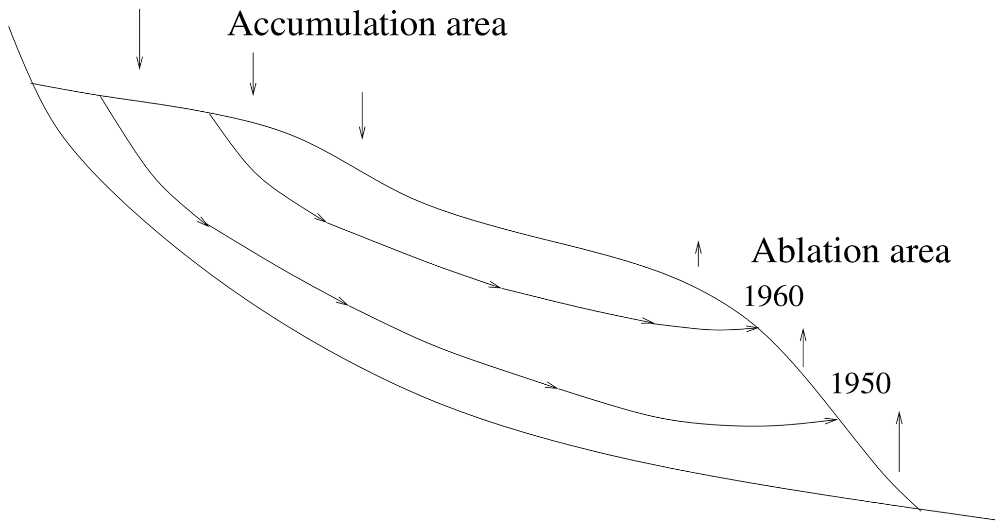
Figure 1 Conceptual representation of ice particles traveling within a glacier ice flow from the accumulation to the ablation area. The oldest ice released is the one that has the longest and slowest trajectories such as the ice found at the glacier snout. Two examples are given based on ice originating from 1960 and 1950.

Existing ice dating methods have been designed mainly for ice cores extracted in accumulation zones with minor ice dynamics to permit the age–depth relationship to be more easily understood. For instance, Eichler et al. (2000) combined multiple methods for dating an ice core extracted at the Grenzgletscher, Switzerland, allowing a yearly accuracy to be achieved. Their methodology includes tracers based on radioactive isotope ²¹⁰Pb (Gäggeler et al., 1983) and seasonally varying signals such as the concentrations of NH${}_{\mathrm{4}}^{+}$ and the isotopic ratio δ¹⁸O, as well as using debris embedded within the ice originating from well-known events such as Saharan dust falls, atmospheric nuclear weapon tests (NWTs) and the reactor accident in Chernobyl (Haeberli et al., 1988). Among them, the NWT fallout related to the 1954–1967 period has been well detected in many ice cores (e.g., Olivier et al., 2004; Gabrieli et al., 2011; Wang et al., 2017) and other archives (e.g., in lake sediments, Röllin et al., 2014) by analyzing the activity of ²³⁹Pu, ²⁴⁰Pu and ²³⁶U radionuclides. No similar dating has been performed at the surface of the ablation area of a glacier, and the question of whether the aforementioned proxies are identifiable after experiencing intense ice deformation and traveling into temperate ice with close proximity to percolation water remains up for debate. To our knowledge, a single unpublished work by Uwe Morgenstern describes the tritium-based dating of surface ice of mountain glaciers. Recently, Gäggeler et al. (2020) used ²¹⁰Pb activity concentration decays of surface ice samples collected in the ablation zone of Aletschgletscher to determine relative ages between samples and deduce ice flow rates. Nevertheless, knowing the absolute age of glacier surface ice would be highly useful for conducting “horizontal ice cores”, i.e., collecting and analyzing old ice (the proxies that have not been altered by ice thermo-mechanical changes) without having to perform expensive and logistically complex deep ice-core drilling (Reeh et al., 2002; Baggenstos et al., 2018). The main challenge when doing so is to find undisturbed isochrones, and to sample across them. Therefore, the efficiency of the method is strongly dependent on our capacity to map the age of the surface ice in order to derive an accurate distance–age relationship – a field of research largely unexplored by ice flow modellers.

In this paper, we combine for the first time ice flow modeling and ice dating based on radionuclide contamination to derive an accurate map of the age of ice at Gauligletscher. (Throughout the entire article, “contamination” refers to a certain concentration level of some key radionuclides in ice samples.) First we use the results of a former model (Compagno et al., 2019) in order to identify the most likely region of the ablation area where ice from the early 1950s and the late 1960s might exist, as this zone is being expected to be contaminated by radioisotopes due to fallout after atmospheric NWT. Then we analyze ²³⁹Pu, ²⁴⁰Pu and ²³⁶U activities from more than 200 ice samples, which have been collected throughout the region identified by the model, to date the ice in a direct way. We take advantage of these new data to refine our ice flow model, to date the entire glacier ice, and to update our prediction of the location of the Dakota airplane (Compagno et al., 2019).

This paper is organized as follows: first, we give a short description of Gauligletscher and the data available to run the model. Then we present the methods for dating the ice based on ice flow modeling and radionuclide contamination. Following that, we present our results and discuss the implications of the new data set for refining the model as well as the implications for the current positions of the wreckage of the Dakota airplane.

2 Study site

Gauligletscher (Fig. 2) is a ≈6 km long glacier covering an area of ≈11 km² located in the Bernese Alps, Switzerland (data from 2010). The glacier has retreated significantly since the start of the monitoring in the 1950s. According to GLAMOS (2018), its tongue lost more than 1 km between 1958 and 2018.

Figure 2 (a) The engine released at the surface of the glacier and found in 2018 (Foto VBS, source: https://www.vtg.admin.ch, last access: 13 November 2020), (b) the Dakota aircraft during the rescue operation in 1946 (Foto MHMLW, source: https://www.vtg.admin.ch, last access: 13 November 2020), (c) aerial view of Gauligletscher taken in summer 2019 (photo: Lars Gnägi). The light and dark shaded areas indicate the low- and high-resolution sampled zones, respectively.

Generally speaking, Gauligletscher has entered our awareness since November 1946, when a Douglas C-53 Dakota airplane crash-landed on its upper accumulation area (Fig. 2). After operations to rescue passengers shortly after and to recover the most valuable pieces in summer 1947, the Dakota main body was left on site, buried gradually under seasonal snow accumulation and transported downstream within the ice flow. Although the plane's pieces were released into the ablation area of the glacier and found between 2012 and 2018, the main body of the Dakota still remains embedded in the ice.

In a previous study, Compagno et al. (2019) modeled the dynamics and the evolution of Gauligletscher and used the model results to reconstruct the space–time trajectory of the airplane to estimate its present position and when and where it will reappear at the surface. The results suggest that the main body of the airplane will be released between approximately 2027 and 2035, 1 km upstream of the parts that emerged between 2012 and 2018. To explain their separation from the main body, Compagno et al. (2019) suggested that the recently found pieces of the Dakota might have been removed from the original airplane location and moved downglacier before being abandoned in 1947.

3 Methods

We now describe in order the methods we used to model the age of ice using both ice flow modeling and radionuclide contamination.

3.1 Glacier model

Prior to sampling, we used the results of Compagno et al. (2019), who modeled the ice flow field and the time evolution of the surface of Gauligletscher from 1947 forward in time, to estimate the region of the glacier where it could be expected that ice from the early 1950s and the late 1960s would be released at the surface. After sampling and data analysis (Sect. 4), we improved the model and performed a range of new model runs, which are presented in this study.

Our model uses the Elmer/Ice finite-element software (Gagliardini et al., 2013) to iteratively compute the ice flow velocity field and the mass balance, and therefore to simulate the time evolution of Gauligletscher, while providing the initial glacier surface digital elevation model (DEM), the bedrock DEM, model parameters and meteorological data. In the next section, we describe the data, the ice flow, the mass balance, the mass transport and the age of ice models. Then we describe our strategy for calibrating the model parameters.

3.1.1 Data

Here we used a wide range of data to run our model, including DEMs from 1947 and 2010, several ground-penetrating radar profiles (Rutishauser et al., 2016) with a resulting bedrock elevation model (Farinotti et al., 2009) (Fig. 3b), recent satellite Sentinel-2 ortho-images to derive a surface ice flow field (Fig. 3a and Appendix A) and meteorological time series of weather stations located nearby. Details concerning the bedrock derivation from radar profiles are given in the Supplementary material of Compagno et al. (2019). For this new study, we also used the 1980 DEM, and an update of observed velocities based on the 2015–2019 Sentinel-2 observations.

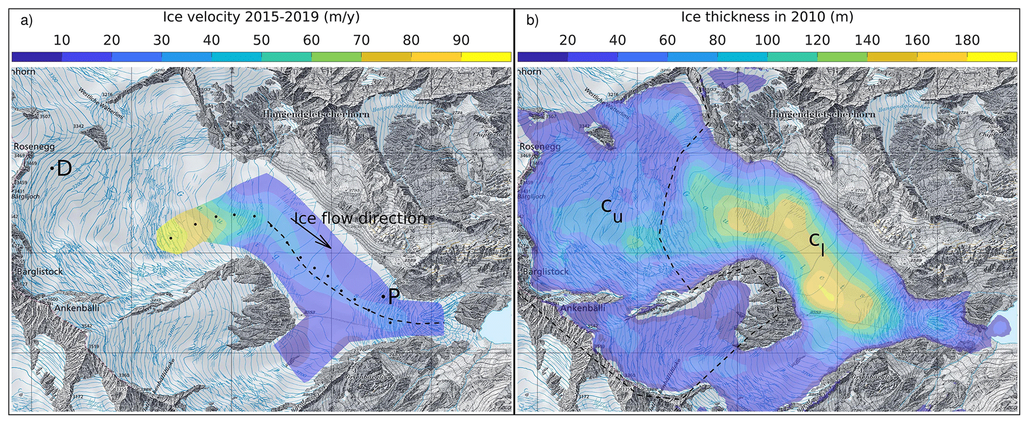
Figure 3 Topographic map of Gauligletscher with 1 km grid spacing showing (a) the observed surface velocities over the period 2015–2019 derived by remote sensing (Appendix A) and (b) ice thickness distribution in 2010. In panel (a), the dashed line shows the line of maximal observed velocities along each lateral transect, while the dots indicate the position where the observed modeled RMSE is computed. The location where the Dakota airplane crash-landed in 1946 and the place where pieces of the plane were released in 2018 at the surface are indicated by the letters “D” and “P”, respectively. In panel (b), the dashed line delimits the lower and upper glacier areas where sliding is parametrized with c_l and c_u, respectively. Reproduced by permission of swisstopo (BA20081).

3.1.2 Ice flow

The motion of ice is described by the full Stokes equations (Greve and Blatter, 2009) based on Glen's law, with Glen's exponent n=3 and constant rate factor A, with ice assumed to be isothermal and temperate. Here we tested values $A=\mathrm{60},\mathrm{100},\mathrm{150}$ MPa⁻³ a⁻¹ to assess the effect of various ice flow regimes from high shearing dominant (high A) to sliding dominant (low A). Note that rate factors A used to model similar Alpine glaciers are usually at the low end of this range, i.e., 60 to 100 MPa⁻³ a⁻¹ (e.g., Gudmundsson, 1999; Jouvet et al., 2011), around the value A=78 MPa⁻³ a⁻¹ recommended for temperate ice by Cuffey and Paterson (2010). As a boundary condition along the bedrock, we used the following non-linear sliding law – known as Weertman's law (Weertman, 1957):

$$\begin{array}{}\text{(1)}& u_{\mathrm{b}}=c{\mathit{\tau }}_{\mathrm{b}}^{\mathrm{1}/m},\end{array}$$

where u_b is the norm of the basal velocity, τ_b is the basal shear stress, $m=\mathrm{1}/\mathrm{3}$ is a constant parameter and c is a sliding coefficient. In our model, c takes two values: c_l and c_u in the lower (“l”) and upper (“u”) parts of the glacier as defined in Fig. 3b, with a smooth transition along a ≈300 m long band between the two zones (not shown). The reason for using two values is that observed surface velocities used to adjust c are available only in the lower part of the glacier, and thus suitable to tune c_l but not c_u. Additionally, the dynamics of the lower part is expected to show more basal sliding (due to an increased presence of meltwater) than those of the upper part, which might even show no basal sliding at all if the ice is frozen to the bedrock (due to lower temperatures in the highest regions). In addition, the upper area is notably shallower than the lower one (Fig. 3b), supporting the choice of a specific tuning parameter for this region. Two regions were therefore defined in order to distinguish the area where surface velocity observations are available (Fig. 3a) and the glacier is thick (Fig. 3b) compared to the rest of the glacier. These two zones defining c_l and c_u roughly correspond to the averaged ablation and accumulation areas over the period 1947–2019, based on an equilibrium line altitude of ≈2900 m a.s.l.

3.1.3 Mass balance

Glacier mass balance (MB) was modeled after integrating the difference between daily solid precipitation P_s (accumulation) and daily melt M (ablation), with correction factors C_P and C_M:

$$\begin{array}{}\text{(2)}& \mathrm{MB}=C_{\mathrm{P}}{P}_{\mathrm{s}}-C_{\mathrm{M}}M.\end{array}$$

On the one hand, daily solid precipitation P_s was equal to precipitation P when daily-average air temperature T is below 0 ^∘C and decreased to zero linearly between 0 and 2 ^∘C. Here the air temperature T and precipitation P were taken from the closest MeteoSwiss weather station and adjusted using linear vertical lapse rates (Huss et al., 2009). On the other hand, daily melt M was computed with a temperature index melt model (Hock, 1999; Huss et al., 2009):

$$\begin{array}{}\text{(3)}& M:=\left\{\begin{array}{ll}\left[f_{\mathrm{M}}+r_{\mathrm{is}}I\right]T& \text{if }T\mathit{>}\mathrm{0},\\ \mathrm{0}& \text{otherwise,}\end{array}\right.\end{array}$$

where $f_{\mathrm{M}}=\mathrm{1.787}\times {\mathrm{10}}^{-\mathrm{3}}$ m d^{−1 ∘}C⁻¹, $r_{\mathrm{i}}=\mathrm{2.146}\times {\mathrm{10}}^{-\mathrm{5}}$ m³ W⁻¹ d^{−1 ∘}C⁻¹ or $r_{\mathrm{s}}=\mathrm{1.608}\times {\mathrm{10}}^{-\mathrm{5}}$ m³ W⁻¹ d^{−1 ∘}C⁻¹ (r_is is r_i or r_s if the surface is covered by ice or snow, respectively) are melt parameters taken from the modeling of Aletschgletscher over the period 1957–1980 (Jouvet et al., 2011), which is located near Gauligletscher, and I(x,j) is the direct solar radiation. In the absence of direct measurements of melt and accumulation, the uncertainty of P_s and M in Eq. (2) might be relatively high. To account for this, we introduced two correction factors C_P and C_M.

3.1.4 Mass transport

For each time step, the ice flow (Sect. 3.1.2) and the mass balance (Sect. 3.1.3) are computed from the current upper surface. In turn, these quantities serve to update the upper surface at the next time step by solving an advection equation often referred to as the kinematic boundary condition (see Eq. (10) in Gagliardini et al., 2013).

3.1.5 Age computation and particle tracking

In addition to ice flow and mass balance equations, we also requested to compute the age of ice a by solving the following transport equation (Gagliardini et al., 2013):

$$\begin{array}{}\text{(4)}& {\displaystyle \frac{\partial a}{\partial t}}+\mathit{u}\cdot \mathrm{\nabla }a=\mathrm{1},\end{array}$$

where u is the modeled velocity field, and t is the time variable. The age of ice takes value 0 as the Dirichlet condition on the inflow boundary. For the sake of simplicity, a was initialized everywhere to zero for the year 1947 as this was sufficient to model the age of the ice formed after 1947. Alternatively, the use of a preliminary stationary model in 1947 could have permitted the modeling of ages to be extended to prior to 1947.

Beside modeling the age of ice, the space–time position of the Dakota airplane and its pieces was inferred by integrating the modeled three-dimensional ice velocity fields by post-processing from their known space positions in 1947 and 2018, similar to Jouvet and Funk (2014) and Compagno et al. (2019).

3.1.6 Model calibration

An ensemble of model runs was performed with different parameters A, c_l, c_u, C_P and C_M. The first three parameters controlled the ice flow strength, while the last two controlled the amount of precipitation and melt (or equivalently the mass balance gradient). Additionally, we assumed that the correction melt factor C_M takes two values $C_{\mathrm{M}}=C_{\mathrm{M},\mathit{<}\mathrm{1980}}$ and $C_{\mathrm{M}}=C_{\mathrm{M},\mathit{>}\mathrm{1980}}$ before and after 1980, respectively, as a DEM was available for the year 1980. We selected three values $A=\mathrm{60},\mathrm{100},\mathrm{150}$ MPa⁻³ a⁻¹ and four values $C_{\mathrm{P}}=\mathrm{1},\mathrm{1.2},\mathrm{1.35},\mathrm{1.5}$ that were chosen in a physical range. For each pair of parameters (A, C_P) among the 12 possible combinations, the procedure to calibrate the three remaining ones (c_l, c_u, and C_M) consisted of several steps (summarized in Fig. 4) which were repeated until the convergence was reached:

• i.

  The sliding parameter in the lower part c_l was found to minimize the root mean square error (RMSE) between the modeled and observed velocities along 14 points located along the central flowline (Fig. 3a) during the period 2015–2019 after modeling the 2010–2019 period, starting from the most recently available DEM (2010). The choice of considering only 14 points distributed along the central flowline was made to reduce underfitting in the minimization procedure, which optimizes a single parameter.

• ii.

  Parameter C_M,<1980 was found to minimize the RMSE between modeled and observed DEMs in 1980 after modeling the period 1947 to 1980.

• iii.

  Parameter C_M,>1980 was found to minimize the RMSE between modeled and observed DEMs in 2010 after modeling the period 1980 to 2010.

• iv.

  The sliding parameter in the upper part c_u is calibrated to get the best match between modeled and “observed” age of ice, where ice from 1960 was identified along line 3 (see Fig. 6 and Sect. 4.2). In the optimization loop, c_u is kept in the range [1,50] km MPa⁻³ a⁻¹, which extends from nearly no sliding (c_u=1) to high basal motion (c_u=50).

Note that only 2 to 3 loops over the steps were necessary to achieve convergence of the parameter set. After calibration, we obtained 12 parameter sets (Fig. 4), which resulted from $A=\mathrm{60},\mathrm{100},\mathrm{150}$ MPa⁻³ a⁻¹ and $C_{\mathrm{P}}=\mathrm{1},\mathrm{1.2},\mathrm{1.35},\mathrm{1.5}$. While the calibration model runs used a 100 m resolution mesh to allow sequential multiple runs to be performed, we recomputed the 12 model runs with optimal parameter sets at a finer resolution (50 m) for further analysis.

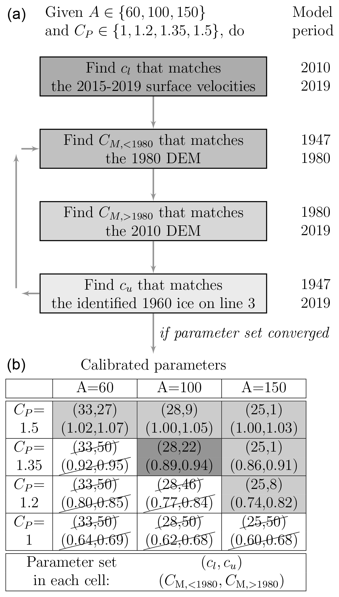
Figure 4 Calibration scheme (a) used in this study to find optimal parameters c_l, c_u, C_M,<1980 and C_M,>1980, for given A and C_P parameters, and parameter sets obtained after calibration (b). In practice, a very few iteration loops over the steps were sufficient to achieve convergence. The grey cells correspond to the parameter sets that were kept for analysis – the strike-through ones being discarded for yielding unrealistic results (Sect. 4.3). The dark grey cell indicates the closest to the mean of the six retained parameters and was taken as the best-guess parameter set.

3.2 Radionuclide sampling and analysis

Here we make use of some isotopes trapped in ice samples to find out the source and the time of contamination. From previous studies (e.g., Olivier et al., 2004; Gabrieli et al., 2011; Wang et al., 2017), the highest isotope concentrations of ²³⁹Pu from NWTs (up to several mBq kg⁻¹) are expected in the ice from 1962 to 1963, with a rapid decrease afterwards. On the other hand, ²⁴⁰Pu and ²³⁶U concentrations are expected to be of the same order of magnitude with isotope ratios ²⁴⁰Pu∕²³⁹Pu and ²³⁶U∕²³⁹Pu of ≈0.2 and ≈0.3 for global fallout. In this section, we describe the sampling collection and the concentration analysis with mass spectrometry, which includes the separation of uranium (U) and plutonium (Pu).

3.2.1 Sample collection

In summer 2019, more than 200 surface samples were collected along five lines at the ablation zone of Gauligletscher (Fig. 5). Note that in summer 2018, 80 samples were collected as well, albeit along a single central line (Fig. 5). Sampling lines were chosen to roughly follow flowlines whenever possible. Deviations from the planned sampling lines were allowed in the field in order to avoid crevasses. In summer 2019, the sampling area was determined to cover the 1954–1967 isochronal band derived from the original model by Compagno et al. (2019), with a high-resolution sampling zone (every ≈25 m) in the region designated by the model, and a low-resolution sampling zone (every ≈50 m) further downstream and upstream for safety reasons.

Figure 5 Topographic map of Gauligletscher with 1 km grid spacing showing the 1954, 1960 and 1967 isochrones inferred from the original (yellow contour lines) and the revised best-guess (magenta contour lines) models, the five sampling lines (defined by “L1” to “L5”, and indicated by black dots), and the contaminated locations (where ²³⁹Pu activities exceed 0.25 mBq kg⁻¹) depicted by red dots, whose size corresponds with the ²³⁹Pu activity. The squares and circles show the locations along each line identified as originating from 1960 and 1963 in Fig. 6, respectively. Crosses indicate measurement outliers not included for analysis. The shaded area corresponds to the region sampled in high resolution (i.e., ≈25 m rather than ≈50 m). The dashed line shows the line of maximal observed velocities along each lateral transect. The blue circles mark the line sampled in 2018, where no ²³⁹Pu activities >0.1 mBq kg⁻¹ have been found. Reproduced by permission of swisstopo (BA20081).

At each location, the sample ground was chosen to be located on visually dry ice at least 2 m away from surface meltwater flow. The topmost layer (≈30 cm) of ice was cleared, and then a minimum of 2 L of dry crushed ice was removed from the glacier by means of a drill (8 cm, 1 m long). The samples were collected under sunny weather conditions, and mainly in the morning with a minimum amount of meltwater flow on the glacier surface. The ice was left to melt for 2 d in the polypropylene sample container, which resulted in 1.2 L water. The GPS coordinates of all sampling locations were recorded.

3.2.2 Measurements

Uranium (U) and plutonium (Pu) were separated prior to any measurement activities. Details of the sample preparation is described in Appendix C. The mass spectrometry (MS) analysis of Pu and U was carried out at Spiez Laboratory using a multicollector inductively coupled plasma mass spectrometer (Neptune, Thermo Fisher). A self-aspirating PFA-ST nebulizer and a SC-2DX autosampler (Elemental Scientific Incorporation) were used to introduce the samples. All MS measurements were conducted in low-resolution mode (R=300).

For Pu measurements, a desolvating system (Aridus II, CETAC Technologies) was used to enhance the signal and to achieve low hydride and oxide formation. In this configuration, the sensitivity for U was about 1  ×  10⁸ counts per second (cps) per ng mL^{−1 238}U. All Pu isotopes were measured by secondary electron multiplier (SEM) detectors. In order to correct for U and thorium (Th) interferences due to hydride generation and tailing, 10 ng mL⁻¹ U and Th standard solution were measured using Faraday detectors. Typical correction factors for the m∕z 239, 240 were 3  ×  10⁻⁶, 5  ×  10⁻⁷ for ²³⁸U and 4 × 10⁻⁸, 8 × 10⁻⁹ for ²³²Th. Pu isotope concentrations were calculated from the signal of the ²⁴²Pu tracer. The contributions of the Pu isotopes from the tracer were corrected mathematically based on the isotope ratios from the certificate. Considering the variations of these effects, the detection limit was estimated to be 2 × 10⁻³ mBq kg^{−1 239}Pu. The total acquisition time per sample was 3 min.

For U isotope ratio measurements, a Twinnabar (Glass Expansion) spray chamber was used. The sensitivity for U was about 6 × 10⁶ cps per ng mL^{−1 238}U. ²³⁵U and ²³⁸U were measured by means of Faraday detectors and the minor isotopes by SEM detectors. For the measurement of ²³⁶U, a retarding potential quadrupole filter was used to lower the abundance sensitivity. The U and Th tailing was corrected using a baseline subtraction. Hydride interference was corrected mathematically. Considering these effects, the detection limit was estimated to be 3 × 10⁻⁵ mBq kg⁻¹ U²³⁶. Standard sample bracketing using the IRMM-187 U isotope standard was applied for all measurements. IRMM-184 isotope standard was used for quality assurance. The total acquisition time per sample was 18 min.

4 Results

4.1 Original model results

The original model from Compagno et al. (2019) was used to predict the most likely place on Gauligletscher where ice from 1954 to 1967 might appear – the period with the highest inputs of ²³⁹Pu in an ice core at Colle Gnifetti glacier, Switzerland (Gabrieli et al., 2011). As a result, the model yields an asymmetrical U-shaped isochronal band located about 1 km above the current glacier tongue (Fig. 5), which served to delineate the glacier region to be sampled (Sect. 3.2).

4.2 Dating with radionuclides

Figures 5 and 6 show the ²³⁹Pu and ²³⁶U activities of the samples in plain view and along the five sampled lines, respectively. The two tracers were found to be consistent in terms of pattern, and at the same time to indicate contaminated regions (above 0.25 mBq kg⁻¹ in ²³⁹Pu; see Fig. 6). By contrast all the samples collected in summer 2018 show very small activities (below 0.1 mBq kg⁻¹ in ²³⁹Pu, results not shown) since the ice sampled in 2018 was mostly likely too young to be contaminated (Fig. 5). Therefore, only 2019 sampling results were considered in the following.

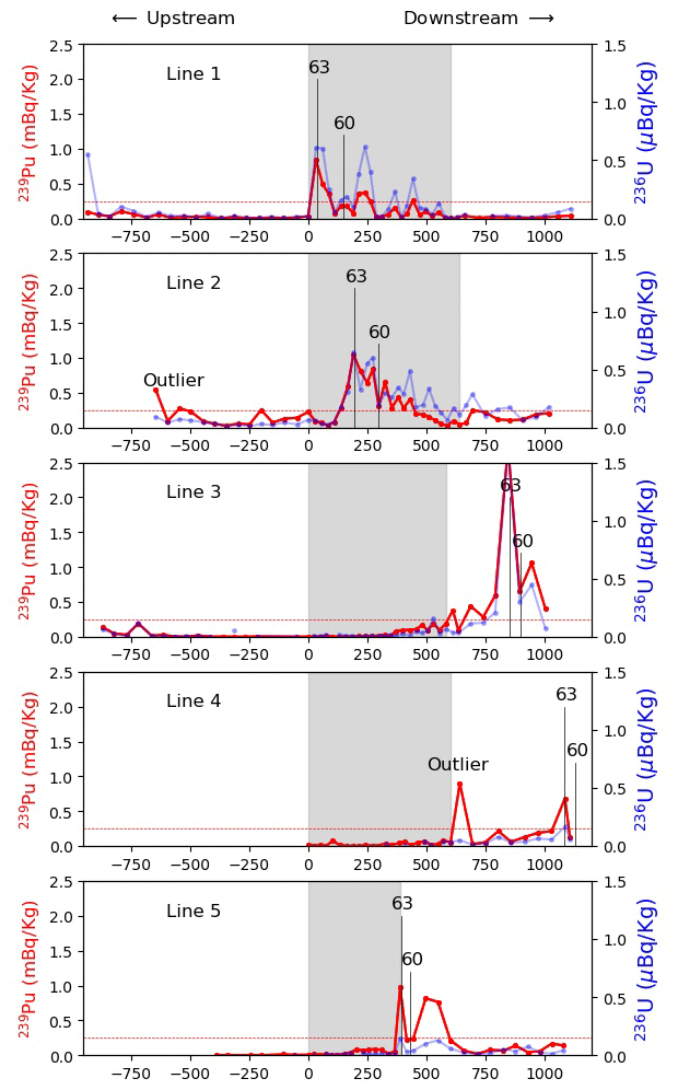
Figure 6 Activities of ²³⁹Pu and ²³⁶U along the five sampled lines as defined in Fig. 5 from upstream to downstream. The shaded area correspond to the region sampled in high resolution (i.e., ≈25 m instead of ≈50 m). The vertical line depicts the position where ice from 1960 and 1963 have been identified (±2 or ±6.5 years). The threshold 0.25 mBq kg⁻¹ used to qualify contaminated samples in Fig. 5 is indicated by a dashed horizontal line. Note that the uncertainty associated with ²³⁹Pu measurement is less than 4 % for all samples that are above 0.1 mBq kg⁻¹.

Unfortunately, the contaminated region was captured only in the high-resolution sampling zone for lines 1 and 2 and is part of the low-resolution surrounding zone for other lines (Figs. 5 and 6). Following the footprint of ²³⁹Pu in the ice cores at Colle Gnifetti (Gabrieli et al., 2011), Switzerland, and the eastern Tian Shan (Wang et al., 2017), Central Asia, the contaminated region was expected to correspond to the 1954–1967 period, which roughly extended from the first atmospheric NWT (≈1953) to the last ones (≈1963) when the USA and the USSR signed the Limited Test Ban Treaty (Fig. 1, Gabrieli et al., 2011). The highest ²³⁹Pu activity (found on line 2) shows ≈2.5 mBq kg⁻¹, which is about 2–3 times less than the highest ones found in the ice cores at Colle Gnifetti (7 mBq kg⁻¹), and the eastern Tian Shan (5.5 mBq kg⁻¹); however, it is slightly above the highest activity (2.165 mBq kg⁻¹) measured in an ice core extracted from the Dome du Gouter, Mont Blanc, France (Table 7, Warneke et al., 2002).

Activities of ²⁴⁰Pu (not shown) follow a pattern very similar to the ²³⁹Pu ones, with a ²⁴⁰Pu∕²³⁹Pu ratio close to 0.2, which is a well-known value representing average fallout from US and USSR NWTs (Krey et al., 1976). Note, however, that this only concerns samples with ²³⁹Pu activities above 0.25 mBq kg⁻¹ as the ²⁴⁰Pu signal was disturbed by unknown interferences for some samples with low ²³⁹Pu activities. We observe that ²³⁶U activities also follow a pattern similar to ²³⁹Pu (Fig. 6). Furthermore, the peak activity of ²³⁶U in line 3 (≈1.6 µBq kg⁻¹) is comparable with the one found in the ice core at the eastern Tian Shan glacier (≈1.5 µBq kg⁻¹), which is given in Table 2 of Wang et al. (2017). Nevertheless it must be stressed that interferences on the ²³⁶U signal caused the mass ratio of ²³⁶U∕²³⁹Pu to vary between 0.2 and 3. Therefore ²³⁶U was not further considered for dating purposes.

The contaminated band clearly shows a double-peak structure for lines 1 and 5, a less pronounced one for line 3, multiple peaks for line 2, and a single dominant peak for line 4 (Fig. 6), after discarding the first one (see next paragraph). These two peaks are characteristic of the periods 1954–1958 and 1962–1963, respectively, matching the chronological order of NWT activities worldwide (Carter and Moghissi, 1977; Gabrieli et al., 2011; Wang et al., 2017). The first period spans more than ≈5 years and ends with a maximum in 1958, while the second period is shorter but more intense, with a maximum in 1963. We made use of this double-peak structure to identify ice from 1963 – the highest and most recent peak – and ice from 1960 – the midway year between the two peaks characterized by a local minimum. The ice in 1963 is found at the highest and most upstream ²³⁹Pu activity location. It was easy to identify 1963 ice on all lines (Fig. 6) after filtering out a few outliers (see next paragraph). The locations of the ice from 1963 are associated with a ±2-year uncertainty, which corresponds to the width of the peak. On the other hand, 1960 ice was easily found between the two detected peaks of lines 1, 3 and 5. We also associate it with a ±2-year uncertainty, which corresponds to the distance between the two peaks. By contrast, the interpretation was more difficult for lines 2 and 4. Line 2 shows 3 peaks above 0.25 mBq kg⁻¹, which might be caused by the near alignment of the sampling line with the isochrone (Fig. 5). We chose midway between the two highest peaks in ²³⁹Pu but increased the uncertainty to ±6.5 years, which corresponds to the length of the 1954–1967 period. By contrast, the high end of line 4 coincides with the highest observed velocities (Fig. 3), indicating that the 1960 position sought along this line is expected to be the most downstream one of all five lines. This statement is supported by subsequent modeling results (Fig. 5). By comparing the ²³⁹Pu activities found on lines 3 and 4, we find a similar pattern for the presumed 1962–1963 peak (Fig. 6), the other peak associated with 1954–1958 likely being missed due to its location further downstream from the sampled area. We therefore inferred the 1960 position along line 4 by analogy with the one found on line 3 (Fig. 6).

Let us note that four samples with ²³⁹Pu activities above ≈0.25 mBq kg⁻¹ were found away from any identified contaminated areas (see “outliers” in Figs. 5 and 6). Two of these outliers (on line 2) have activities just above the threshold value. This justifies their disqualification. However, there remain two isolated outliers on lines 2 and 4 with activities of ≈0.5 and ≈1 mBq kg⁻¹, respectively, which might be caused by sampling or measurement errors. Note that the unexpected isolated high activity seen on line 4 might be due to the alignment of the sampling line with the isochrone.

4.3 Revised model results

Figure 5 shows that the 1960 and 1963 ice revealed by radionuclide contamination is quite far downstream of the ice predicted by the original model (Compagno et al., 2019). To investigate this, we explored further ice flow (A, c_l, c_u) and mass balance (C_P and C_M) parameters on the basis of 12 new model runs (Fig. 4b).

For each A, parameter c_l was found to match observed surface velocities of the ablation area over the 2015–2019 period (Figs. 3a and 7c). As a result, the inferred parameters led to higher c_l (i.e., higher sliding velocities) as compared to parameter $c_{\mathrm{l}}=c_{\mathrm{u}}=\mathrm{12.5}$ km MPa⁻³ a⁻¹ of the original model by Compagno et al. (2019) with A=60 MPa⁻³ a⁻¹. This is due to the new data set of observed velocities (Appendix A), which showed faster ice in the ablation area than the data set used formerly. On the other hand, C_M,<1980 and C_M,>1980 were found to match observed DEMs in 1980 and 2010 for all parameters $A\in \mathit{\{}\mathrm{60},\mathrm{100},\mathrm{150}\mathit{\}}$ and $C_{\mathrm{P}}\in \mathit{\{}\mathrm{1},\mathrm{1.20},\mathrm{1.35},\mathrm{1.5}\mathit{\}}$ (Fig. 7). This is a major difference with our former model (Compagno et al., 2019), which used only C_P=1. Thus we explored a stronger mass balance vertical gradient, i.e., higher precipitation and higher melt amplitudes, as no direct measurements were available there. Lastly, in the absence of direct ice flow measurements in the accumulation area, we adjusted the sliding parameter there (c_u) to match the age of ice identified by radionuclide contamination.

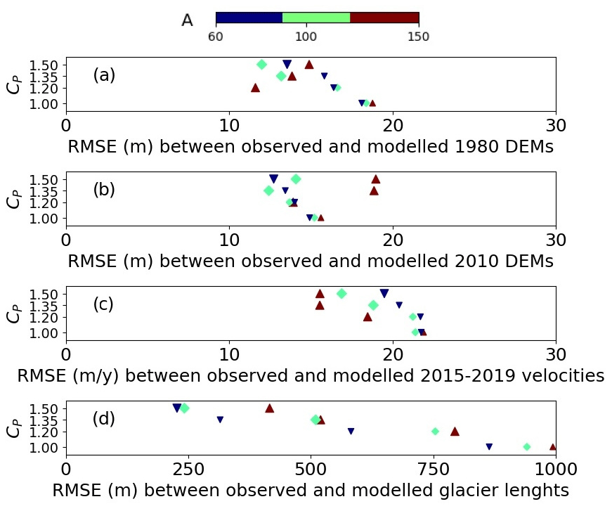
Figure 7 Root mean square error (RMSE) between modeled and observed variables for the 12 model runs (indexed by C_P and A) relating to the 1980 DEM (a), the 2010 DEM (b), the 2015–2019 surface velocities (c) and the length of the glacier tongue (d). Large (or small) symbols indicate the parameter sets that yield realistic (or unrealistic) results and then were kept (or discarded) for analysis (Fig. 4).

As a result of this calibration, 6 of the 12 model runs (see shaded cells in Fig. 4) provided results which were far more realistic mainly with C_P=1.35 and C_P=1.5, i.e., with 35 %–50 % more precipitation correction than the ones obtained using C_P=1:

• i.

  All model runs except one based on the two lowest C_P values led to higher sliding in the upper zone (c_u) than in the lower zone (c_l), which was an unrealistic situation, as sliding was expected to increase at lower elevations (due to the presence of further meltwater and temperate ice).

• ii.

  The value of $C_{\mathrm{P}}=\mathrm{1.35},\mathrm{1.5}$ always led to a substantially improved agreement between observed and modeled glacier length evolution (Fig. 7d).

• iii.

  To a lesser extent, $C_{\mathrm{P}}=\mathrm{1.35},\mathrm{1.5}$ led to a better match between observations and modeling in terms of DEMs and 2015–2019 surface velocities (Figs. 7a, b, and d).

Based on these findings, we discarded six model runs that yielded unrealistic situations (strike-through cells in Fig. 4) and kept only the six remaining ones for further analysis (shaded cells in Fig. 4).

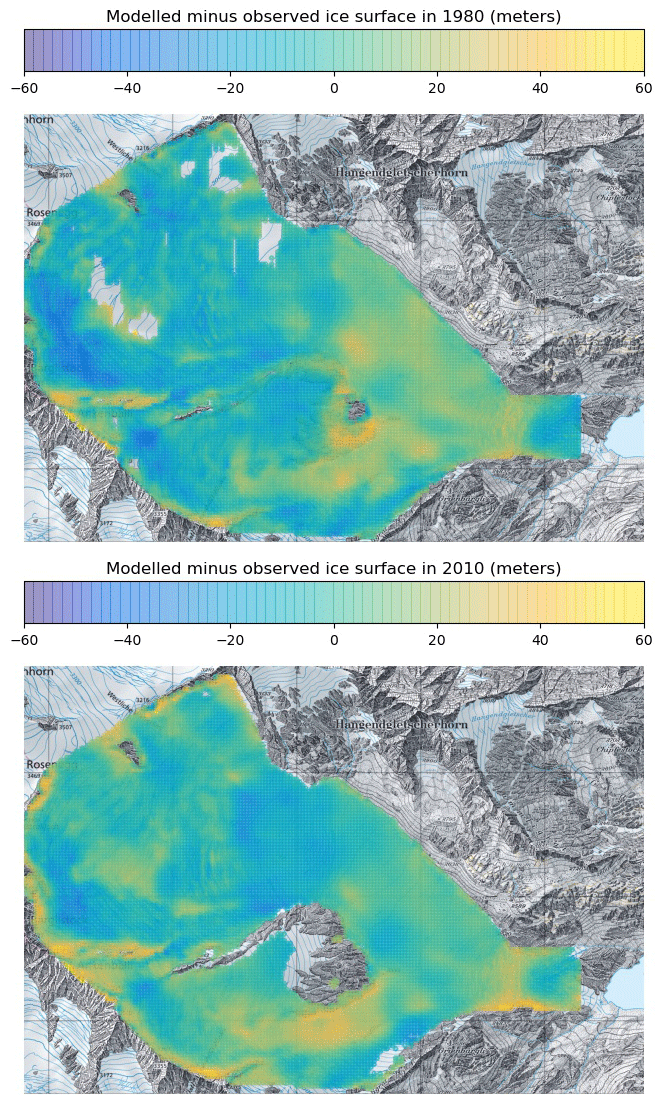
Interestingly, the parameter set that was the closest to the mean of the six retained sets showed values of A=100 MPa⁻³ a⁻¹, ($c_{\mathrm{l}},c_{\mathrm{u}})=(\mathrm{28},\mathrm{22})$ km MPa⁻³ a⁻¹, C_P=1.35, $C_{\mathrm{M},\mathit{<}\mathrm{1980}}=\mathrm{0.89}$ and $C_{\mathrm{M},\mathit{>}\mathrm{1980}}=\mathrm{0.94}$ (Fig. 4), which were very similar to the values calibrated for Aletschgletscher in another study (Jouvet et al., 2011) – namely A=100 MPa⁻³ a⁻¹, $(c_{\mathrm{l}},c_{\mathrm{u}})=(\mathrm{23.3},\mathrm{0})$ km MPa⁻³ a⁻¹, C_P=1.35 and C_M=1. Note that unlike Gauligletscher, the mass balance parameters calibrated for Aletschgletscher were based on direct measurements of melt and accumulation. We therefore selected this parameter combination as our best guess set. Figure B1 in Appendix B compares modeled and observed ice surface elevations 33 and 63 years after the model initialization obtained with the best guess model. Although the error pattern is quite heterogeneous, it is fairly balanced between the ablation and accumulation areas.

Figure 8 shows the modeled age of ice at the location where ice was identified as originating from 1960 and 1963. As a result, we get a much better agreement between modeled and observed 1960 and 1963 age at lines 3 and 4 when comparing new to former model results. Note that this was expected for line 4 as the model was adjusted to give the best agreement for 1960. Focusing on line 3, which has the narrowest interval of confidence, the six model runs revealed a very good fit. Figure 5 displays the 1960 isochrone in plain view, obtained using the original and the revised best-guess models, respectively, and confirms the substantial improvement achieved for matching radionuclide-based dated ice. In contrast, a relatively high mismatch between observation and modeling was found for side lines 1 and 5. Indeed, modeled age at the 1960 and 1963 identified positions on line 1 was largely overestimated (by more than a decade), while the one for line 5 was underestimated by the same amount (Fig. 8). Figure 5 illustrates the model–observation mismatch in terms of isochrones: the model tends to exaggerate the asymmetry in the ice flow (visible in Fig. 3), resulting in ice that is too slow (i.e., too old) in the north-east side and ice that is too fast (i.e., too young) on the south-west side. As the flow asymmetry was directly controlled by the bedrock topography (Fig. 3b) or sliding basal conditions, it is likely that this mismatch can be corrected by adjusting the bedrock lateral profile, i.e., making it deeper where ice is found to be too old and slow, and vice versa, or by allowing the sliding coefficient c_l to vary laterally to obtain the same result. To a lesser extent, the discrepancy between the modeled and observed age of ice on line 2 can be explained in a similar way.

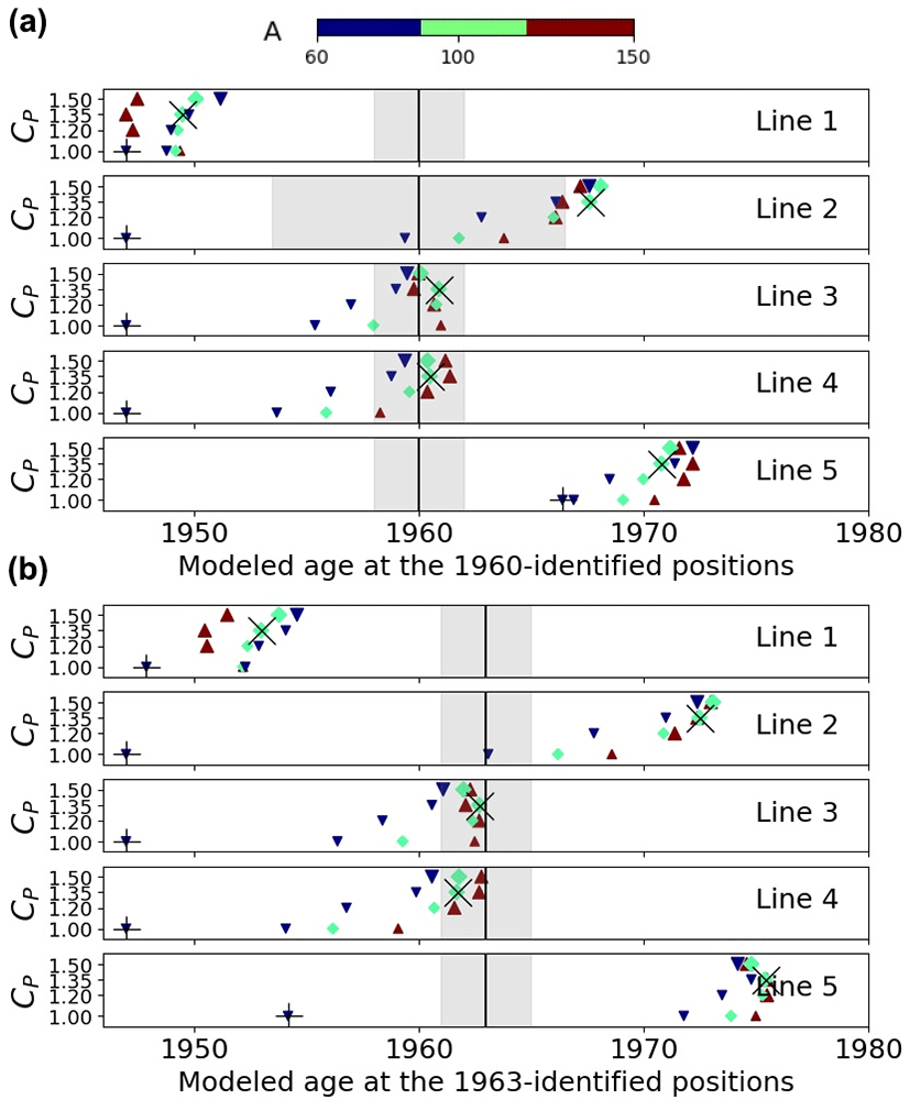
Figure 8 Modeled age of ice at the location where ice has been identified as originating from 1960 (a) and 1963 (b) in Fig. 6 for the 12 new model runs. The grey area represents the interval of confidence. Symbols + and × designate the results of the original model by Compagno et al. (2019) and the best-guess model run among the 12 (Fig. 4), respectively. Large (or small) symbols indicate the parameter sets that yielded realistic (or unrealistic) results and then were kept (or discarded) for analysis.

Thanks to the newly calibrated model, we could derive the age of ice everywhere at the surface of Gauligletscher (Fig. 9). The results show that most of the current ablation zone released ice prior to 1950. Note that our map is incomplete as we did not model ice older than 1947 – the year of initialization. Interestingly, the most recent modeled isochrones (after 1970) are U-shaped while the much older ones (before 1970) are V-shaped. Here we can reasonably assume that the downstream tightening of isochrones follows the narrowing of the channel, which hosts the glacier tongue. The peaks of the U and V roughly coincide with the maximal velocity across glacier lateral transects (Fig. 9). The asymmetry between the left and right lateral margins was quite strong, and probably stronger than it is in reality due to an inaccurate bedrock or basal sliding parametrization as discussed before.

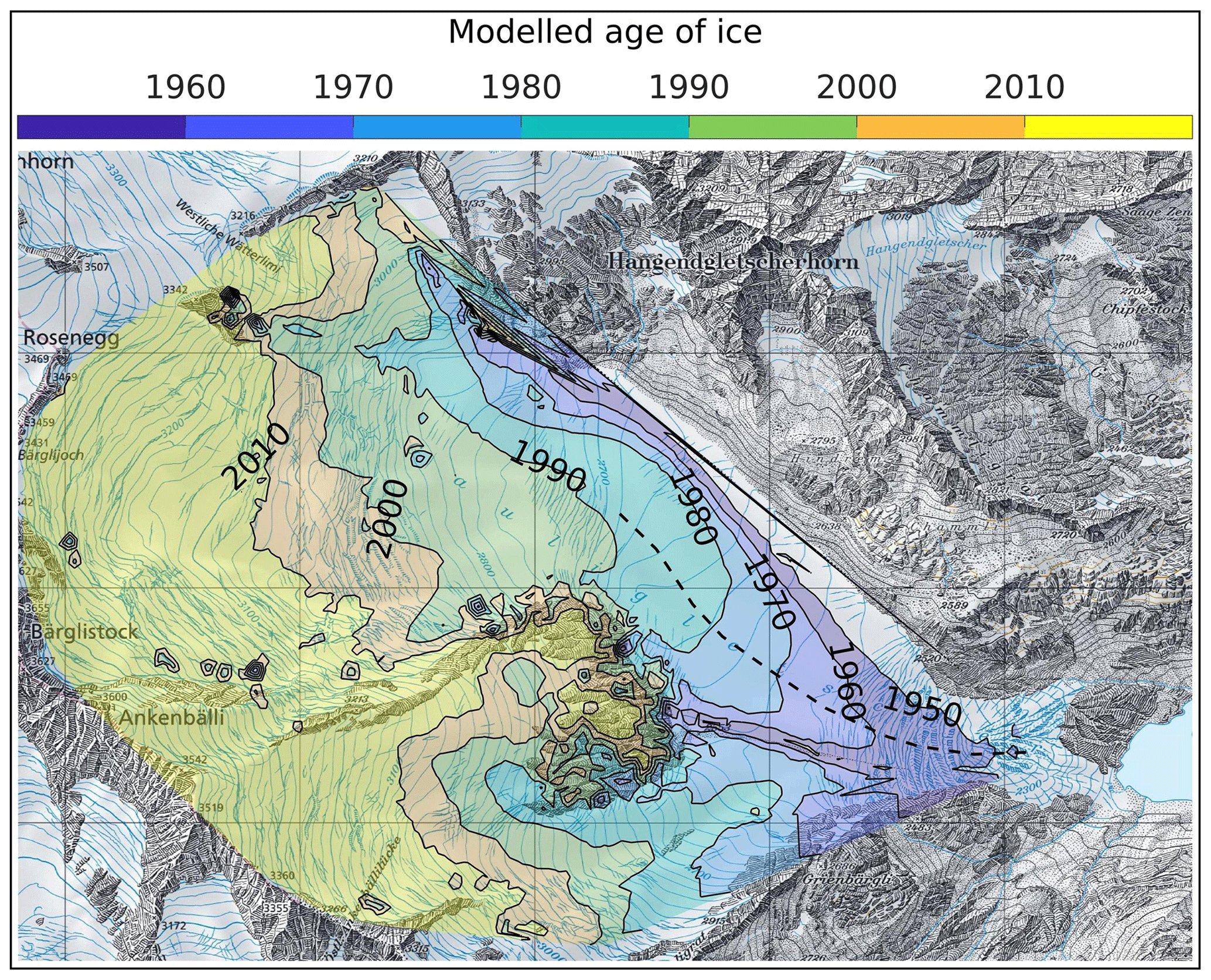
Figure 9 Topographic map of Gauligletscher with 1 km grid spacing showing the modeled age of ice at the surface using the best-guess model run (Fig. 4). The dashed line shows the line of maximal observed velocities along each lateral transect. Reproduced by permission of swisstopo (BA20081).

5 Discussion

The results of the sampling campaign demonstrate that the region featuring higher ²³⁹Pu, ²⁴⁰Pu and ²³⁶U activities coincides with the area where ice originates from the early 1950s to the late 1960s:

• Contamination in both radionuclides has the same pattern and for the most part appears band-wise (Fig. 5). The sampled lines show ≈300 m long bands with ²³⁹Pu activities mostly above 0.25 mBq kg⁻¹ (Fig. 6) up to 2.5 mBq kg⁻¹, which is in line with the highest activities found in three different ice cores (≈2.2, 5.5 and 7 mBq kg⁻¹). These contaminated bands presumably reflect the most intense period in terms of NWT, namely 1954–1967 (Gabrieli et al., 2011). As this period lasted roughly 13 years, this corresponds to a mean ice flow of ≈23 m yr⁻¹, which is in the high end of the 2015–2018 ice flow observations along those lines (13–22 m yr⁻¹; see Fig. 3); however, as the ice was thicker in the past it most likely exhibited faster flow as well. By contrast, off-band samples show very low activities (under 0.1 mBq kg⁻¹) with few exceptions (Fig. 6). Note that the exact peak activity year (1958 or 1963) might have been missed as the sampling distance (≈25–50 m) corresponds to a ≈1–3-year time interval.

• The contaminated part of line 2 is located slightly above the location where pieces from the Dakota airplane were found in 2018 (Fig. 3a). Regardless of the location where the pieces were absorbed by the glacier, the ones released in 2018 are located on an isochrone associated with the year 1947, i.e., 5 years before the period where contamination should be observed. The position of the contaminated band and of the released pieces is therefore consistent, since the surface ice is expected to be older downstream than upstream (Fig. 1).

• Three lines (1, 2 and 5) show a double-peak structure in ²³⁹Pu, ²⁴⁰Pu and ²³⁶U activities, which are typical of the years 1957 and 1963 (Wang et al., 2017). The spacing between the two peaks (100–150 m, Fig. 6) is again consistent with an ice flow speed of ≈20 m yr⁻¹ and the 5–7-year interval. The double peaks of lines 3 and 4 were missed most likely because of insufficient sampling resolution and a sampling area that is too small (the presence of large crevasses prevented us from sampling further downstream).

• The shape of the contaminated bands is consistent with the observed ice flow (Fig. 3a): the contaminated bands of central flowlines are shifted downstream compared to the lateral flowlines and the lowermost one is located on the profile where observed velocities are maximal.

• The ²⁴⁰Pu∕²³⁹Pu ratio was found to be close to 0.2 for the most part, which is a well-known value representing average fallout from the US and USSR NWT (Krey et al., 1976).

• Another line located upstream of the contaminated region was sampled and analyzed in summer 2018 (results not shown). No ²³⁹Pu activity above 0.1 mBq kg⁻¹ was detected, similar to the upper part of line 3 in 2019, which is located nearby. Corroborating the 2018 and 2019 sampling supports the fact that the radionuclide contamination is stable in space and time.

Based on this evidence, we identified ice from 1960 and 1963 with an accuracy of a few years. To our knowledge, this is the first time that plutonium-based tracers have been used to date ice in the ablation zone of an Alpine glacier.

Our original model (Compagno et al., 2019) predicted ice from 1954–1967 located mostly upstream of the ice revealed by ²³⁹Pu, ²⁴⁰Pu and ²³⁶U contamination (Fig. 5). To correct the model, we enlarged the parameter space to test further ice flow and mass balance regimes and recalibrated our model accordingly (Fig. 4). The newly calibrated model permits a significantly better agreement to be achieved between the modeled and the radionuclide-based 1960 and 1963 ice (Fig. 8). The new data can even serve to further constrain our parameter space: the six model runs based on low precipitation rates delivered unrealistic situations and then were discarded. As a result of the recalibration, we found that ice flow, precipitation and melt were underestimated in our original model. Interestingly, the best-guess parameter set is very similar to the optimal parameter set found for modeling Aletschgletscher from 1880 to 1999 (Jouvet et al., 2011), all of these parameters being calibrated against measurements and validated by means of an independent tracer (Jouvet and Funk, 2014).

The sparsity of data used for tuning the ice flow model is a well-known source of model uncertainty. Indeed, observed surface velocities used to adjust key parameters only cover restricted areas and time frames (i.e., mostly the ablation area for the recent past) due to limitations in remote sensing methods. Indeed, snow-covered accumulation areas show hardly any features that can be tracked, and there is hardly any usable satellite data prior to the 1990s. Thus our model might poorly reproduce the ice flow in the distant past and/or over the accumulation area. Furthermore, several ice flow and mass balance regimes (from slow ice and low mass balance gradient to fast ice and high mass balance gradient) can reproduce observed DEMs in a similar fashion – an ambiguity that sparse data cannot resolve. By contrast, tracers such as radionuclides yield much more global data (in space and time) as they result from the long-term glacier movement and mass balance. Tracers further reflect the ice dynamics over the entire glacier thickness – the surface isochrones being different if ice particles have deep or shallow trajectories. From a modeling perspective, such datable tracers (or more generally Lagrangian data) are therefore extremely valuable, as they potentially can constrain the space of model parameters much better than a modern data set of observed ice velocities can do. Here, radionuclide-based data also permitted precipitation and melt upwards in the mass balance models to be substantially revaluated.

Our results also shed light on the influence of the bedrock topography and basal conditions on isochrones. Here, the bedrock was inferred by interpolating ice thickness profiles obtained by ground-penetrating radar (GPR) (Rutishauser et al., 2016). Therefore, the bedrock data might be locally inaccurate if the reflectance is not well interpreted or due to interpolation errors; see the supplementary material of Compagno et al. (2019) for details on the bedrock derivation. Here our bedrock data might be too shallow on the north-east side and too deep on the other side to explain the mismatch between modeled and observed isochrones. Therefore, surface isochrones such as the ones revealed here by plutonium contamination can be used to optimize the bedrock, in particular by correcting its shape along lateral glacier sections. In a similar fashion, these data can serve to optimize the parametrization of basal sliding, which was kept simple in this study (piece-wise constant with only two parameters). While surface observed ice flow velocity are data commonly used to interpolate GPR-based measured profiles, and to derive entire bedrock elevation distribution (e.g., Morlighem et al., 2011) or spatially variable basal parametrizations (e.g., Gagliardini et al., 2013) by inverse modeling, the use of Lagrangian data could provide new insights and should be investigated further.

Here we investigated anthropogenic ²³⁹Pu, ²⁴⁰Pu and ²³⁶U contamination in order to discover isochrones of relevance for the release of ice in the ablation zone of a temperate Alpine glacier. It is important to note that other tracers might be worth considering as well. Using atmospheric NWT related to the 1954–1967 period is suitable for dynamic Alpine glaciers for several reasons. First, the typical timescale for the transportation of ice particles from the top to the bottom varies from a few decades to a few centuries (according to the glacier size and dynamics) and the most relevant period (1954–1967) is ≈60 years old. Second, this period extends over more than a decade with a typical double-peak structure, which makes it easily detectable. Last, in general climate conditions during the 1954–1967 period were characterized by significant net accumulation layers (in contrast with post-1980s) favoring the preservation of the signal left by the fallout of atmospheric NWT. By contrast, sporadic events such as the nuclear accident at Chernobyl (Haeberli et al., 1988), Saharan dustfalls (Wagenbach and Geis, 1989) and volcanic events (Kellerhals et al., 2010), which have been detected in ice cores located in accumulation zones, might be too short-lived to be detected at the surface of the ablation area. The main challenge for finding alternative tracers is to locate some that have not been washed away by percolating meltwater in the ablation area. Here we found that the ²³⁹Pu signal at the surface of Gauligletscher is very close to the activity found within an ice core extracted near Mont Blanc (Warneke et al., 2002), and about 3 times less than the activity found within an ice core extracted at Colle Gnifetti (Gabrieli et al., 2011).

6 Implications for the Dakota

Using an early version of the model (Compagno et al., 2019), we estimated both the current position and the future emergence of the Dakota airplane, which crash-landed on Gauligletscher in 1946 and was subsequently buried within the ice (Sect. 2). Our new model calibrated with radioisotope data permits a significant update of this estimate. According to our best-guess model run (Fig. 4), the Dakota would have reached a maximum depth of 120 m under the surface in the late 1980s and would have emerged at the surface around 2015 slightly downstream from the place where pieces were found between 2012 and 2018 (Fig. 10a). This indicates that the main body of the Dakota most likely lies in this region close to the ice surface and will emerge there in the coming years. This new model result is in stark contrast to our previous one, which estimated a trajectory of roughly half this length (Fig. 10a) and half this depth (the maximal depth computed by Compagno et al., 2019, was 68 m). This illustrates the significant underestimation of ice fluxes in the former model and demonstrates the great added value of the newly used Lagrangian data to refine our modeling of the mass balance and the ice flow.

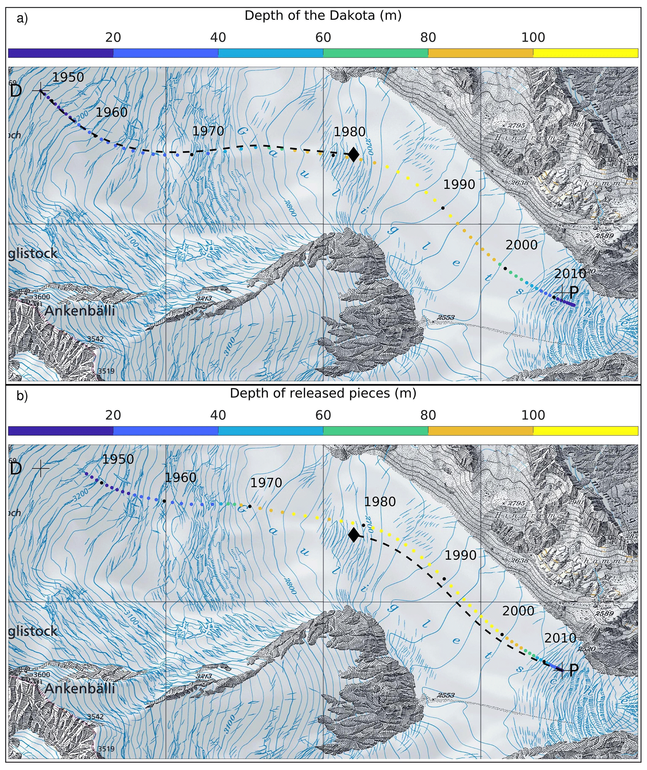
Figure 10 Topographic map of Gauligletscher with 1 km grid spacing showing the modeled horizontal trajectory of (a) the main body of the Dakota from 1947 to 2019 after integrating the modeled velocity field forward in time; and (b) the airplane pieces released from 2018 to 1947 after integrating the modeled velocity field backward in time. In both cases, we used the best-guess model run (Fig. 4). The corresponding forward (or backward) trajectory and its end position in 2019 (or 1947) computed by Compagno et al. (2019) is shown with a dashed line and a diamond symbol in panel (a) (or (b)) for comparison purposes. The location where the Dakota airplane crash-landed in 1946 and where pieces of the plane emerged in 2018 at the surface are indicated by the letters “D” and “P”, respectively. Reproduced by permission of swisstopo (BA20081).

Our new estimate still upholds the fact that certain pieces of the aircraft (e.g., one engine) became dislodged from the fuselage in 1947, which explains why each component followed a different trajectory. However, it refutes the theory that the wreckage, which had already been found, was moved far away from the main fuselage in 1947 (Compagno et al., 2019). Indeed, integrating the modeled velocity field backward in time starting from the location where wreckage was found in 2018 yields a trajectory that is slightly shorter but comparable to the one obtained by forward-in-time integration (Fig. 10, compare panels a and b). By contrast, the backward and forward trajectories computed by Compagno et al. (2019) were significantly different (Fig. 10, compare dashed lines in panels a and b). If the model were free of any numerical or physical errors, and if the entire Dakota aircraft had been released from the ice in 2018, then the two trajectories (forward and backward) would coincide. Therefore, the trajectory discrepancy can be understood as a measure of combined model errors and the distance between the body of the Dakota and the pieces dislodged from it in 1947. The relative minor discrepancy between trajectories from the new model shows that the Dakota main body and the pieces most likely always remained in close proximity to one another.

Among the five other selected model runs (Fig. 4), two show a very similar trajectory (with 2019 positions lying with a maximal distance of 100 m; see Figs. 10 and 11). Conversely, the three other model runs that use parameter A=150 MPa⁻³ a⁻¹ show shorter trajectories with end positions 300 to 500 m from the position of the released pieces (Fig. 11). This discrepancy (up to 20 % of the trajectory) is caused by slower velocities of the airplane in the early stage in the highest area. Indeed, sliding is nearly suppressed in the accumulation zone (i.e., c_u is close to zero, Fig. 4) as a result of the calibration procedure in the case of the softest ice A=150 MPa⁻³ a⁻¹ in order to maintain the ice flux. In other words, the higher vertical deformation rate of ice is compensated by the lower basal motion. Therefore, the ice velocities are low in the early stage of the movement of the submerged aircraft such that it takes longer for it to travel to a fast-moving area, a fact which causes discrepancies in the calculated trajectory length. This reveals the sensitivity of our trajectory estimate to uncertain parameters and shows that an error margin of several hundreds of meters should be taken into account (Fig. 11).

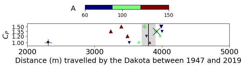
Figure 11 Distance traveled by the Dakota main body along the trajectory line drawn in Fig. 10a for the 12 model runs. The vertical line shows the average position of the pieces that were found in 2012, 2015 and 2018, and the shaded area shows its confidence taking into account the delay between the findings and the spread of the objects. Symbols + and × designate the results from the original model by Compagno et al. (2019), and the best-guess model run among the 12 (Fig. 4), respectively. Large (or small) symbols indicate the parameter sets that yielded realistic (or unrealistic) results and then were kept (or discarded) for analysis.

As well as the modeling results, we also computed the backward trajectory by integrating the observed horizontal velocity field (Fig. 3a), assuming the flow field in the current era times (here 2015–2019) to be representative of the 1947–2018 period. As a result, we found a backward trajectory (not shown) very similar to the one obtained by Compagno et al. (2019) as depicted in Fig. 10b. This trajectory is therefore unrealistically too short (by a factor of approx. 2). This simple estimate – whose advantage is to be free of any modeling considerations – fails because ice flow was significantly faster in the past; however, no direct observation is available to take this into account. This illustrates the incontrovertible superiority of an ice flow model that integrates information on the long-term ice motion (such as Lagrangian data used here) to reliably model the space–time trajectory followed by ice particles.

7 Conclusions

In this study, we successfully used plutonium and uranium contamination in an Alpine glacier induced by the 1950s and 1960s atmospheric nuclear weapon tests to date the ice of its ablation zone. While this tracer has been used multiple times for dating ice cores and other archives, this is the first time it has been used to date ice transported within the gravitational flow of ice to the ablation area, and which might have been deteriorated by temperate conditions and/or percolation water. Here we showed that the signal is still well preserved and that well-known activity peaks (i.e., 1963) can be identified, giving rise to positions that are in line with the observed ice flow of Gauligletscher. The combination of radionuclide contamination, state-of-the-art ice flow and mass balance modeling allowed us to derive a complete age map with an unprecedented degree of accuracy for a mountain glacier – a technique that is applicable to other glaciers. Our study sheds light on the potential of our method in two different ways:

• Radionuclide-based tracers provide invaluable data for model calibration as they integrate information on the long-term ice dynamics and mass balance over the entire glacier. In particular, they contain data from the past seven decades that are still observable today. Such Lagrangian data outperform the sparse surface ice velocities and mass balance data that are usually only available and used for that purpose. Therefore, they can much better constrain the model input parameters as illustrated here by the substantial bias between the former and the revised model results. Yet accurately tuning ice flow and mass balance parameters is essential to reliably model the future evolution of glaciers with a fair uncertainty range, especially in the context of global glacier retreat in a changing climate regime.

• The accurate and complete mapping of the age of ice is highly relevant to perform “horizontal ice cores”, i.e., for sampling surface ice of the past chronologically without having to perform expensive and logistically complex deep ice-core drilling. Note, however, that only a limited number of proxies traditionally used in high-alpine ice cores are expected to remain identifiable at the glacier surface because of alterations due to ice thermo-mechanical changes. Here isochrones were found to be nearly aligned with the flow near the north-west side, and very tight towards the sides, which called for the revision of our sampling strategy. Indeed, sampling in the lateral direction (i.e., orthogonal to the isochrones) would facilitate the identification of the double-peak structure in this region, and subsequently facilitate the derivation of an age–location relationship. Last, our dating method could also serve to identify the origin of any relics that have been transported by ice flow over decades and been released by the ice and found at the surface.

Furthermore, by including the radioisotope-based dating, it becomes possible to improve our estimate of the emergence time and position of the Dakota airplane, which crash-landed on Gauligletscher in 1946 and is still trapped within the ice. Indeed, the revised model shows that the Dakota is most likely going to emerge rather soon downstream from the place where pieces have been found recently.

Appendix A: Surface observed velocities

To estimate of the surface velocity of Gauligletscher, we used the MATLAB toolbox ImGRAFT (Messerli and Grinsted, 2015) to derive ice displacement fields by template matching (here we used normalized cross-correlation techniques) of satellite yearly-spaced pairs of ortho-images between 2015 and 2019. Artifacts were filtered based on signal-to-noise ratio, velocity magnitude or direction, and consistency between data sets (obtained from pairs 2015–2016, 2016–2017, 2017–2018, 2018–2019) assuming constant dynamics during the period 2015–2019. Note that we only used ortho-images of the end of the melt season to minimize the snow-covered areas where features can hardly be detected. The final velocity field (Fig. 3) was obtained by taking the median value between the data sets when the standard deviation was found to be sufficiently small. The velocity data cover the ablation area only as the accumulation area does not show enough features to apply the tracking algorithm. Note that the resulting observed velocities were found to be consistent with another independent data set (Dehecq et al., 2019) based on repeat-image feature tracking (Dehecq et al., 2015).

Appendix B: Error pattern between modeling and observations

To visualize the model inaccuracy that remains after calibration, we display the spatial error of the modeled ice surface by comparing to the available DEMs (1980 and 2010) in Fig. B1. As a result, the calibration tends to reduce the misfit on average (with an overall balance between the accumulation and ablation areas); however, the error pattern clearly shows local peaks, which likely reflect terrain heterogeneities and/or the incompetence of the model to capture small-scale features.

Figure B1 Modeled minus observed surface ice in 1980 (top panel) and 2010 (bottom panel) obtained with the best-guess model parameter set (Fig. 4), i.e., with A=100 and C_P=1.35. The corresponding root mean square error (RMSE) is given in Fig. 7a–b. Reproduced by permission of swisstopo (BA20081).

Appendix C: Sample preparation

C1 Reagents and equipments

All reagents were of analytical grade. Ultrapure water (18.2 MΩcm, Barnstead), 65 % nitric acid per analysis (prepared on a quartz sub-boiling apparatus), 40 % hydrofluoric acid Suprapur, 37 % hydrochloric acid Suprapur and ammonium iron (II) sulfate hexahydrate pro analysis (all from Merck) were used for the analyses. Standard solutions of U, Th and Indium (all from Alfa Aesar, Germany) were used to determine the correction factors due to tailing and hydroxide formation. U isotope standard IRMM-187 and IRMM-184 (all from Joint Research Centre, Belgium) were used for isotope ratio calibration and validation. A standard solution of ²⁴²Pu was used as radiochemical yield tracer. The extraction chromatography resins TEVA and UTEVA were obtained from Triskem International (Bruz, France). All the resins have 100–150 µm particle sizes. All separations were made with a vacuum box. All measurements were performed on a multicollector inductively coupled plasma mass spectrometer (MC-ICP-MS, Neptune, Thermo Fisher).

C2 Separation of iron hydroxide precipitation

To 1 kg of water, 300 µL of ²⁴²Pu radiochemical yield tracer (conc. 1.10⁻¹² g g⁻¹) and 240 mg of FeCl₃ (hexahydrate) was added. The mixture was warmed up and stirred at 60 ^∘C for 30 min. Ammonia (25 % aq. solution) was added until pH 8 was reached. After 30 min, the mixture was cooled down and allowed to precipitate. The supernatant was extracted by suction, the precipitate was transferred and centrifuged, and the supernatant was again extracted by suction. The precipitate was dissolved with HNO₃ (30 mL, 4.5 M) before (NH₄)₂ Fe(SO₄)₂ ⋅ H₂O (500 mg) was added. The solution was vigorously shaken and allowed to stand for 10 min. Pu and U were separated sequentially on a TEVA and UTEVA extraction chromatography resin.

C3 Separation of plutonium

The TEVA column was conditioned with 10 mL of a 0.2 % HNO₃ ∕ 0.002 % HF ∕ 0.01 mM Fe(II) solution and then with 10 mL of 3 M HNO₃ ∕ 0.1 mM Fe(II) solution. After loading the sample, the TEVA column was rinsed with 25 mL of 6 M HCl (remove Th) and then with 50 mL of 3 M HNO₃ ∕ 0.1 mM Fe(II) solution. The Pu fraction was eluted with 20 mL of a 0.2 % HNO₃ ∕ 0.2 % HF ∕ 0.01 mM Fe(II) solution and measured with MC-ICP-MS.

C4 Separation of uranium

The UTEVA column was conditioned with 10 mL of a 0.2 % HNO₃ solution and then with 5 mL of 3 M HNO₃ solution. After loading the breakthrough from the TEVA column, the UTEVA column was rinsed with 10 mL 6 M HCl and 10 mL 3 M HNO₃. The U fraction was eluted with 20 mL of 0.2 % HNO₃ ∕ 0.002 % HF solution.