the Creative Commons Attribution 4.0 License.
the Creative Commons Attribution 4.0 License.
 | 18 Nov 2020
Distribution and seasonal evolution of supraglacial lakes on Shackleton Ice Shelf, East Antarctica
Jennifer F. Arthur
Chris R. Stokes
Stewart S. R. Jamieson
J. Rachel Carr
Amber A. Leeson
Supraglacial lakes (SGLs) enhance surface melting and can flex and fracture ice shelves when they grow and subsequently drain, potentially leading to ice shelf disintegration. However, the seasonal evolution of SGLs and their influence on ice shelf stability in East Antarctica remains poorly understood, despite some potentially vulnerable ice shelves having high densities of SGLs. Using optical satellite imagery, air temperature data from climate reanalysis products and surface melt predicted by a regional climate model, we present the first long-term record (2000–2020) of seasonal SGL evolution on Shackleton Ice Shelf, which is Antarctica's northernmost remaining ice shelf and buttresses Denman Glacier, a major outlet of the East Antarctic Ice Sheet. In a typical melt season, we find hundreds of SGLs with a mean area of 0.02 km2, a mean depth of 0.96 m and a mean total meltwater volume of 7.45×10⁶ m3. At their most extensive, SGLs cover a cumulative area of 50.7 km2 and are clustered near to the grounding line, where densities approach 0.27 km2 km−2. Here, SGL development is linked to an albedo-lowering feedback associated with katabatic winds, together with the presence of blue ice and exposed rock. Although below-average seasonal (December–January–February, DJF) temperatures are associated with below-average peaks in total SGL area and volume, warmer seasonal temperatures do not necessarily result in higher SGL areas and volumes. Rather, peaks in total SGL area and volume show a much closer correspondence with short-lived high-magnitude snowmelt events. We therefore suggest seasonal lake evolution on this ice shelf is instead more sensitive to snowmelt intensity associated with katabatic-wind-driven melting. Our analysis provides important constraints on the boundary conditions of supraglacial hydrology models and numerical simulations of ice shelf stability.
Please read the corrigendum first before continuing.
-
Notice on corrigendum
The requested paper has a corresponding corrigendum published. Please read the corrigendum first before downloading the article.
-
Article
(20251 KB)
- Corrigendum
-
Supplement
(963 KB)
-
The requested paper has a corresponding corrigendum published. Please read the corrigendum first before downloading the article.
- Article
(20251 KB) - Full-text XML
- Corrigendum
-
Supplement
(963 KB) - BibTeX
- EndNote


Supraglacial lakes (SGLs) are widespread around the margins of Antarctica and can influence ice shelf dynamics both directly and indirectly (Arthur et al., 2020a; Kingslake et al., 2017; Stokes et al., 2019). Ice shelves flex when SGLs pond and drain on their surfaces, which can weaken them and make them more prone to break-up (Banwell et al., 2013, 2019; Banwell and MacAyeal, 2015). An often-cited example of this was the appearance and abrupt drainage of > 3000 SGLs on the surface of the Larsen B Ice Shelf in 2002 in the days preceding its collapse (Glasser and Scambos, 2008; Leeson et al., 2020), triggering a chain reaction of SGL hydrofracture and drainage events (Banwell et al., 2013; Robel and Banwell, 2019). SGLs can indirectly influence ice shelf dynamics by lowering surface albedo, which can intensify surface melt and induce a warming effect on the adjacent ice column (Lüthje et al., 2006; Tedesco et al., 2012; Hubbard et al., 2016). SGLs can also act as reservoirs by storing meltwater for crevasse penetration and hydrofracture (Scambos et al., 2000, 2003, 2009). Thus, the evolution and interaction of SGLs on ice shelves has important consequences for the stability of ice shelves, many of which exert a buttressing effect on inland ice flow (Fürst et al., 2016).
Recent research has shown SGLs form part of active surface meltwater systems on the surface of numerous Antarctic outlet glaciers and ice shelves (Banwell et al., 2019; Bell et al., 2017; Langley et al., 2016; Lenaerts et al., 2017; Moussavi et al., 2020; Kingslake et al., 2017; Stokes et al., 2019) and are particularly widespread on the Antarctic Peninsula and around the margins of the East Antarctic Ice Sheet (Arthur et al., 2020a; Kingslake et al., 2017; Stokes et al., 2019). However, few studies have conducted detailed analyses of the seasonal behaviour and spatial distribution of SGLs on ice shelves in East Antarctica. As such, direct observations of lake interactions and drainage are currently constrained to a limited number of ice shelves (Banwell et al., 2019; Bell et al., 2017; Langley et al., 2016; Liang et al., 2019; Moussavi et al., 2020; Kingslake et al., 2015), and our understanding of the importance of SGL evolution on ice shelf instability remains limited.
Here, we focus on Shackleton Ice Shelf, which is East Antarctica's sixth-largest and most northerly remaining ice shelf in Antarctica (Rignot et al., 2013; Zheng and Zhou, 2019). Over 70 % of the ice shelf area exerts a buttressing effect on the major outlet glaciers flowing into it, and a number of ice rises and islands act as pinning points for the ice shelf (Fürst et al., 2016; Fig. 1). The remaining 30 % of the ice shelf has been identified as passive shelf ice, i.e. that could be removed without the acceleration of inland ice (Fürst et al., 2016). The ice shelf is fed by Denman Glacier, whose catchment holds ice equivalent to ∼ 1.5 m of sea level and is ∼ 1.9 times larger than the catchment of Pine Island Glacier (Morlighem et al., 2019; Stephenson and Zwally, 1988; Willis et al., 2016). Portions of the ice shelf experience high mean surface melt rates (> 200 mm w.e. yr−1) compared to other parts of coastal East Antarctica, such as the Fimbul (> 80 mm w.e. yr−1), Riiser-Larsen (> 70 mm w.e. yr−1), Nivlisen (> 80 mm w.e. yr−1) and Roi Baudouin (> 150 mm w.e. yr−1) ice shelves (Trusel et al., 2013). High densities of SGLs in the ice shelf grounding zone suggest that it contains ice-saturated firn (Alley et al., 2018; Lenaerts et al., 2017). The combination of its topographic setting, intense surface melting and low firn air content (FAC) makes Shackleton Ice Shelf potentially vulnerable to hydrofracturing (Alley et al., 2018; Stokes et al., 2019).
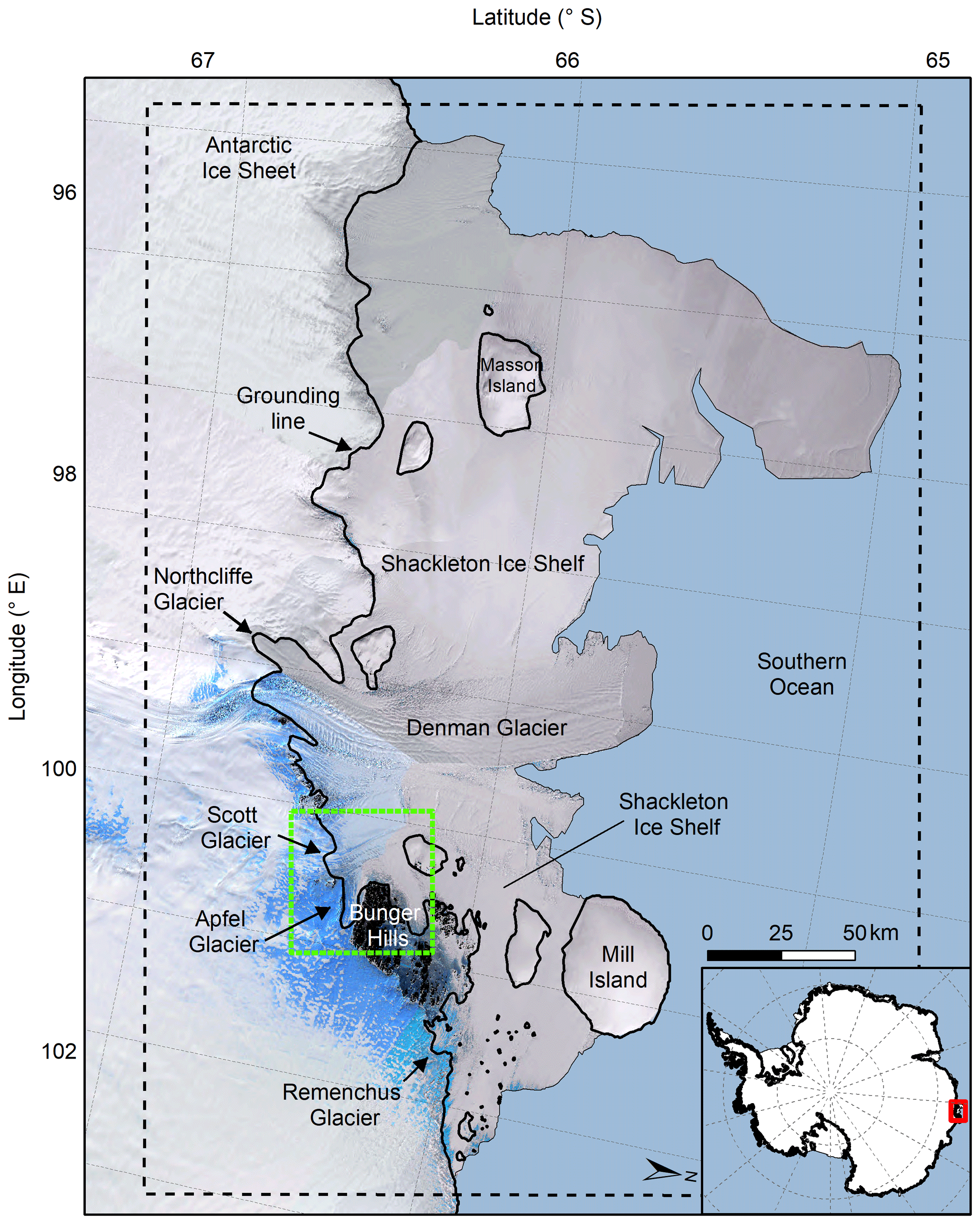
Figure 1Overview map of Shackleton Ice Shelf with LIMA (Bindschadler et al., 2008) in the background. The grounding line (thick black line) is taken from Rignot et al. (2016). The subset area used for detailed analysis of lake area and depth extractions is outlined in green, and the dashed black box outlines the area used to extract ERA5 reanalysis near-surface air temperature. The light-blue areas visible on the ice sheet are blue-ice areas.
Our overall aim is to investigate the long-term distribution and evolution of SGLs on Shackleton Ice Shelf. Our first objective is to analyse the intra-seasonal and inter-seasonal evolution in the spatial distribution, extent and volume of SGLs over multiple melt seasons from 2000 to 2020 using remote sensing. Our second objective is to explore potential glaciological and climatic controls on SGL formation and distribution on this ice shelf in order to improve our understanding of its potential vulnerability.
Shackleton Ice Shelf, in Queen Mary Land, East Antarctica (65∘ S, 100∘ E), covers an area of 33 820 km2 (Zheng and Zhou, 2019; Fig. 1). Denman Glacier flows into the ice shelf at speeds over 1800 m yr−1 at its grounding line (Rignot et al. 2019) and occupies a trough deeper than 3500 m b.s.l. which connects to the Aurora Subglacial Basin (Morlighem et al., 2019; Roberts et al., 2011). Denman Glacier has accelerated 16 % since the 1970s (Rignot et al., 2019) and is thinning inland (Flament and Rémy, 2012) and undergoing grounding-line retreat (Konrad et al., 2018). The ice shelf surface flow has accelerated by 43 % between 1957 and 2016 (Rignot et al., 2019). Several smaller outlet glaciers drain into the ice shelf, including the Scott, Apfel, Remenchus and Northcliffe glaciers (Fig. 1). The Bunger Hills (a large nunatak) and an extensive blue-ice area lie adjacent to the ice shelf grounding zone (Fig. 1). Ice thickness varies across the ice shelf from 231 m (at the calving front) to < 10 m around Mill Island (Fretwell et al., 2013; Wearing et al., 2015). Thinning of Shackleton Ice Shelf at a rate of 0.12 m yr−1 between 2003 and 2008 has been attributed to enhanced basal melting (Pritchard et al., 2012). SGLs on Shackleton Ice Shelf have been previously mapped for the year 2015 from Landsat 8 imagery, to assist interpretation of snowmelt detection from microwave radiometer and scatterometer data (Zheng and Zhou, 2019), but no studies of seasonal and/or interannual SGL evolution currently exist for the ice shelf.
3.1 Satellite imagery acquisition and processing
For the years between 1974 and 2020 we acquired all imagery from the Landsat 1, 4 and 5 MSS (Multispectral Scanner System) and TM (Thematic Mapper); Landsat 7 ETM+ (Enhanced Thematic Mapper); Landsat 8 OLI (Operational Land Imager); and Sentinel-2A and Sentinel-2B MSI (MultiSpectral Instrument) over Shackleton Ice Shelf during the austral summer months (November to February) with ≤20 % cloud cover from the USGS EarthExplorer (https://earthexplorer.usgs.gov, last access: February 2020) and the European Space Agency Copernicus Open Access Hub (https://scihub.copernicus.eu/dhus, last access: February 2020; Table S1 in the Supplement). For scenes that included cloud cover below the ≤ 20 % threshold, cloud cover was mostly restricted to the outermost parts of the ice shelf or further inland beyond the grounding line, where cloud-free scenes indicated that no lakes form. Eight scenes with cloud cover higher than 20 % were used, where cloud cover did not obscure most of the ice shelf and SGLs were visible. These were used to analyse the spatial distribution of lakes across the ice shelf but were not used in our analysis of lake area and volume (Sect. 3.3). The multispectral bands of the Landsat 8 images were pan-sharpened to 15 m using the panchromatic Band 8 and a Brovey transform (Gillespie et al., 1987) in QGIS. For more recent years (2017 to 2019), Sentinel-2A and Sentinel-2B imagery was used in preference to Landsat 8 or another sensor, such as the Moderate Resolution Imaging Spectroradiometer (MODIS) or Advanced Spaceborne Thermal Emission and Reflectance Radiometer (ASTER), owing to its high spatial resolution (10 m) and revisit period of 5 d, though Landsat 8 imagery was used where no Sentinel-2 imagery was available with suitable (≤ 20 %) cloud cover.
It is important to remove the influence of different satellite imagery acquisition conditions before extracting SGL extents and depths. To do this, digital numbers were converted to top-of-atmosphere (TOA) reflectance for red and blue bands using DOS1 (dark-object subtraction) atmospheric correction (Moran et al., 1992) in QGIS and the scene-specific metadata file containing reflectance multiplicative and additive scaling factors and the solar elevation angle. This process removes the cosine effect at different solar zenith angles (due to different scene time acquisitions) and compensates for differences in solar irradiance.
3.2 Automated mapping of SGL extent
We used the normalised difference water index (NDWI) adapted for ice (Yang and Smith, 2013) to classify pixels as “water” or “non-water” (i.e. ice, snow, exposed bedrock or ocean) following Eq. (1):
This version of the NDWI has been widely applied for mapping surface meltwater in Antarctica (Arthur et al., 2020a; Banwell et al., 2019; Bell et al., 2017) and Greenland (Doyle et al., 2013; Williamson et al., 2017; Yang and Smith, 2013). We found NDWIice produced fewer false SGL classifications over blue-ice and slush areas than with other versions of the NDWI, such as those using the near-infrared band (Fig. S1).
The first step in our procedure for mapping SGLs was to apply a bedrock mask derived from Landsat 8 data (Burton-Johnson et al., 2016). Exposed bedrock appears spectrally similar to water in the red band, so masking bedrock avoids misclassification of rock as water. This was particularly important in our study given the large area of nunataks (Bunger Hills) adjacent to the ice shelf. After rock masking was performed, we applied an NDWI threshold value of 0.25, following previous studies (Banwell et al., 2019; Bell et al., 2017; Dell et al., 2020; Doyle et al., 2013; Williamson et al., 2017; Yang and Smith, 2013), meaning pixels with NDWIice > 0.25 were assumed to be water-covered. This threshold was found to be the most appropriate for detecting lakes, apart from in 11 scenes, where the threshold value was manually tuned in 0.01 increments to improve SGL identification by including pixels which were visibly water-covered in true-colour composites of the area (Table S1).
Once an NDWI threshold value was applied, each image was reclassified into a binary image and vectorised (converted to polygon shapefiles). Clouds were masked by manually inspecting each RGB image and deleting any cloud. Some manual editing of SGL extents was necessary where floating ice in the centre of SGLs had resulted in pixels being misclassified as water. The transition from melting ice to saturated firn, slush, shallow ponds and deeper SGLs makes it challenging to adopt a clear binary definition of “lake” versus “non-lake” (Dell et al., 2020). To account for this uncertainty we used a minimum size threshold of 2 pixels, in order to remove very small SGLs likely comprised solely of mixed pixels (i.e. pixels containing a combination of water, slush and/or snow or ice; 200 m2 for Sentinel-2, 450 m2 for Landsat 7 and 8, 1800 m2 for Landsat 4 and 5, 7200 m2 for Landsat 1), following previous studies (Moussavi et al., 2020; Pope et al., 2016; Stokes et al., 2019). For the purposes of our study, we chose not to classify SGLs separately from supraglacial meltwater channels, given the ambiguity in distinguishing between channels and thin, elongate SGLs.
Finally, NDWI classifications were checked against RGB composites and false positives, including small bedrock outcrops not included in the bedrock mask. Dark crevasses were also manually removed. To further reduce noise and improve the visual clarity of the dataset, we then applied the dissolve function in ArcMap to clean up overlapping pixels and the aggregate tool to combine pixels within a distance of 2 pixels. Apart from potentially reducing large numbers of very small SGLs, these changes were largely cosmetic and are insignificant in terms of the uncertainties associated with identifying SGLs and calculating total SGL area, described in Sect. 3.4.
3.3 Extracting lake depths and volumes
We applied a physically based radiative transfer model to calculate the water depth of all pixels classified as lake (Pope, 2016; Pope et al., 2016; Sneed and Hamilton, 2007). This method calculates lake water depth (z) using the rate of light attenuation in water, lake-bottom albedo and optically deep water reflectance (Philpot, 1989) following Eq. (2):
where Ad is lake bed reflectance, R∞ is the reflectance of optically deep water, Rz is the reflectance value of a water-coloured pixel and g is the attenuation coefficient rate.
The radiative transfer model was applied to a subset area of the ice shelf (48 km × 48 km; Fig. 1) to allow lake depth comparisons between years with different satellite imagery coverage. This subset area was selected as the region in which most SGLs were concentrated during each melt season with consistent coverage of cloud-free imagery, enabling us to extract changes in lake area and depth on both the floating ice shelf and the grounded ice upstream of its grounding line. Lake area and depth statistics presented in Sect. 4 are all extracted from this subset area. We excluded nine image scenes from our analysis which did not fully cover this subset area, to maintain full comparability between individual dates. Issues with cloud cover resulted in only one useable scene during some melt seasons and no suitable imagery in others (2002, 2004–2006; Table S1).
Ad was calculated image by image by extracting the mean reflectance of a 2-pixel buffer around each lake polygon. This is an improvement on previous approaches which used static Ad values across a region (e.g. Sneed and Hamilton, 2007). The reflectance value immediately beyond identified lake areas is assumed to be comparable to the lake bed if it were at the surface (Pope et al., 2016). R∞ is typically approximated as the pixel reflectance from open ocean water. Most scenes used in this study did not contain optically deep water, and we found the average difference between using an R∞ of zero and using R∞ values averaged from 15 nearby scenes to be < 10 % (Supplement). Therefore, we used an R∞ of zero for all scenes, following MacDonald et al. (2018) and Banwell et al. (2019).
Red light attenuates more strongly in water than blue light, meaning that there are larger measurable changes in red reflectance over water than for other wavelengths (Box and Ski, 2007; Pope et al., 2016). For Sentinel-2 scenes, we used red (Band 4) reflectances for Rz and a g value of 0.8304, following Williamson et al. (2017). For Landsat 8 scenes, we followed the recommendation of Pope et al. (2016) and took an average of the depths calculated using the red-band (Band 4) and panchromatic-band (Band 8) TOA reflectances, using g values of 0.7507 and 0.3817 respectively. For Landsat 7 ETM+ scenes, we used red (Band 3) reflectances for Rz and a g value of 0.8049 following Pope et al. (2016). We are unable to calculate lake depths before the year 2000 (i.e. from Landsat 1 MSS, Landsat 4 TM and Landsat 5 TM scenes) using this physically based depth method because lab-based absorption coefficients within the full red-band wavelength ranges (Pope and Fry, 1997) are unavailable. Lake depths within the subset area were extracted using zonal statistics in ArcMap. Lake volumes were calculated by multiplying each pixel area by its calculated water depth within the lake boundaries.
3.4 Errors and uncertainties in extracting lake areas and depths
We quantified the uncertainties in our mapping technique by quantitatively comparing SGL areas derived from NDWI with those derived from manual digitisation in four sample areas (Fig. S2a–d). The smaller SGLs (< 0.01 km2) generated the largest percentage differences, and we found a mean absolute error of 0.007 km2 and a root mean square error of 0.029 km2 between manually digitised SGL areas and those derived from NDWI. We attribute this to manual digitisation being less conservative at “diffuse”, less well defined SGL edges. Despite these differences, we found very close agreement between the two methods (R2=0.979, p=0.006). We also quantified the impact of sensor resolution on lake detection and lake extents and found there is generally a very good agreement between lake areas derived from Landsat 8 and Sentinel-2 (Fig. S3). We therefore assign a conservative uncertainty of 1 % to our total SGL area for each time step, following Stokes et al. (2019).
The depth–reflectance algorithm used to extract lake depths assumes that lake-bottom albedos are homogenous, that lake water contains minimal dissolved matter and that there is no scattering of light from the lake surface associated with wind-driven roughness (Sneed and Hamilton, 2007). We acknowledge that the last of these assumptions may not always hold if there are wind-driven surface waves. We also acknowledge that wind-blown sediment from the adjacent Bunger Hills rock outcrops could cause variability in lake-bottom albedo. This is known to be an important process on McMurdo Ice Shelf, which is heavily debris-covered due to sediment redistribution from medial moraine and rock outcrops (Glasser et al., 2014; MacDonald et al., 2019; Banwell et al., 2017, 2019; MacDonald et al., 2020). Where lakes were partially ice-covered, we could not calculate the depth of the central, probably deepest, regions of these lakes. In such cases, we calculated the depth of the outer ring of lake ice-free water, following Banwell et al. (2014). This is likely to underestimate the volumes of deeper lakes, but we record maximum lake volumes that are similar (i.e. not substantially lower) to those reported elsewhere in Antarctica (Bell et al., 2017; Banwell et al., 2014; Langley et al., 2016).
3.5 Extraction of lake elevations, slopes, densities and ice surface velocities
Lakes were classified as forming on grounded or floating ice using the Making Earth System Data Records for Use in Research Environments (MEaSUREs) grounding line which is derived from an average of differential interferometric synthetic-aperture radar (inSAR) data from 1992 to 2014 (Rignot et al., 2016). Although a more recent inSAR grounding line exists for parts of Denman and Apfel glaciers, derived from ERS-1, ERS-2 and Sentinel-1 data acquired in 1996, 2015 and 2017 (DLR, 2018), this is incomplete on Shackleton Ice Shelf, and the MEaSUREs grounding line was therefore used as the most recent continental-wide grounding line. Surface elevation and slope values were extracted from the Reference Elevation Model of Antarctica (REMA), which has an 8 m spatial resolution. Ice velocity values were extracted from the MEaSUREs InSAR-based ice velocity mosaic which was derived by averaging data covering the period 1996–2016 (Rignot et al., 2017). Lake area densities were calculated using lake polygon centroids as inputs to the Point Density tool in ArcMap. This tool calculates the cumulative area of SGLs within 1 km2 cells by dividing the total number of points that fall within a defined neighbourhood around each raster cell by the area of the neighbourhood. Stokes et al. (2019) apply this method across the East Antarctic Ice Sheet using a 50 km search radius. Here, a 20 km search radius was chosen as an appropriate size given the area of the ice shelf.
3.6 Extracting near-surface temperature, surface snowmelt and firn air content
To compare lake areas with surface climatological conditions, we used near-surface air temperature and modelled surface snowmelt. In the absence of any automatic weather stations within 80 km of Shackleton Ice Shelf (and hence any long-term meteorological observations within our 2000–2020 study period), we used monthly averaged near-surface temperature (2 m temperature) from the European Centre for Medium-Range Weather Forecasts ERA5 reanalysis from 1979 to 2019 as the best available option. We extracted near-surface temperature over a ∼262 km × 370 km box covering the whole ice shelf (Fig. 1). ERA5 reanalysis is provided at a 0.25∘ (∼ 31 km) resolution. To investigate whether timings of modelled snowmelt events and extensive SGL ponding were comparable, we extracted mean snowmelt over the ice shelf from daily surface melt flux outputs for the period 2000 to 2019 generated by the Regional Atmospheric Climate Model (RACMO) version 2.3p1, which has a horizontal resolution of 27 km. Details of the model can be found in Van Wessem et al. (2018). To investigate the relationship between lake areas and simulated firn air content (FAC), we extracted mean and minimum FAC (total integrated pore space, i.e. the thickness of the equivalent air column contained in the firn in metres) over the ice shelf from daily FAC for the period 2000 to 2019 generated by RACMO version 2.3p1.
3.7 Hydrological routing analysis
To estimate potential meltwater routing across the ice shelf surface (Leeson et al., 2012; Bell et al., 2017) and compare this to mapped distributions of SGLs, a D-infinity algorithm (Tarboton, 1997) was applied to a 100 m resolution version of the REMA DEM (clipped to Shackleton Ice Shelf). We calculated flow direction and accumulated flow into each cell after filling closed basins (sinks) in the DEM. The output raster was then vectorised to show the potential pathways of surface meltwater routing across the ice shelf once surface depressions have been filled.
4.1 Spatial distribution of SGLs
We find that SGLs tend to cluster around the ice shelf grounding zone, near exposed blue-ice areas and the Bunger Hills nunataks, whereas they are almost entirely absent towards the ice shelf calving front, where surface melt rates are highest (Trusel et al., 2015; Fig. 2a). Lakes form in particularly high densities on Scott, Apfel and Remenchus glaciers. Indeed, lake area densities reach their maximum (0.27 km2 km−2) on this portion of the ice shelf (Fig. 2b). No lakes form on the heavily crevassed tongue of Denman Glacier. On the ice shelf itself, most lakes are only recorded in a given position on a single date in a particular year, because they were advected downstream with ice flow (Fig. 2b–d). The largest recorded feature is an area of coalesced lakes covering up to 11.96 km2 which formed in January 2020 on Scott Glacier, alongside more linear, elongate lakes which occupy a ∼ 10 m deep longitudinal depression on the glacier surface (Fig. 2d). Further west, smaller lakes occupy crevasses in the suture zone between Denman and Scott glaciers (Fig. 2c). Though the spatial distribution of lakes on these parts of the ice shelf remains similar during each melt season, lakes gradually become advected downstream with ice flow each year (Fig. 2f).

Figure 2Recurrence frequency of lakes mapped between 1974 and 2020 on Shackleton Ice Shelf out of a total of 58 individual satellite scenes. Surface melt flux derived from QuikSCAT scatterometer (2000–2009 average from Trusel et al., 2013) on the portion of the ice shelf where lakes predominantly form (a). Lakes are concentrated in the grounding zone downstream of blue ice and adjacent to exposed rock (b and c). Lakes on the ice shelf itself are short-lived in a given location (d) and migrate down the shelf with ice flow over multiple melt seasons (f). Lakes on grounded ice upstream of the grounding line typically occupy fixed ice surface depressions and therefore frequently reform in the same locations during multiple melt seasons (e). Note the scale bar frequency corresponds to the number of times a lake was recorded in the available cloud-free satellite imagery, rather than to the number of years over this time period.
Upstream of the grounding line, lakes have a high tendency to reoccur annually in the same locations (Fig. 2d). Specifically, seven lakes upstream of Apfel Glacier were present in 62 % of scenes mapped (Fig. 2d). The area just upstream of this cluster of lakes represents the upper elevation limit (527 m a.s.l.) of recorded SGLs, 12.8 km inland from the grounding line (∼ 90 km from the coastline). Lakes only formed at this maximum elevation during the 6 melt years when total lake volume was highest (2010, 2014, 2015, 2017, 2018 and 2020; see Sect. 4.2).
The concentration of SGLs around the ice shelf grounding zone is reflected in their topographic distribution, which is strongly skewed towards low (≤ 10 m) elevations and low (< 1∘) ice surface slopes close to and just above the grounding line (Fig. 3a–b). SGLs preferentially form on slower-moving ice (< 50 m yr−1), typically occupying smaller tributary glaciers and suture zones between glaciers, rather than on fastest-flowing portions of the ice shelf like Denman Glacier (Fig. 3c). Lakes form in very close proximity to exposed bedrock (< 10 m) and are within or downstream of blue-ice areas around the ice shelf grounding line (Fig. 3d).
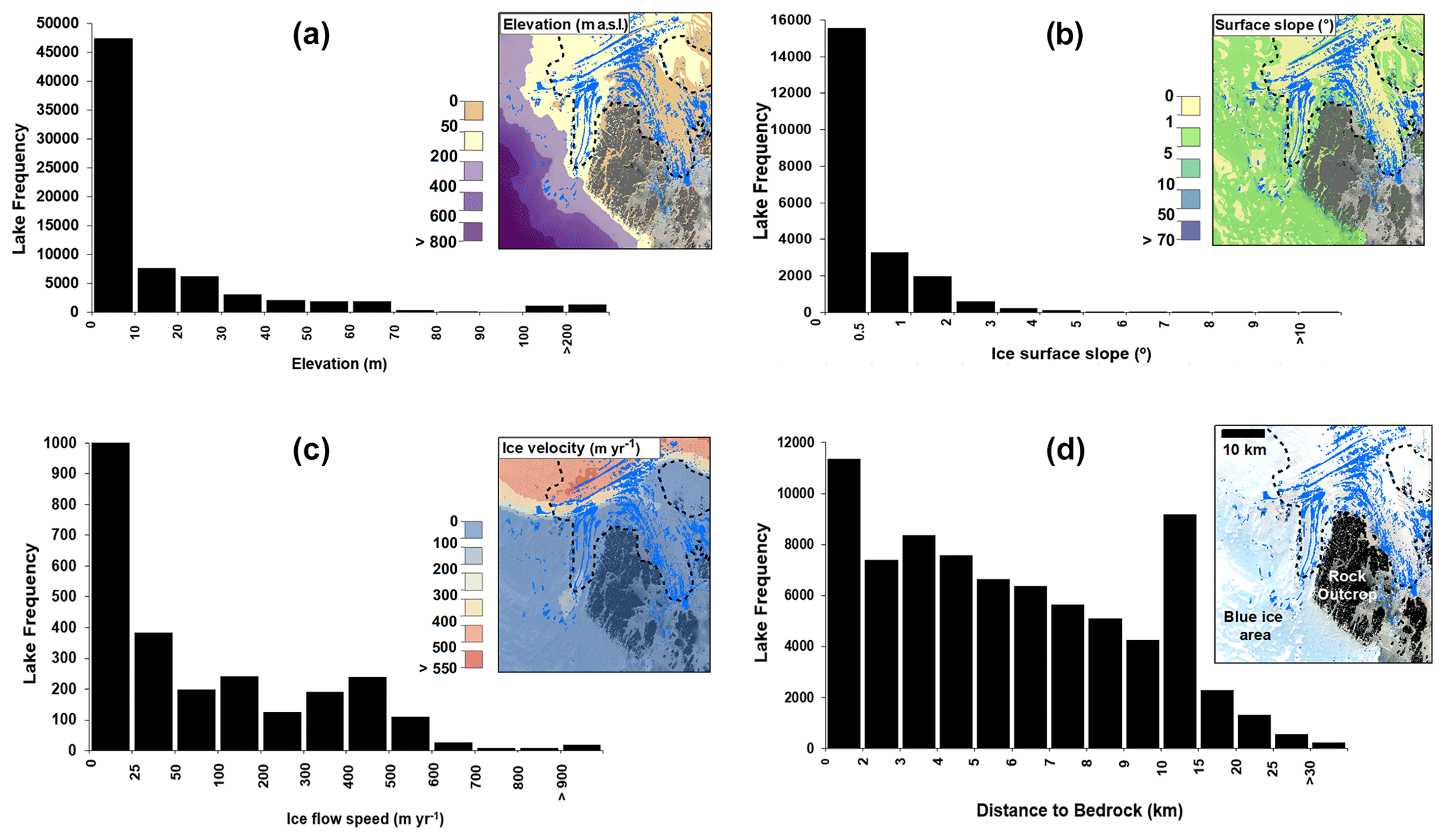
Figure 3Frequency distributions of supraglacial lakes on Shackleton Ice Shelf by topographic variables: (a) individual lake mean elevations, (b) ice surface slope of individual lakes, (c) ice flow speed, (d) distance of each lake to nearest exposed bedrock. The four panels show a subset of lakes (in blue) on the ice shelf and their spatial association with low elevations, low surface slopes, low ice flow speeds, and exposed rock or blue ice. The grounding line is represented by the dashed black line.
4.2 Seasonal evolution of SGLs
4.2.1 Intra-seasonal and inter-seasonal lake evolution
To investigate the seasonal behaviour of SGL formation and evolution on Shackleton Ice Shelf, we present time series of total lake area, depth and volume over the 2000–2020 melt seasons (Fig. 4). In a typical melt season, we observed hundreds (∼ 100–1000) of SGLs that were, on average, 0.02 km2 in area and 0.96 m deep and held an average total meltwater volume of 7.45×10⁶ m3. The earliest that meltwater starts being stored on the ice shelf surface within SGLs is in late November (Fig. 4, Table 1). This is earlier than has been reported in other regions of East Antarctica, where SGLs have been observed forming from mid-December but typically begin forming in early January (Langley et al., 2016; Leppäranta et al., 2013; Moussavi et al., 2020). We suggest the earlier onset of lake formation reflects an earlier start to the melt season due to the northerly location of this ice shelf.
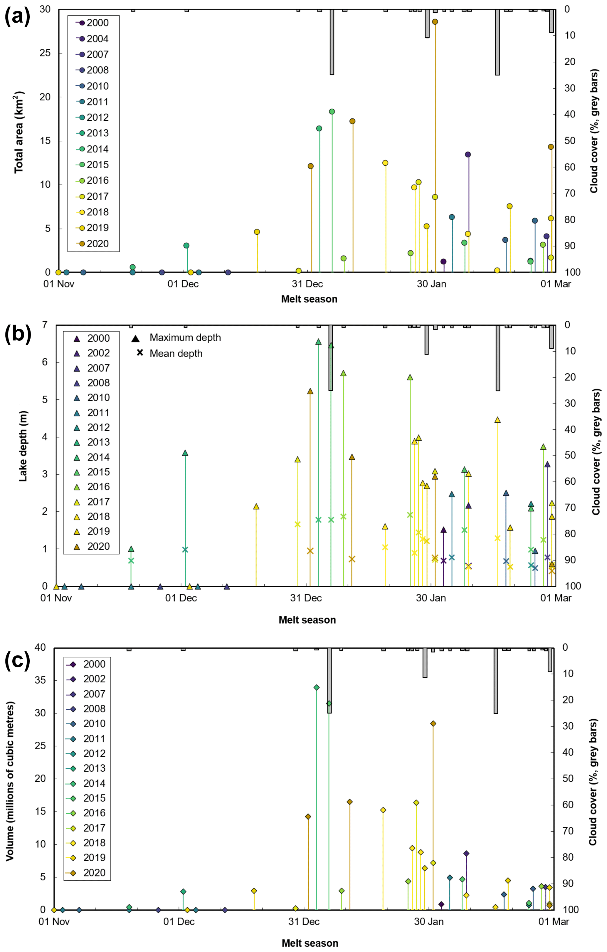
Figure 4Evolution of total lake area, depth and volume across Shackleton Ice Shelf over the 2000–2020 melt seasons. The stem plots present time series of meltwater area (a), depth (b) and volumes (c) of lakes inside the subset area (green box in Fig. 1), where each point and stem represent a single date of lake observations. Grey bars indicate the percentage of cloud cover within this subset area. Full lake area, depth and volume data for individual years are included in Table 1.
Table 1Total lake area and volume within the 48 km × 48 km subset area on Shackleton Ice Shelf.

Total lake area on the ice shelf increases through to December and January, peaks in early to late January (Fig. 4a), and then decreases through the remainder of the melt season until late February. Mean and maximum lake depths follow a similar seasonal pattern to lake area, and the deepest lakes are generally recorded between early January and mid-January (Fig. 4b). However, mean and maximum lake depths do not always peak simultaneously with lake area (Fig. 4b, Table 1). For example, in 2020, lake depth peaks 30 d before total lake area and volume peak on 1st January. SGLs on grounded ice upstream of the ice shelf have a higher mean depth of 0.94 m (SD is 0.68; p=0.01) compared to a mean depth of 0.91 m (SD is 0.54) on the ice shelf (Fig. S4). Total meltwater volumes remain low ( m3) during the months of November, December and February and peak between early to late January (Fig. 4c). In 2014, 2015 and 2020, lake volume was more than 2 standard deviations from the 2000–2020 mean. In 2020, total lake area also deviated by almost 3 standard deviations from the 2000–2020 mean (Fig. 5b). Total lake area was up to 3.9 times higher and total lake volume up to 4.5 times higher than the long-term mean in the 5 years 2014, 2015, 2017, 2018 and 2020. At the time of peak total lake volume during these years, lakes covered 0.05 %, 0.06 %, 0.03 %, 0.04 % and 0.09 % respectively of the total ice shelf area.
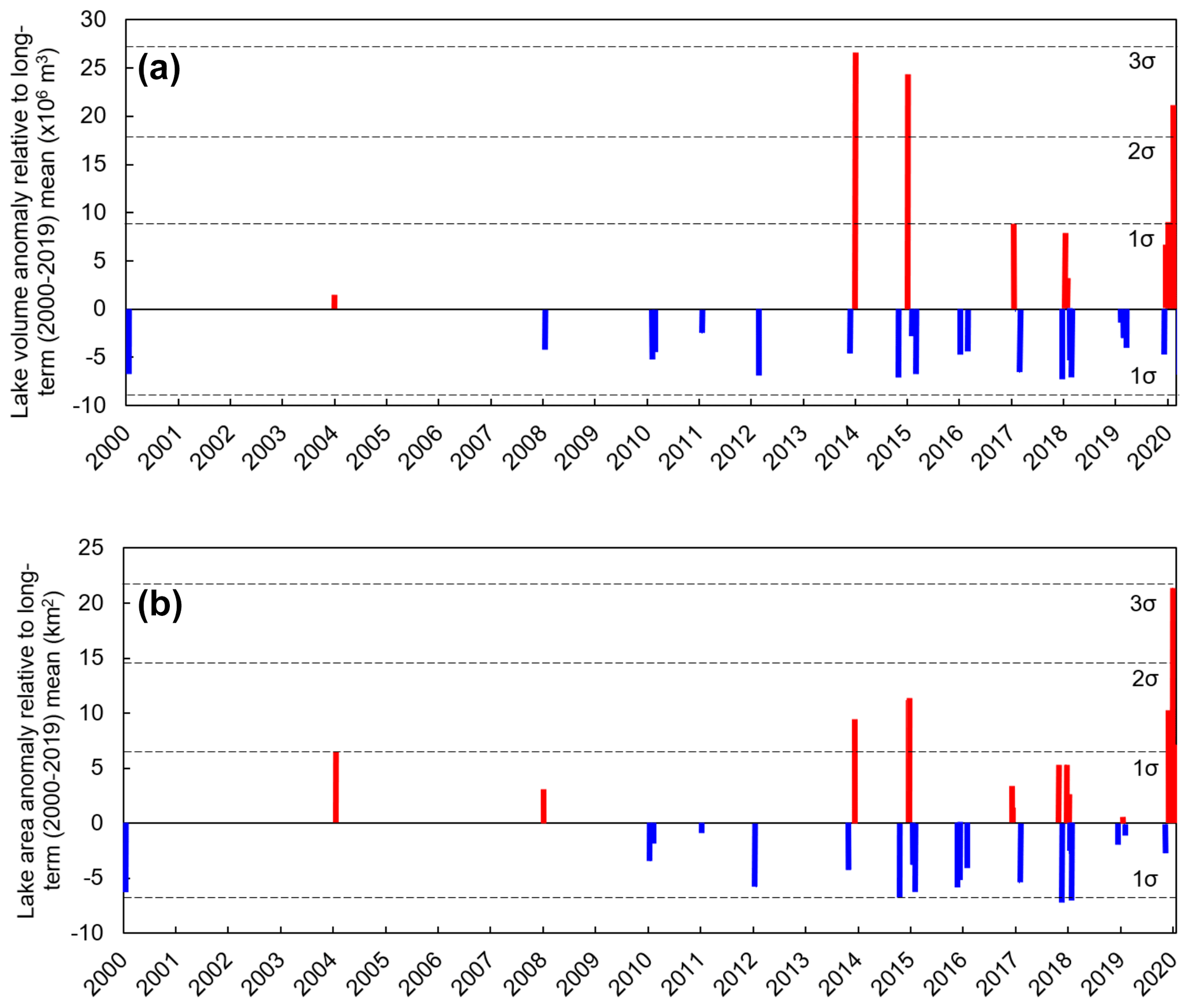
Figure 5Total lake volume anomaly relative to long-term (2000–2020) mean (a) and total lake area anomaly relative to long-term (2000–2020) mean (b). Dashed black lines represent 1, 2 and 3 standard deviations from the long-term mean.
We document lakes forming during the 3 years prior to 2000 where suitable imagery was available (1974, 1989 and 1991), though we were unable to include these in our depth and volume analyses (see Sect. 3.3). During these years, lakes occupy many of the same locations as in later melt seasons, including on Scott and Apfel glaciers and in a smaller blue-ice area near the northern part of the ice shelf grounding line. SGLs are less extensive during these years than in 2000–2020 (total area 20.3 km2, 5.6 km2 and 8.8 km2 respectively), though we note imagery was limited to the very start (early November) and end (late February) of the melt season.
4.2.2 Lake drainage events
We observe lakes disappearing in three ways: supraglacial drainage via channels over the ice surface, englacial drainage into the firn, or surface refreezing and/or snow burial (Fig. 6). Lakes commonly refreeze at the end of a melt season, indicated by relict frozen lake scars which are similar to refrozen lakes in previous studies (e.g. Langley et al., 2016; Leeson et al., 2020; Tuckett et al., 2019; Fig. 6a–c). This is the dominant mechanism of lake disappearance and is commonly preceded by ice “lids” that grow outwards from lake centres (Fig. 6a–c).
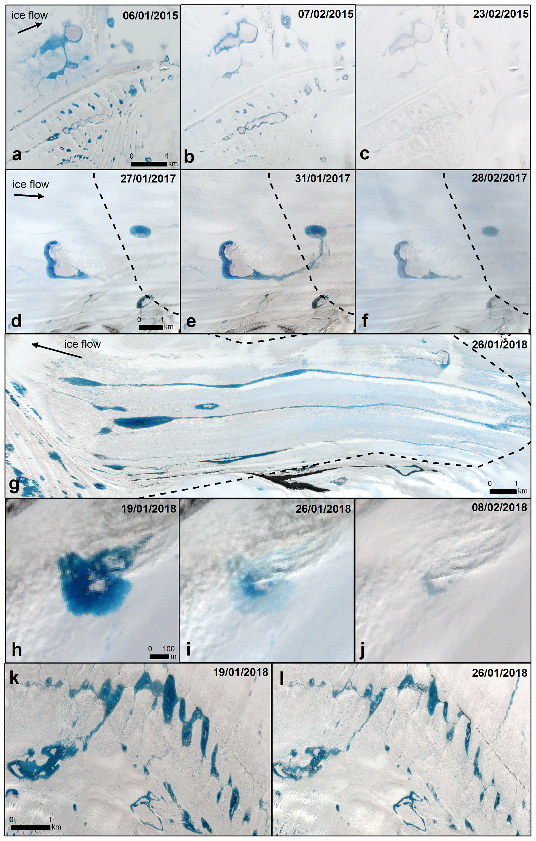
Figure 6Examples of lake drainage and refreeze–burial events on Shackleton Ice Shelf: lakes refreezing and becoming buried by snow (a–c), a lake draining via a supraglacial stream (d–f), supraglacial streams or rivers feeding lakes (g), a lake before and after through-ice drainage (h–j), and a chain of lakes partially draining in ≤7 d (k–l). Background images are Landsat 8 (a–c) and Sentinel-2A (d–l).
Earlier in the melt season, some lakes drained supraglacially into others via surface channels (Fig. 6d–f). During the peak of the melt season in some years, large portions of the ice shelf firn layer become saturated, causing meltwater to accumulate and coalesce in large lakes on portions of the ice shelf, such as on the tongue of Scott Glacier. This occurred when total lake area exceeded 10 km2 (in February 2004 and January 2014, 2015, 2017, 2018 and 2020). During these seasons of more extensive surface melt, supraglacial rivers develop by mid-January, fed by lakes upstream of the grounding line (e.g. Fig. 6g). The largest of these rivers reaches ∼ 14 km on Apfel Glacier, though these feed other lakes rather than exporting meltwater off the ice shelf edge as has been observed on Nansen Ice Shelf in Antarctica (Bell et al., 2017).
We also recorded several instances of lakes apparently draining englacially into the firn over a ≤7 d period during January 2018 and 2020 (Fig. 6h–l). For example, one chain of lakes (Fig. 9k–l) lost ∼ 36 % of their 2.2 km2 total area and ∼ 24 % of their 3.5×10⁶ m3 total volume in ≤ 7 d. If this chain of lakes had refrozen, we would have expected to record a reduction in area of the surrounding lakes. However, the surrounding lakes did not change in area over this period, suggesting they also did not refreeze. Neither did downstream lakes grow in size, and nor was this chain of lakes associated with any major streams or rivers which could have exported the meltwater supraglacially. Therefore, we make the interpretation that these lakes drained englacially into the firn. In other years, this same chain of lakes remains undrained and freezes over (as in Fig. 6a–c).
4.2.3 Lake evolution and relationship with climate
We compare total lake area during the 2000–2020 melt seasons with mean near-surface temperature extracted from ERA5 reanalyses to investigate the relationship between seasonal lake coverage and temporal fluctuations in air temperature on Shackleton Ice Shelf (Fig. 7). We find that warmer melt seasons do not necessarily correlate with more extensive lake coverage. For example, although 2019–2020 records the highest total lake area (28.55 km2), it has a lower mean December–January–February (DJF) near-surface temperature (−9.3 ∘C; Fig. 7c). Similarly, in January 2015 and 2014, the next most extensive lake years, mean DJF temperature was also low (−8.4 and −8.6 ∘C respectively), although lakes started to form earliest in the melt season (19 November 2015 and 2 December 2014; Fig. 7b). However, in the melt seasons with the five lowest mean DJF temperatures (1999–2000, 2007–2008, 2011–2012, 2012–2013 and 2015–2016), total lake area did not exceed 5 km2 (Table 2, Fig. 7b). Likewise, we recorded a relatively high maximum lake extent in 2016–2017 (10.29 km2), which was the melt season with the highest mean DJF temperature (−6.4 ∘C; Fig. 7c). Overall, from 2000 to 2020, total lake area is only weakly positively correlated with mean surface air temperature in the preceding part of the melt season, i.e. from 1 November to the date of lake observation (r2=0.15, p=0.04; Fig. 8). Therefore, peak years in lake coverage exhibit only a weak relationship with near-surface temperature, suggesting that other factors such as localised albedo interactions may act as more important controls.
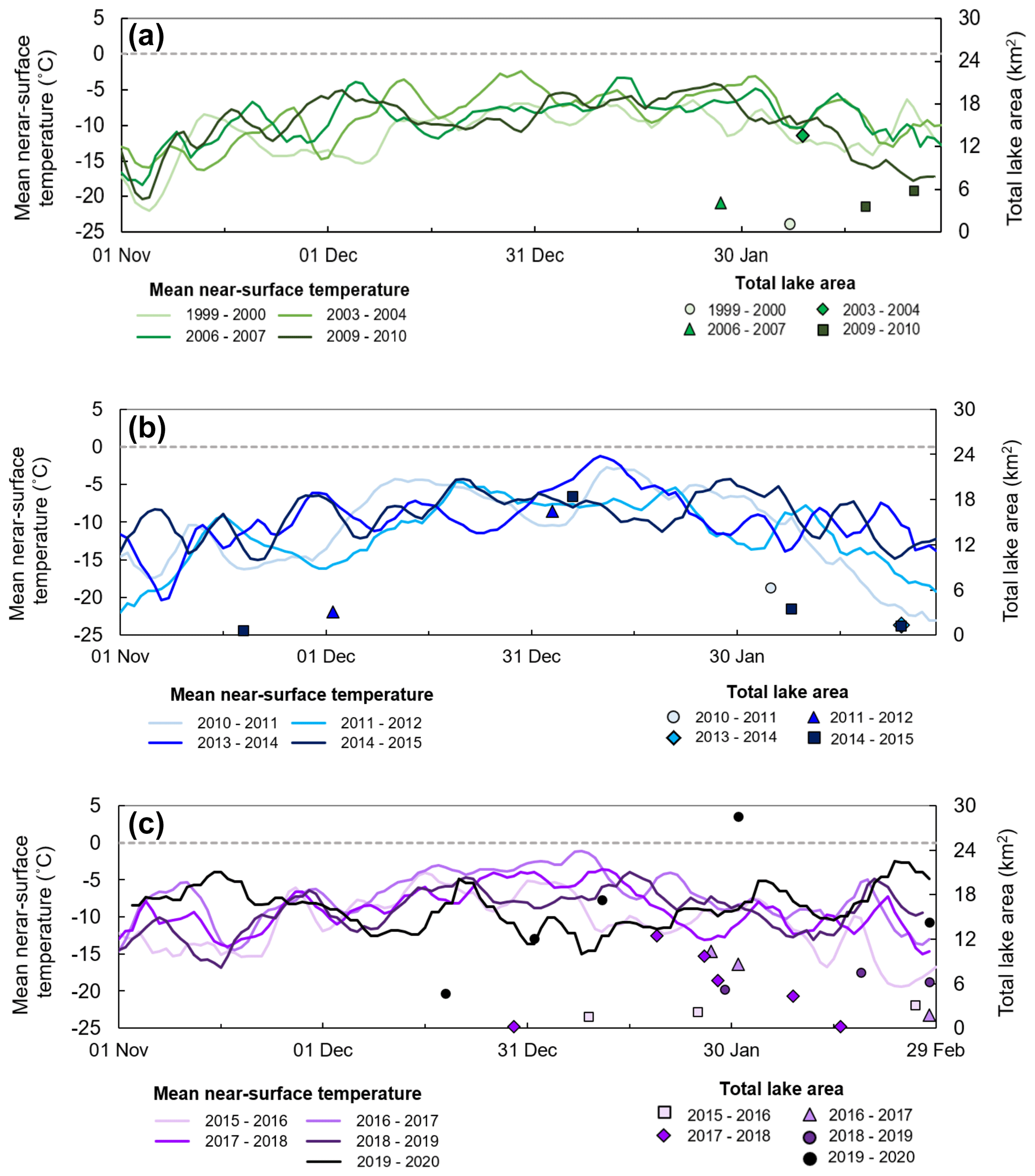
Figure 7Total supraglacial lake area and mean near-surface (2 m) temperature for 1999–2004 (a), 2010–2015 (b) and 2015–2020 (c). Mean near-surface temperature is the mean extracted over the whole Shackleton Ice Shelf (shown as a 5 d moving average).
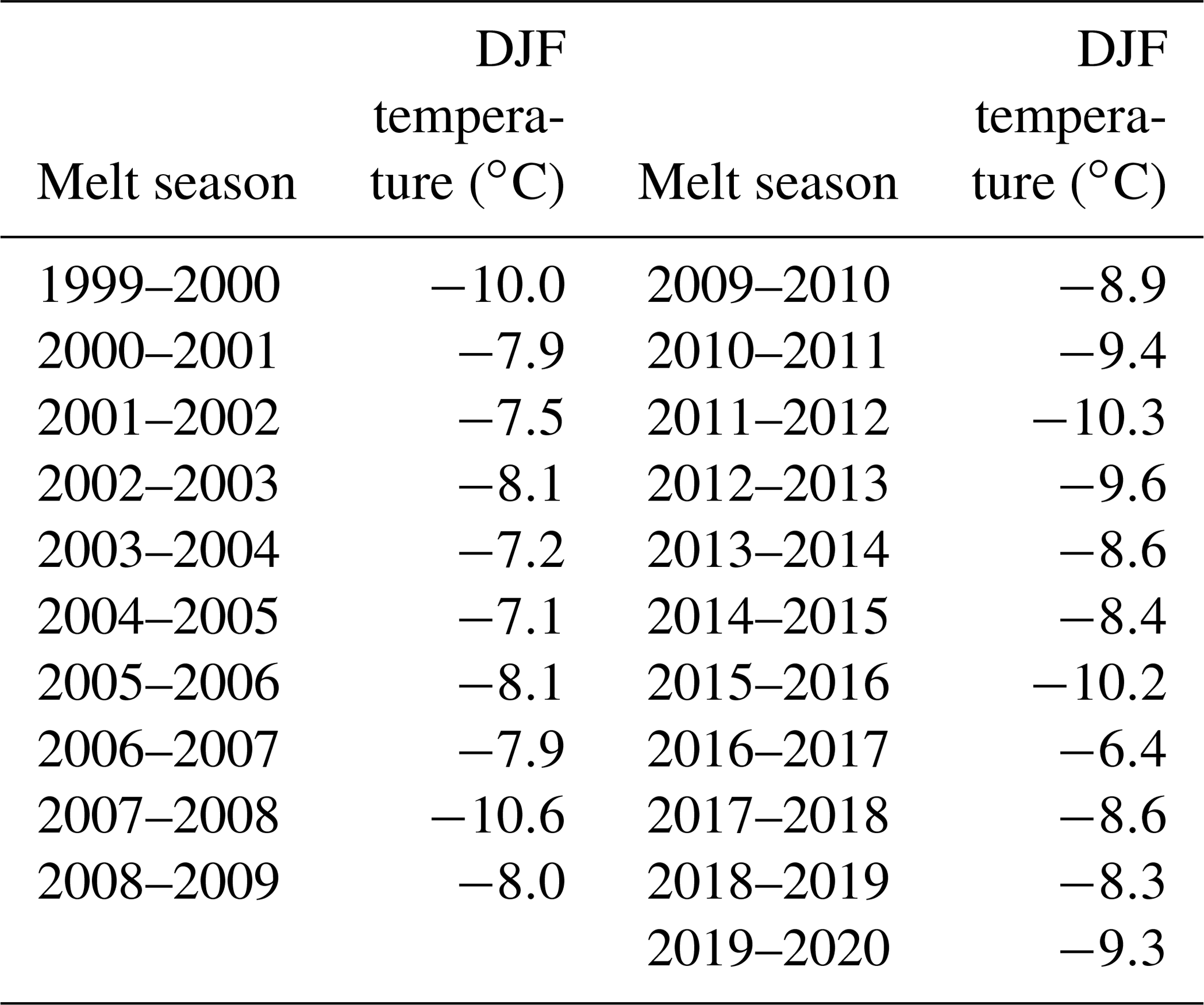
Table 2Average December–January–February (DJF) near-surface temperatures from ERA5 on Shackleton Ice Shelf from 2000 to 2020.
To investigate whether there was a correspondence between peak lake area and volume on the one hand and surface melt rates (which include meltwater available to refreeze in the firn) on the other, we compared our lake dataset to modelled surface melt from RACMO 2.3p1. Multiple large (> 4 mm w.e. d−1) but generally short lived (≤ 1 week) spikes in melt are modelled, separated by periods of little to no surface melt (Fig. 9). A correspondence between peak lake area, volume and surface melt is particularly apparent in 2014, 2015, 2017 and 2018 (Fig. 9). For example, in 2014–2015, total lake area (18.3 km2) and volume (31.5×10⁶ m3) peak 5 d after a large surface melt event (9 mm w.e d−1; Fig. 9b). Similarly, in 2017–2018, total lake area (12.4 km2) and volume (15.2×10⁶ m3) peak 8 d after a spike in surface melt (11 mm w.e d−1; Fig. 9d). Though total lake area and volume may have peaked more rapidly following these modelled surface melt events, temporal gaps in cloud-free imagery prevent us from constraining these timings further. Unfortunately, we have insufficient observations to detect whether a correspondence exists between peak lake area, volume and surface melt in other melt seasons (Fig. S5). We also note that at the time of submission, RACMO2.3p1 data for the 2019–2020 melt season are unavailable, which prevents us from comparing surface melt with total lake area and volume over this period. According to simulations by RACMO 2.3p1 over the whole ice shelf, total lake area is not significantly correlated to minimum firn air content (FAC; r20.01, p=0.56) and mean FAC (r20.009, p=0.63) during the years for which we had lake observations (Fig. 10a–b). However, there is a qualitative correspondence between years of particularly low mean and minimum FAC and years of high melt (2014, 2015 and 2017; Fig. 10c). During these years, mean FAC ranged from 14.5 to 14.59 m and minimum FAC did not exceed 0.31 m.
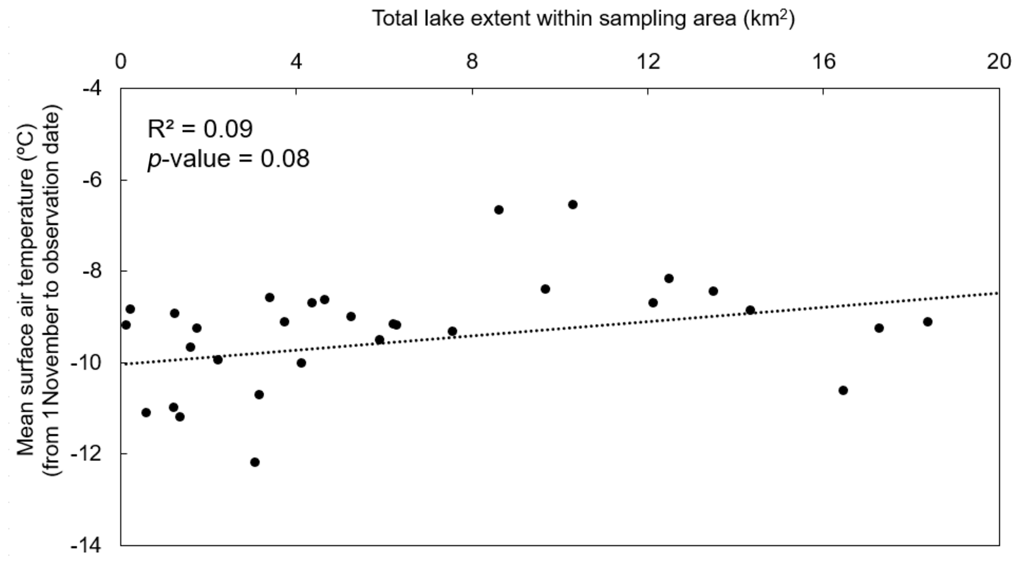
Figure 8Scatter plot of total lake area inside the subset area highlighted in Fig. 1 (green box) and mean surface air temperature from 1 November to the date of each observation.
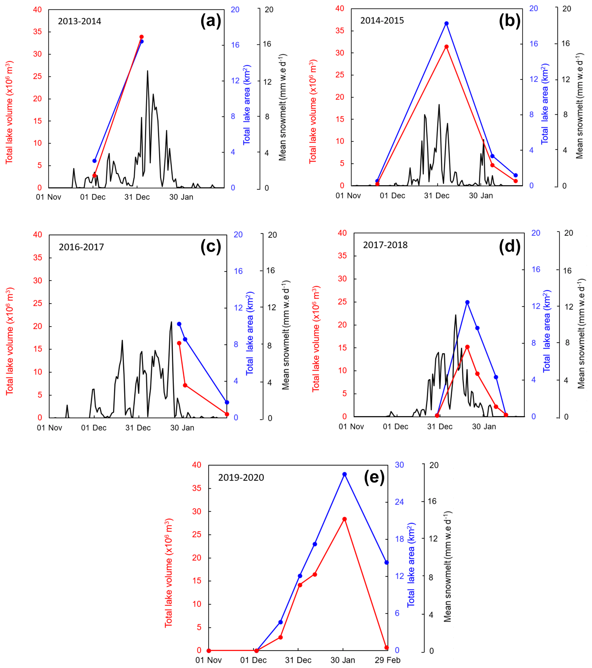
Figure 9Seasonal variations in total lake area, volume and modelled snowmelt on Shackleton Ice Shelf during the melt seasons 2013–2014 (a), 2014–2015 (b), 2016–2017 (c), 2017–2018 (d) and 2019–2020 (e) within the subset area (green box, Fig. 1). Peak total lake area and volume is associated with a spike in snowmelt. Snowmelt rates are mean values over the entire ice shelf.
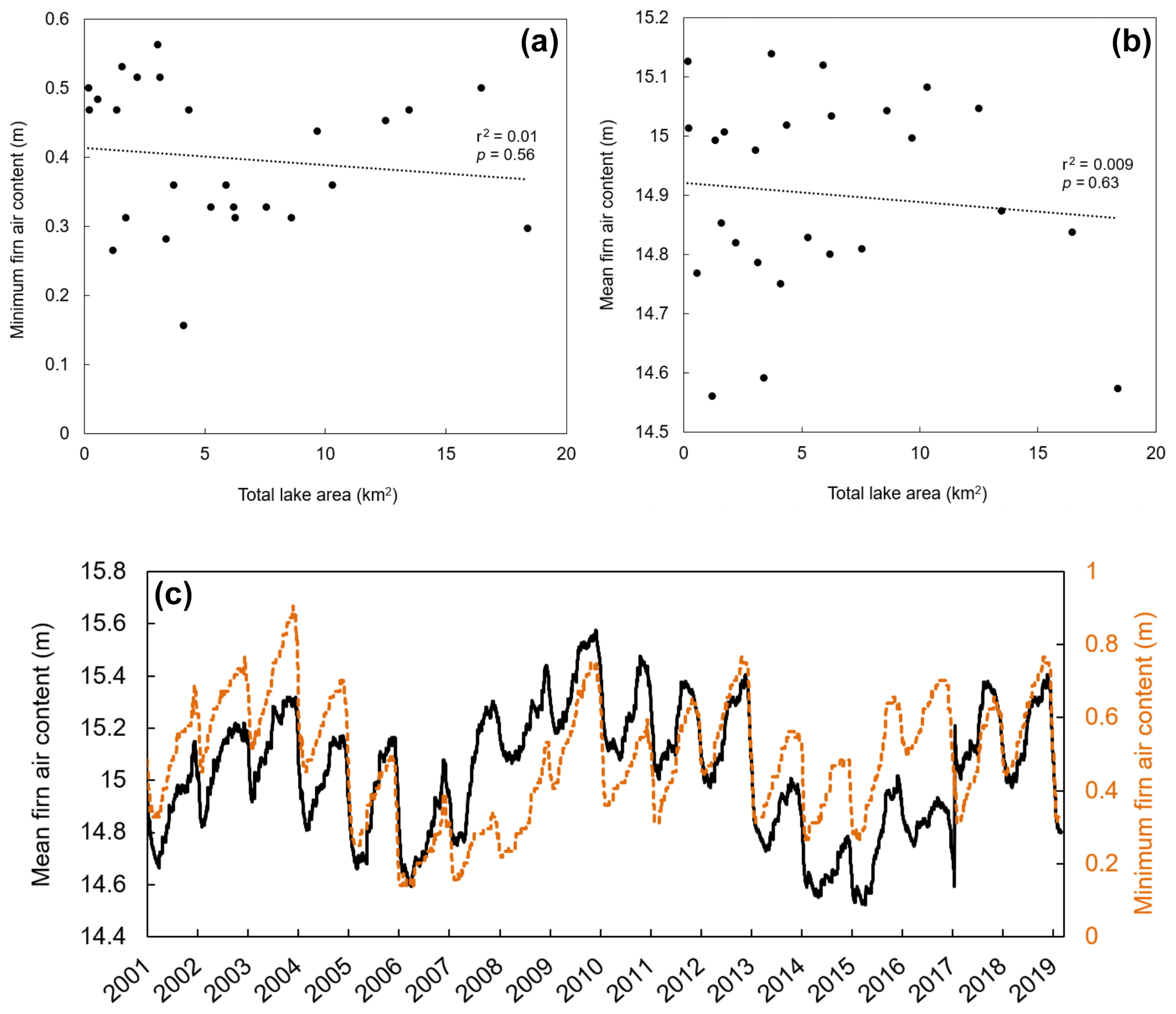
Figure 10(a) Mean firn air content (total integrated pore space, i.e. the thickness of the equivalent air column contained in the firn in metres) over Shackleton Ice Shelf from 2000 to 2019. (b) Scatter plot comparing minimum fir air content and total lake area. (c) Time series comparing mean firn air content, minimum firn air content and total lake area.
5.1 Spatial distribution of SGLs
The clustering of SGLs in the grounding zone of Shackleton Ice Shelf can be explained by localised katabatic-wind-driven feedbacks. Extensive blue-ice areas upstream of the grounding line and adjacent to the Bunger Hills nunataks (Fig. 1) are indicative of persistent snow surface scouring by easterly katabatic winds. These winds descend from the Polar Plateau, generated by large surface slopes (> 20∘), and reach 19 m s−1 in summer (Doran et al., 1996). Surface meltwater production is enhanced as the winds warm adiabatically as they descend to the grounding zone, which lowers humidity and raises near-surface air temperatures (Doran et al., 1996; Lenaerts et al., 2017). The lower albedo of blue-ice areas (∼ 0.5) compared to refrozen snow (∼ 0.7) exerts a positive feedback on surface melting by enhancing solar radiation absorption (Kingslake et al., 2017; Lenaerts et al., 2017; Stokes et al., 2019). SGLs have been associated with strong katabatic-wind-induced scouring of blue-ice areas on several other East Antarctic ice shelves (Bell et al., 2017; Kingslake et al., 2017; Lenaerts et al., 2017; Stokes et al., 2019). This albedo-lowering feedback is locally enhanced by the presence of the Bunger Hills and surrounding nunataks (Fig. 1), whose lower albedo further enhances surface melting and ponding on these portions of the ice shelf. This is a typically localised effect (i.e. within 10 km; Kingslake et al., 2017; Leppäranta et al., 2013; Winther et al., 1996; Stokes et al., 2019).
It is also clear that firn air content (FAC) is an important control on the spatial distribution of SGLs on Shackleton Ice Shelf. Lake clustering near the grounding line means repeated meltwater percolation and refreezing into the snow and firn layers is likely to have formed refrozen ice lenses or superimposed ice zones (Hubbard et al., 2016). The large coalesced lakes we observed in 2014, 2015 and 2020 (e.g. Fig. 2d) are suggestive of the firn layer becoming saturated in this portion of the shelf. Simulations from RACMO 2.3p1 indicate that the FAC may be as low as ≤ 1 m on parts of the ice shelf (Fig. 10a, c). SGLs could therefore become more extensive in the ice shelf grounding zone in future, because saturated firn promotes surface ponding by limiting meltwater percolation and its lateral flow within the firn layer (Alley et al., 2018; Hubbard et al., 2016; Lenaerts et al., 2017). The absence of SGLs further down the ice from the grounding zone can be explained by increased accumulation (snowfall) rates towards the ice shelf calving front which result in a correspondingly higher FAC, meaning surface meltwater can be retained in a deeper snowpack and in firn before it can pond into SGLs (Bell et al., 2017; Stokes et al., 2019). Thus, the clustering of SGLs around the grounding line is suggestive of air-depleted firn, which acts as a primary control on where meltwater can pond on the ice shelf surface.
At a more local scale, lakes on grounded ice upstream of the ice shelf grounding line have a high tendency to reform annually in the same locations (Fig. 2), which we attribute to the glaciological processes controlling SGL formation. Ice surface depressions on grounded ice are translations of subglacial topographic undulations and are therefore fixed in space rather than migrating with ice flow (Echelmeyer et al., 1991; Lampkin and VanderBerg, 2011; Langley et al., 2016). Conversely, lakes on the ice shelf itself are generally shorter-lived because they form in surface depressions that migrate annually with ice flow and are progressively advected towards the ice shelf front, as on other Antarctic ice shelves (Banwell et al., 2014; Bell et al., 2017; Glasser and Gudmundsson, 2012; Luckman et al., 2014; Reynolds and Smith, 1981). We speculate that surface undulations perpendicular to the grounding line (i.e. parallel to ice flow) may form as ice flow converges when it crosses the break in slope and is deflected around the Bunger Hills (Fig. 2c), which could flex and fracture the ice (Banwell et al., 2014; Glasser and Gudmundsson, 2012).
Though lakes on the ice shelf are commonly more transient and appear in different locations each year, some larger lakes on the eastern portion of the ice shelf and on Apfel Glacier have a high tendency to reform annually in the same locations (Fig. 2b and c). This characteristic has not previously been reported, and we suggest this occurs because these lakes are located on very slow moving ice near the grounding line (< 50 m yr−1) where annual ice advection is minimal. Between 2000 and 2020, SGLs on the ice shelf are only slightly shallower than those upstream of the grounding line, as has been recorded on Petermann Glacier in Greenland (Fig. S4a–b; MacDonald et al., 2018). Furthermore, in years with higher meltwater volumes, lakes grew deeper on the ice shelf than on grounded ice (Fig. S4c–d). This is perhaps surprising as slow ice flow produces low-amplitude ice surface topography and shallower depressions, so we would expect grounded lakes to be deeper (Pope et al., 2016). We suggest greater numbers of deeper structural depressions form in the ice shelf grounding zone where there are an extensional flow regime and very low slopes conducive to meltwater ponding (Fig. 3b). Inter-annual lake deepening amplified by lake-bottom ablation could also mean lakes on the ice shelf evolve to be deeper than those on ice upstream of the grounding line (Banwell and MacAyeal, 2015). We do not observe inter-annual deepening of individual lakes in our study.
The spatial distribution of SGLs mapped in this study closely follows predicted meltwater routing pathways derived from a surface DEM, which assumes widespread firn saturation across the ice shelf (Fig. S6). Hydrological routing analysis shows meltwater coalesces from steeper upstream parts of the ice shelf and converges in structurally determined topographic lows, such as flow stripes and crevasses on faster-flowing ice, downstream of ice rises, and in shear margins (Fig. S6). This could have future implications for ice shelf stability, though we note that our routing analysis does not allow for water storage in the firn (Sect. 5.3).
5.2 Seasonal evolution of SGLs
SGLs on Shackleton Ice Shelf exhibit strong intra-seasonal and inter-seasonal variations in area, depth and volume, as do studies on Langhovde Glacier and the Nansen and Amery ice shelves (Bell et al., 2017; Langley et al., 2016; Moussavi et al., 2020). In melt seasons when lakes store larger total volumes of surface meltwater on Shackleton Ice Shelf, lakes are more extensive and some are fed by supraglacial rivers, which are not present in lower-melt years (Figs. 4, 6g–j). Notably, we find a correspondence between short-lived, high-magnitude modelled snowmelt events and peak total lake area and volume during years of high surface meltwater storage (i.e. the melt seasons with maximum lake area, depth and volume: 2013–2014, 2014–2015, 2016–2017 and 2017–2018; Fig. 9). These spikes in modelled snowmelt could represent localised katabatic-wind-induced melt events, similar to föhn-wind-induced melt events on the Antarctic Peninsula modelled by regional climate models (Kuipers Munneke et al., 2018; Tuckett et al., 2019). Föhn wind events have been shown to increase surface melt intensity and control the large interannual temporal and spatial variability in surface melt on the Antarctic Peninsula (Cape et al., 2015; Turton et al., 2020). Although 2019–2020 modelled surface melt data are currently unavailable for us to compare with total lake area and volume, we note that this was an exceptional melt season (Fettweis, 2020) in which we recorded the highest total lake area and volume over the 2000–2020 period (Fig. 9e). Previous work based on meteorological observations from Ekström Ice Shelf, East Antarctica, has suggested that snowmelt–albedo feedbacks exert a key control on melt intensity and duration (Jakobs et al., 2019). Therefore, variations in the strength of this snowmelt–albedo feedback could exert an important control on the amount of melt seasonally available to pond into SGLs on Shackleton Ice Shelf.
Interestingly, the years when total lake area, depth and volume were highest did not always correspond with warmer summer near-surface temperatures (Fig. 7). In particular, mean DJF temperatures during years with the highest surface meltwater storage were actually lower than some years with much less extensive and shallower lakes (Table 2). Furthermore, the weak positive relationship we observe between total SGL area and mean surface air temperature in the preceding part of the melt season (Fig. 8) contrasts with previous studies which show SGLs are highly sensitive to small fluctuations in surface temperature (e.g. Langley et al., 2016). Rather, we suggest that seasonal fluctuations in lake area and volume on this ice shelf are more sensitive to snowmelt intensity associated with katabatic-wind-driven melting, rather than to longer-term patterns of mean near-surface summer temperature. Therefore, intense short-lived melt events appear to determine seasonal variability in SGL extent and volume. This is important because short-lived katabatic events and albedo feedbacks are difficult to resolve in regional climate models such as RACMO, owing to its 27 km resolution (Van Wessem et al., 2018). Although RACMO2.3p1 output is available at a 5.5 km resolution in some regions of Antarctica, it does not yet extend to our study region. This finding underscores the need for finer-resolution regional climate model simulations of surface melt when considering future lake distributions (Arthur et al., 2020a; Stokes et al., 2019). The weak relationship that we observe between SGL extents and near-surface temperature is perhaps unsurprising given the resolution of ERA5 is insufficient to resolve localised mixing and albedo-lowering processes around the ice shelf grounding zone, but our preliminary comparison between SGL development and climate offers some clear hints that short-lived melt events are more important than longer-term seasonal conditions.
Regarding individual lake development, the lakes that we observed to drain englacially within a ≤ 7 d period did so more rapidly than lakes on the Amery Ice Shelf where lakes have drained within 10 d (Moussavi et al., 2020). This is still slower than on the Greenland Ice Sheet, where lakes drain on hourly or daily timescales (e.g. Das et al., 2008; Doyle et al., 2013; Selmes et al., 2013; Stevens et al., 2015; Williamson et al., 2017). We note that the lake drainages we observed could have drained on subdaily timescales comparable to Greenland, but this is not detectable from the temporal resolution of the satellite imagery used in this study. Ice shelf thicknesses in the region where lakes drained englacially (Fig. 6k–l) reach 150–200 m, which is comparable to the ∼ 200 m thickness of Larsen B through which lakes are thought to have drained prior to its collapse (Banwell et al., 2013; MacAyeal and Sergienko, 2013; Scambos et al., 2003). Therefore, lakes could potentially have drained through the full ice shelf thickness via lake bed crevasses. However, because no lakes drained fully, we suggest they are more likely to have drained into the firn and subsequently refrozen.
Most lakes do not drain, instead refreezing at the end of the melt season, which is consistent with the decline in total lake area and volume from late January to late February (Fig. 7) and is common elsewhere in East Antarctica (e.g. Langley et al., 2016; Leppäranta et al., 2013). Once meltwater penetrates the snowpack and reaches a subfreezing firn temperature, it refreezes and raises the surrounding firn temperature by releasing latent heat (Buzzard et al., 2018; Bevan et al., 2018; Jakobs et al., 2019). Meltwater refreezing within the firn produces larger snow grains with a lower albedo, which are more likely to absorb incoming solar radiation and further enhance surface melting (Gardner and Sharp, 2010). Thus, our observations of lakes repeatedly refreezing at the end of each melt season are likely to indicate meltwater storage and refreezing in the ice shelf firn layer near the grounding line.
5.3 Implications for ice shelf stability
Future warming is expected to enhance surface melting and increase surface meltwater production in Antarctica (Bell et al., 2018; Kingslake et al., 2017; Rintoul et al., 2018; Trusel et al., 2015). Increased lake coverage and meltwater storage in future years could cause the ice shelf to flex (Banwell and MacAyeal, 2015; Banwell et al., 2019), which could lead to fracture. Previous work has suggested that FAC can be used to infer shelf stability and likelihood of hydrofracture (Alley et al., 2018; Holland et al., 2011; Lenaerts et al., 2017). We find simulated minimum FAC is close to zero in the grounding zone of Shackleton Ice Shelf, consistent with simulated FAC on the Roi Baudouin (Lenaerts et al., 2017) and pre-collapse Larsen B (Leeson et al., 2020) ice shelves. Therefore, despite limited (< 1 %) lake coverage on the ice shelf at present, its susceptibility to widespread ponding and hydrofracture is likely to gradually increase as FAC is depleted (Alley et al., 2018; Leeson et al., 2020; Lenaerts et al., 2017). Our meltwater routing analysis suggests that the ice shelf could potentially support and route water along surface troughs to the ice shelf edge, similar to active shear-margin rivers present on Nansen Ice Shelf (Fig. S6; Bell et al., 2017), which could partially mitigate the effect of surface meltwater loading (Bell et al., 2017).
This study presents the first quantitative, multiyear study of SGL evolution on East Antarctica's sixth-largest ice shelf. Between the melt seasons of 1999–2000 and 2019–2020, melt seasons were characterised by hundreds of SGLs that were, on average, 0.02 km2 in area and 0.96 m deep and held a mean total meltwater volume of 7.45×10⁶ m3.
We also find the following:
-
Lakes cluster around the grounding line, controlled by localised albedo-lowering feedbacks caused by interactions between katabatic-driven melting, blue ice and exposed bedrock (Kingslake et al., 2017; Lenaerts et al., 2017; Stokes et al., 2019).
-
Lakes on the ice shelf are more transient than those on grounded ice, the latter of which reform annually in the same locations. Some lakes on slow-moving parts of the ice shelf near the grounding line also frequently occupy the same ice surface depressions, which likely results from minimal ice advection in these areas.
-
Lakes begin to form from mid-November, and their total volume, which reached a maximum of 28.4×10⁶ m3 on 31 January 2020, peaks in early–late January each year.
-
SGLs were most extensive and deepest and formed at the highest recorded elevation (527 m) in 2014, 2015, 2017, 2018 and 2020. At the peak of these melt seasons, parts of the ice shelf grounding zone became saturated with meltwater which coalesced into large lakes, and lakes were fed by supraglacial rivers.
-
Short-lived high-magnitude snowmelt events correspond with peak total lake area and volume during these years of high surface meltwater storage. Seasonal variability in lake extents is more sensitive to the intensity of individual melt events rather than to mean near-surface summer temperatures, which we suggest is driven by localised katabatic-wind-induced melting.
Our findings may be used to inform the boundary conditions and validation of supraglacial hydrology models, for example to validate estimates of lake distributions and to constrain volume-dependent lake drainage thresholds. In particular, our data quantify the meltwater volumes being stored on the ice shelf surface, highlighting the importance of increased meltwater storage within SGLs during melt seasons experiencing intense, short-lived melt events. An improved understanding of East Antarctica's present surface hydrology has significance for constraining future dynamic change in the ice sheet and its contribution to sea-level rise.
The supraglacial lake extents and depths discussed in this paper are available at https://doi.org/10.5285/649bbe03-8109-45be-92e5-bcef44a4703a (Arthur et al., 2020a). Sentinel imagery is available from the Copernicus Open Access Hub (https://scihub.copernicus.eu, last access: February 2020; Copernicus Open Access Hub, 2020), and Landsat scenes are available from United States Geological Survey EarthExplorer (https://earthexplorer.usgs.gov/, last access: February 2020; EarthExplorer, 2020). ERA5 reanalysis surface temperature is available from the Copernicus Climate Change Service Climate Date Store (https://cds.climate.copernicus.eu/, last access: March 2020).
The supplement related to this article is available online at: https://doi.org/10.5194/tc-14-4103-2020-supplement.
JFA, CRS and SSJ designed the initial study. JFA undertook the data collection and conducted the analysis, with guidance from all authors. JFA led the manuscript writing, with input from all authors.
The authors declare that they have no conflict of interest.
JFA was funded by the IAPETUS Natural Environment Research Council (NERC) Doctoral Training Partnership (grant number NE/L002590/1). Chris R. Stokes and Stewart S. R. Jamieson were supported by NERC grant NE/R000824/1. We acknowledge RACMO data from Michiel Roland van den Broeke, the Norwegian Polar Institute's Quantarctica package and Copernicus Climate Change Service information (ERA5 reanalysis). Jennifer F. Arthur acknowledges Bertie Miles for helpful discussions during this work. We would like to thank Jan Lenaerts and the anonymous reviewer for providing constructive comments which led to improvement of this paper and the editor (Stef Lhermitte) for handling the manuscript.
This research has been supported by the Natural Environment Research Council (grant nos. NE/L002590/1 and NE/R000824/1).
This paper was edited by Stef Lhermitte and reviewed by Jan Lenaerts and one anonymous referee.
Alley, K. E., Scambos, T. A., Miller, J. Z., Long, D. G., and MacFerrin, M.: Quantifying vulnerability of Antarctic ice shelves to hydrofracture using microwave scattering properties, Remote. Sens. Environ., 210, https://doi.org/10.1016/j.rse.2018.03.025, 2018.
Arthur, J. F, Stokes, C. R., Jamieson, S. S. R, Carr, J. R, and Leeson, A. A.: Observations of supraglacial lakes on Shackleton Ice Shelf, East Antarctica from 1974 to 2020, Polar Data Centre, Nat. Environ. Res. Council, UKGB/NERC/BAS/PDC/01376, https://doi.org/10.5285/649bbe03-8109-45be-92e5-bcef44a4703a, 2020a.
Arthur, J. F., Stokes, C. R., Jamieson, S. S. R., Carr, J. R., and Leeson, A. A.: Recent understanding of Antarctic supraglacial lakes using satellite remote sensing, Prog. Phys. Geogr., 1–32, 2020b.
Banwell, A. F., MacAyeal, D. R., and Sergienko, O. V.: Breakup of the Larsen B Ice Shelf triggered by chain reaction drainage of supraglacial lakes, Geophys. Res. Lett, 40, 5872–5876, https://doi.org/10.1002/2013GL057694, 2013.
Banwell, A. F. and MacAyeal, D. R.: Ice-shelf fracture due to viscoelastic flexure stress induced by fill/drain cycles of supraglacial lakes, Antarct. Sci, 27, 587–597, https://doi.org/10.1017/S0954102015000292, 2015.
Banwell, A. F., Caballero, M., Arnold, N. S., Glasser, N. F., Cathles, L. M., and MacAyeal, D. R.: Supraglacial lakes on the Larsen B ice shelf, Antarctica, and at Paakitsoq, West Greenland: A comparative study, Ann. Glaciol, 55, 1–8, https://doi.org/10.3189/2014AoG66A049, 2014.
Banwell, A. F., Willis, I. C., Macdonald, G. J., Goodsell, B., and MacAyeal, D. R.: Direct measurements of ice-shelf flexure caused by surface meltwater ponding and drainage, Nat. Commun., 10, 730, https://doi.org/10.1038/s41467-019-08522-5, 2019.
Bell, R. E., Chu, W., Kingslake, J., Das, I., Tedesco, M., Tinto, K. J., Zappa, C. J., Frezzotti, M., Boghosian, A., and Sang Lee, W.: Antarctic ice shelf potentially stabilized by export of meltwater in surface river, Nature, 544, 344–348, https://doi.org/10.1038/nature22048, 2017.
Bell, R. E., Banwell, A. F., Trusel, L. D., and Kingslake, J.: Antarctic surface hydrology and impacts on ice-sheet mass balance, Nat. Clim. Change, 8, 1044–1052, https://doi.org/10.1038/s41558-018-0326-3, 2018.
Bevan, S. L., Luckman, A. J., Kuipers Munneke, P., Hubbard, B., Kulessa, B., and Ashmore, D. W.: Decline in Surface Melt Duration on Larsen C Ice Shelf Revealed by The Advanced Scatterometer (ASCAT), Earth Space Sci., 5, https://doi.org/10.1029/2018EA000421, 2018.
Bindschadler, R. A., Vornberger, P., Fleming, A., Fox, A.D., Mullins, J., Binnie, D., Paulsen, S., Granneman, B., and Gorodetzky, D.: The Landsat image mosaic of Antarctica, Remote Sens. Environ., 112, 4214–4226, https://doi.org/10.1016/j.rse.2008.07.006, 2008.
Box, J. E. and Ski, K.: Remote sounding of Greenland supraglacial melt lakes: Implications for subglacial hydraulics, J. Glaciol., 53, 257–265, https://doi.org/10.3189/172756507782202883, 2007.
Burton-Johnson, A., Black, M., Fretwell, P. T., and Kaluza-Gilbert, J.: An automated methodology for differentiating rock from snow, clouds and sea in Antarctica from Landsat 8 imagery: a new rock outcrop map and area estimation for the entire Antarctic continent, The Cryosphere, 10, 1665–1677, https://doi.org/10.5194/tc-10-1665-2016, 2016.
Buzzard, S. C., Feltham, D. L., and Flocco, D.: A Mathematical Model of Melt Lake Development on an Ice Shelf, J. Adv. Model. Earth Syst., 10, 262–283, https://doi.org/10.1002/2017MS001155, 2018.
Cape, M. R., Vernet, M., Skvarca, P., Marinsek, S., Scambos, T., and Domack, E.: Foehn winds link climate‐driven warming to ice shelf evolution in Antarctica, J. Geophys. Res., 120, 11037–11507, https://doi.org/10.1002/2015JD023465, 2015.
Copernicus Open Access Hub, European Space Agency, available at: https://scihub.copernicus.eu, last access: February 2020.
Das, S. B., Joughin, I., Behn, M. D., Howat, I. M., King, M. A., Lizarralde, D., and Bhatia, M. P.: Fracture propagation to the base of the Greenland ice sheet during supraglacial lake drainage, Science, 320, 778–781, https://doi.org/10.1126/science.1153360, 2008.
Dell, R., Arnold, N., Willis, I., Banwell, A., Williamson, A., Pritchard, H., and Orr, A.: Lateral meltwater transfer across an Antarctic ice shelf, The Cryosphere, 14, 2313–2330, https://doi.org/10.5194/tc-14-2313-2020, 2020.
DLR: Grounding line for Denman Glacier, derived from ERS-1/2 and Copernicus Sentinel-1 data acquired in 1996, 2015 and 2017, Antarctic Ice Sheet CCI [release date 2018-07-02, v1.0], 2018.
Doran, P. T., McKay, C. P., Meyer, M. A., Andersen, D. T., Wharton, R. A., and Hastings, J. T.: Climatology and implications for perennial lake ice occurrence at Bunger Hills Oasis, East Antarctica, Antarct. Sci., 8, 289–296, https://doi.org/10.1017/s0954102096000429, 1996.
Doyle, S. H., Hubbard, A. L., Dow, C. F., Jones, G. A., Fitzpatrick, A., Gusmeroli, A., Kulessa, B., Lindback, K., Pettersson, R., and Box, J. E.: Ice tectonic deformation during the rapid in situ drainage of a supraglacial lake on the Greenland Ice Sheet, The Cryosphere, 7, 129–140, https://doi.org/10.5194/tc-7-129-2013, 2013.
EarthExplorer, United States Geological Survey, available at: https://earthexplorer.usgs.gov/, last access: February 2020.
Echelmeyer, K., Clarke, T. S., and Harrison, W. D.: Surficial glaciology of Jakobshavns Isbræ, West Greenland: Part I. Surface morphology, J. Glaciol., 37, 368–382, https://doi.org/10.3189/S0022143000005803, 1991.
Fettweis, X.: 5-day forecast of the 2019–2020 Antarctic ice sheet SMB simulated by MARv3.11 forced by GFS, available at: https://climato.uliege.be/cms/c_5652669/fr/climato-antarctica, last access: 17 April 2020.
Flament, T. and Rémy, F.: Dynamic thinning of Antarctic glaciers from along-track repeat radar altimetry, J. Glaciol., 58, 830–840, https://doi.org/10.3189/2012JoG11J118, 2012.
Fretwell, P., Pritchard, H. D., Vaughan, D. G., Bamber, J. L., Barrand, N. E., Bell, R., Bianchi, C., Bingham, R. G., Blankenship, D. D., Casassa, G., Catania, G., Callens, D., Conway, H., Cook, A. J., Corr, H. F. J., Damaske, D., Damm, V., Ferraccioli, F., Forsberg, R., Fujita, S., Gim, Y., Gogineni, P., Griggs, J. A., Hindmarsh, R. C. A., Holmlund, P., Holt, J. W., Jacobel, R. W., Jenkins, A., Jokat, W., Jordan, T., King, E. C., Kohler, J., Krabill, W., Riger-Kusk, M., Langley, K. A., Leitchenkov, G., Leuschen, C., Luyendyk, B. P., Matsuoka, K., Mouginot, J., Nitsche, F. O., Nogi, Y., Nost, O. A., Popov, S. V., Rignot, E., Rippin, D. M., Rivera, A., Roberts, J., Ross, N., Siegert, M. J., Smith, A. M., Steinhage, D., Studinger, M., Sun, B., Tinto, B. K., Welch, B. C., Wilson, D., Young, D. A., Xiangbin, C., and Zirizzotti, A.: Bedmap2: improved ice bed, surface and thickness datasets for Antarctica, The Cryosphere, 7, 375–393, https://doi.org/10.5194/tc-7-375-2013, 2013.
Fürst, J. J., Durand, G., Gillet-Chaulet, F., Tavard, L., Rankl, M., Braun, M., and Gagliardini, O.: The safety band of Antarctic ice shelves, Nat. Clim. Change, 6, 479–482, https://doi.org/10.1038/nclimate2912, 2016.
Gardner, A. S. and Sharp, M. J.: A review of snow and ice albedo and the development of a new physically based broadband albedo parameterization, J. Geophys. Res.-Earth Surf., 115, F1, https://doi.org/10.1029/2009JF001444, 2010.
Gillespie, A. R., Kahle, A. B., and Walker, R. E.: Color enhancement of highly correlated images. II. Channel ratio and “chromaticity” transformation techniques, Remote Sens. Environ., 22, 343–365, https://doi.org/10.1016/0034-4257(87)90088-5, 1987.
Glasser, N. and Scambos, T.: A structural glaciological analysis of the 2002 Larsen B ice-shelf collapse, J. Glaciol., 54, 3–16, https://doi.org/10.1136/archdischild-2015-309290, 2008.
Glasser, N. F. and Gudmundsson, G. H.: Longitudinal surface structures (flowstripes) on Antarctic glaciers, The Cryosphere, 6, 383–391, https://doi.org/10.5194/tc-6-383-2012, 2012.
Glasser, N. F., Holt, T., Fleming, E., and Stevenson, C.: Ice shelf history determined from deformation styles in surface debris, Ant. Sci., 26, 661–673, https://doi.org/10.1017/S0954102014000376, 2014.
Holland, P. R., Corr, H. F. J., Pritchard, H. D., Vaughan, D. G., Arthern, R. J., Jenkins, A., and Tedesco, M.: The air content of Larsen Ice Shelf, Geophys. Res. Lett., 38, 1–6, https://doi.org/10.1029/2011GL047245, 2011.
Hubbard, B., Luckman, A., Ashmore, D., Bevan, S., Kulessa, B., Kuipers, Munneke, P., Philippe, M., Jansen, D., Booth, A., Sevestre, H., Tison, J., O'Leary, M., and Rutt, I.: Massive subsurface ice formed by refreezing of ice-shelf melt ponds, Nat. Comms., 7, 11897, https://doi.org/10.1038/ncomms11897, 2016.
Jakobs, C. L., Reijmer, C. H., Kuipers Munneke, P., König-Langlo, G., and van den Broeke, M. R.: Quantifying the snowmelt-albedo feedback at Neumayer Station, East Antarctica, The Cryosphere, 13, 1473–1485, https://doi.org/10.5194/tc-13-1473-2019, 2019.
Kingslake, J., Ng, F., and Sole, A.: Modelling channelized surface drainage of supraglacial lakes, J. Glaciol., 61, 185–199, https://doi.org/10.3189/2015JoG14J158, 2015.
Kingslake, J., Ely, J. C., Das, I., and Bell, R. E.: Widespread movement of meltwater onto and across Antarctic ice shelves, Nature, 544, 349–352, https://doi.org/10.1038/nature22049, 2017.
Konrad, H., Shepherd, A., Gilbert, L., Hogg, A. E., McMillan, M., Muir, A., and Slater, T.: Net retreat of Antarctic glacier grounding lines, Nat. Geosci., 11, 258–262, https://doi.org/10.1038/s41561-018-0082-z, 2018.
Kuipers Munneke, P., Luckman, A. J., Bevan, S. L., Smeets, C. J. P. P., Gilbert, E., van den Broeke, M. R., Wang, W., Zender, C., Hubbard, B., Ashmore, D., Orr, A., King, J. C., and Kulessa, B.: Intense Winter surface melting on an Antarctic Ice Shelf, Geophys. Res. Lett., 45, 7615–7623, https://doi.org/10.1029/2018GL077899, 2018.
Lampkin, D. J. and VanderBerg, J.: A preliminary investigation of the influence of basal and surface topography on supraglacial lake distribution near Jakobshavn Isbrae, western Greenland, Hydrol. Process., 25, 3347–3355, https://doi.org/10.1002/hyp.8170, 2011.
Langley, E. S., Leeson, A. A., Stokes, C. R., and Jamieson, S. S. R.: Seasonal evolution of supraglacial lakes on an East Antarctic outlet glacier, Geophys. Res. Lett., 43, 8563–8571, https://doi.org/10.1002/2016GL069511, 2016.
Leeson, A. A., Shepherd, A., Palmer, S., Sundal, A., and Fettweis, X.: Simulating the growth of supraglacial lakes at the western margin of the Greenland ice sheet, The Cryosphere, 6, 1077–1086, https://doi.org/10.5194/tc-6-1077-2012, 2012.
Leeson, A. A., Forster, E., Rice, A., Gourmelen, N., and van Wessem, J. M.: Evolution of supraglacial lakes on the Larsen B ice shelf in the decades before it collapsed, Geophys. Res. Lett., 47, 1–3, https://doi.org/10.1029/2019GL085591, 2020.
Lenaerts, J. T. M., Lhermitte, S., Drews, R., Lightenberg, S. R. M., Berger, S., Helm, V., Smeets, C. J. P. P., van den Broeke, M. R., van de Ber, W. J., van Meijgaard, E., Eijkelboom, M., Eisen, O., and Pattyn, F.: Meltwater produced by wind-albedo interaction stored in an East Antarctic ice shelf, Nat. Clim. Change, 7, 58–62, https://doi.org/10.1038/nclimate3180, 2017.
Leppäranta, M., Järvinen, O., and Mattila, O. P.: Structure and life cycle of supraglacial lakes in Dronning Maud Land, Antarct. Sci., 25, 457–467, https://doi.org/10.1017/S0954102012001009, 2013.
Liang, Q. I., Zhou, C., Howat, I. M., Jeong, S., Liu, R., and Chen, Y.: Ice flow variations at Polar Record Glacier, East Antarctica, J. Glaciol., 65, 279–287, https://doi.org/10.1017/jog.2019.6, 2019.
Luckman, A., Elvidge, A., Jansen, D., Kulessa, B., Kuipers Munneke, P., King, J., and Barrand, N. E.: Surface melt and ponding on Larsen C Ice Shelf and the impact of föhn winds. Antarc. Sci., 26, 625–635, https://doi.org/10.1017/S0954102014000339, 2014.
Lüthje, M., Feltham, D. L., Taylor, P. D., and Worster, M. G.: Modeling the summertime evolution of sea ice melt ponds. J. Geophys. Res., 111, C02001, https://doi.org/10.1029/2004JC002818, 2006.
Macayeal, D. R. and Sergienko, O. V.: The flexural dynamics of melting ice shelves, Ann. Glaciol., 54, 1–10, https://doi.org/10.3189/2013AoG63A256, 2013.
MacDonald, G. J., Banwell, A. F., and MacAyeal, D. R.: Seasonal evolution of supraglacial lakes on a floating ice tongue, Petermann Glacier, Greenland, Ann. Glaciol., 59, 56–65, https://doi.org/10.1017/aog.2018.9, 2018.
MacDonald, G. J., Popović, P., and Mayer, D. P.: Formation of sea ice ponds from ice-shelf runoff, adjacent to the McMurdo Ice Shelf, Antarctica, Ann. Glaciol., 1–5, https://doi.org/10.1017/aog.2020.9, 2020.
Moran, M. S., Jackson, R. D., Slater, P. N., and Teillet, P. M.: Evaluation of simplified procedures for retrieval of land surface reflectance factors from satellite sensor output, Remote Sens. Environ., 41, 169–184, https://doi.org/10.1016/0034-4257(92)90076-V, 1992.
Morlighem, M., Rignot, E., Binder, T., Blankenship, D., Drews, R., Eagles, G., Eisen, O., Ferraccioli, F., Forsberg, R., Fretwell, P., Goel, V., Greenbaum, J. S., Gudmundsson, H., Guo, J., Helm, V., Hofstede, C., Howat, I., Humbert, A., Jokat, W., Karlsson, N. B., Lee, W. S., Matsuoka, K., Millan, R., Mouginot, J., Paden, J., Pattyn, F., Roberts, J., Rosier, S., Ruppel, A., Seroussi, E., Smith, E. C., Steinhage, D., Sun, B., van den Broeke, M. R., van Ommen, T. D., van Wessem, M., and Young, D. A.: Deep glacial troughs and stabilizing ridges unveiled beneath the margins of the Antarctic ice sheet, Nat. Geosci., 13, 132–137, https://doi.org/10.1038/s41561-019-0510-8, 2019.
Moussavi, M. S., Pope, A., Halberstadt, A. R. W., Trusel, L. D., Cioffi, L., and Abdalati, W.: Antarctic supraglacial lake detection using Landsat 8 and Sentinel-2 imagery: towards continental generation of lake volumes, Remote Sens., 12, 134, https://doi.org/10.3390/rs12010134, 2020.
Philpot, W. D.: Bathymetric mapping with passive multispectral imagery, Appl. Opt., 28, 1569–1577, https://doi.org/10.1364/ao.28.001569, 1989.
Pope, A.: Reproducibly estimating and evaluating supraglacial lake depth with Landsat 8 and other multispectral sensors, Earth Space Sci., 3, 176–188, https://doi.org/10.1002/2015EA000125, 2016.
Pope, A., Scambos, T. A., Moussavi, M., Tedesco, M., Willis, M., Shean, D., and Grigsby, S.: Estimating supraglacial lake depth in West Greenland using Landsat 8 and comparison with other multispectral methods, The Cryosphere, 10, 15–27, https://doi.org/10.5194/tc-10-15-2016, 2016.
Pope, R. M. and Fry, E. S.: Absorption spectrum (380–700 nm) of pure water. II. Integrating cavity measurements, Appl. Opt., 36, 8710–8723, https://doi.org/10.1364/AO.36.008710, 1987.
Pritchard, H. D., Ligtenberg, S. R. M., Fricker, H. A., Vaughan, D. G., van den Broeke, M. R., and Padman, L.: Antarctic ice-sheet loss driven by basal melting of ice shelves, Nature, 484, 502–505, https://doi.org/10.1038/nature10968, 2012.
Reynolds, R. W. and Smith, T. M.: Lakes on George VI Ice Shelf, Polar Rec., 20, 425–432, https://doi.org/10.1017/S0032247400003636, 1981.
Rignot, E., Jacobs, S., Mouginot, J., and Scheuchl, B.: Ice-shelf melting around Antarctica, Science, 341, 266–270, https://doi.org/10.1126/science.1235798, 2013.
Rignot, E., Mouginot, J., and Scheuchl, B.: MEaSUREs Antarctic Grounding Line from Differential Satellite Radar Interferometry, Version 2. Boulder, Colorado USA, NASA National Snow and Ice Data Center Distributed Active Archive Center, https://doi.org/https://doi.org/10.5067/IKBWW4RYHF1Q, 2016.
Rignot, E., Mouginot, J., and Scheuchl, B.: MEaSUREs InSAR-Based Antarctica Ice Velocity Map, Version 2, Boulder, Colorado USA, NASA National Snow and Ice Data Center Distributed Active Archive Center, https://doi.org/10.5067/D7GK8F5J8M8R, 2017.
Rignot, E., Mouginot, J., Scheuchl, B., van den Broeke, M., van Wessem, M. J., and Morlighem, M.: Four decades of Antarctic Ice Sheet mass balance from 1979–2017, P. Natl. Acad. Sci., 116, 1095–1103, https://doi.org/10.1073/pnas.1812883116, 2019.
Rintoul, S. R., Chown, S. L., DeConto, R. M., England, M. H., Fricker, H. A., Masson-Delmotte, V., Naish, T. R., Siegert, M. J., and Xavier, J. C.: Choosing the future of Antarctica, Nature, 558, 233–241, https://doi.org/10.1038/s41586-018-0173-4, 2018.
Robel, A. and Banwell, A. F.: A speed limit on ice shelf collapse through hydrofracture, Geophys. Res. Lett., 46, 12092–12100, https://doi.org/10.1029/2019GL084397, 2019.
Roberts, J. L., Warner, R. C., Young, D., Wright, A., van Ommen, T. D., Blankenship, D. D., Siegert, M., Young, N. W., Tabacco, I. E., Forieri, A., Passerini, A., Zirizzotti, A., and Frezzotti, M.: Refined broad-scale sub-glacial morphology of Aurora Subglacial Basin, East Antarctica derived by an ice-dynamics-based interpolation scheme, The Cryosphere, 5, 551–560, https://doi.org/10.5194/tc-5-551-2011, 2011.
Scambos, T. A., Hulbe, C. L, Fahnestock, M. A, and Bohlander, J.: The Link Between Climate Warming and Break-Up of Ice Shelves in the Antarctic Peninsula, J. Glaciol., 46, 516–530, 2000.
Scambos, T., Hulbe, C., and Fahnestock, M.: Climate-induced Ice Shelf Disintegration in the Antarctic Peninsula, Ant. Pen. Clim. Var., Hist Paleo. Persp., 79, 335–347, https://doi.org/10.1029/AR079p0079, 2003.
Scambos, T., Fricker, H. A., Liu, C., Bohlander, J., Fastook, J., Sargent, A., Massom, R., and Wu, A.: Ice shelf disintegration by plate bending and hydro-fracture: Satellite observations and model results of the 2008 Wilkins ice shelf break-ups, Earth Planet. Sci. Lett., 280, 51–60, https://doi.org/10.1016/j.epsl.2008.12.027, 2009.
Selmes, N., Murray, T., and James, T. D.: Characterizing supraglacial lake drainage and freezing on the Greenland Ice Sheet, The Cryosphere Discuss., 7, 475–505, https://doi.org/10.5194/tcd-7-475-2013, 2013.
Sneed, W. A. and Hamilton, G. S.: Evolution of melt pond volume on the surface of the Greenland Ice Sheet. Geophys. Res. Lett., 34, L03501, https://doi.org/10.1029/2006GL028697, 2007.
Stephenson, S. N. and Zwally, H. J.: Ice-shelf topography and structure determined using satellite-radar altimetry and Landsat imagery, Ann. Glaciol., 12, 162–169, 1988.
Stevens, L. A., Behn, M. D., McGuire, J. J., Das, S. B., Joughin, I., Herring, T., Shean, D. E., and King, M. A.: Greenland supraglacial lake drainages triggered by hydrologically induced basal slip, Nature, 522, 73–76, https://doi.org/10.1038/nature14480, 2015.
Stokes, C. R., Sanderson, J. E., Miles, B. W., Jamieson, S. S. R., and Leeson, A. A.: Widespread development of supraglacial lakes around the margin of the East Antarctic Ice Sheet, Sci. Rep., 9, 13823, https://doi.org/10.1038/s41598-019-50343-5, 2019.
Tarboton, D. G.: A New Method for Determination of Flow Directions and Upslope in Grid Elevation Models, Water Resour. Res., 33, 309–319, https://doi.org/10.1029/96WR03137, 1997.
Tedesco, M., Lüthje, M., Steffen, K., Steiner, N., Fettweis, X., Willis, I., Bayou, N., and Banwell, A.: Measurement and modeling of ablation of the bottom of supraglacial lakes in western Greenland, Geophys. Res. Lett., 39, L02502, https://doi.org/10.1029/2011GL049882, 2012.
Trusel, L. D., Frey, K. E., Das, S. B., Kuipers Munneke, P., and van den Broeke, M. R.: Satellite-based estimates of Antarctic surface meltwater fluxes, Geophys. Res. Lett., 40, 6148–6153, https://doi.org/10.1002/2013GL058138, 2013.
Trusel, L. D., Frey, K. E., Das, S. B., Karnauskas, K. B., Kuipers Munneke, P. K., van Meijgaard, E., and van den Broeke, M. R.: Divergent trajectories of Antarctic surface melt under two twenty-first-century climate scenarios, Nat. Geosci., 8, 927–932, https://doi.org/10.1038/ngeo2563, 2015.
Tuckett, P. A., Ely, J. C., Sole, A. J., Livingstone, S. J., Davison, B. J., van Wessem, J. M., and Howard, J.: Rapid accelerations of Antarctic Peninsula outlet glaciers driven by surface melt, Nat. Commun., 10, 1–8, https://doi.org/10.1038/s41467-019-12039-2, 2019.
Turton, J. V., Kirchgaessner, A., Ross, A. N., King, J. C., and Kuipers Munneke, P.: The influence of föhn winds on annual and seasonal surface melt on the Larsen C Ice Shelf, Antarctica, The Cryosphere Discuss., https://doi.org/10.5194/tc-2020-72, in review, 2020.
van Wessem, J. M., van de Berg, W. J., Noël, B. P. Y., van Meijgaard, E., Amory, C., Birnbaum, G., Jakobs, C. L., Krüger, K., Lenaerts, J. T. M., Lhermitte, S., Ligtenberg, S. R. M., Medley, B., Reijmer, C. H., van Tricht, K., Trusel, L. D., van Ulft, L. H., Wouters, B., Wuite, J., and van den Broeke, M. R.: Modelling the climate and surface mass balance of polar ice sheets using RACMO2 – Part 2: Antarctica (1979–2016), The Cryosphere, 12, 1479–1498, https://doi.org/10.5194/tc-12-1479-2018, 2018.
Wearing, M. G., Hindmarsh, R. C. A., and Worster, M. G.: Assessment of ice flow dynamics in the zone close to the calving front of Antarctic ice shelves, J. Glaciol., 61, 1194–1206, https://doi.org/10.3189/2015JoG15J116, 2015.
Williamson, A. G., Arnold, N. S., Banwell, A. F., and Willis, I. C.: A Fully Automated Supraglacial lake area and volume Tracking (“FAST”) algorithm: Development and application using MODIS imagery of West Greenland, Remote Sens. Environn., 196, 113–133, https://doi.org/10.1016/j.rse.2017.04.032, 2017.
Willis, I. C., Pope, E. L., Leysinger Vieli, G. J. M. C., Arnold, N. S., and Long, S.: Drainage networks, lakes and water fluxes beneath the Antarctic ice sheet, Ann. Glaciol., 57, 96–108, https://doi.org/10.1017/aog.2016.15, 2016.
Winther, J., Elvehøy, H., Bøggild, C. E., Sand, K., and Liston, G.: Melting, runoff and the formation of frozen lakes in a mixed snow and blue-ice field in Dronning Maud Land, Antarctica, J. Glaciol., 42, 271–278, https://doi.org/10.3189/S0022143000004135, 1996.
Yang, K. and Smith, L. C.: Supraglacial streams on the Greenland ice sheet delineated from combined spectral-shape information in high-resolution satellite imagery, IEEE Geosci. Remote Sens. Lett., 10, 801–805, https://doi.org/10.1109/LGRS.2012.2224316, 2013.
Zheng, L. and Zhou, C.: Comparisons of snowmelt detected by microwave sensors on the Shackleton Ice Shelf, East Antarctica, Int. J. Remote Sens., 41, 1338–1348, https://doi.org/10.1080/01431161.2019.1666316, 2019.
The requested paper has a corresponding corrigendum published. Please read the corrigendum first before downloading the article.
- Article
(20251 KB) - Full-text XML
- Corrigendum
-
Supplement
(963 KB) - BibTeX
- EndNote