Quantifying the effect of ocean bed properties on ice sheet geometry over 40 000 years with a full-Stokes model

Simulations of ice sheet evolution over glacial cycles require integration of observational constraints using ensemble studies with fast ice sheet models. These include physical parameterisations with uncertainties, for example, relating to grounding-line migration. More complete ice dynamic models are slow and have thus far only be applied for < 1000 years, leaving many model parameters unconstrained. Here we apply a 3D thermomechanically coupled full-Stokes ice sheet model to the Ekström Ice Shelf embayment, East Antarctica, over a full glacial cycle (40 000 years). We test the model response to differing ocean bed properties that provide an envelope of potential ocean substrates seawards of today's grounding line. The end-member scenarios include a hard, high-friction ocean bed and a soft, low-friction ocean bed. We find that predicted ice volumes differ by > 50 % under almost equal forcing. Grounding-line positions differ by up to 49 km, show significant hysteresis, and migrate non-steadily in both scenarios with long quiescent phases disrupted by leaps of rapid migration. The simulations quantify the evolution of two different ice sheet geometries (namely thick and slow vs. thin and fast), triggered by the variable grounding-line migration over the differing ocean beds. Our study extends the timescales of 3D full-Stokes by an order of magnitude compared to previous studies with the help of parallelisation. The extended time frame for full-Stokes models is a first step towards better understanding other processes such as erosion and sediment redistribution in the ice shelf cavity impacting the entire catchment geometry.

1 Introduction

Shortcomings in the description of ice dynamics remain one of the limitations for projecting the evolution of the Greenland and Antarctic ice sheets (Pachauri et al., 2014). If current sea level rise rates continue unabated, up to 630 million people will be at annual flood risk by 2100 (Kulp and Strauss, 2019), making improved ice sheet model projections important to assess socioeconomic impact. Due to the high computational costs of full-Stokes (FS) models that solve the complete ice dynamical equations, current long-term (> 1000 years) ice sheet simulations rely on simplifications to the ice dynamical equations. This choice is justified because it allows for ensemble modelling and tuning of unknown parameters using observations. There are two drawbacks to this approach. First, it is uncertain whether the transition zone between grounded and floating ice is adequately represented in existing long-term simulations (Pattyn and Durand, 2013). Second, the omission of membrane and bridging-stress gradients hampers disentangling the relative contributions of basal sliding and ice deformation to the column-averaged ice discharge (MacGregor et al., 2016; Bons et al., 2018). The former drawback is one of the main uncertainties in projecting the sea level contribution of contemporary ice sheets (Durand et al., 2009; Pattyn and Durand, 2013). The latter is a bottleneck for the inclusion of basal processes such as erosion and deposition of sediments which critically depend on the magnitude of basal sliding (e.g. Humphrey and Raymond, 1994; Egholm et al., 2011; Herman et al., 2011; Yanites and Ehlers, 2016; Alley et al., 2019) and may govern the formation and decay of ice streams (Spagnolo et al., 2016).

A number of simplified model variants of the full ice flow equations have been successfully applied to sea level rise reconstructions over timescales of > 1000 years (e.g. Golledge et al., 2012; Briggs et al., 2014; Pollard et al., 2016). In order to reproduce past ice sheet geometries, paleo ice sheet models rely on observations that constrain the lateral as well as the vertical extent of the ice sheet (e.g. Briggs et al., 2014; Bentley et al., 2014; Golledge et al., 2014). Ice sheet extent is commonly inferred from marine sediment core data or geomorphological data, ice sheet elevation from exposure dating, and changes in ice thickness from ice cores or ice rises (e.g. Bentley et al., 2010; Golledge et al., 2013; Briggs et al., 2014). Fast paleo ice sheet models employ ensemble simulations in which poorly known model parameters are tuned such that they match the constraints. This allows one to gauge the uncertainties regarding for example atmospheric and oceanic boundary conditions over glacial-cycle timescales (e.g. Golledge et al., 2012; Briggs et al., 2014; Pollard et al., 2016; Albrecht et al., 2020). Each ensemble member simulation is then evaluated against the constraints present at that particular time slice. To determine the goodness of the fit of individual ensemble members, modelling studies apply statistical methods ranging from weighted scoring schemes (e.g. Briggs et al., 2014; Albrecht et al., 2020) to statistical emulators (Pollard et al., 2016). The rationale behind this tuning is that if the model matches the constraints poorly, then the model should be rejected. The risk involved is that the matching may overcompensate for the simplified model physics, leading to higher uncertainties in future predictions where model constraints are absent. Due to the high computational demands, in terms of both mesh resolution and the physics required to solve for a freely evolving grounding line (Gillet-Chaulet et al., 2012; Seddik et al., 2012; Favier et al., 2014; Schannwell et al., 2019), FS models up to now have been restricted to individual simulations and simulation lengths of < 1000 years for real-world geometries. Therefore, there is a need to extend the applicability of regional FS ice sheet models to timescales longer than 1000 years so that uncertainties due to physical approximations in the force balance can be quantified and reduced in the near future.

For glacial-cycle simulations with an advance and a retreat phase, the particular challenge arises that the ice sheet advances and retreats over ocean beds where the bathymetry and its geological properties are often poorly known. Ensemble modelling studies have identified basal properties of ocean beds as a major source of uncertainty in ice dynamic models (e.g. Pollard and DeConto, 2009; Pollard et al., 2016; Whitehouse et al., 2017; Albrecht et al., 2020). This holds especially for drainage basins where such geological constraints are absent. Under contemporary ice sheets, estimating basal-friction parameters (e.g. basal friction between the ice sheet and the underlying substrate) is virtually impossible by direct measurements and can only be inferred indirectly on a continental scale by solving an optimisation problem matching today's surface velocities and/or ice thickness (e.g. MacAyeal, 1993; Gillet-Chaulet et al., 2012; Cornford et al., 2015). Furthermore, the inferred basal-friction coefficient is often spatially heterogeneous and can vary by up to 5 orders of magnitude under the present-day Antarctic ice sheet (Cornford et al., 2015). To what extent this variability truly reflects variability in geology and/or hydrology or is falsely introduced by the approximations in the ice dynamical equations or omission of ice anisotropy is unknown.

Here, we present the first regional-scale FS simulations investigating the effect of different ocean bed properties under contemporary ice shelves on ice sheet geometry over a glacial cycle. We do this by investigating end-member scenarios as opposed to ensemble modelling. This means we specify either very soft and slippery or very hard and sticky conditions under present-day ice shelves. The goal of the paper is hence twofold. First, we present methodological advances by extending the feasibility of regional FS ice sheet simulations by an order of magnitude using the open-source code Elmer/Ice (Gagliardini et al., 2013). We do this with a highly parallelised numerical scheme allowing one to maintain a high mesh resolution (∼ 1 km) and a freely evolving grounding line over glacial and interglacial timescales. Second, we present new scientific insights regarding the effect of different ocean bed properties seawards of today’s grounding line and quantify its impact on the evolution of the entire catchment. This is done for the Ekström Ice Shelf catchment, Dronning Maud Land, East Antarctica (Fig. 1).

2 The Ekström catchment, Dronning Maud Land, East Antarctica

We have chosen the Ekström catchment for our study because it hosts the German overwinter station Neumayer III and is therefore particularly well constrained by geophysical and climatological observations and boundary datasets. Uncertainties in the contemporary ice sheet geometry are small because of previous dense airborne radar surveys (Fretwell et al., 2013). Unlike many other ice shelves, the bathymetry in this area is known to an unprecedented extent from seismic-reflection surveying (Smith et al., 2020). This has been complemented with bathymetry modelling via gravity inversion from airborne gravity data to cover the whole cavity (Eisermann et al., 2020). In comparison to the Bedmap2 dataset (Fretwell et al., 2013), the updated cavity is up to 1000 m deeper. For our simulations, this difference is only relevant up to the point of the farthest grounding-line advance. We use the Eastern Dronning Maud Land (EDML) ice core (Graf et al., 2002) as a proxy for past temperature variations in the region. The location of the EDML ice core is about 700 km to the south-east of the modelling domain on the Antarctic plateau. The Ekström catchment also contains two ice rises (Schannwell et al., 2019; Drews et al., 2013) with ice flow centres independent from the main ice sheet. Ice rises archive the regional ice sheet history in their internal stratigraphy. Therefore, their stability or lack thereof provides indications about past ice flow changes in the area. Furthermore, while geological constraints about the retreat history since the Last Glacial Maximum (LGM) are still uncertain, there is evidence in this area from multiple geophysical observations (Kristoffersen et al., 2014) and geological signatures (Eisermann et al., 2020) about contrasting ocean bed properties. There is also growing evidence that the catchment is close to a steady state (e.g. Drews et al., 2013; Schannwell et al., 2019) which we consider beneficial for our model initialisation. While much recent research has focused on the fast-flowing outlet glaciers of Antarctica, we stress the importance of also studying catchments characterised by slower-moving ice (< 300 m yr⁻¹), as they occupy ∼ 90 % of the contemporary Antarctic grounding line and account for 30 % of the total ice discharge (Bindschadler et al., 2011; Rignot et al., 2011). The results we obtain for the Ekström Ice Shelf catchment could therefore be relevant for many other catchments around Antarctica and hence the total budget.

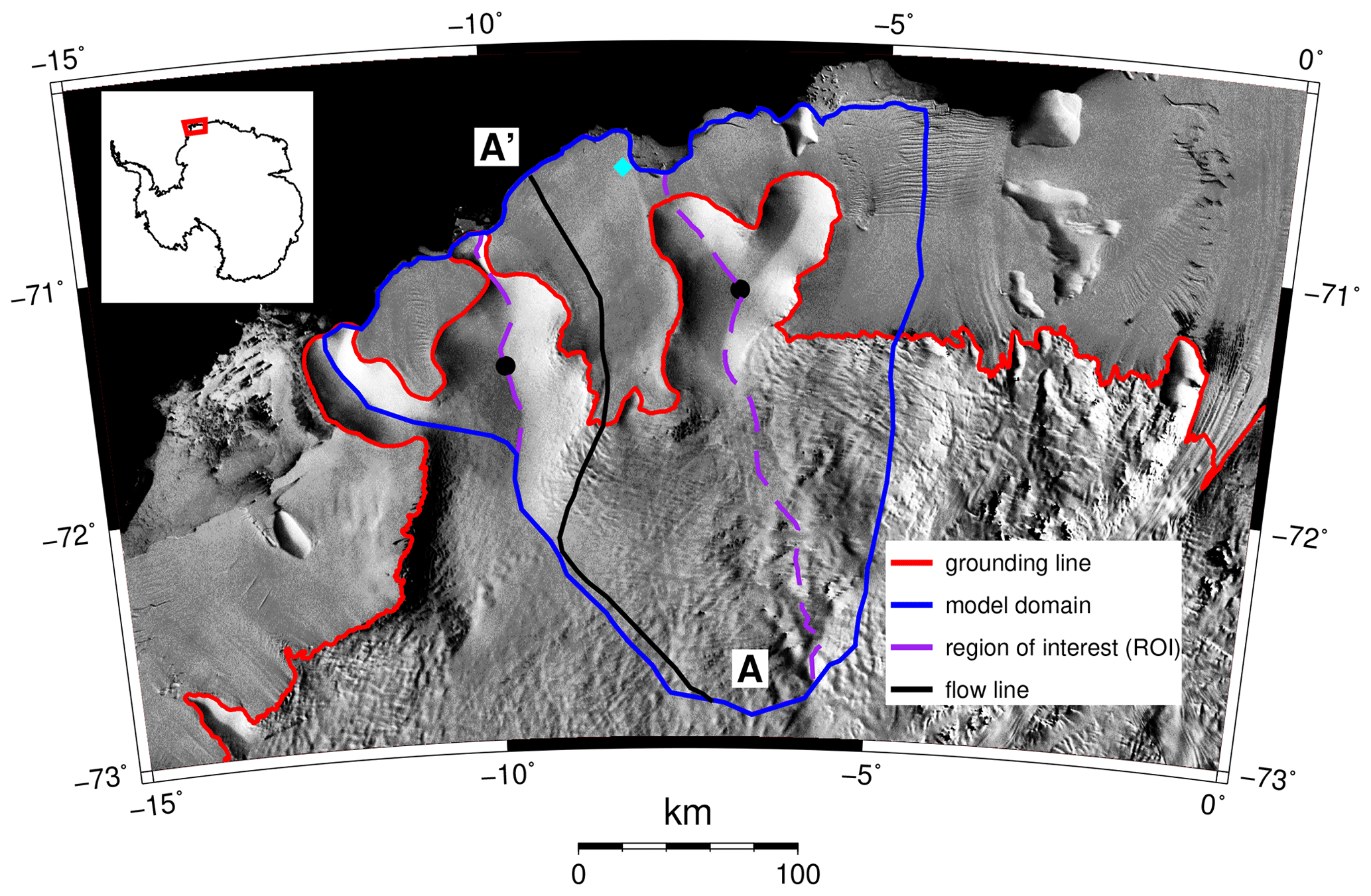
Figure 1 Overview of the Ekström Ice Shelf catchment with present-day grounding line (Bindschadler et al., 2011) and model domain. Cyan square shows location of Neumayer Station III. Filled black circles indicate location of ice rises. Flow line (A–A^′) is shown in Fig. 10. Background is the MODIS Mosaic of Antarctica (Scambos et al., 2007).

3 Model description

3.1 Ice flow equations

Ice flow is dominated by viscous forces which permits the dropping of the inertia and acceleration terms in the linear momentum equations. The Elmer/Ice ice sheet model (Gagliardini et al., 2013) solves the complete 3D equation for ice deformation. This results in the Stokes equations described by

$$\begin{array}{}\text{(1)}& \mathrm{\nabla }\cdot \mathit{\sigma }=-{\mathit{\rho }}_{\text{i}}\mathit{g}.\end{array}$$

Here, $\mathit{\sigma }=\mathit{\tau }-p\mathbf{I}$ is the Cauchy stress tensor, τ is the deviatoric stress tensor, $p=-tr\left(\mathit{\sigma }\right)/\mathrm{3}$ is the isotropic pressure, I is the identity tensor, ρ_i is the ice density, and g is the gravitational vector. Ice flow is assumed to be incompressible which simplifies mass conservation to

$$\begin{array}{}\text{(2)}& \mathrm{\nabla }\cdot \mathit{u}=\mathrm{0},\end{array}$$

with u being the ice velocity vector. Here we model ice as an isotropic material. Its rheology is given by Glen’s flow law which relates the deviatoric stress tensor τ with the strain rate tensor $\dot{\mathit{ϵ}}$:

$$\begin{array}{}\text{(3)}& \mathit{\tau }=\mathrm{2}\mathit{\eta }\dot{\mathit{ϵ}},\end{array}$$

where the effective viscosity η can be expressed as

$$\begin{array}{}\text{(4)}& \mathit{\eta }={\displaystyle \frac{\mathrm{1}}{\mathrm{2}}}B{\dot{{\mathit{ϵ}}_e}}^{\frac{(\mathrm{1}-n)}{n}}.\end{array}$$

In this equation, B is a viscosity parameter that depends on ice temperature relative to the pressure melting point computed through the Arrhenius law, n is Glen’s flow law parameter (n=3), and the effective strain rate is defined as ${\dot{{\mathit{ϵ}}_e}}^{\mathrm{2}}=tr\left({\dot{\mathit{ϵ}}}^{\mathrm{2}}\right)/\mathrm{2}$.

3.2 Ice temperature

The ice temperature is determined through the heat transfer equation (e.g. Gagliardini et al., 2013) which reads

$$\begin{array}{}\text{(5)}& {\mathit{\rho }}_{\text{i}}{c}_v\left({\displaystyle \frac{\partial T}{\partial t}}+\mathit{u}\cdot \mathrm{\nabla }T\right)=\mathrm{\nabla }\cdot \left(\mathit{\kappa }\mathrm{\nabla }T\right)+\dot{\mathit{ϵ}}\mathbf{:}\mathit{\sigma },\end{array}$$

where c_v and κ are the specific heat of ice and the heat conductivity, respectively. The : operator represents the colon product between two tensors. This last term of the equation represents strain heating. The ice temperature T is bounded by the pressure melting point T_m so that T≤T_m.

3.3 Boundary conditions

3.3.1 Ice temperature

Our parameterisation of surface temperature changes follows Ritz et al. (2001). We parameterise relative surface temperature changes to the present day as a function of relative surface elevation change with respect to present-day elevations and a spatially uniform surface temperature variation that is derived from the nearby EDML ice core (Graf et al., 2002). The surface temperature is then given by (Ritz et al., 2001, Eq. 11)

$$\begin{array}{}\text{(6)}& T_{\text{a}}=T_{\text{a0}}-{\mathit{\gamma }}_{\text{a}}(z_{\text{s0}}-z_{\text{s}})+\mathrm{\Delta }{T}_{\text{clim}}.\end{array}$$

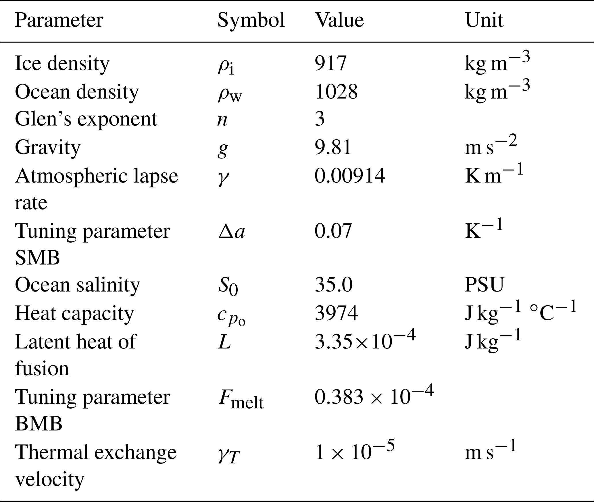
Here, T_a and T_a0 are the surface temperatures at the current time step and present day. The present-day temperature distribution is taken from Comiso (2000). z_s and z_s0 are the surface elevations at the current time step and present day, and ΔT_clim is the climatic forcing derived from the EDML ice core. As in Ritz et al. (2001), we apply a spatially constant lapse rate (γ_a) of 0.00914 K m⁻¹ (Table 1).

At the grounded base of the ice sheet, where the ice is in contact with the subglacial topography, we prescribe the geothermal heat flux (Martos et al., 2017). This heat flux is time invariant. Ice temperature is set to the local pressure melting point for the boundary condition underneath the floating ice shelves.

3.3.2 Surface mass balance (SMB) and basal mass balance (BMB)

A kinematic boundary condition determines the evolution of the upper and lower surfaces z_j:

$$\begin{array}{}\text{(7)}& {\displaystyle \frac{\partial z_j}{\partial t}}+u_x{\displaystyle \frac{\partial z_j}{\partial x}}+u_y{\displaystyle \frac{\partial z_j}{\partial y}}=u_z+{\dot{a}}_j,\end{array}$$

where ${\dot{a}}_j$ is the accumulation–ablation term and $j=(b,s)$, with s being the upper surface and b being the lower surface (base) of the ice sheet.

For the surface mass balance (SMB) parameterisation, we closely follow Ritz et al. (2001) again. We assume that no melt occurs in all our simulations. This is justified because SMB models simulate little melt in present-day conditions (Lenaerts et al., 2014) and these are the warmest years in our simulations. As for the surface temperature, our SMB parameterisation uses a present-day distribution of the SMB (Lenaerts et al., 2014) as input. Variations in the SMB over time are then proportional to the exponential of the surface temperature variation (Ritz et al., 2001, Eq. 12):

$$\begin{array}{}\text{(8)}& {\dot{a}}_{\text{s}}\left(T_{\text{a}}\right)=a_{\text{s0}}\left(T_{\text{a0}}\right)\exp \left(\mathrm{\Delta }a\right(T_{\text{a}}-T_{\text{a0}}\left)\right),\end{array}$$

where a_s0 is the present-day SMB, a_s is the SMB at the current time step, and the parameter Δa=0.07 K⁻¹. This means that for a surface temperature drop of 10 K, the SMB is reduced by 50 % (Ritz et al., 2001).

Sub-shelf melting underneath the floating ice shelves is based on the difference between the local freezing point of water under the ice shelves and the ocean temperature near the continental shelf break (Beckmann and Goosse, 2003). The freezing temperature (T_f) is calculated through

$$\begin{array}{}\text{(9)}& T_{\text{f}}=\mathrm{0.0939}-\mathrm{0.057}{S}_{\text{o}}+\mathrm{7.64}\times {\mathrm{10}}^{-\mathrm{4}}{z}_{\text{b}},\end{array}$$

where z_b is the base of the ice shelf and S_o is the ocean salinity (Table 1). The basal melt rates (${\dot{a}}_{\text{b}}$) are then computed by

$$\begin{array}{}\text{(10)}& {\dot{a}}_{\text{b}}={\displaystyle \frac{{\mathit{\rho }}_{\text{w}}{c}_{p_{\text{o}}}{\mathit{\gamma }}_{\text{T}}{F}_{\text{melt}}(T_{\text{O}}-T_{\text{f}}{)}^{\mathrm{2}}}{L{\mathit{\rho }}_{\text{i}}}}.\end{array}$$

In this equation, ρ_w is the density of water, $c_{p_{\text{o}}}$ is the specific capacity of the ocean mixed layer, γ_T is the thermal exchange velocity, L is the latent heat capacity of ice, F_melt is a tuning parameter to match present-day melt rates, and T_O is the ocean temperature (Table 1). The ocean temperature is initially set to −0.52 ^∘C (Beckmann and Goosse, 2003). F_melt is chosen such that present-day basal melt rates do not exceed ∼ 1.1 m yr⁻¹. This is in accordance with melt rates derived from satellite observations and mass conservation (Neckel et al., 2012). Applied variations in the ocean temperature are a damped (∼ 40 %) and delayed (∼ 3000 years) version of the climatic forcing for surface temperature ΔT_clim (Bintanja et al., 2005).

3.3.3 Basal sliding and sea level

Where the ice is in contact with the subglacial topography a linear Weertman-type sliding law of the form

$$\begin{array}{}\text{(11)}& {\mathit{\tau }}_{\text{b}}=C|{\mathit{u}}_{\text{b}}{|}^{m-\mathrm{1}}{\mathit{u}}_{\text{b}}\end{array}$$

is employed. Here τ_b is the basal traction, m is the basal-friction exponent which is set to 1 in all simulations, and C is the basal-friction coefficient. A linear viscous sliding relation (m=1) was chosen. Alternative and physically more realistic sliding relations exist (e.g. Joughin et al., 2019), and the consequences of our choice of using a linear sliding relation on the results are discussed below (see Sect. 5.5). For the present-day grounded ice sheet, C is inferred by solving an inverse problem (see Sect. 3.4), and for the present-day ocean beds a uniform basal-friction coefficient of 10⁻⁵ and 10⁻¹ MPa m⁻¹ yr is prescribed for the simulations of the soft (sediment-based) bed and hard (crystalline-rock-based) bed. Underneath the floating part of the domain, basal traction is zero (τ_b=0), but hydrostatic sea pressure is prescribed. We initialise the present-day sea level to zero and apply sea level variations according to Lambeck et al. (2014).

Table 1 Numerical values of the parameters adopted for the simulations.

3.4 Model initialisation

The model is initialised to the present-day geometry using the commonly applied snapshot initialisation in which the basal-traction coefficient C is inferred under the grounded ice sheet by matching observed surface velocities with modelled surface velocities. We take advantage of the quasi-steady state of the catchment and use the same optimisation parameters as in Schannwell et al. (2019). Similar to Zhao et al. (2018), we employ a two-step initialisation scheme. In the first iteration, the optimisation problem is solved with an isothermal ice sheet with ice temperature set to −10 ^∘C. The resulting velocity field is then used to solve the steady-state temperature equation before the optimisation problem is solved again with the new temperature field. This type of temperature initialisation approach provides similar results to a computationally more expensive temperature spin-up over several glacial cycles (Rückamp et al., 2018), as long as the system is close to a steady state.

3.5 Mesh generation and refinement

We initially create a 2D isotropic mesh with a nominal mesh resolution of ∼ 6 km everywhere in the domain. To ensure that we simulate grounding-line dynamics at the level of required detail, we use the meshing software Mmg (http://www.mmgtools.org/, last access: 28 February 2020) to locally refine the mesh down to ∼ 1 km in the region of the present-day Ekstöm Ice Shelf (Fig. 2) with areas away from the region of interest remaining at ∼ 6 km resolution. The mesh is then vertically extruded using 10 layers, and the horizontal mesh size is kept constant throughout the simulations. The 3D mesh consists of ∼ 200 000 nodes and therefore ∼ 800 000 degrees of freedom. We are using stabilised P1P1 elements and an algorithm that deduces a mass-conserving nodal surface to avoid artificial mass loss (Gagliardini et al., 2013).

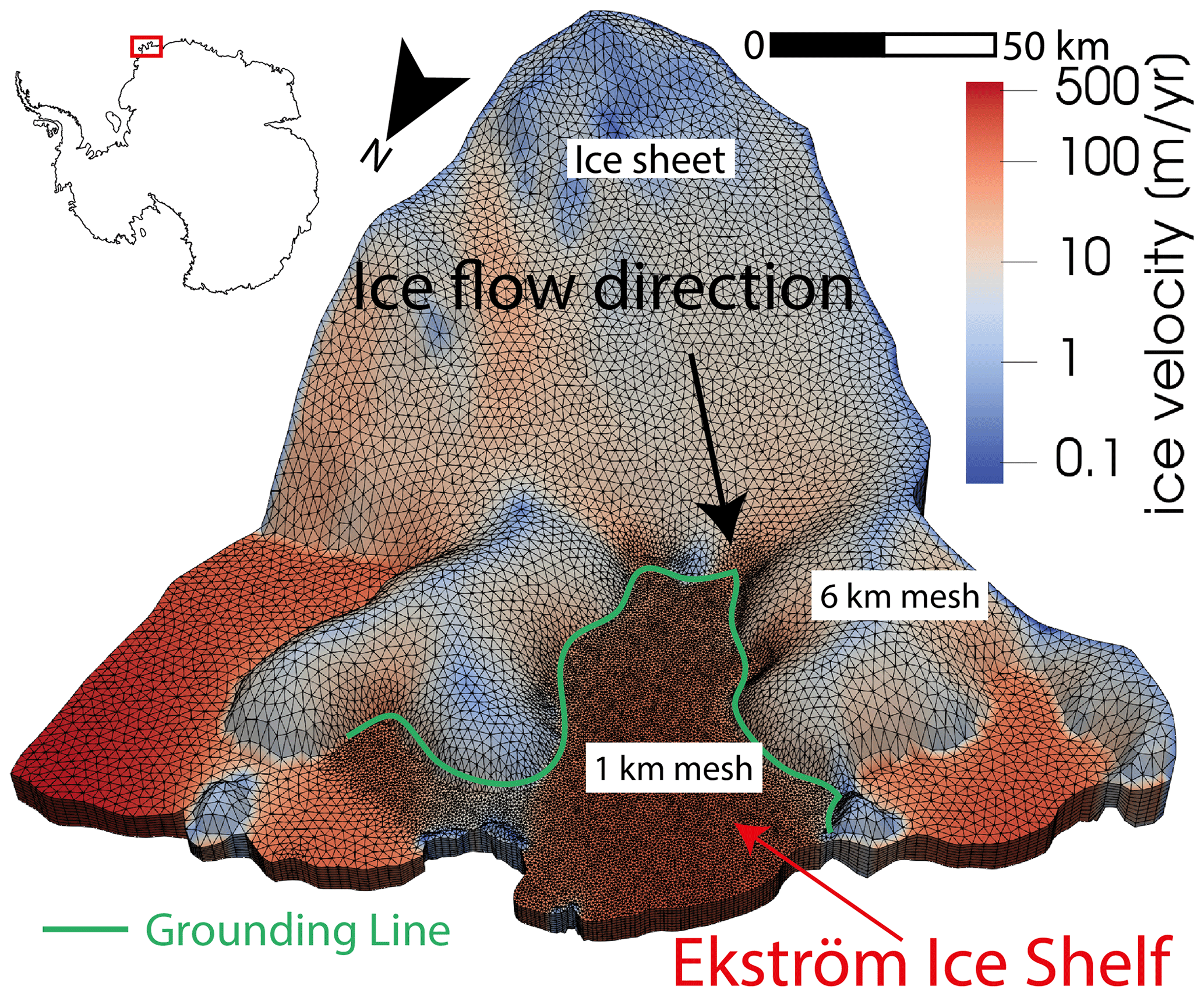
Figure 2 Model domain of Elmer/Ice in 3D including numerical mesh of Ekström Ice Shelf catchment, East Antarctica, with ice velocity in the background.

3.6 Block-preconditioned ParStokes solver

Because of the non-Newtonian rheology of ice and the dependence of viscosity on strain rates, the resulting Stokes equations are non-linear and have to be solved iteratively. In three dimensions the arising systems of linear equations become large (10⁶–10⁷ degrees of freedom) at a high mesh resolution. Standard iterative methods (Krylov subspace methods) in conjunction with algebraic preconditioners (e.g. incomplete lower–upper, ILU, decomposition) often do not converge for real-world geometries in glaciology. High aspect ratios of the finite elements and spatial viscosity variations of several orders of magnitudes strongly affect the accuracy and stability of the numerical solution (Malinen et al., 2013). This means that most glaciology applications with Elmer/Ice revert to using a direct method for solving the Stokes equations. While robust, direct solvers require large amounts of memory. In three dimensions their memory requirements increase with the square of the number of unknowns. Therefore, we use a stable parallel iterative solver (ParStokes) in our simulations that is implemented in Elmer/Ice but has so far been rarely used. ParStokes is based on block preconditioning (Malinen et al., 2013) that improves the solvability of the underlying saddle point problem through clustering of eigenvalues. As we will show below, the Krylov subspace methods now converge better and lead to improved scaling with more computer processing units (CPUs).

Figure 3 Scaling behaviour of iterative solver (ParStokes) and direct solver (MUMPS) for Elmer/Ice on the SuperMUC-NG supercomputer. Red square denotes number of CPUs selected for this study.

3.7 Experimental design

We demonstrate an FS simulation of ice sheet growth and decay over 40 000 years. During the first 20 000 years the atmospheric and oceanic forcing simulates the transition from an interglacial to a glacial period (henceforth called the advance phase). We then symmetrically reverse the climate forcing to simulate deglaciation (henceforth called the retreat phase). The symmetrical reversal of the model forcing enables investigation of hysteresis effects. The interglacial starting conditions are chosen with present-day properties and characteristics so that the best possible basal-friction coefficient beneath the grounded ice sheet can be found using today’s ice sheet geometry and surface velocities (Schannwell et al., 2019). The glacial conditions are chosen to resemble the Last Glacial Maximum for which we have good constraints for atmospheric forcing from the nearby EDML ice core. We consider two end-member basal property scenarios by prescribing either soft-ocean-bed conditions (mimicking sediment deposits) or hard-ocean-bed conditions (mimicking crystalline rock) under all present-day ice shelves in the modelling domain. The tested scenarios of basal-traction coefficients encompass what other ice sheet models have inferred (e.g. Cornford et al., 2015) for the grounded portion underneath the present-day Antarctic ice sheet (basal-traction coefficient ranging from 10⁻⁵ MPa m⁻¹ yr for sediments to 10⁻¹ MPa m⁻¹ yr for crystalline bedrock). Those end-member values do not reflect a true range of sliding coefficients for a given sliding law but were derived as tuning parameters. Hence they also account for some uncertainties in model parameters, forcings, and the physics of the applied ice sheet model. That is why we consider those values to be end members and regard simulated differences in ice volume and grounding-line position as the maximum envelope of uncertainties resulting from different ocean bed properties. We perform the simulations (a) with the standard Elmer/Ice setup using the MUltifrontal Massively Parallel sparse direct Solver (MUMPS) for ice velocities and (b) using a stable iterative solver for ice velocities (see Sect. 3.6), resulting in a total of four simulations. We carried out the simulations on two different high-performance computing systems: the ZDV cluster and the SuperMUC-NG system.

4 Results

The results can be divided into methodological advances and new scientific insights. In the following, we first present the technical improvements of the presented Elmer/Ice model setup in comparison to the “classic” setup employed in previous studies (e.g. Schannwell et al., 2019). This is followed by the analysis of the performed model simulations in terms of ice flow behaviour and an analysis of the role of the subglacial strata characteristics for advance and retreat dynamics.

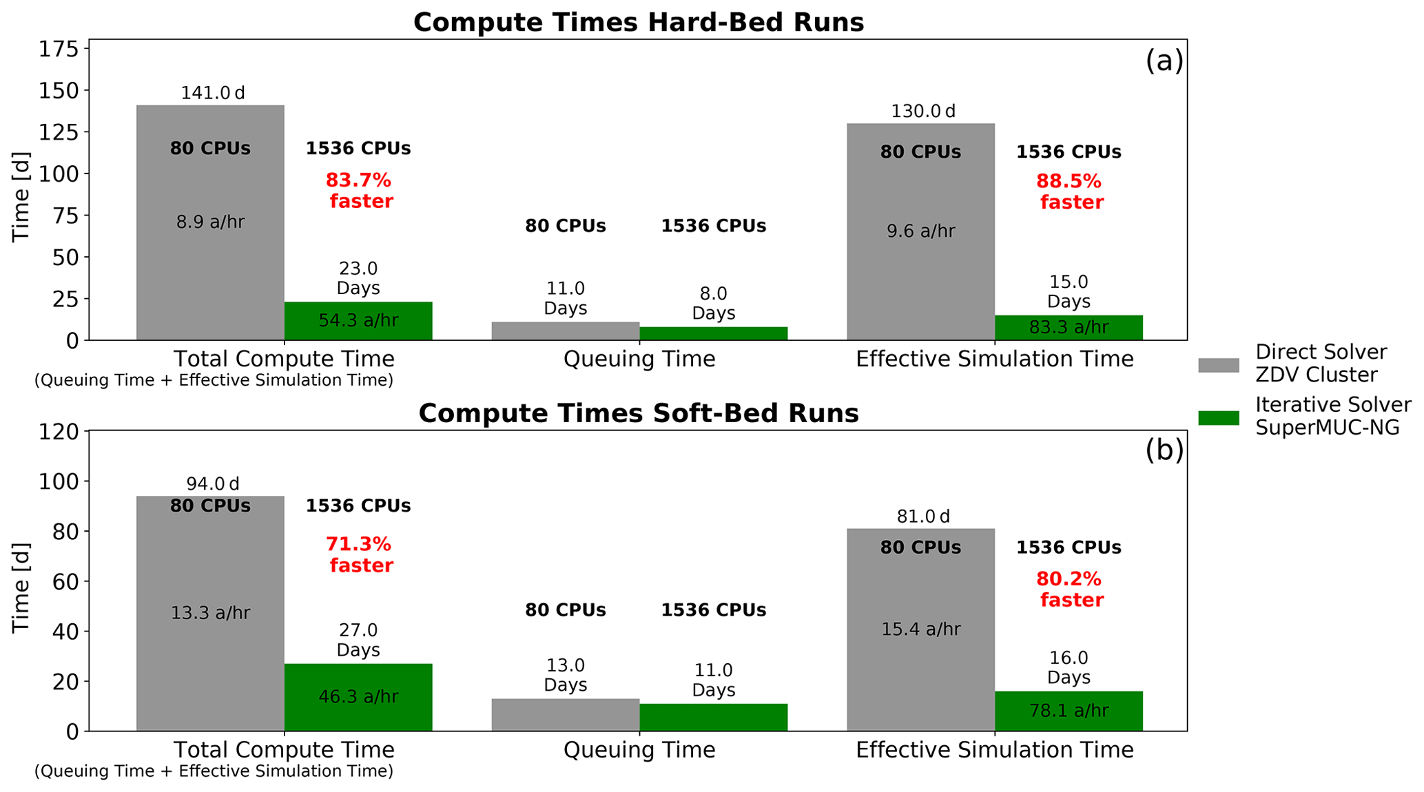
Figure 4 Speed-up of iterative solver (ParStokes, green bars) in comparison to direct solver (MUMPS, grey bars) for the hard-bed cavity (a) and soft-bed cavity (b) simulations. Simulations were performed on two different high-performance computing systems (ZDV and SuperMUC-NG).

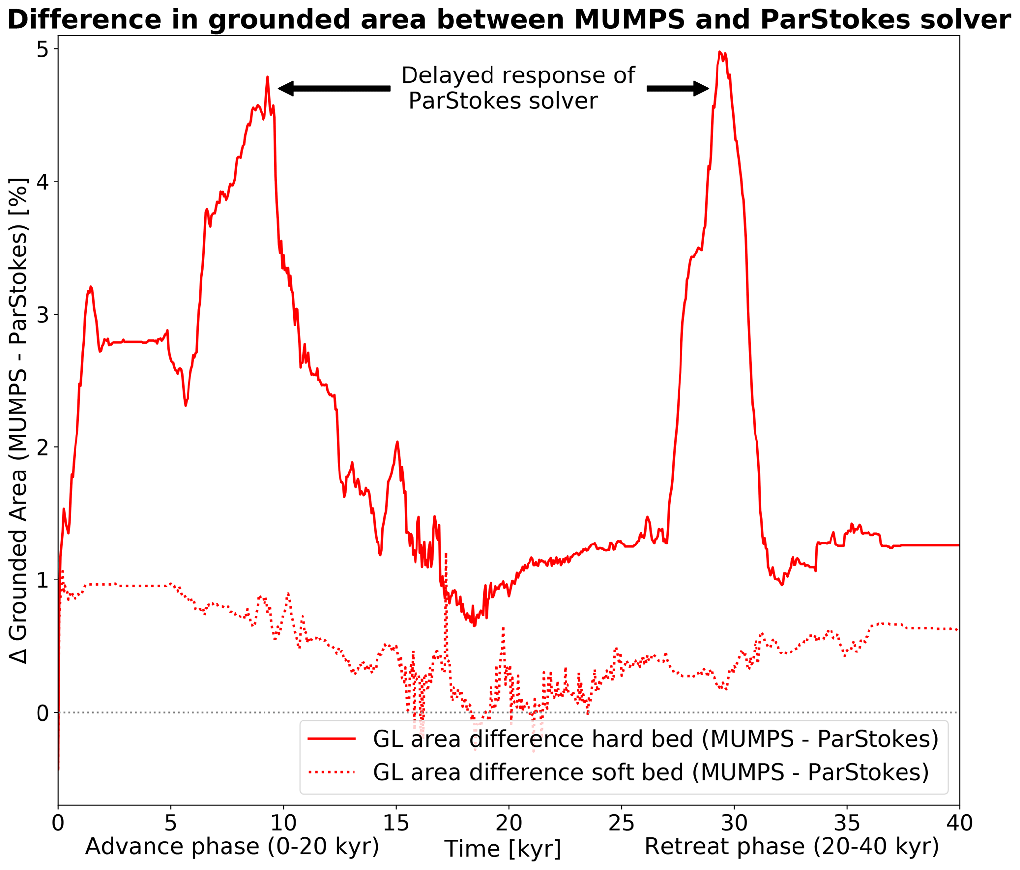
Figure 5 Differences in grounded area between the classic MUMPS and ParStokes solver setup for the soft-bed and hard-bed simulations.

4.1 Comparison between direct Stokes solver (MUMPS) and ParStokes

The ParStokes solver allows for a much better scaling of the required computation time with increasing numbers of CPUs (Fig. 3). While there is no speed-up for the “classic” solver setup using the direct solver MUMPS, there is a linear speed-up for the ParStokes solver up to ∼ 700 CPUs before the rate of speed-up tapers off and vanishes for more than 1536 CPUs. This much better scaling behaviour results in a total compute time for the iterative solver on the SuperMUC-NG system that is faster between a factor 3 and 6 in comparison to the MUMPS setup on the ZDV system. For our simulations, this means that the 40 000 year simulation now takes 23 d instead of 141 d for the hard-bed case, and 27 d instead of 94 d for the soft-bed case (Fig. 4). This speed-up is in part due to using more CPUs in the ParStokes simulations. When comparing the absolute runtime of the scaling simulations, ParStokes provides faster computations for > 168 CPUs. This means the minimum requirement for faster simulations with ParStokes is a supercomputer with more than 168 CPUs. The exact CPU number may however very well vary from system to system depending on the available hardware.

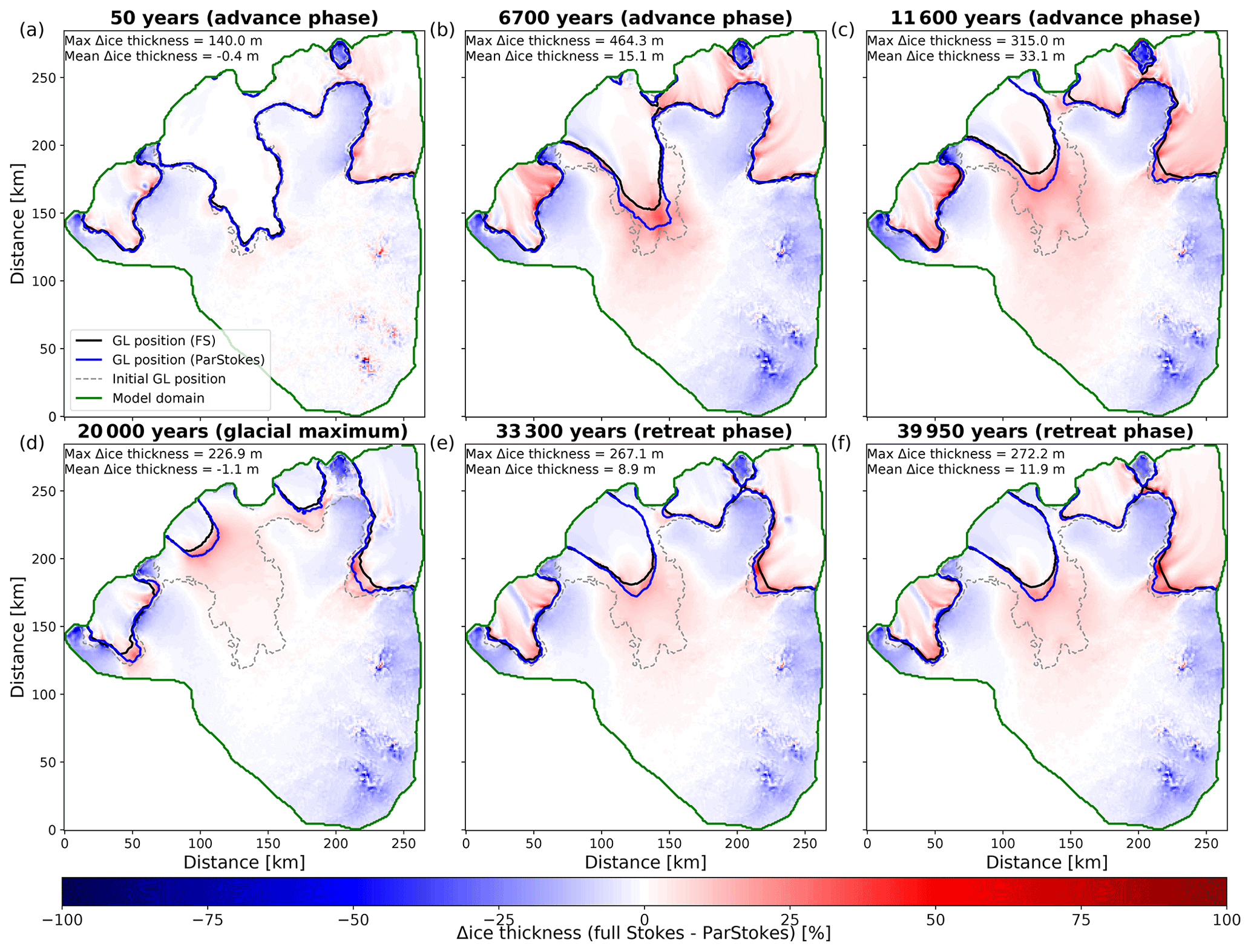
Figure 6 Differences in grounding-line position and ice thickness between the classic MUMPS and ParStokes solver setup for the hard-bed simulation at specific time slices.

We use predicted grounding-line position and ice thickness as metrics to compare the “classic” solver setup using MUMPS with the new solver ParStokes. We note however that we do not expect a perfect match between the two solver setups due to small differences in the finite-element formulation (e.g. stabilisation method). When using the solver MUMPS, the stabilised method is used, while for the ParStokes solver we use bubble stabilisation (Gagliardini et al., 2013). This results in slightly different systems that need to be solved. However, for both simulations, there is good agreement in terms of grounding-line position over time, with differences in grounded area never exceeding 5 % (Fig. 5). Because the soft-bed simulation exhibits smaller-magnitude grounding-line motion over the simulation, agreement between the two solver setups is better, with differences well below 1 % for almost the entire simulation length. In the hard-bed simulation, where larger magnitudes of grounding-line motion are predicted, the ParStokes solver's grounding line is not as far advanced as the solver MUMPS grounding line (Fig. 6). Moreover, at times of rapid grounding-line motion, the response of the grounding line in the ParStokes solver is delayed by up to ∼ 3500 years. This leads to differences in transient grounding-line positions (< 5 %). However grounding-line positions for the steady-state situation differ negligibly (<1.5 % difference). The predicted ice thickness differences are larger, particularly for the hard-bed run, where ice thickness change is larger overall. Locally these differences can be as large as ∼ 460 m (< 25 % of the ice thickness) in transient scenarios. They are most pronounced in periods of delayed grounding-line response. Once a stable grounding-line position has been reached, thickness differences are notably smaller (Figs. 6, 7). Overall, the ParStokes solver provides comparable results to the solver MUMPS but is much superior in terms of the required computation time. Therefore, the remainder of the results section will be based on the ParStokes solver simulations.

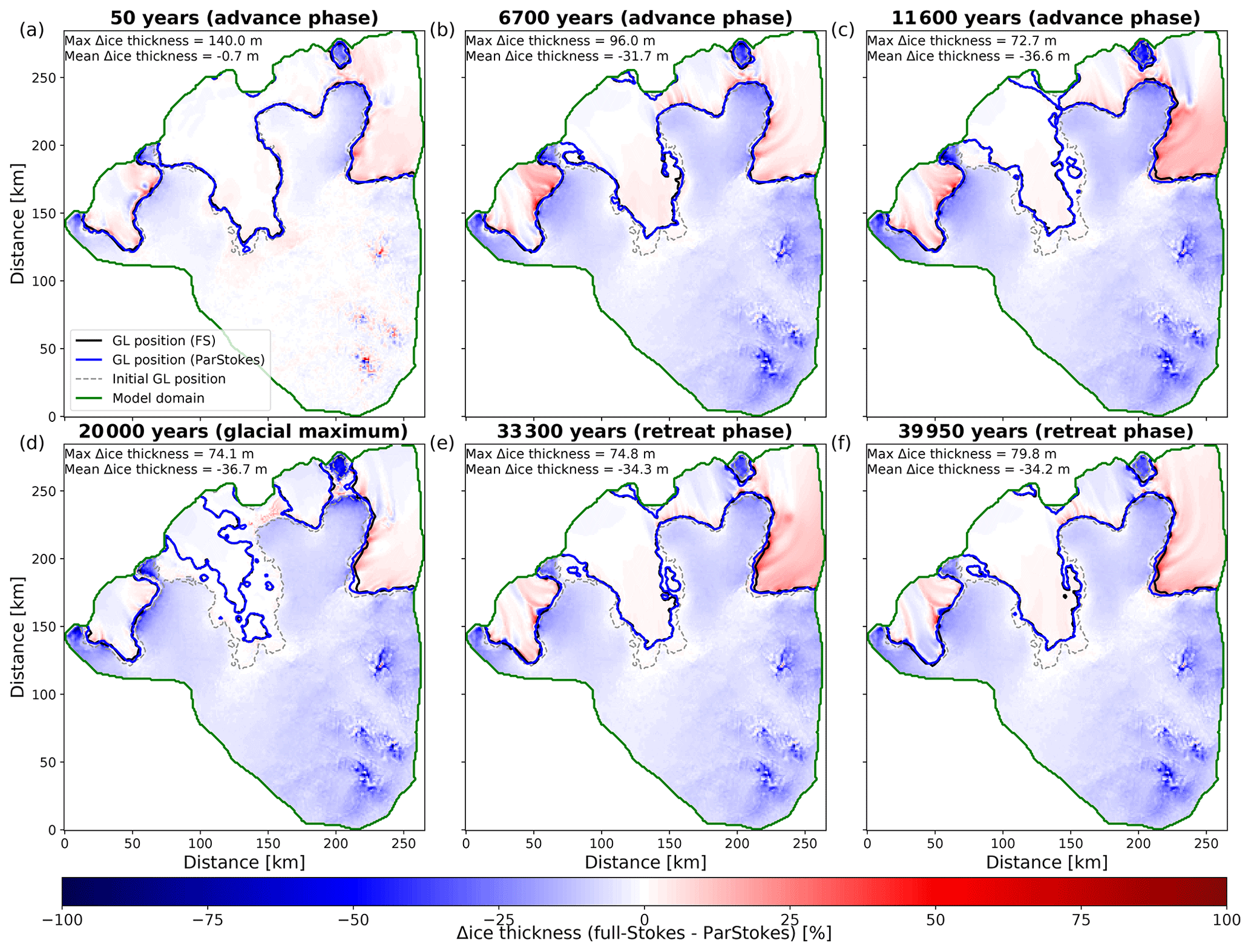
Figure 7 Differences in grounding-line position and ice thickness between the classic MUMPS and ParStokes solver setup for the soft-bed simulation at specific time slices.

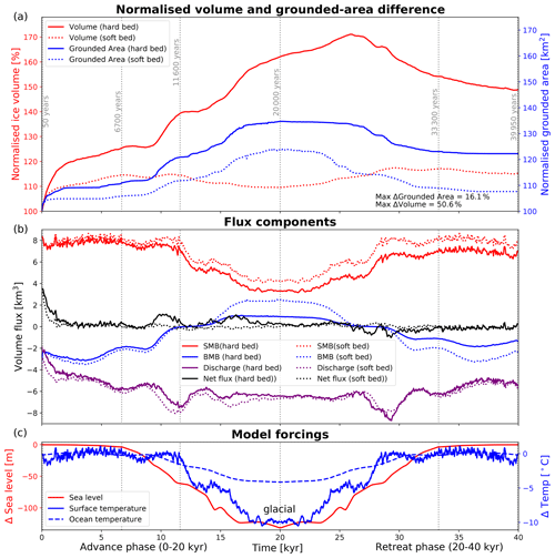
Figure 8 Ice sheet evolution and model forcing for soft- and hard-bed simulations. (a) shows volume and grounded-area evolution normalised to present day. (b) shows corresponding mass balance fluxes, and (c) shows most important model forcings. Vertical stippled grey lines show time slices shown in Figs. 6, 7, 9, and 10.

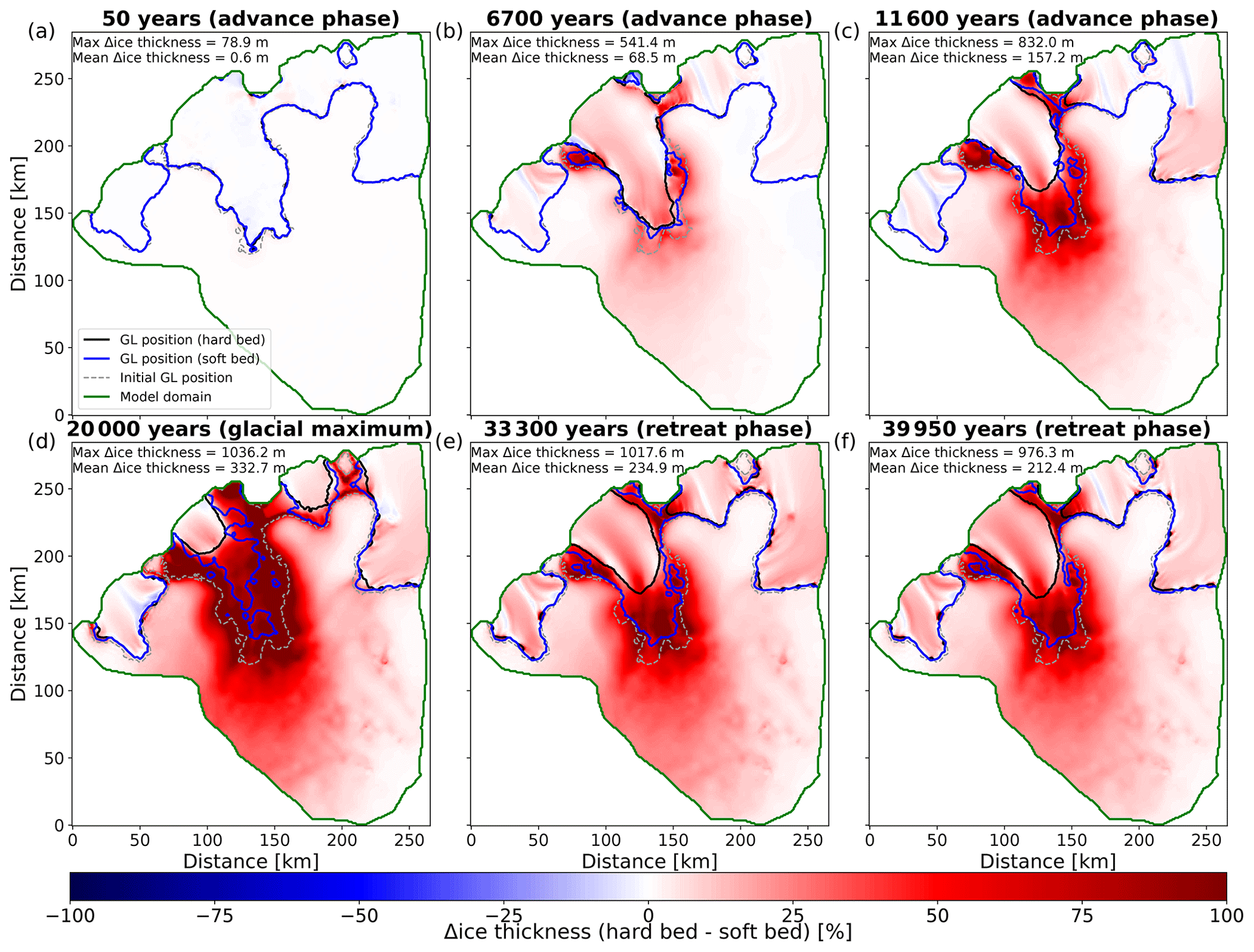
Figure 9 Differences in plane view of ice thickness and grounding-line positions between the hard- and soft-bed simulations at selected time slices. (a)–(d) show differences in the advance phase, and (e, f) show differences in the retreat phase.

4.2 Influence of bed hardness on ice sheet growth and decay

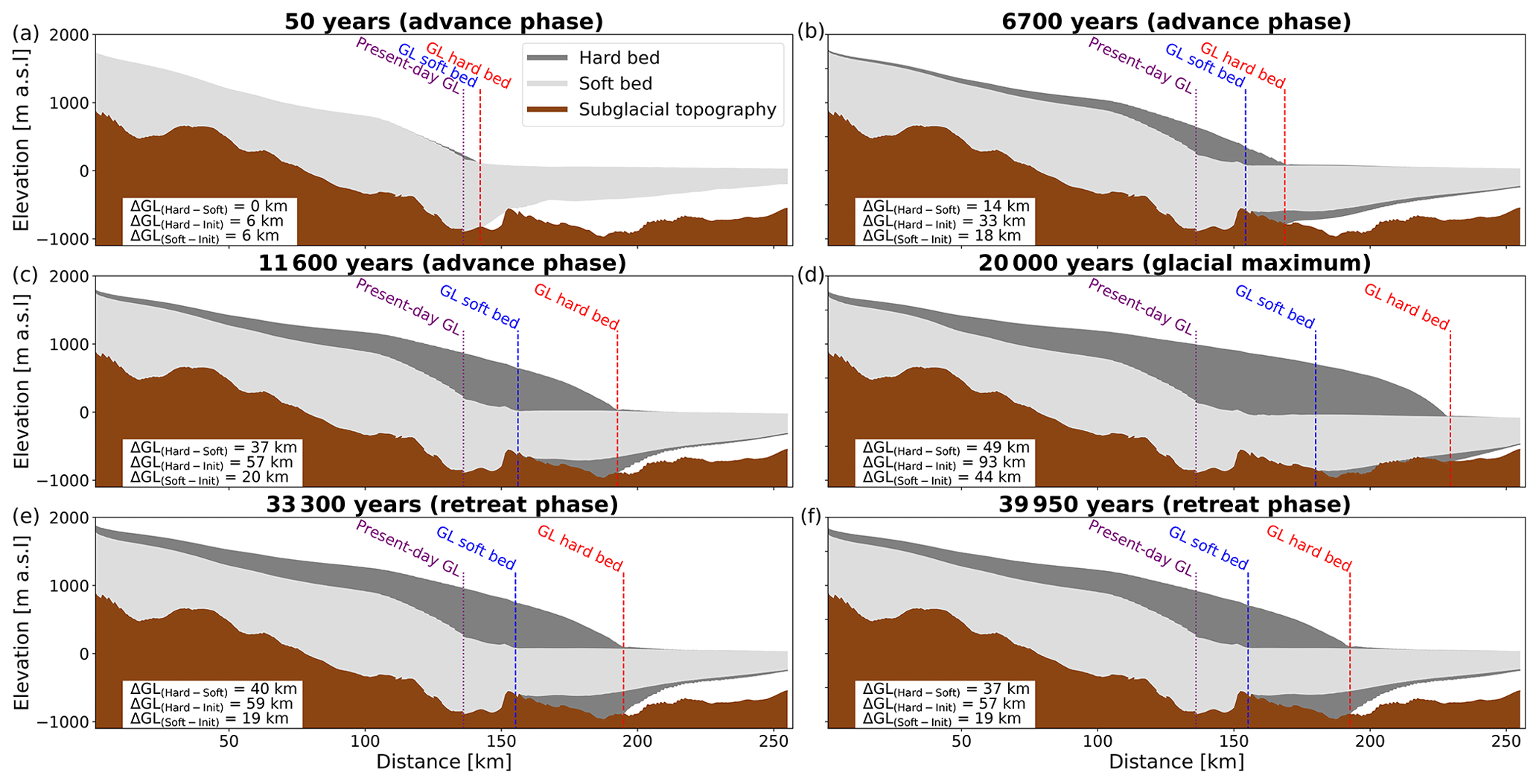
As expected, the hard- and soft-bed simulations result in different ice sheet geometries. Quantitatively, both scenarios differ significantly in transient- and steady-state volumes (Fig. 8), fluxes, and grounding-line positions (Figs. 9 and 10). The simulated hard-bed ice sheet is in many areas more than twice as thick as the soft-bed ice sheet, with maximum ice thickness differences between the hard and soft bed reaching 1036 m or 120 % (Fig. 10). In more detail, the differences between these simulations are as follows. First, the hard-bed ice sheet results in a thick, slow, and large-volume ice sheet after 20 000 years at glacial conditions. During the advance phase, volume increases occur step-wise with three distinct periods of volume increases (Fig. 8). These periods of volume increase in the region of interest are short (< 2000 years) and are interrupted by longer periods of little ice volume change. At the glacial maximum, the volume increase in comparison to the interglacial is ∼ 60 %. During the first ∼ 8000 years in the retreat phase, the hard-bed simulation continues to gain volume albeit at a slow rate. Following this period of volume gain, the ice sheet starts to lose volume. However, the rate of volume loss is small, such that after a full glacial cycle, the total ice volume is still ∼ 47 % more of what it was at the beginning of the simulation.

Second, unlike the hard-bed simulations, the soft-bed simulation leads to a thin, fast, and small-volume ice sheet at glacial conditions. During the advance phase, this simulation does not show a step-wise volume gain pattern. In fact, apart from an initial volume gain in the first 1000 years of the advance phase (∼ 10 %), there is very little volume change. This leads to a volume increase of merely ∼ 8 % at the glacial maximum. The trend of little volume variations continues during the retreat phase, where in the first 10 000 years a volume increase of ∼ 8 % occurs, before the volume remains approximately constant for the remainder of the retreat phase.

The entirely different ice sheet geometries for soft- and hard-bed simulations have consequences for the two ice rises present in the catchment (Fig. 1). While both ice rises and their divide positions are very little affected by the soft-bed simulations, they are partly overrun in the hard-bed simulation such that their local ice flow centre vanishes (see video supplement).

4.3 Grounding-line and ice sheet stability

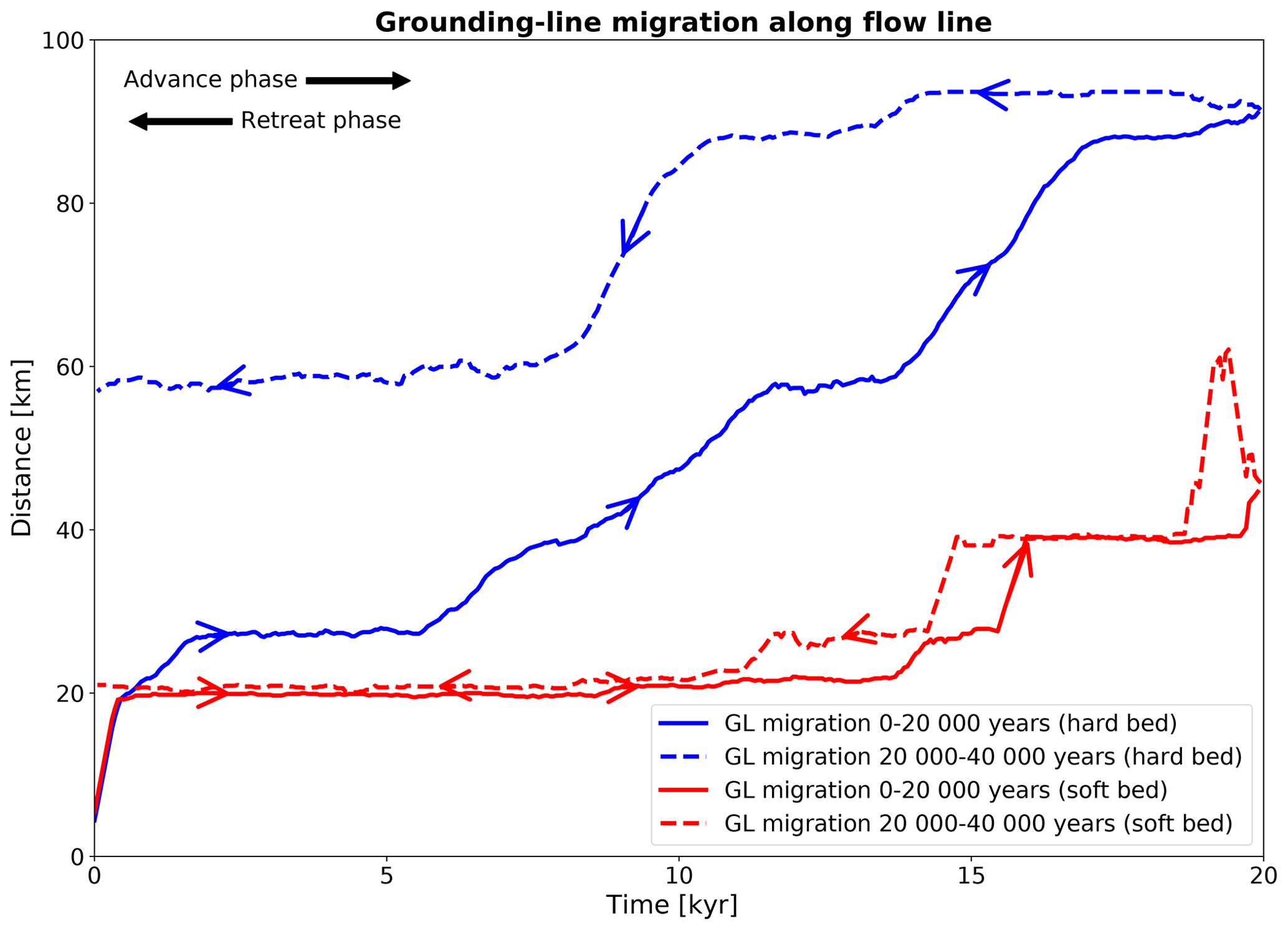
Steady grounding-line positions for both simulations are associated with periods of ice sheet stability (Fig. 8). There are three distinct periods of grounding-line stability in the advance phase and one period of grounding-line stability in the retreat phase. All four of these periods are longer than 3000 years. Periods of grounding-line advance in comparison are characterised by short leaps taking no longer than 1000–2000 years (Fig. 8). During the advance phase, differences in grounding-line positions between the hard-bed and soft-bed simulations gradually increase from 7 km after ∼ 1500 years to over 37 km after 11600 years and finally to a maximum difference of 49 km at the glacial maximum (Fig. 10). Grounding-line advance for the hard bed is more than twice as far (∼ 110 % larger) than its soft-bed counterpart in the advance phase. In the retreat phase, the soft-bed simulation shows higher grounding-line fidelity compared to the hard-bed simulation. The soft bed starts to exhibit grounding-line retreat after ∼ 4000 years into the retreat phase, whereas the hard bed does not show grounding-line retreat for ∼ 8000 years into the retreat phase.

4.4 Hysteresis of ice sheet simulations

Next we compare the ice sheet geometries during a full glacial cycle in which atmospheric and oceanic forcing are essentially symmetrically reversed. There is a significant grounding-line advance in the first ∼ 300 years in both simulations. In the following, hysteresis is analysed with respect to this position, rather than to the start of the simulation. Only the hard-bed simulation shows significant hysteresis behaviour, while the soft-bed simulation has negligible hysteresis (Fig. 11). For the hard-bed simulation, the grounding line after a full glacial cycle is ∼ 38 km further downstream of its initial position. This means that during the retreat phase, the grounding-line retreats only ∼ 48 % in comparison to the simulated grounding-line advance during the retreat phase of the hard-bed simulation.

5 Discussion

5.1 Extending the feasibility timescales of full-Stokes models

The inclusion of the iterative ParStokes solver results in a speed-up by a factor of 3–6 compared to the direct solver. While grounding-line positions agree well between the two solver setups, during periods of rapid grounding-line migration, positions can differ by up to ∼ 5 %. We note, however, that we do not expect a perfect match between the two solver setups due to small differences in the finite-element formulation (e.g. stabilisation method). Therefore, differences in grounding-line positions were expected between the solver setup, but they turn out to be small. The new setup now allows 3D full-Stokes ice sheet simulations on the regional scale over 40 000 years in under a month. We hereby maintain a mesh resolution (∼ 1 km) that is finer than in most other paleo ice sheet simulations (Pollard and DeConto, 2009; Golledge et al., 2014; Albrecht et al., 2020) albeit at a regional scale. However, while the time range is now significantly extended, our modelling approach only brackets the effect of ocean bed properties. As detailed below (Sect. 5.5), many other factors influencing ice sheet evolution, such as the applied BMB and SMB parameterisations and basal-sliding relation remain poorly constrained or are even excluded (e.g. glacial isostatic adjustment). Ensemble modelling (e.g. Golledge et al., 2012, 2014; Briggs et al., 2014; Pollard et al., 2016; Albrecht et al., 2020) using simplified ice physics is better suited for this, because these models can more easily include other important model sub-systems (e.g. basal hydrology, basal sliding) and evaluate their respective uncertainties.

Our efforts aim to include higher-order ice physics in paleo ice sheet simulations. The advantages of our FS simulations are as follows. By retaining all terms in the force balance, we have a solid physical representation of internal deformation and grounding-line dynamics over glacial timescales. This permits an improved quantification of the relative contributions from basal sliding and ice deformation to the column-averaged ice discharge, opening the door for a better understanding of basal processes such as erosion and deposition of sediments and the formation of ice streams. We are also able to quantify the effect of ocean bed properties on the grounded ice sheet as the backstress provided by the contrasting ocean bed properties is correctly transmitted upstream by our FS model. Grounding-line migration also needs to be interpreted in relation to observed bedforms. For example, the bedrock bump at 150 km in Fig. 10 is interpreted as a potential overdeepening, carved out by the confluence of two paleo ice streams (Smith et al., 2020). Our study presents the numerical framework to test hypotheses such as this. Even though we are still not able to constrain our model with paleo observations due to the computation requirements, our study provides an important first step towards it. In addition, computing the full 3D ice velocity field from the linear momentum equations may help to include thus far unused paleo data as constraints. For example, radar isochrones for floating ice shelves could be incorporated more easily into the model tuning, because the FS approach does not apply a vertical average in these areas unlike ice models using a simplified force balance. We believe that ensemble modelling using simpler ice physics models and our approach of employing a complex ice physics model and investigating end-member scenarios can both provide different new insights. Hence, both approaches should be pursued in future. This also holds for shallow-ice approximation–FS hybrid approaches (Ahlkrona et al., 2016) which can build on the results shown here.

Figure 10 Difference in ice sheet geometry and grounding-line position along a flow line (A–A^′ in Fig. 1) for the soft- and hard-bed simulations. (a)–(d) show differences in the advance phase, and (e, f) show differences in the retreat phase.

5.2 Influence of bed hardness on ice sheet growth and decay

The completely different ice sheet geometries for the hard- and soft-bed simulations are a consequence of the different levels of basal friction provided by the hard and soft bed, respectively. The predicted differences between the hard-bed and soft-bed simulations underline the high significance of a proper choice of basal properties used for ocean beds. The higher basal friction in the hard-bed case leads to elevated backstress and corresponding dynamical thickening of the inland ice sheet far upstream of the grounding line. Although the SMB and BMB forcings equally depend on the ice sheet geometry through the applied parameterisations, these effects are small compared to the dynamically induced ice thickening (Fig. 9). This clearly shows that in the absence of other forcing mechanisms, ocean bed properties exert an important control on ice sheet growth and decay.

The importance of ocean bed properties on ice sheet evolution has long been known (e.g. Pollard and DeConto, 2009; Whitehouse et al., 2012; Pollard et al., 2016; Whitehouse et al., 2017; Albrecht et al., 2020). Here we quantify upper and lower bounds of this effect for the first time on a regional scale with an FS model. Our results indicate that spatial changes in basal-friction coefficients in the cavities are likely very important for ice sheet growth and decay behaviour. This is relevant for the Ekström Ice Shelf embayment and probably most of Dronning Maud Land, as evidence from geophysical data shows that the ocean bed of the Ekström cavity consists at least partly of crystalline bedrock (Kristoffersen et al., 2014; Smith et al., 2020). This feature is more than 1000 km long. A new compilation and interpretation of airborne geophysics data by Eisermann et al. (2020) shows that the northern edge of a strong magnetic anomaly coincides with the location of the outcrop of the volcanic Explora Wedge (Smith et al., 2020), where subglacial material changes from ocean sediments to crystalline rock. This transition cross-cuts the Ekström Ice Shelf cavity from ENE to WSW over its full width. Based on our simulations, such crystalline outcrops under ice shelves will result in a thicker but slower ice sheet over the last glacial cycle, compared to a thin and fast ice sheet linked to soft ocean beds which are mostly assumed for areas that lie below the present-day sea level (Pollard and DeConto, 2009; Pollard et al., 2016; Whitehouse et al., 2017). Interestingly, today's north-easternmost grounding line of Halfvarryggen ice rise coincides with this magnetic anomaly and the Explora Volcanic Wedge outcrop and thus likely with the presence of subglacial crystalline strata (Smith et al., 2020; Eisermann et al., 2020). We can therefore hypothesise that the spatial variations in subglacial strata also influence the position of present-day grounding lines. Finally, the ramifications of heterogeneous ocean bed properties go beyond ice volume considerations. Different levels of basal traction strongly affect the magnitude of basal sliding. This in turn determines how much material is eroded underneath the ice sheet and transported across the grounding line. As erosion rates are commonly approximated as basal sliding to some power (e.g. Herman et al., 2015; Alley et al., 2019; Delaney and Adhikari, 2019), any differences in basal-sliding velocities are exacerbated when erosion volumes are computed. This uncertainty in eroded material produced has implications for how much sediment is available at the ice–bedrock interface and therefore if it is a hard- or soft-bed interface and its temporal variability.

Figure 11 Grounding-line migration along a flow line (A–A^′ in Fig. 1) for the soft- and hard-bed simulations for the advanced (solid lines) and retreat (dashed lines) phase.

5.3 Grounding-line and ice sheet stability

The identified stable grounding-line positions are not controlled by a single specific forcing alone but are due to a combination of sea level forcing, basal traction of the ocean bed, and ocean bathymetry. Other forcing mechanisms such as the SMB and BMB are of secondary importance. However, the relative stability of grounding-line position (< 7 km of grounding-line retreat) in the last 9000 years of the retreat phase in both simulations coincides with the period of few sea level variations, leading us to conclude that at least for the retreat phase, sea level forcing is the most important model forcing. The earlier onset of grounding-line motion in the retreat phase for the soft bed can be attributed to the fact that ice discharge for the soft-bed simulation is dominated by basal sliding and higher ice velocities. In comparison, in the hard-bed simulation ice discharge is dominated by internal deformation and almost no basal sliding, resulting in a much thicker ice sheet. This means that more ice needs to be removed before the grounded ice can detach from its subglacial material and initiate grounding-line motion, thereby resulting in a much slower response time to changes in the model forcing. While our employed modelling approach makes it unlikely that the timings of our modelled stable grounding-line positions are correct, they can still serve as rough spatial markers of areas where depositional landforms such as grounding-zone wedges or other geomorphological markers may be found.

5.4 Hysteresis of ice sheet simulations

We attribute the modelled grounding-line advance in the first ∼ 300 years to the fact that our ice sheet geometry is not completely in a steady state after initialisation. This is due to inconsistencies of the model forcing (e.g. BMB parameterisation) in combination with boundary datasets (e.g. cavity topography). However, this does not affect our conclusions regarding ice sheet hysteresis. Our results highlight the importance of different ocean bed properties for the ice sheet's hysteresis behaviour. This underlines the dependence of the final ice sheet geometry on the model’s initial state over timescales of a glacial cycle or longer. While bedrock geometry has long been identified as a cause for hysteresis behaviour in ice sheet models (e.g. Schoof, 2007) and remains an important indicator for future ice sheet vulnerability, our simulations show that in the absence of retrograde-sloping bedrock topography, varying ocean bed properties also have the potential to induce hysteresis. However, this result could also be caused by a combination of the non-uniqueness of the Stokes contact problem for non-sliding beds and an under resolving of the grounding-line zone (e.g. Nowicki and Wingham, 2008). Despite very similar model forcing, our simulations result in a non-linear response of ice sheet evolution that is exclusively controlled by ocean bed properties, revealing an additional challenging problem for model simulations over at least one advance and retreat cycle (Pollard and DeConto, 2009; Gasson et al., 2016). This also means that the employed modelling framework will likely not result in the correct ice sheet geometry at the LGM due to non-linear feedback mechanisms such as the marine ice sheet instability (Schoof, 2007; Durand et al., 2009), the height–mass balance feedback (Oerlemans, 2002), and remaining uncertainties regarding the subglacial topography.

5.5 Model limitations

The primary focus of the modelling framework was to extend the applicability of FS ice sheet models to glacial-cycle timescales. This means that simplifications were made to other model components that we list here. We regard each of these simplification as a future avenue to improve upon the presented results.

The modelling approach presented here is tailored towards capturing ice and grounding-line dynamics to a high accuracy at the cost of comparatively naive parameterisations for the SMB and BMB which can be improved in the future. Also, by approximating hard and soft ocean beds through a time- and space-invariant friction coefficient, we omit spatial gradients in the thickness, grain size, and cohesion of the ocean bed substrate. We therefore assume that properties of hard-bed and soft-bed areas at the start of the simulation remain constant throughout the simulation. This means areas in which little or enhanced basal sliding occurs in the modelling domain stay constant.

At the underside of the grounded ice sheet, we use a linear Weertman sliding law that relates the basal shear stress to the basal-sliding velocity. In comparison to the non-linear Weertman sliding law, the linearised version has a tendency to reduce grounding-line fidelity (e.g. Schannwell et al., 2018; Brondex et al., 2019). While this type of sliding law is still widely used (e.g. Ritz et al., 2015; Cornford et al., 2015; Nias et al., 2016; Yu et al., 2017; Schannwell et al., 2018; Brondex et al., 2019), pressure-limited sliding relations (e.g. Tsai et al., 2015) are becoming more popular in the modelling community. The difference between Weertman and pressure-limited relations is that the latter take effective pressure into account. This means that basal drag goes to zero near the grounding line and reduces to a plastic-sliding relation (Brondex et al., 2017). This results in the basal drag becoming independent of the sliding velocity. Most previous studies using pressure-limited relations confine areas of lower basal drag to within a few kilometres upstream of the grounding line (e.g. Schannwell et al., 2018; Brondex et al., 2019). There is however evidence from observations and modelling that areas of low basal drag can extend much farther inland (Joughin et al., 2019). Studies that have investigated the effect of the different sliding laws on grounding-line retreat have found that the pressure-limited relations lead to enhanced grounding-line retreat (e.g. Schannwell et al., 2018; Brondex et al., 2019) in comparison to Weertman sliding laws. However, it is difficult to judge how much a pressure-limited sliding law would affect our results as up to now no study has investigated this effect over an advance and retreat cycle.

Moreover, we have not considered glacial isostatic adjustment (GIA). Until recently, GIA was considered to be only important on timescales exceeding 1000 years. However, recent progress has revealed that due to lower than previously assumed mantle viscosities, response times of GIA to ice unloading can be as short as 5 years for certain sections in Antarctica (Barletta et al., 2018; Whitehouse et al., 2019). While present-day GIA rates for East Antarctica are relatively low (∼ 1 mm yr⁻¹; see Martín-Español et al., 2016) in comparison to regions of high mass loss in Antarctica, the effect over 20 000 years could amount to ∼ 20 m of elevation drop for the subglacial topography. This number is small in comparison to, for example, sea level variations (∼ 130 m) but may nevertheless result in a grounding-line position that is not as far advanced at the glacial maximum as presented in our simulations.

6 Conclusions

Our simulations unlock a new time dimension for the applicability of FS ice sheet models on the regional scale. Application of an iterative solver reduced computation times in comparison to previous simulations by ∼ 80 % and extended the temporal range of FS simulations by a factor of 40 compared to previous studies. This provides an important step towards including higher-order physics in paleo ice sheet simulation and reduces uncertainties arising from approximations to the ice flow equations. Being able to simulate ice deformation to a high accuracy over glacial timescales also opens opportunities for a better understanding of a number of subglacial processes (e.g. basal erosion).

We find ice volume differences of > 50 % over a glacial cycle that are exclusively caused by differing ocean bed properties. The different ocean bed properties also result in different ice sheet growth and decay patterns with the thick and slow-flowing hard-bed simulation exhibiting strong hysteresis behaviour. This is completely absent in the thin and fast-flowing soft-bed simulation. As recent geophysical observations (e.g. Gohl et al., 2013; Smith et al., 2020; Eisermann et al., 2020) indicate a more heterogenous substrate distribution (sediments vs. crystalline bedrock) than previously thought, this could have important consequences for past stable ice sheet geometries and grounding-line positions as well as for the present and future response of the ice sheet's grounding line to ocean warming.