the Creative Commons Attribution 4.0 License.
the Creative Commons Attribution 4.0 License.
 | 09 Nov 2020
Recent changes in pan-Antarctic region surface snowmelt detected by AMSR-E and AMSR2
Lei Zheng
Chunxia Zhou
Tingjun Zhang
Qi Liang
Kang Wang
Surface snowmelt in the pan-Antarctic region, including the Antarctic ice sheet (AIS) and sea ice, is crucial to the mass and energy balance in polar regions and can serve as an indicator of climate change. In this study, we investigate the spatial and temporal variations in surface snowmelt over the entire pan-Antarctic region from 2002 to 2017 by using passive microwave remote sensing data. The stable orbits and appropriate acquisition times of the Advanced Microwave Scanning Radiometer for the Earth Observing System (AMSR-E) and the Advanced Microwave Scanning Radiometer 2 (AMSR2) enable us to take full advantage of daily brightness temperature (Tb) variations to detect surface snowmelt. The difference between AMSR-E/2 ascending and descending 36.5 GHz Tb values in vertical polarization (DAV36) was utilized to map the pan-Antarctic region snowmelt, as this method is unaffected by snow metamorphism. We evaluated the DAV36 algorithm against ground-based measurements and further improved the method over the marginal sea ice zone by excluding the effect of open water. Snowmelt detected by AMSR-E/2 data was more extensive and persistent than that detected by the Special Sensor Microwave/Imager (SSM/I) data. Continuous melt onset (CMO) ranged from August in the marginal sea ice zone to January in the Antarctic inland, and the early transient melt events occurred several days to more than 2 months earlier. The pan-Antarctic region CMO was significantly correlated (R=0.54, p<0.05) with the summer Southern Annular Mode (SAM). The decreased AIS melt extent was very likely linked (, p<0.01) with the enhanced summer SAM.
- Article
(13880 KB) - Full-text XML
-
Supplement
(4996 KB) - BibTeX
- EndNote


Surface snowmelt on sea ice and ice sheets has a great influence on the energy exchange between the snow surface and atmosphere because wet snow has a lower albedo and thus absorbs more incoming solar radiation than dry snow (Steffen, 1995). Intense snowmelt leads to the formation of melt ponds on sea ice and ice sheets, which in turn absorb more radiation and induce further snowmelt through melt–albedo feedback (Tanaka et al., 2016; Bell et al., 2018). Meltwater may fill in the ice crevasses on ice sheets and migrate to the ice–bedrock surface, which can induce the acceleration of ice flow (Zwally et al., 2002; Sundal et al., 2011). Meltwater can also transport heat into crevasses and deepen them, providing the conditions for ice shelves to break up through hydrofracturing (Scambos et al., 2000; van den Broeke, 2005). Therefore, the spatial and temporal dynamics of surface snowmelt on sea ice and ice sheets have a direct effect on mass and energy balances in polar regions (Picard and Fily, 2006; van den Broeke et al., 2009; Stroeve et al., 2014). The timing and extent of surface snowmelt are indicators of changes in polar climate (Intergovernmental Panel on Climate Change (IPCC), 2014) and thus potentially have regional and global climate implications.
Unlike the Arctic sea ice and Greenland ice sheet, pan-Antarctic surface snowmelt is relatively short-lived and patchy (Drinkwater and Liu, 2000; Picard et al., 2007) and has received much less attention. Unlike the reductions in sea ice extent, thickness and duration in the Arctic, the Antarctic sea ice has presented increasing trends in both extent and duration, especially in the Ross Sea (Comiso and Nishio, 2008; Hobbs et al., 2016). Most of the Antarctic sea ice is snow-covered, even in summer when snowmelt occurs (Brandt et al., 2005). Melt ponds are not often observed on the Antarctic sea ice (Ackley et al., 2008). Meltwater on the Antarctic ice sheet (AIS) can refreeze quasi-instantaneously (van den Broeke et al., 2010a) and contributes little to the surface mass balance (The IMBIE team, 2018). Although more than 25 % of the AIS has experienced snowmelt since the 1980s, only 2 % melts every year (Picard et al., 2007). The melt extent has been decreasing over the AIS since 1987 (Tedesco et al., 2007).
In situ observations of snowmelt are sparse over sea ice and ice sheets due to an unfavorable environment. Remote sensing techniques can provide timely data sets for the monitoring of melt events in polar regions. When a snowpack begins to melt, the most significant change in its electromagnetic properties is an abrupt increase in the dielectric constant, which increases absorption and reduces the penetration depth of microwaves (Ashcraft and Long, 2006). Therefore, snowmelt can be detected via microwave radiometry by identifying the sharp changes in microwave measurements caused by the presence of snow liquid water (Serreze et al., 1993; Liu et al., 2005).
Microwave radiometers can operate regardless of illumination conditions and are insensitive to atmospheric conditions. Most spaceborne passive microwave instruments provide more than two daily passes in polar regions. Scanning Multichannel Microwave Radiometer (SMMR) 18 and 37 GHz brightness temperatures (Tb) and Special Sensor Microwave/Imager (SSM/I) 19 and 37 GHz Tb have been used to detect surface snowmelt on ice sheets when Tb values are above a region-specific or user-defined constant depending on the local snow properties (Ridley, 1993; Zwally and Fiegles, 1994; Mote and Anderson, 1995; Tedesco, 2009). Tb values received by satellites are also related to the ground physical temperature, clouds and atmospheric water vapor, which may contaminate melt signals in a Tb time series. Multichannel methods have been developed to minimize these interferences, e.g., using a gradient ratio or a cross-polarized gradient ratio (XGPR) between 19 and 37 GHz to detect surface snowmelt on sea ice and ice sheets (Abdalati and Steffen, 1995; Markus et al., 2009; Liang et al., 2013; Arndt et al., 2016). Snowmelt can also be recognized based on edge detection or wavelet-transform-based technologies by identifying the abrupt changes in Tb values (Joshi et al., 2001; Liu et al., 2005).
The beginning of a melt season is characterized by a sharp increase in Tb due to the freeze–thaw cycle. The snow grain size increases after the liquid water refreezes. As a result, Tb may decrease during the melt season due to the increase in volume scattering (Markus et al., 2009). Therefore, single-channel methods may fail to identify melt events because of the metamorphic snow structures. Ramage and Isacks (2002, 2003) introduced SSM/I diurnal amplitude variations (DAVs, i.e., the Tb difference between ascending and descending passes) in vertically polarized 37 GHz Tb to investigate the snowmelt timing on the southeast Alaskan ice fields and showed that the DAV method can stably recognize melt events. The DAV technique has been successfully applied to ice sheets and has been proven more sensitive to snow liquid water than the XGPR method (Tedesco, 2007; Zheng et al., 2018). Freeze–thaw cycles on the Antarctic sea ice were also successfully detected based on the SSM/I 37 GHz DAV (Willmes et al., 2009). Furthermore, Arndt et al. (2016) distinguished temporary snowmelt from continuous snowmelt on the Antarctic sea ice by combining DAV with a cross-polarized ratio of SSM/I Tb. In these studies, surface snowmelt patterns were not described over the marginal sea ice zone, where the earliest sea ice retreat was identified (Stammerjohn et al., 2008) and where DAV may not be strong enough to be identified as melt signals when open water with a low Tb emerges in the first-year sea ice zone.
Most of these studies investigated surface snowmelt on sea ice and ice sheets based on SSM/I sensors. However, SSM/I observations show considerable variations in local acquisition time because of orbit degradation (Picard and Fily, 2006). In contrast, the Advanced Microwave Scanning Radiometer for the Earth Observing System (AMSR-E) and the Advanced Microwave Scanning Radiometer 2 (AMSR2) operate in controlled orbits so that local acquisition time shows little temporal variation (http://www.remss.com/support/crossing-times, last access: 12 August 2020). AMSR-E/2 measurements are superior in the analyses of interannual snowmelt dynamics because of their stable orbit. The diurnal melt area in the Antarctic varies approximately as a sinusoid with a peak in the afternoon and a trough in the early morning (Picard and Fily, 2006). AMSR-E/2 can monitor the Antarctic sea ice and ice sheet (referred to as pan-Antarctic region) surface snowmelt at the appropriate local acquisition time. Taking 2002/03 as an example, the local acquisition times of ascending and descending SSM/I Tb products south of 40∘ S were 19:10 ± 26 min and 05:27 ± 27 min, respectively, while these values were 14:09 ± 12 min and 00:53 ± 12 min for the AMSR-E Tb products. Compared with SSM/I, AMSR-E/2 has more opportunities to detect melt events in the pan-Antarctic region due to warmer and colder periods for ascending and descending passes and an expected higher DAV.
Strong interactions have been found between sea ice and ice sheet surface snowmelt through atmospheric circulation (Stroeve et al., 2017). Surface snowmelt dynamics in the West Antarctic and Antarctic Peninsula have been found to be related to sea ice variations in adjacent seas (Scott et al., 2018; Zheng et al., 2019). Previous studies have separately investigated surface snowmelt over the Antarctic sea ice and ice sheet, which may result in uncertainties in this integrated study due to the inconsistent criteria used in melt signal determination. The DAV method has been successfully applied in snowmelt detection on both sea ice (Willmes et al., 2009) and ice sheets (Tedesco, 2007; Zheng et al., 2018). It is worthwhile to estimate snowmelt over the pan-Antarctic region based on a uniform approach. The overall objective of this study is to improve the understanding of surface snowmelt over the pan-Antarctic region based on the DAV method in three aspects: (1) to detect the pan-Antarctic region surface snowmelt at a stable and appropriate local acquisition time based on AMSR-E/2, (2) to improve the performance of the DAV method in the marginal sea ice zone by excluding the effect of open water and (3) to estimate the pan-Antarctic region surface snowmelt as a whole and systematically describe the surface snowmelt patterns and changes from 2002 to 2017.
2.1 Data from AMSR-E/2
A modified version of the AMSR radiometer, the AMSR-E radiometer, was launched aboard the NASA Earth Observing System (EOS) Aqua satellite on 4 May 2002. We obtained the 25 km AMSR-E/Aqua L2A global-swath spatially resampled 36 GHz Tb data from the National Snow and Ice Data Center (NSIDC, http://www.nsidc.org, last access: 20 January 2018) (Knowles et al., 2006). The AMSR2 aboard the Global Change Observation Mission-Water (GCOM-W1) satellite was launched on 18 May 2012 after AMSR-E ceased operations. As a successor to AMSR-E, AMSR2 shares almost the same satellite orbit and sensor parameters as AMSR-E and provides continuous measurements for the study of global climate change, energy balance and ecosystems. The 25 km AMSR2 Tb values used in this study were provided by the Japan Aerospace Exploration Agency (JAXA, http://suzaku.eorc.jaxa.jp/GCOM/, last access: 20 January 2018). AMSR-E/2 obtained data over a 1450 km swath. The brightness temperature products at 36.5 GHz in vertical polarization () were used to estimate the pan-Antarctic region snowmelt extent and timing in this study.
2.2 Sea ice and atmospheric products
The bootstrap daily sea ice concentration (SIC) product generated by the SMMR and SSM/I Tb time series was used to mask sea ice in this study (Comiso, 2017). The 25 km daily SIC Southern Hemisphere product was obtained from the NSIDC (http://nsidc.org/data/nsidc-0079, last access: 20 January 2018). To remove ice-free zones over the whole period, only pixels with more than 5 d of SIC > 80 % over the 2002–2017 period were analyzed (Markus et al., 2009). For a sea ice pixel, a SIC above 15 % indicates the presence of sea ice (Meier and Stroeve, 2008).
ERA-Interim is a global reanalysis produced by the European Centre for Medium-Range Weather Forecasts (ECMWF) that includes various surface parameters, describing weather, ocean and land-surface conditions since 1979 (Dee et al., 2011). The 6-hourly air temperature (Tair) from the gridded ERA-Interim reanalysis at 2 m height was used to assist with melt detection based on AMSR-E/2 and directly determine snowmelt in this study.
The sea ice product is provided in the NSIDC EASE-Grid projection, which is the same as the AMSR-E/2 products. The 0.5∘ gridded ERA-Interim reanalysis was reprojected to the NSIDC EASE-Grid and resampled to the same spatial resolution as the passive microwave measurements (25 km) using nearest-neighbor interpolation.
2.3 Pan-Antarctic region
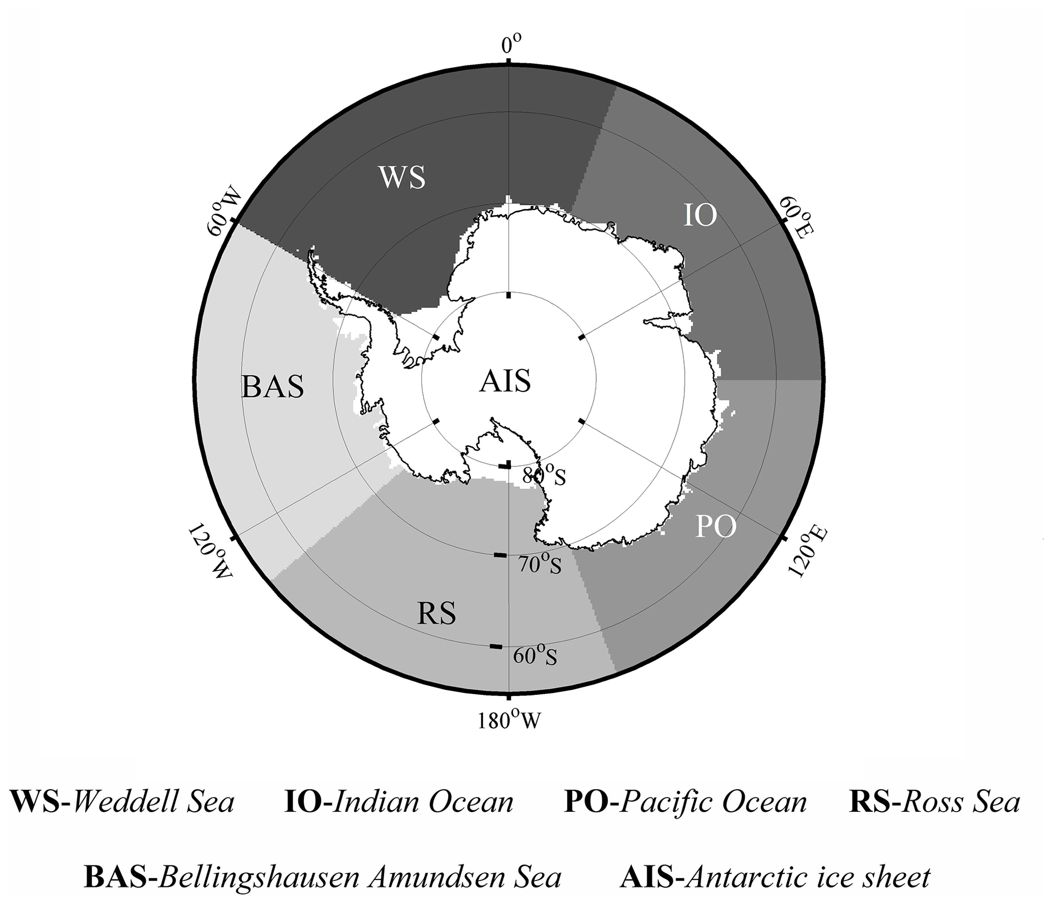
The study area includes the Southern Ocean and the Antarctic ice sheet and was divided into six sub-areas to investigate regional discrepancies in surface snowmelt on sea ice and the ice sheet according to Parkinson and Cavalieri (2012) (Fig. 1), namely the Weddell Sea (WS, 60∘ W to 20∘ E), Indian Ocean (IO, 20 to 90∘ E), Pacific Ocean (PO, 90 to 160∘ E), Ross Sea (RS, 160∘ E to 130∘ W), Bellingshausen and Amundsen seas (BAS, 130 to 60∘ W), and the AIS including all floating ice shelves.
3.1 Melt detection method
According to the Rayleigh–Jeans approximation, Tb is a function of emissivity (ε) and the near-surface physical temperature (Ts) of snow and ice (Zwally, 1977):
Tb varies greatly with the appearance and disappearance of snow liquid water (i.e., freeze–thaw cycle). The evolution of Tb with increasing liquid water can be divided into energy saturation and energy dampening phases. The initial increases in Tb are accompanied by the amplification of ε until the liquid water reaches a certain level. The subsequent energy dampening phase is characterized by monotonic decreases in Tb, which are caused by the increase in the snow–air interface reflectivity due to the amplified real part of the refractive index (Kang et al., 2014). Previous studies have emphasized the process by which Tb increases when snowpack starts to melt. However, Tb decreases after reaching a peak when the volumetric liquid water is approximately 1 % (Kang et al., 2014). The decline in Tb can also be caused by enhanced volume scattering as the snow grain size increases during the melt seasons. Single-channel methods may fail to work when the Tb of a melting snowpack is even lower than the winter mean in the late melt season due to energy dampening and snow metamorphism. Diurnal freeze–thaw cycles are prevalent in polar regions (Hall et al., 2009; Willmes et al., 2009; van den Broeke et al., 2010b). DAV shows very little variation in frozen seasons but is very sensitive to the diurnal freeze–thaw cycles throughout the melt seasons (Zheng et al., 2018).
A vertically polarized SSM/I 37 GHz DAV (DAV37) has been used in melt detection on the Greenland ice sheet and Antarctic sea ice (Willmes et al., 2006, 2009; Tedesco, 2007; Arndt et al., 2016). Extensive summer daily freeze–thaw cycles on the Antarctic sea-ice were found by SSM/I (Willmes et al., 2009). AMSR-E/2 has more opportunities to identify these transitions due to the more appropriate local acquisition time. AMSR-E/2 36.5 GHz DAV in vertical polarization (DAV36) was used to detect the pan-Antarctic region snowmelt and was calculated as follows:
where and are the in ascending and descending passes, respectively. Willmes et al. (2009) determined melt signals when the DAV37 of SSM/I exceed 10 K. The threshold was validated against extensive field data on the Antarctic sea ice. We utilized the same threshold for melt detection based on AMSR-E/2 DAV36 considering that the differences between AMSR-E 36 GHz Tb and SSM/I 37 GHz Tb are very small (Dai and Che, 2010). In the region south of 85∘ S where the surface snow is stable and never melts, the bias between the two measurements was only approximately 1 K for 2002–2003 (Fig. S1 in the Supplement). Slight Tb offsets between different sensors should not affect the results when using temporal Tb variability in melt detection (Markus et al., 2009).
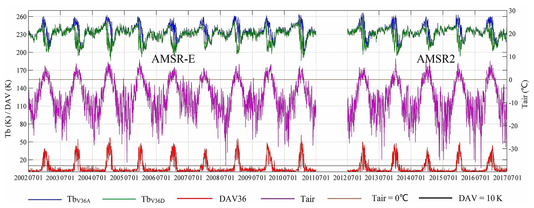
Figure 2The comparison between Tair and satellite observations (AMSR-E from 2002 to 2011 and AMSR2 from 2012 to 2017) at Zhongshan Station, including daily maximum Tair (purple line), (dark blue line), (dark green line) and DAV36 (red line); brown and black lines represent Tair = 0 ∘C and DAV = 10 K.
This method was also applied in the investigation of snow surface freeze–thaw cycles on the AIS. The verification of snowmelt is difficult, especially in the pan-Antarctic region where meltwater refreezes quickly and climatic data are sparse. However, surface snowmelt is determined by atmospheric conditions and agrees well with the Tair distribution pattern (Tedesco, 2007; Liang et al., 2013). In situ Tair measurements at Zhongshan Station (69.37∘ S, 76.38∘ E) obtained from the Chinese National Arctic and Antarctic Data Center (http://www.chinare.org.cn, last access: 1 March 2018) were used to evaluate the DAV36 algorithm (Fig. 2). The overall accuracy (p0, the proportion of observed agreement) and kappa coefficient were used to measure the coincidence based on the confusion matrix, where pc is the proportion in agreement due to chance (Cohen, 1960). and showed sharp increases at melt onset, while they decreased below the winter mean in the late melt seasons with associated snow metamorphism. However, positive maximum Tair agreed well with melt signals (i.e., the presence of liquid water) determined by the DAV method, with an overall accuracy of 0.93 and a Kappa coefficient of 0.79.
When a snowpack on sea ice begins to melt, it appears as a blackbody at microwave wavelengths and the Tb increases sharply (Markus et al., 2009), while open water exhibits a much lower Tb (Markus and Cavalieri, 1998). Therefore, Tb amplitudes may not be strong enough to be identified as melt signals for first-year sea ice with sufficient open water. To eliminate the effect of open water in melt detection, DAV36ice (i.e., DAV36 contributed by the ice-covered portion) was applied in the Antarctic sea ice snowmelt detection. Regardless of the atmospheric effects, the Tb of sea ice is comprised of the ice portion () and open-water portion () (Markus and Cavalieri, 1998):
Therefore, DAV36ice can be calculated as follows:
where SICA and SICD represent the SIC for the ascending and descending passes. If we assume that the SIC of the two passes remains unchanged (i.e., SICA=SICD), then we have
Figure 3 shows a comparison of meteorological observations for a sea ice buoy in the Weddell Sea and the corresponding AMSR2 measurements. Snow buoy observations (Fig. 3a), including snow depth and Tair, were obtained from the Alfred Wegener Institute (AWI, http://www.meereisportal.de/en/seaicemonitoring/buoy-mapsdata/, last access: 1 March 2018). The inset map in Fig. 3b illustrates the annual mean SIC and the route of the buoy from multiyear ice to first-year ice in the Weddell Sea. and showed great differences during the melt season. Sporadic melt events were detected before December 2014. Accompanied by a slight decrease in snow depth, DAV36 exceeded 10 K, and Tair went above the freezing point after mid-December. DAV36ice was nearly equal to DAV36 when SIC was above 90 %, while it was much higher than the latter when the SIC dropped after February. DAV36 was below 10 K with Tair above the freezing point many times (see the black arrows), while these melt signals were successfully recognized by the DAV36ice algorithm. The overall accuracy and kappa coefficient between the positive maximum Tair and melt signals derived by satellites were 0.79 and 0.50 based on the DAV36 algorithm, while those were 0.82 and 0.60 based on the DAV36ice algorithm, indicating a fair to good strength of agreement according to Fleiss et al. (2003). The DAV36ice algorithm performs better than the DAV36 algorithm in the marginal ice zone by reducing the effect of open water. We acknowledge that ice disintegrates and brine and flooding effects in the marginal sea ice zone may play an important role in Tb variations and obscure the DAVs (Smith, 1998; Willmes et al., 2009). The DAV method may fail to work when liquid water does not refreeze or when the snowpack is still melting during heavy melt seasons. The detection of snowmelt is sensitive to the threshold used in the DAV method. A lower (higher) threshold will result in generally more (less) satellite-based melt signals.
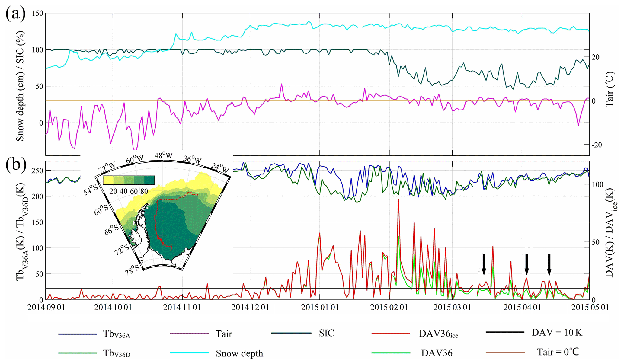
Figure 3Meteorological and satellite measurements along a sea ice buoy in the Weddell Sea from 1 September 2014 to 1 May 2015. (a) Snow depth (cyan line), daily maximum Tair (pink line) and SIC (olive line); the brown line represents . (b) (dark blue line), (dark green line), DAV36 (light green line) and DAV36ice (red line); the black line represents DAV = 10 K. The inset map in (b) illustrates the annual mean SIC and the route of the buoy from multiyear ice to first-year ice. The black arrows indicate the cases in which melt events were recognized by DAV36ice rather than DAV36.
Melt signals derived from the DAV method and the positive Tair from the automatic weather station (AWS) were not always strictly connected (Figs. 1 and 2). The mismatches largely occur in the period with transient snowmelt when thaw–freeze status shifted quickly and in the regions with plenty of open water (typical SIC < 90 %). For the periods that were identified as having a thaw–freeze status for at least 3 d, satellite-derived melt signals showed close agreement (OA=0.87, Kappa=0.68) with those derived from Tair over the sea ice with SIC > 90 %. Disagreements in the identification of transient melt events may result from inconsistent spatial and temporal resolutions. Validating the large-scale satellite-based estimation (25 km for AMSR-E/2) against station-based measurements is always challenging due to representativeness errors (Lyu et al., 2017). The daily maximum Tair was derived from hourly Tair records, while only two daily satellite observations were used in the DAV method. In addition, snowmelt may occur when Tair is below the freezing point because of the penetration and absorption of solar radiation within the snowpack (Koh and Jordan, 1995). Markus et al. (2009) determined the Arctic sea ice freeze–thaw states based on a gridded Tair data set with a threshold of −1 ∘C. Melt timing derived from different approaches is supposed to show similar spatial distribution patterns. To evaluate the performance of the DAV method on a larger scale, snowmelt over the pan-Antarctic region was also determined by ERA-Interim reanalysis when the daily maximum Tair exceeded −1 ∘C.
Considering the existence of both transient and persistent snowmelt in the pan-Antarctic region, early melt onset (EMO, the first day when snowmelt is detected) and continuous melt onset (CMO, the first day when snowmelt lasts for at least 3 consecutive days) were investigated in this study. Melting days were calculated by summing the number of days with snowmelt. Sufficient Antarctic sea ice melts quickly in austral summer and does not emerge again in the melting year. In such cases, the last day of snowmelt is always the day that the SIC drops below 15 %, rather than the day that freeze-up begins. Thus, freeze-up and melt duration were not included in this study. Antarctic sea ice cover has exhibited considerable regional and annual variations (Hobbs et al., 2016). To be consistent, the melting day fraction (MDF) and melt extent fraction (MEF) were introduced to study the snowmelt variations:
where ice cover was determined with a SIC > 15 % for sea ice, and the AIS is assumed to be ice-covered all year.
Table 1Annual mean and standard deviation of pan-Antarctic region EMO, CMO, melting days and MDF derived by AMSR-E/2 and ERA-Interim.

3.2 Data preprocessing and analysis
To capture complete melt seasons, a melting year begins on 1 July and ends on 30 June of the next year. The missing observations were filled based on timeline interpolation. Spurious Tb variations may occasionally be mistaken for melt signals, which can be caused by clouds, atmospheric water vapor, wind-induced surface roughening, and residual calibration errors. To mitigate their impacts on melt detection, a median spatial filter with a 3×3 window was applied to the satellite observations. Furthermore, melt detection was constrained to the days with compatible thermal regimes following Belchansky et al. (2004). The days with ERA-Interim ∘C were first determined, and the DAV36 algorithm was applied henceforth. Linear trends were calculated using a least-squares method. The significance levels of the correlations and regressions were determined using the Student t tests.
To study the response of the pan-Antarctic region surface snowmelt to circulation conditions, we explored the relationship between the melt indices and El Niño–Southern Oscillation (ENSO) and Southern Annular Mode (SAM). Nino3.4, the average sea surface temperature anomaly in the tropics (5∘ S–5∘ N, 170–120∘ W), is calculated from the Hadley Centre Sea Ice and Sea Surface Temperature data set (Rayner et al., 2003). The Southern Oscillation Index (SOI) is calculated using the pressure difference between Tahiti and Darwin (Ropelewski et al., 1987). The SAM is calculated using the zonal pressure difference between 40 and 65∘ S (Marshall, 2003).
4.1 Snowmelt distribution and trends
Integrated pan-Antarctic region annual melt indices were examined based on AMSR-E/2 (Fig. 4a–d). The CMO ranges from August in the marginal sea ice zone to January in the Antarctic inland, and the pan-Antarctic region EMO arrived 53 d earlier on average (Table 1). In general, snowmelt shows significant latitudinal zonality. The EMO and CMO occur later from the marginal sea ice to the inland of the AIS, from low latitudes to high latitudes, while the MDF increases in the opposite direction.
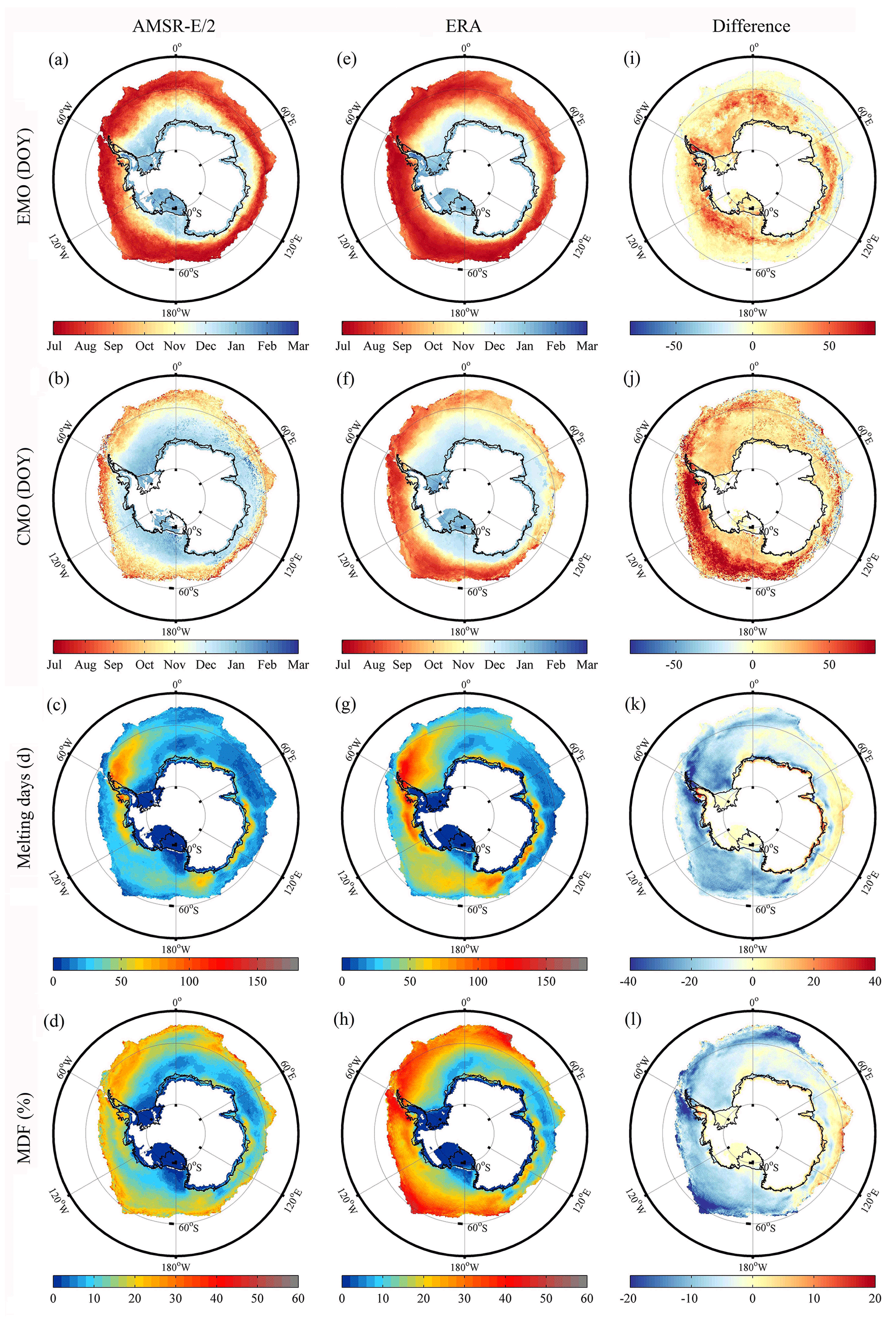
Figure 4Annual mean EMO, CMO, melting days and MDF derived by AMSR-E/2 (a–d) and ERA-Interim (e–h). Also shown are the differences (AMSR-E/2 minus ERA-Interim) between the two observations (i–l).
The annual mean EMO, CMO, melting days and MDF of the six sub-areas were also analyzed (Table 1). In terms of the satellite observations, the earliest EMO (15 August) and CMO (5 November) occurred in the BAS, where surface snow melted for 37 d. As expected, snowmelt on the AIS had the latest onset, with EMO occurring on 7 December and CMO occurring on 18 December. Sea ice surface snow in the WS can melt for more than 100 d (Fig. 4c). MDF can reach 30 % for the marginal sea ice in the RS and WS (Fig. 4d). Snowmelt at high latitudes was variable. For example, surface snowmelt on the Ross Ice Shelf extended to the inland area and even reached the Transantarctic Mountains in 2004/05, but the Ross Ice Shelf was almost totally frozen during 2009–2011 (not shown).
Melting timing derived from AMSR-E/2 satellite observations and ERA-Interim reanalysis generally agreed well with each other in the AIS and IO but showed some discrepancies in other regions (Table 1 and Fig. 4). On average, the pan-Antarctic region EMO and CMO derived by satellites were 11 and 27 d later than those detected by ERA-Interim. AMSR-E/2 detected later EMO on the near-shore sea ice and later CMO in the BAS and RS (Fig. 4i and j). ERA-Interim recognized more melt events in the WS (16 d), BAS (19 d) and RS (20 d), where intense surface snowmelt was found (Fig. 4k). The satellite-based MDF for the marginal sea ice is lower than that derived by ERA-Interim (Fig. 4l). With the exception of the Antarctic Peninsula, where the melt season can last for more than 3 months, the AIS melt timings detected by the two methods were consistent with each other (Fig. 4i–l).
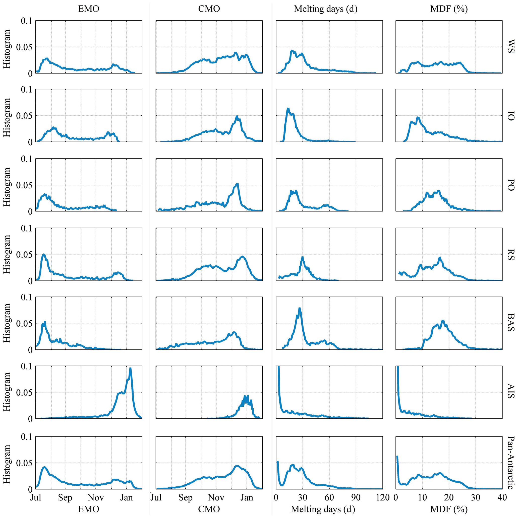
Figure 5Normalized histograms of annual mean EMO, CMO, melting days and MDF for the pan-Antarctic region and different regions.
The seasonal evolution of snowmelt in different regions was examined by the normalized histograms of annual mean EMO, CMO, melting days and MDF (Fig. 5). Notable differences existed between the temporal distribution of sea ice and ice sheet melt patterns. Sea ice EMO peaked in mid-July in the BAS and in early August for IO. By contrast, the frequency of AIS EMO did not reach the peak until early January. The occurrence of pan-Antarctic region CMO peaked in December, varying from early December in the BAS and WS to late December in the AIS. Melting days and MDF histograms indicate a large number of transient melt events, especially in the AIS. Approximately 16 % of the AIS experienced snowmelt during 2002–2017; however, approximately 66 % of these areas melted for no more than 5 d. In general, melting days seldom exceeded 45 d, with the exception of the BAS and WS where plenty of surface snow on sea ice can melt for more than 2 months. The annual mean MDF in the BAS was 17 % (Table 1), while the MDF in most of the AIS was below 5 % (Fig. 5).
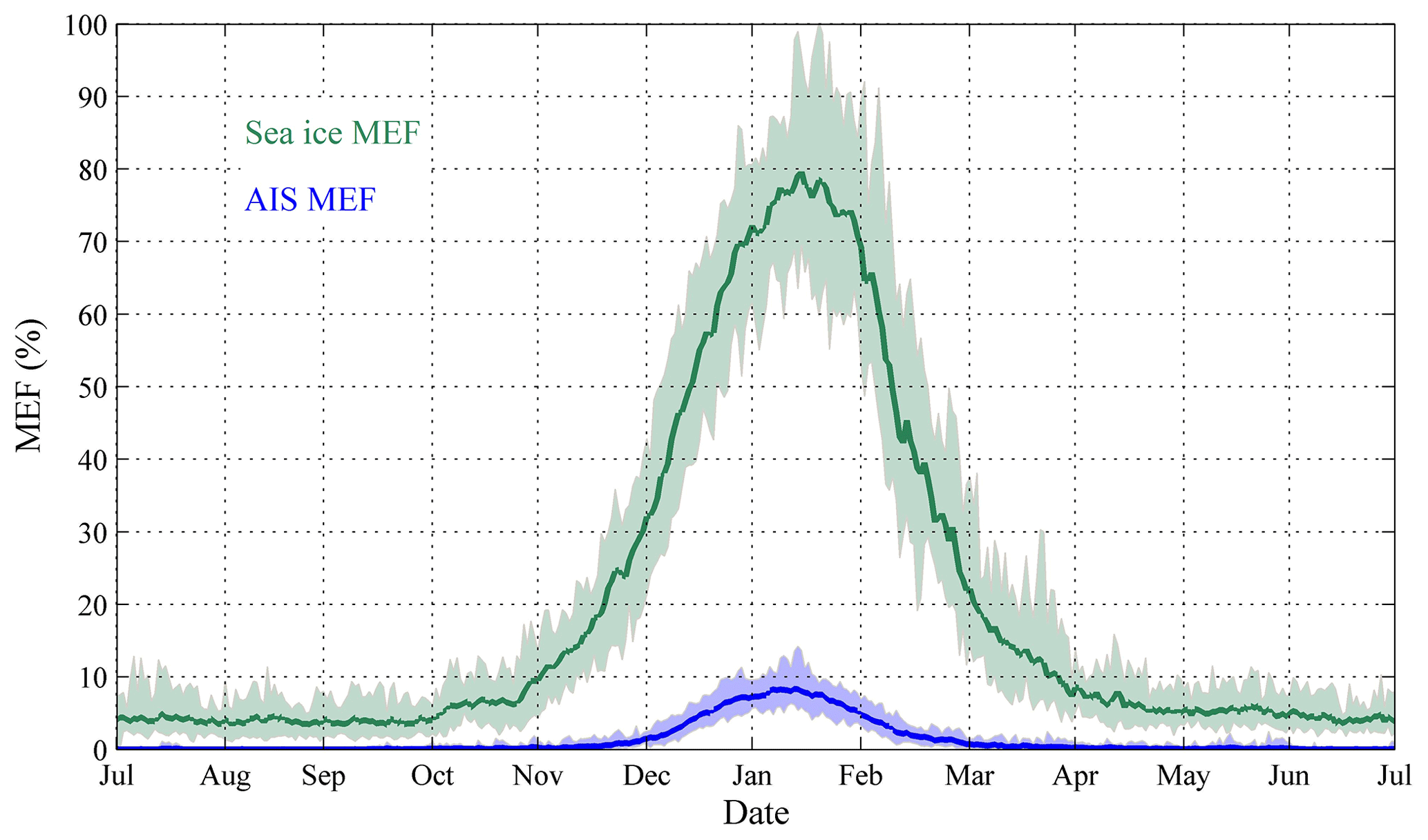
Figure 6Daily mean Antarctic sea ice MEF and AIS MEF; the corresponding shadows indicate daily maxima and minima.
The CMO histogram suggests that most of the pan-Antarctic region continuous snowmelt began between October and January (Fig. 5), corresponding to a sharp increase in MEF (Fig. 6). In mid-January, most of the Antarctic sea ice experienced surface snowmelt, and the daily mean MEF can reach 80 %. The AIS daily mean MEF was much lower and reached a maximum (8 %) in mid-January (Fig. 6). The MEF declined rapidly between late January and March. The Antarctic sea ice daily mean MEF declined to below 10 %, and the AIS became almost completely refrozen after April.

Figure 7Trends in (a) CMO, (b) melting days and (c) MDF; black points indicate the pixels with trends above the 90 % confidence level.
Trends in surface melting conditions for 2002–2017 were analyzed. Linear trends for the pixels with continuous records were calculated based on the annual departures. EMO is not included in the trend analysis because of the chaotic spatial distribution of the early transient melt events. A considerable decrease in surface snowmelt in the RS can be clearly seen in Fig. 7, which illustrates the trends in melt indices during 2002–2017. No significant CMO trend was observed in most of the pan-Antarctic region. Melting days and MDF for the offshore sea ice in the RS presented remarkable negative trends. Surface snow on the East Antarctic sea ice, especially in PO, presented trends towards increasing melting days and MDF. CMO appeared earlier on the WS marginal sea ice, where melting days and MDF also significantly increased. Many low-lying ice shelves in the AIS, such as the Larsen C Ice Shelf on the Antarctic Peninsula and the Abbot Ice Shelf in Marie Byrd Land, presented trends towards decreasing melting days and MDF.
4.2 Linkages between pan-Antarctic region surface snowmelt and climate indices
Snowmelt in the pan-Antarctic region was found to be strongly associated with ENSO and SAM (Turner, 2004; Tedesco and Monaghan, 2009; Oza et al., 2011; Meredith et al., 2017). In January 2016, the extensive surface snowmelt in West Antarctica was likely linked with sustained and strong advection of warm marine air due to the concurrent strong El Niño event (Nicolas et al., 2017). The weakly negative trend in surface temperature in Antarctica was consistent with the positive trends in SAM during summer and autumn since the 1970s (Monaghan et al., 2008).
Table 2Correlation between snowmelt index and climate index for the period 2002–2017.
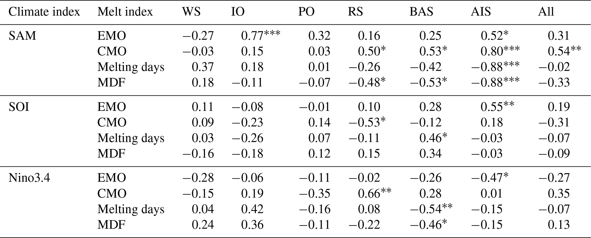
Correlation coefficients with *, and indicate statistical significance at 90 %, 95 % and 99 % confidence levels, respectively.
The comparisons between pan-Antarctic region surface snowmelt and the climate indices are illustrated in Table 2. The CMO of the pan-Antarctic region was significantly correlated (at the 95 % confidence level) with summer (DJF) SAM. CMO and MDF were also well correlated with the summer SAM in the RS, BAS and AIS. The correlation coefficient between EMO and SAM was the highest (0.77) in the IO. CMO was significantly correlated with the SOI and Nino3.4 in the RS. Melting days and MDF were also found to be strongly correlated with the summer SOI or Nino3.4 in the BAS where strong decreases in sea ice concentration and duration were always linked with contemporary ENSO warm events (Kwok et al., 2002; Bromwich et al., 2004).
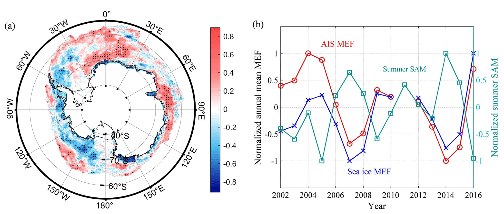
Figure 8Linkage between pan-Antarctic region snowmelt and summer SAM. (a) Correlation coefficient between MDF and summer SAM; black points indicate the trends above the 90 % confidence level. (b) Comparison of normalized summer SAM (cyan line), normalized annual mean Antarctic sea ice MEF (blue line) and AIS MEF (red line).
The MDF was negatively related to the summer SAM for offshore sea ice in the BAS and RS where the MDF has significantly decreased (Fig. 8). This relationship was especially significant in the AIS (, P<0.01). High anti-correlations were found between the summer SAM and the annual mean MEF on the Antarctic sea ice and AIS (Fig. 8b). The significantly decreased (at the 95 % confidence level) annual mean melt extent on the AIS ( km2 yr−1) for 2002–2017 was strongly associated with increasing summer SAM (, P<0.01). This phenomenon is in line with the decreased surface snowmelt and the enhanced summer SAM in the AIS since the 1970s (Marshall, 2003; Tedesco and Monaghan, 2009). The positive SAM results in anomalously strong westerlies over the Southern Ocean and hence the reduction in poleward heat transport, leading to the subsequent atmospheric cooling in the Antarctic regions (Thompson and Solomon, 2002). The SAM is the principal driver of AIS near-surface temperature and snowmelt variability (Marshall, 2007; Tedesco and Monaghan, 2009). The SAM is expected to have a continuous effect on the Antarctic climate in the next few decades considering the projected ozone recovery (Thompson et al., 2011).
5.1 Comparisons
Tair above or below the freezing point does not always indicate a melting or frozen snowpack. The EMO and CMO derived from ERA-Interim were earlier than those detected by AMSR-E/2 data (Fig. 4 and Table 1). This is because it takes time to produce liquid water when snow temperature approaches the melting point. Daily Tb variation is limited when liquid water does not refreeze or snowpack is still melting in warm nights during heavy-melt seasons (Willmes et al., 2009; Semmens and Ramage, 2014). As a result, ERA-Interim recognized more melt events for the regions where heavy snowmelt was found and the DAV method fails to work, such as the WS, BAS, RS and the Larsen C ice shelf. This might also be the reason that the melt onset was very early in the RS while few melt events were detected by AMSR-E/2. This is also one of the reasons that AMSR-E/2 melt signals do not strictly agree with AWS positive Tair and is considered the key limitation of the DAV method.
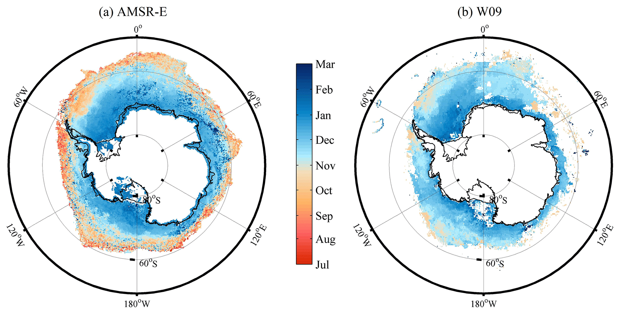
Figure 9Annual mean CMO derived from (a) AMSR-E and (b) W09 from 2002 to 2008.
Willmes et al. (2009) established the SSM/I DAV method to study the Antarctic sea ice CMO (hereafter W09). Antarctic sea ice CMO mapped by AMSR-E shows a higher spatial continuity than that in W09. The CMO dates derived from the two satellites agreed well with each other at high latitudes for 2002–2008. However, W09 found a remarkably later CMO on the marginal sea ice compared with the results from AMSR-E (Fig. 9). There are several reasons for the significant difference in marginal sea ice CMO detected by AMSR-E and SSM/I data. First, W09 only studied surface snowmelt on sea ice after 1 October, while the melt season begins on 1 July in this study. Second, the DAV36ice algorithm can amplify snowmelt signals by reducing the effect of open water, so that more melt events can be recognized (Fig. 3). Third, compared with SSM/I, AMSR-E operated in a stable orbit and observed the pan-Antarctic region with a more appropriate local acquisition time and hence had more opportunities to identify melt events (Fig. S2 in the Supplement).
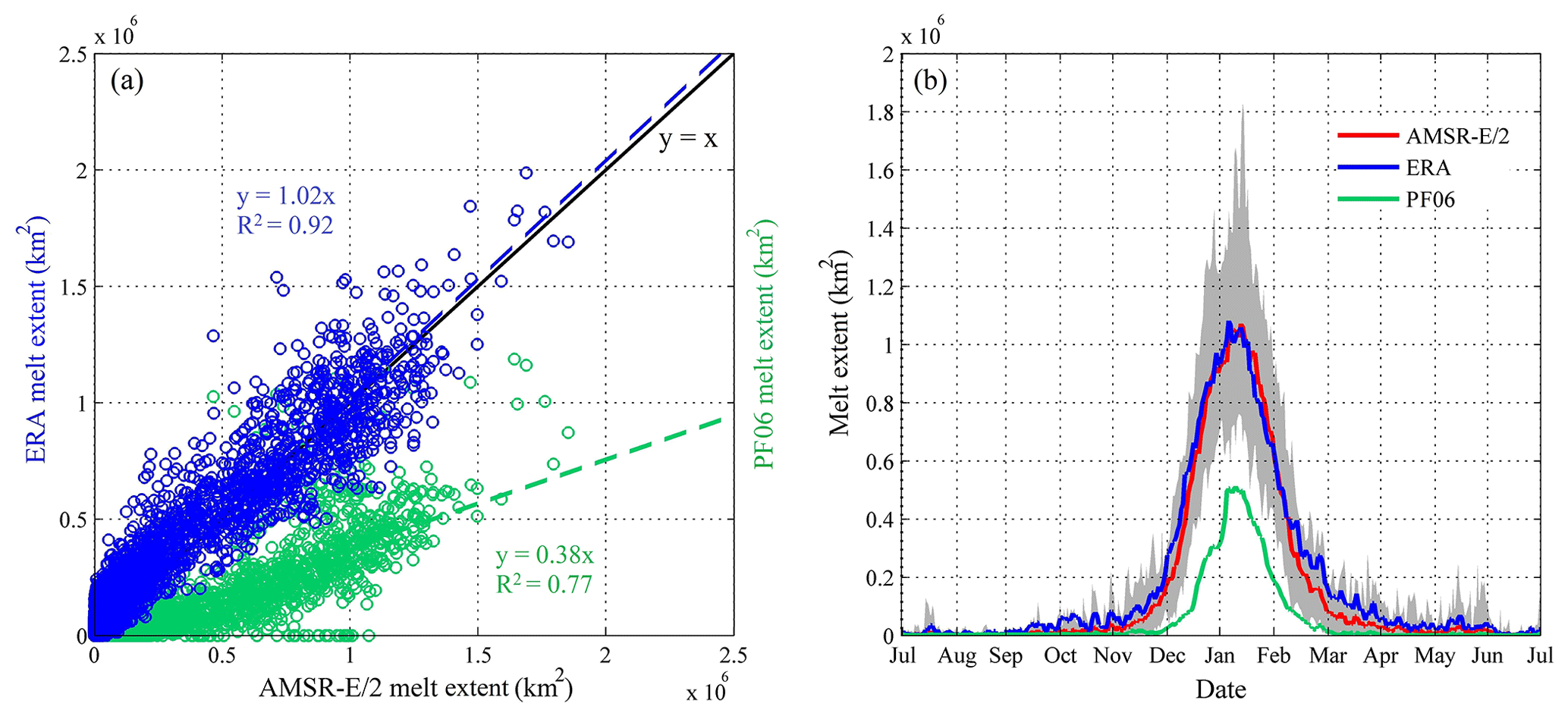
Figure 10Comparison of AIS melt extent derived by AMSR-E/2, ERA-Interim and PF06 from 2002 to 2017. (a) Scatter plot of daily melt extent; blue circles indicate AMSR-E/2 vs. ERA-Interim and green circles indicate AMSR-E/2 vs. PF06. (b) Daily mean melt extent derived by AMSR-E/2 (red line), ERA-Interim (blue line) and PF06 (green line); grey shading indicates the daily maximum and minimum melt extent detected by AMSR-E/2.

Figure 11Annual mean EMO (blue dots), CMO (black dots), melting days (cyan dots) and MDF (red dots) with the threshold for AMSR-E/2 DAV36 varying from 6 to 14 K.
Considering that snowmelt can be biased by various SMMR and SSM/I acquisition times, Picard and Fily (2006) retrieved the AIS surface snowmelt based on corrected 18–19 GHz Tb time series (hereafter PF06). The AIS daily melt extents derived by AMSR-E/2 and ERA-Interim were consistent with each other (R2=0.92). The PF06 daily melt extent also presented a high correlation with the results from AMSR-E/2 (R2=0.77). However, the melt extent derived by PF06 was significantly smaller than that mapped by AMSR-E/2 (Fig. 10a). AMSR-E/2 and ERA-Interim daily mean melt extents were more than twice the melt extent mapped by PF06 from December to February (Fig. 10b). In a recent study, the PF06 melt extent was also found to be much smaller than that derived from scatterometers (Zheng et al., 2020). PF06 determined snowmelt when the SSM/I 19 GHz Tb exceeds the winter mean plus 2.5 times the standard deviation of the winter Tb. During the melt seasons, Tb may decrease due to the strong volume scattering resulting from the increase in snow grain size and the formation of icy layers (Ramage and Isacks, 2002; Markus et al., 2009). Summer Tb can even be much lower than the winter observations (Zheng et al., 2018). Therefore, PF06 may underestimate surface snowmelt when snow metamorphism occurs during the melt season. The DAV method is unaffected by snow metamorphism but may fail to work when liquid water does not refreeze or snowpack is still melting during warm nights (Willmes et al., 2009). Fortunately, the Antarctic surface snowmelt is always short-lived and can refreeze quasi-instantaneously (Zheng et al., 2018; van den Broeke et al., 2010a).
5.2 Uncertainties
There are several uncertainties in the pan-Antarctic region snowmelt derived from AMSR-E/2 data. First, the regions with snowmelt that became more prevalent would presumably show a decrease in melting days based on the DAV method when snowmelt even occurs at night. Second, although the DAV method used in this study performs well when compared with meteorological observations, the optimal threshold may differ temporally and regionally with varying snow properties. Arndt et al. (2016) utilized individual local thresholds with a median value of 6 K to detect snowmelt based on SSM/I DAV and recognized an earlier melt onset than W09. Melt indices derived from the DAV method show considerable variations when applying different thresholds (from 6 to 14 K in Fig. 11). Varying the threshold applied to AMSR-E/2 DAV by ±4 K results in −17 to 14 d of departure for the annual mean EMO and −9 to 12 d of departure for annual mean melting days.
It should be noted that the presence of snow liquid water detected by the AMSR-E/2 DAV method does not necessarily mean that the melt energy is positive because it takes time for meltwater to refreeze. In addition, after the refreezing of surface snow, subsurface liquid water can still be detected by a radiometer due to the penetrating capacity of microwaves (Ashcraft and Long, 2006). We detect snowmelt with AMSR-E/2, while using a SIC product generated by different sensors (SMMR and SSM/I) that observe the pan-Antarctic regions at different acquisition times. The DAV36ice algorithm for sea ice snowmelt detection assumes that the SIC of the two passes remains unchanged, which may not be true and may lead to misidentifications of melt signals due to quick sea ice drift and disintegration. The algorithm can be further improved if the twice-daily AMSR-E/2 SIC product is available in the future. Although AMSR-E/2 observed the pan-Antarctic region at the appropriate times for snowmelt detection, they may underestimate snowmelt because snowmelt can occur at any time and refreezing can be quasi-instantaneous. Other sources of the microwave remote sensing data set, such as scatterometers and synthetic aperture radar, are expected to enrich daily observations in future works.
In this study, we investigated the pan-Antarctic region surface melting conditions for 2002–2017 by using daily AMSR-E/2 observations. The more stable orbits and more appropriate local acquisition times of AMSR-E/2 compared to those of SSM/I enabled us to take full advantage of the brightness temperature variations to investigate surface melt events. The performance of this method was improved in the marginal sea ice zone by excluding the effect of open water. Although this method may fail to recognize melt events when meltwater does not refreeze or snowpack melts during warm nights, snowmelt detected by AMSR-E/2 agreed well with the in situ positive Tair observations and was more extensive than that detected by SSM/I.
Pan-Antarctic region snowmelt showed significant latitudinal zonality. Continuous melt onset (CMO) ranges from August in the marginal sea ice zone to January in the Antarctic inland. Snowmelt on the Antarctic sea ice and Antarctic ice sheet exhibited great differences in temporal distribution patterns. Sea ice in the Weddell Sea can melt for more than 100 d while snowmelt seldom occurs in the Antarctic inland. Negative trends in snowmelt were found in the Ross Sea and Antarctic ice sheet. The pan-Antarctic region CMO was well correlated with the summer Southern Annular Mode. The decreasing surface snowmelt in the Antarctic ice sheet was very likely linked with the positive summer Southern Annular Mode during 2002–2017.
The Southern Hemipshere AMSR-E and AMSR2 data were obtained from the National Snow and Ice Data Center (NSIDC, https://nsidc.org/data/nsidc-0301, last access: 20 January 2018, Knowles et al., 2006) and the Japan Aerospace Exploration Agency (JAXA, https://suzaku.eorc.jaxa.jp/GCOM_W/data/data_w_index.html, last access: 20 January 2018, Imaoka et al., 2010). The bootstrap sea ice concentration data were also provided by NSIDC (http://nsidc.org/data/nsidc-0079, last access: 20 January 2018, Comiso, 2017). The ERA-Interim reanalysis is available from the European Centre for Medium-Range Weather Forecasts (ECMWF, https://apps.ecmwf.int/datasets/data/interim-full-daily/levtype=sfc/, last access: 15 February 2018, Dee et al., 2011).
The supplement related to this article is available online at: https://doi.org/10.5194/tc-14-3811-2020-supplement.
LZ, CZ and TZ conceived the study. CZ and TZ provided primary support and guidance on the research. LZ developed and processed the satellite-derived melt data with assistance from QL and KW and led the writing of the manuscript. All authors provided valuable insights and contributed to the final version of the manuscript.
The authors declare that they have no conflict of interest.
We would like to express our gratitude to the editor and reviewers for their careful and insightful comments. The numerical calculations in this paper have been done on the supercomputing system in the Supercomputing Center of Wuhan University. This research was funded by the National Natural Science Foundation of China (NSFC) and the Funds for the Distinguished Young Scientists of Hubei Province (China).
This research has been supported by the National Natural Science Foundation of China (NSFC) (grant nos. 41776200, 41941010 and 41531069) and the Funds for the Distinguished Young Scientists of Hubei Province (China) (grant no. 2019CFA057).
This paper was edited by Stef Lhermitte and reviewed by two anonymous referees.
Abdalati, W. and Steffen, K.: Passive microwave-derived snow melt regions on the Greenland Ice Sheet, Geophys. Res. Lett., 22, 787–790, https://doi.org/10.1029/95GL00433, 1995.
Ackley, S. F., Lewis, M. J., Fritsen, C. H., and Xie, H.: Internal melting in Antarctic sea ice: Development of “gap layers”, Geophys. Res. Lett., 35, L11503, https://doi.org/10.1029/2008GL033644, 2008.
Arndt, S., Willmes, S., Dierking, W., and Nicolaus, M.: Timing and regional patterns of snowmelt on Antarctic sea ice from passive microwave satellite observations, J. Geophys. Res.-Oceans, 121, 5916–5930, https://doi.org/10.1002/2015JC011504, 2016.
Ashcraft, I. S. and Long, D. G.: Comparison of methods for melt detection over Greenland using active and passive microwave measurements, Int. J. Remote Sens., 27, 2469–2488, https://doi.org/10.1080/01431160500534465, 2006.
Belchansky, G. I., Douglas, D. C., and Platonov, N. G.: Duration of the Arctic sea ice melt season: Regional and interannual variability, 1979–2001, J. Climate, 17, 67–80, https://doi.org/10.1175/1520-0442(2004)017{<}0067:DOTASI{>}2.0.CO;2, 2004.
Bell, R. E., Banwell, A. F., Trusel, L. D., and Kingslake, J.: Antarctic surface hydrology and impacts on ice-sheet mass balance, Nat. Clim. Change, 8, 1044–1052, https://doi.org/10.1038/s41558-018-0326-3, 2018.
Brandt, R. E., Warren, S. G., Worby, A. P., and Grenfell, T. C.: Surface albedo of the Antarctic sea ice zone, J. Climate, 18, 3606–3622, https://doi.org/10.1175/JCLI3489.1, 2005.
Bromwich, D. H., Monaghan, A. J., and Guo, Z.: Modeling the ENSO modulation of Antarctic climate in the late 1990s with the Polar MM5, J. Climate, 17, 109–132, https://doi.org/10.1175/1520-0442(2004)017{<}0109:MTEMOA{>}2.0.CO;2, 2004.
Cohen, J.: A Coefficient of Agreement for Nominal Scales, Educ. Psychol. Meas., 20, 37–46, https://doi.org/10.1177/001316446002000104, 1960.
Comiso, J.: Bootstrap Sea Ice Concentrations from Nimbus-7 SMMR and DMSP SSM/I-SSMIS, Version 3, NASA National Snow and Ice Data Center Distributed Active Archive Center, NSIDC, Boulder, Colorado, USA, https://doi.org/10.5067/7Q8HCCWS4I0R, 2017.
Comiso, J. C. and Nishio, F.: Trends in the sea ice cover using enhanced and compatible AMSR-E, SSM/I, and SMMR data, J. Geophys. Res., 113, C02S07, https://doi.org/10.1029/2007JC004257, 2008.
Dai, L. and Che, T.: Cross-platform calibration of SMMR, SSM/I and AMSR-E passive microwave brightness temperature, Sixth Int. Symp. Digit. Earth Data Process. Appl., 7841, 784103, https://doi.org/10.1117/12.873150, 2010.
Dee, D. P., Uppala, S. M., Simmons, A. J., Berrisford, P., Poli, P., Kobayashi, S., Andrae, U., Balmaseda, M. A., Balsamo, G., Bauer, P., Bechtold, P., Beljaars, A. C. M., van de Berg, L., Bidlot, J., Bormann, N., Delsol, C., Dragani, R., Fuentes, M., Geer, A. J., Haimberger, L., Healy, S. B., Hersbach, H., Hólm, E. V., Isaksen, L., Kållberg, P., Köhler, M., Matricardi, M., McNally, A. P., Monge-Sanz, B. M., Morcrette, J.-J., Park, B.-K., Peubey, C., de Rosnay, P., Tavolato, C., Thépaut, J.-N., and Vitart, F.: The ERA-Interim reanalysis: configuration and performance of the data assimilation system, Q. J. Roy. Meteor. Soc., 137, 553–597, https://doi.org/10.1002/qj.828, 2011.
Drinkwater, M. R. and Liu, X.: Seasonal to interannual variability in Antarctic sea-ice surface melt, IEEE T. Geosci. Remote, 38, 1827–1842, https://doi.org/10.1109/36.851767, 2000.
Fleiss, J. L., Levin, B., and Paik, M. C.: Statistical Methods for Rates and Proportions, 3rd edn., Wiley, Hoboken, New Jersey, 604 pp., 2003.
Hall, D. K., Nghiem, S. V., Schaaf, C. B., DiGirolamo, N. E., and Neumann, G.: Evaluation of surface and near-surface melt characteristics on the Greenland ice sheet using MODIS and QuikSCAT data, J. Geophys. Res.-Earth, 114, F04006, https://doi.org/10.1029/2009JF001287, 2009.
Hobbs, W. R., Massom, R., Stammerjohn, S., Reid, P., Williams, G., and Meier, W.: A review of recent changes in Southern Ocean sea ice, their drivers and forcings, Global Planet. Change, 143, 228–250, https://doi.org/10.1016/J.GLOPLACHA.2016.06.008, 2016.
Imaoka, K., Kachi, M., Fujii, H., Murakami, H., Hori, M., Ono, A., Igarashi, T., Nakagawa, K., Oki, T., Honda, Y., and Shimoda, H.: Global change observation mission (GCOM) for monitoring carbon, water cycles, and climate change, Proc. IEEE, 98, 717–734, https://doi.org/10.1109/JPROC.2009.2036869, 2010.
Intergovernmental Panel on Climate Change (IPCC): Climate change 2013: the physical science basis. Fifth assessment report of the intergovernmental panel on climate change, Cambridge Univ. Press, Cambridge, UK, 2014.
Joshi, M., Merry, C. J., Jezek, K. C., and Bolzan, J. F.: An edge detection technique to estimate melt duration, season and melt extent on the Greenland Ice Sheet using Passive Microwave Data, Geophys. Res. Lett., 28, 3497–3500, https://doi.org/10.1029/2000gl012503, 2001.
Kang, D. H., Barros, A. P., and Dery, S. J.: Evaluating Passive Microwave Radiometry for the Dynamical Transition From Dry to Wet Snowpacks, IEEE T. Geosci. Remote, 52, 3–15, 2014.
Knowles, K., Savoie, M., Armstrong, R., and Brodzik, M. J.: AMSR-E/Aqua Daily EASE-Grid Brightness Temperatures, Version 1, Southern Hemisphere, Boulder, Colorado USA, NASA National Snow and Ice Data Center Distributed Active Archive Center, https://doi.org/10.5067/XIMNXRTQVMOX (last access: 20 January 2018), 2006.
Koh, G. and Jordan, R.: Sub-surface melting in a seasonal snow cover, J. Glaciol., 41, 474–482, https://doi.org/10.3189/S002214300003481X, 1995.
Kwok, R., Comiso, J. C., Kwok, R., and Comiso, J. C.: Southern Ocean Climate and Sea Ice Anomalies Associated with the Southern Oscillation, J. Climate, 15, 487–501, https://doi.org/10.1175/1520-0442(2002)015{<}0487:SOCASI{>}2.0.CO;2, 2002.
Liang, L., Guo, H., Li, X., and Cheng, X.: Automated ice-sheet snowmelt detection using microwave radiometer measurements, Polar Res., 32, 1–13, https://doi.org/10.3402/polar.v32i0.19746, 2013.
Liu, H., Wang, L., and Jezek, K. C.: Wavelet-transform based edge detection approach to derivation of snowmelt onset, end and duration from satellite passive microwave measurements, Int. J. Remote Sens., 26, 4639–4660, https://doi.org/10.1080/01431160500213342, 2005.
Lyu, H., Mccoll, K. A., Li, X., Derksen, C., Berg, A., Black, T. A., Euskirchen, E., Loranty, M., Pulliainen, J., Rautiainen, K., Rowlandson, T., Roy, A., Royer, A., Langlois, A., Stephens, J., Lu, H., and Entekhabi, D.: Validation of the SMAP freeze/thaw product using categorical triple collocation, Remote Sens. Environ., 205, 329–337, https://doi.org/10.1016/j.rse.2017.12.007, 2017.
Markus, T. and Cavalieri, D. J.: Snow Depth Distribution Over Sea Ice in the Southern Ocean from Satellite Passive Microwave Data, in: Antarctic Sea Ice: Physical Processes, Interactions and Variability, Vol. 74, 19–39, American Geophysical Union, Washington, DC, USA, 1998.
Markus, T., Stroeve, J. C., and Miller, J.: Recent changes in Arctic sea ice melt onset, freezeup, and melt season length, J. Geophys. Res.-Oceans, 114, C12024, https://doi.org/10.1029/2009JC005436, 2009.
Marshall, G. J.: Trends in the Southern Annular Mode from observations and reanalyses, J. Climate, 16, 4134–4143, https://doi.org/10.1175/1520-0442(2003)016{<}4134:TITSAM{>}2.0.CO;2, 2003.
Marshall, G. J.: Half-century seasonal relationships between the Southern Annular Mode and Antarctic temperatures, Int. J. Climatol., 27, 373–383, https://doi.org/10.1002/joc.1407, 2007.
Meier, W. N. and Stroeve, J.: Comparison of sea-ice extent and ice-edge location estimates from passive microwave and enhanced-resolution scatterometer data, Ann. Glaciol., 48, 65–70, https://doi.org/10.3189/172756408784700743, 2008.
Meredith, M. P., Stammerjohn, S. E., Venables, H. J., Ducklow, H. W., Martinson, D. G., Iannuzzi, R. A., Leng, M. J., van Wessem, J. M., Reijmer, C. H., and Barrand, N. E.: Changing distributions of sea ice melt and meteoric water west of the Antarctic Peninsula, Deep-Sea Res. Pt. II, 139, 40–57, https://doi.org/10.1016/j.dsr2.2016.04.019, 2017.
Monaghan, A. J., Bromwich, D. H., Chapman, W., and Comiso, J. C.: Recent variability and trends of Antarctic near-surface temperature, J. Geophys. Res.-Atmos., 113, D04105, https://doi.org/10.1029/2007JD009094, 2008.
Mote, T. L. and Anderson, M. R.: Variations in snowpack melt on the Greenland ice sheet based on passive-microwave measurements, J. Glaciol., 41, 51–60, 1995.
Nicolas, J. P., Vogelmann, A. M., Scott, R. C., Wilson, A. B., Cadeddu, M. P., Bromwich, D. H., Verlinde, J., Lubin, D., Russell, L. M., Jenkinson, C., Powers, H. H., Ryczek, M., Stone, G., and Wille, J. D.: January 2016 extensive summer melt in West Antarctica favoured by strong El Niño, Nat. Commun., 8, 15799, https://doi.org/10.1038/ncomms15799, 2017.
Oza, S. R., Singh, R. K. K., Vyas, N. K., and Sarkar, A.: Study of inter-annual variations in surface melting over Amery Ice Shelf, East Antarctica, using space-borne scatterometer data, J. Earth Syst. Sci., 120, 329–336, 2011.
Parkinson, C. L. and Cavalieri, D. J.: Antarctic sea ice variability and trends, 1979–2010, The Cryosphere, 6, 871–880, https://doi.org/10.5194/tc-6-871-2012, 2012.
Picard, G. and Fily, M.: Surface melting observations in Antarctica by microwave radiometers: Correcting 26-year time series from changes in acquisition hours, Remote Sens. Environ., 104, 325–336, 2006.
Picard, G., Fily, M., and Gallee, H.: Surface melting derived from microwave radiometers: A climatic indicator in Antarctica, Ann. Glaciol., 46, 29–34, https://doi.org/10.3189/172756407782871684, 2007.
Ramage, J. M. and Isacks, B. L.: Determination of melt-onset and refreeze timing on southeast Alaskan icefields using SSM/I diurnal amplitude variations, Ann. Glaciol., 34, 391–398, https://doi.org/10.3189/172756402781817761, 2002.
Ramage, J. M. and Isacks, B. L.: Interannual variations of snowmelt and refreeze timing on southeast-Alaskan icefields, U.S.A., J. Glaciol., 49, 102–116, https://doi.org/10.3189/172756503781830908, 2003.
Rayner, N. A., Parker, D. E., Horton, E. B., Folland, C. K., Alexander, L. V., Rowell, D. P., Kent, E. C., and Kaplan, A.: Global analyses of sea surface temperature, sea ice, and night marine air temperature since the late nineteenth century, J. Geophys. Res., 108, 4407, https://doi.org/10.1029/2002JD002670, 2003.
Ridley, J.: Surface melting on Antarctic Peninsula ice shelves detected by passive microwave sensors, Geophys. Res. Lett., 20, 2639–2642, https://doi.org/10.1029/93GL02611, 1993.
Ropelewski, C. F., Jones, P. D., Ropelewski, C. F., and Jones, P. D.: An Extension of the Tahiti–Darwin Southern Oscillation Index, Mon. Weather Rev., 115, 2161–2165, https://doi.org/10.1175/1520-0493(1987)115{<}2161:AEOTTS{>}2.0.CO;2, 1987.
Scambos, T., Hulbe, C., Fahnestock, M., and Bohlander, J.: The link between climate warning and break-up of ice shelves in the Antarctic Peninsula, J. Glaciol., 46, 516–530, https://doi.org/10.3189/172756500781833043, 2000.
Scott, R. C., Nicolas, J. P., Bromwich, D. H., Norris, J. R., and Lubin, D.: Meteorological Drivers and Large-Scale Climate Forcing of West Antarctic Surface Melt, J. Climate, 32, 665–684, https://doi.org/10.1175/JCLI-D-18-0233.1, 2018.
Semmens, K. and Ramage, J.: Melt patterns and dynamics in Alaska and Patagonia derived from passive microwave brightness temperatures., Remote Sens.-Basel, 6, 603–620, https://doi.org/10.3390/rs6010603, 2014.
Serreze, M. G., Maslanik, J. A., Scharfen, G. R., Barry, R. G., and Robinson, D. A.: Interannual variations in snow melt over Arctic sea ice and relationships to atmospheric forcings, Ann. Glaciol., 17, 327–331, https://doi.org/10.3189/S0260305500013057, 1993.
Smith, D. M.: Observation of perennial Arctic sea ice melt and freeze-up using passive microwave data, J. Geophys. Res.-Oceans, 103, 27753–27769, https://doi.org/10.1029/98JC02416, 1998.
Stammerjohn, S. E., Martinson, D. G., Smith, R. C., Yuan, X., and Rind, D.: Trends in Antarctic annual sea ice retreat and advance and their relation to El Niño–Southern Oscillation and Southern Annular Mode variability, J. Geophys. Res., 113, C03S90, https://doi.org/10.1029/2007JC004269, 2008.
Steffen, K.: Surface energy exchange at the equilibrium line on the Greenland ice sheet during onset of melt, Ann. Glaciol., 21, 13–18, 1995.
Stroeve, J. C., Markus, T., Boisvert, L., Miller, J., and Barrett, A.: Changes in Arctic melt season and implifications for sea ice loss, Geophys. Res. Lett., 41, 1216–1225, https://doi.org/10.1002/2013GL058951, 2014.
Stroeve, J. C., Mioduszewski, J. R., Rennermalm, A., Boisvert, L. N., Tedesco, M., and Robinson, D.: Investigating the local-scale influence of sea ice on Greenland surface melt, The Cryosphere, 11, 2363–2381, https://doi.org/10.5194/tc-11-2363-2017, 2017.
Sundal, A. V., Shepherd, A., Nienow, P., Hanna, E., Palmer, S., and Huybrechts, P.: Melt-induced speed-up of Greenland ice sheet offset by efficient subglacial drainage, Nature, 469, 521–524, https://doi.org/10.1038/nature09740, 2011.
Tanaka, Y., Tateyama, K., Kameda, T., and Hutchings, J. K.: Estimation of melt pond fraction over high-concentration Arctic sea ice using AMSR-E passive microwave data, J. Geophys. Res.-Oceans, 121, 7056–7072, https://doi.org/10.1002/2016JC011876, 2016.
Tedesco, M.: Snowmelt detection over the Greenland ice sheet from SSM/I brightness temperature daily variations, Geophys. Res. Lett., 34, L02504, https://doi.org/10.1029/2006GL028466, 2007.
Tedesco, M.: Assessment and development of snowmelt retrieval algorithms over Antarctica from K-band spaceborne brightness temperature (1979–2008), Remote Sens. Environ., 113, 979–997, https://doi.org/10.1016/j.rse.2009.01.009, 2009.
Tedesco, M. and Monaghan, A. J.: An updated Antarctic melt record through 2009 and its linkages to high-latitude and tropical climate variability, Geophys. Res. Lett., 36, L18502, https://doi.org/10.1029/2009GL039186, 2009.
Tedesco, M., Abdalati, W., and Zwally, H. J.: Persistent surface snowmelt over Antarctica (1987–2006) from 19.35 GHz brightness temperatures, Geophys. Res. Lett., 34, L18504, https://doi.org/10.1029/2007gl031199, 2007.
The IMBIE team: Mass balance of the Antarctic Ice Sheet from 1992 to 2017, Nature, 558, 219–222, https://doi.org/10.1038/s41586-018-0179-y, 2018.
Thompson, D. W. J. and Solomon, S.: Interpretation of recent Southern Hemisphere climate change, Science, 296, 895–899, https://doi.org/10.1126/science.1069270, 2002.
Thompson, D. W. J., Solomon, S., Kushner, P. J., England, M. H., Grise, K. M., and Karoly, D. J.: Signatures of the Antarctic ozone hole in Southern Hemisphere surface climate change, Nat. Geosci., 4, 741–749, https://doi.org/10.1038/ngeo1296, 2011.
Turner, J.: The El Niño-Southern Oscillation and Antarctica, Int. J. Climatol., 24, 1–31, https://doi.org/10.1002/joc.965, 2004.
van den Broeke, M.: Strong surface melting preceded collapse of Antarctic Peninsula ice shelf, Geophys. Res. Lett., 32, L12815, https://doi.org/10.1029/2005GL023247, 2005.
van den Broeke, M., Bamber, J., Ettema, J., Rignot, E., Schrama, E., van de Berg, W., van Meijgaard, E., Velicogna, I., and Bert, W.: Partitioning recent Greenland mass loss, Science, 326, 984–986, https://doi.org/10.1126/science.1178176, 2009.
van den Broeke, M., König-Langlo, G., Picard, G., Kuipers Munneke, P. and Lenaerts, J.: Surface energy balance, melt and sublimation at Neumayer Station, East Antarctica, Antarct. Sci., 22, 87–96, https://doi.org/10.1017/S0954102009990538, 2010a.
van den Broeke, M., Bus, C., Ettema, J., and Smeets, P.: Temperature thresholds for degree-day modelling of Greenland ice sheet melt rates, Geophys. Res. Lett., 37, L18501, https://doi.org/10.1029/2010GL044123, 2010b.
Willmes, S., Bareiss, J., Haas, C., and Nicolaus, M.: The importance of diurnal processes for the Seasonal cycle of Sea-ice microwave brightness temperatures during early Summer in the Weddell Sea, Antarctica, Ann. Glaciol., 44, 297–302, https://doi.org/10.3189/172756406781811817, 2006.
Willmes, S., Haas, C., Nicolaus, M., and Bareiss, J.: Satellite microwave observations of the interannual variability of snowmelt on sea ice in the Southern Ocean, J. Geophys. Res., 114, C03006, https://doi.org/10.1029/2008JC004919, 2009.
Zheng, L., Zhou, C., Liu, R., and Sun, Q.: Antarctic Snowmelt Detected by Diurnal Variations of AMSR-E Brightness Temperature, Remote Sens.-Basel, 10, 1391, https://doi.org/10.3390/rs10091391, 2018.
Zheng, L., Zhou, C., and Liang, Q.: Variations in Antarctic Peninsula snow liquid water during 1999–2017 revealed by merging radiometer, scatterometer and model estimations, Remote Sens. Environ., 232, 111219, https://doi.org/10.1016/j.rse.2019.111219, 2019.
Zheng, L., Zhou, C., and Wang, K.: Enhanced winter snowmelt in the Antarctic Peninsula: Automatic snowmelt identification from radar scatterometer, Remote Sens. Environ., 246, 111835, https://doi.org/10.1016/j.rse.2020.111835, 2020.
Zwally, H. J.: Microwave Emissivity and Accumulation Rate of Polar Firn, J. Glaciol., 18, 195–215, https://doi.org/10.3189/S0022143000021304, 1977.
Zwally, H. J. and Fiegles, S.: Extent and duration of Antarctic surface melting, J. Glaciol., 40, 463–475, https://doi.org/10.1017/S0022143000012338, 1994.
Zwally, H. J., Abdalati, W., Herring, T., Larson, K., Saba, J., and Steffen, K.: Surface Melt-Induced Acceleration of Greenland Ice-Sheet Flow, Science, 297, 218–222, https://doi.org/10.1126/science.1072708, 2002.