High-resolution simulations of interactions between surface ocean dynamics and frazil ice

Frazil and grease ice forms in the ocean mixed layer (OML) during highly turbulent conditions (strong wind, large waves) accompanied by intense heat loss to the atmosphere. Three main velocity scales that shape the complex, three-dimensional (3D) OML dynamics under those conditions are the friction velocity u_* at the ocean–atmosphere interface, the vertical velocity w_* associated with convective motion, and the vertical velocity $w_{*,\mathrm{L}}$ associated with Langmuir turbulence. The fate of buoyant particles, e.g., frazil crystals, in that dynamic environment depends primarily on their floatability, i.e., the ratio of their rising velocity w_t to the characteristic vertical velocity, which is dependent on w_* and $w_{*,\mathrm{L}}$. In this work, the dynamics of frazil ice is investigated numerically with the high-resolution, non-hydrostatic hydrodynamic model CROCO (Coastal and Regional Ocean COmmunity Model), extended to account for frazil transport and its interactions with surrounding water. An idealized model setup is used (a square computational domain with periodic lateral boundaries, spatially uniform atmospheric and wave forcing). The model reproduces the main features of buoyancy- and wave-forced OML circulation, including the preferential concentration of frazil particles in elongated patches at the sea surface. Two spatial patterns are identified in the distribution of frazil volume fraction at the surface: one related to individual surface convergence zones, very narrow, and oriented approximately parallel to the wind/wave direction and one in the form of wide streaks with a separation distance of a few hundred meters, oriented obliquely to the direction of the forcing. Several series of simulations are performed, differing in terms of the level of coupling between the frazil and hydrodynamic processes, from a situation when frazil has no influence on hydrodynamics (as in most models of material transport in the OML) to a situation in which frazil modifies the net density, effective viscosity, and transfer coefficients at the ocean–atmosphere interface and exerts a net drag force on the surrounding water. The role of each of those effects in shaping the bulk OML characteristics and frazil transport is assessed, and the density of the ice–water mixture is found to have the strongest influence on those characteristics.

1 Introduction

Seasonal sea ice cover in polar and subpolar seas is an important mediator of heat, moisture, and momentum exchange between the atmosphere and the ocean and thus an indicator of short- and long-term changes in weather and climate. Physical processes involved in shaping the evolution of sea ice are intrinsically coupled with accompanying processes in the lower atmosphere and the upper ocean – sea ice forms and evolves at the interface of two turbulent boundary layers, the understanding and modeling of which is a challenge in itself (e.g., McPhee, 2008). The nature of the ocean–sea ice–atmosphere coupling changes with the seasons and is very different under freezing conditions, during periods of new ice formation, and under melting conditions, when a relatively thick ice cover undergoes fragmentation and melting. The conditions of interest in this paper are those that accompany sea ice formation under turbulent conditions, especially in latent heat polynyas and similar, spatially limited water bodies forced by strong winds and large heat loss to the atmosphere. A distinctive feature of those regions is turbulent mixing related to wind shear, locally generated wind waves, and thermal convection (Morales Maqueda et al., 2004), which together tend to produce a deep and cold ocean mixed layer (OML) and lead to the formation of small ice crystals, so-called frazil ice, within the water column (as opposed to freezing at the surface).

Understanding physical processes accompanying frazil ice formation in turbulent OMLs is important for a number of reasons. Reliable parameterizations of those processes are necessary for continuum numerical sea ice models to provide realistic estimates of ice cover growth and OML evolution in freezing periods. In state-of-the-art sea ice models, rather crude algorithms based on basic thermodynamic principles are used to “produce” new ice which is then assumed to form a thin, uniform layer on the surface (grease ice) with either constant or variable thickness (Biggs and Willmott, 2000; Vancoppenolle et al., 2009). In spite of recent achievements in developing frazil and grease ice parameterizations for leads and polynyas (Wilchinsky et al., 2015) and in the numerical modeling of frazil formation in general (e.g., Heorton et al., 2017; Rees Jones and Wells, 2018, and also references therein), several important aspects of those processes remain unexplored and therefore not included in continuum sea ice models. Observations in polynyas and in the marginal ice zone (MIZ) clearly show that in typical conditions, under the action of wind, waves, and atmospheric cooling – we will see later that the combination of those three factors is essential for determining the OML mixing “regime” – a complex, three-dimensional (3D) circulation develops within the OML affecting the formation and spatiotemporal distribution of frazil crystals. In turn, the presence of frazil influences the details of that circulation, for example, by modifying water density, effective viscosity, or air–ocean heat and momentum transfer. The exact mechanisms underlying those mutual interactions and, crucially, their importance at larger scales remains to be investigated. There are two reasons to assume that significant progress will take place in that research area in the coming years: the recent rapid development in high-resolution numerical modeling of the OML, including models of the transport of suspended particles, and the increasing amounts of observational (in situ and remotely sensed) data from the polar regions of both hemispheres.

Observations of the nonuniform distribution of frazil on the sea surface have been available for several decades. Elongated zones of high ice concentration oriented roughly in the wind direction, so-called frazil streaks, have been described already in the 1980s. Eicken and Lange (1989) reported kilometer-long frazil streaks forming during katabatic wind events in a coastal polynya in the Weddell Sea and, based on earlier works by Martin and Kauffman (1981) and Weeks and Ackley (1982), attributed their formation to Langmuir circulation. Today, thanks to satellite imagery (Fig. 1), it is known that frazil streaks are common in coastal polynyas of both hemispheres. They have been observed and analyzed, e.g., in Terra Nova Bay (Ciappa and Pietranera, 2013; Hollands and Dierking, 2016; Thompson et al., 2020), Laptev Sea (Dmitrenko et al., 2010), and at the coasts of St. Lawrence Island (Drucker et al., 2003). Due to the 3D character of the accompanying OML circulation, clouds of frazil crystals can be forced down the water column to depths of several tens of meters (Drucker et al., 2003; Ito et al., 2019) contributing in shallower regions to the entrainment of bottom sediments into the developing sea ice cover and thus to sediment transport over large distances (Dethleff, 2005; Dethleff et al., 2009).

Figure 1 Sentinel-2 L1C image acquired on 10 March 2018 showing frazil streaks forming off the Ross Ice Shelf, Antarctica (image size ca. 13 km × 6 km, centered at 77.4^∘ S, 173.3^∘ E). Source: https://www.sentinel-hub.com/ (last access: 2 November 2020).

Since the 1980s, frazil formation has been a subject of several numerical modeling studies. The recent, advanced models, in which a hydrodynamic model with evolution equations for temperature and salinity is coupled with transport equations describing the dynamics and thermodynamics of several crystal size classes (Holland and Feltham, 2005; Heorton et al., 2017; Rees Jones and Wells, 2018), are based on seminal works by Daly (1984), Omstedt and Svensson (1984), and Svensson and Omstedt (1994, 1998). Their models were one-dimensional (1D), i.e., simulating the evolution of frazil volume fraction in a single water column, but included a whole range of mechanisms accompanying frazil formation, including the initial seeding, thermodynamic growth, flocculation, and secondary nucleation. Remarkably, although the new models enable fully 3D simulations, they have been applied by their authors in very simplified settings – none of the studies cited above analyzed 3D aspects of frazil dynamics. Only recently, Matsumura and Ohshima (2015) used a Lagrangian frazil model coupled with a hydrodynamic OML model to study the 3D structure of clouds of frazil crystals. They observed the formation of frazil streaks in their model, although they did not analyze those features in any detail. Streak formation was analyzed earlier by Kämpf and Backhaus (1998, 1999) with a model in which frazil formed a layer on the sea surface, responding passively to convergence and divergence of surface currents, as well as by Thorpe (2009) with simple “toy models”.

The goal of this paper is threefold. First, in view of the fact that the already mentioned rapid progress in large eddy simulation (LES) methods and research on particle-laden flows in the OML largely took place outside of the sea ice community, our aim is to provide the readers with a brief overview of the most important findings and concepts from the perspective of frazil modeling. We devote a separate section (Sect. 2.1) to that review. The second goal is to analyze the 3D structure and variability of frazil clouds under different combinations of wind, wave, and buoyancy forcing. Third, we address one of the largely unanswered questions related to the frazil–OML interactions: whether frazil crystals can be regarded as positively buoyant but otherwise passive tracers carried by the surrounding water or whether they significantly modify the OML dynamics and properties, e.g., by weakening downwelling currents or reducing momentum and heat transfer from the atmosphere. In particular, we concentrate on the influence of frazil volume fraction on water density, heat, and momentum transfer at the air–ocean interface, as well as the effective viscosity. Earlier studies indicate, e.g., that the net heat loss from the ocean to the atmosphere is larger when ice is present within the water column compared to analogous situations when it forms a layer at the sea surface (Matsumura and Ohshima, 2015). Laboratory observations and numerical simulations suggest that the turbulence level influences the vertical distribution and size of frazil particles and that, in turn, layers of high ice volume fraction (grease ice) suppress turbulence (e.g., McFarlane et al., 2015; Clark and Doering, 2009; De Santi and Olla, 2017). Analogously, the evolution of frazil and, especially, grease ice in the uppermost ocean layer is affected by waves and wave-generated turbulence, and wave energy attenuation is modified by the volume fraction and thickness of the ice layer (e.g., Newyear and Martin, 1997; De la Rosa and Maus, 2012).

To reach the goals listed above, we implemented a frazil module in an open-source, non-hydrostatic hydrodynamic model dedicated to high-resolution simulations, then we applied the coupled model to idealized simulations within a rectangular domain with periodic lateral boundaries for varying atmospheric forcing, and, in a series of numerical experiments, we artificially switched the selected frazil-related effects on or off in order to capture the role of those effects in shaping the OML circulation and bulk properties. In order to eliminate the complex feedbacks between frazil thermodynamics and dynamics and, especially, interactions between different size classes of frazil crystals, in the simulations analyzed in this paper all thermodynamic processes were artificially turned off. The behavior of the full model version will be studied in subsequent research.

The structure of the paper is as follows. In the next section, we introduce important concepts from the modeling of OML dynamics and material transport (Sect. 2.1), and we discuss those concepts in the context of coastal polynyas and frazil formation in those water bodies (Sect. 2.2). A summary of the hydrodynamic model and a detailed description of the frazil treatment are provided in Sect. 3, followed by a description of the model configuration in Sect. 4. The presentation of the modeling results in Sect. 5 progresses from the analysis of the general model behavior under various forcing conditions to the model sensitivity to selected parameters and frazil–hydrodynamics coupling. We conclude with a discussion in Sect. 6.

2 Mixing regimes in the OML in conditions favorable for frazil formation

2.1 Recent findings in research on OML dynamics and particle transport

As mentioned in the Introduction, recent years have witnessed a rapid progress in two research areas important for the problems analyzed in this study: high-resolution, large-eddy-resolving numerical modeling of the ocean mixed layer, and the modeling of the transport of small particles within that layer. A full review of those developments is beyond the scope of this paper (see Chamecki et al., 2019, for an up-to-date review). Here, we only provide a brief summary of those aspects that are relevant for this study and for frazil modeling in general.

For freezing to occur within the ocean surface layer (as opposed to freezing at the surface leading to the formation of nilas), turbulent conditions are necessary. In general, turbulence generation might be associated with three forcing mechanisms: wind shear, waves, and buoyancy-driven convection. Based on an earlier idea by Li et al. (2005), who proposed a two-dimensional (2D) phase diagram to classify different types of OML forcing, Belcher et al. (2012) defined three velocity scales, one for each turbulence-generating mechanism, and introduced an improved phase diagram based on those scales. They are the surface friction velocity u_* for shear-driven turbulence, the vertical velocity $w_{*,\mathrm{L}}=(u_{\mathrm{S}}{u}_{*}^{\mathrm{2}}{)}^{\mathrm{1}/\mathrm{3}}$ for wave-driven (i.e., Langmuir) turbulence (introduced by Grant and Belcher, 2009), and the convective velocity $w_{*}=(B_{\mathrm{0}}h{)}^{\mathrm{1}/\mathrm{3}}$ for buoyancy-driven turbulence (Deardorff, 1972). (In the definitions above, u_S denotes the magnitude of the Stokes drift at the sea surface, B₀ the surface buoyancy flux, and h the OML depth.) The diagram is constructed based on the ratios of those velocity scales (Fig. 2), which is the so-called turbulent Langmuir number $L{a}_t=(u_{*}/u_{\mathrm{S}}{)}^{\mathrm{1}/\mathrm{2}}=(u_{*}/w_{*,\mathrm{L}}{)}^{\mathrm{3}/\mathrm{2}}$ and $(w_{*}/w_{*,\mathrm{L}}{)}^{\mathrm{3}}$, which corresponds also to the ratio of h to the Langmuir stability length L_L (an analogue of the Obukhov length, relevant for convective–Langmuir turbulence). Estimating the position of the analyzed situation in the $(L{a}_t,w_{*}^{\mathrm{3}}/w_{*,\mathrm{L}}^{\mathrm{3}})$ plane enables us to assign it to a certain mixing regime, i.e., to identify the dominating mechanisms of turbulent kinetic energy (TKE) dissipation. Notably, Belcher et al. (2012) showed that a mixed wave–buoyancy regime with a relatively small contribution from wind shear dominates over most of the open oceans throughout the year. At the global scale, the probability density functions (pdfs) of La_t, estimated from reanalysis data, tend to be very narrow and peak around La_t=0.3 (thin vertical line in Fig. 2), which corresponds to fully developed seas. Higher values of La_t are observed in regions/seasons with variable wind forcing and in semi-enclosed seas, i.e., in fetch-limited situations. This observation is relevant for frazil formation in coastal polynyas in situations without swell but with fetch-limited waves generated locally by strong katabatic winds. Conclusions from global studies, like that of Belcher et al. (2012), are hardly applicable to polynya and similar conditions. We will elaborate on those issues in Sect. 2.2.

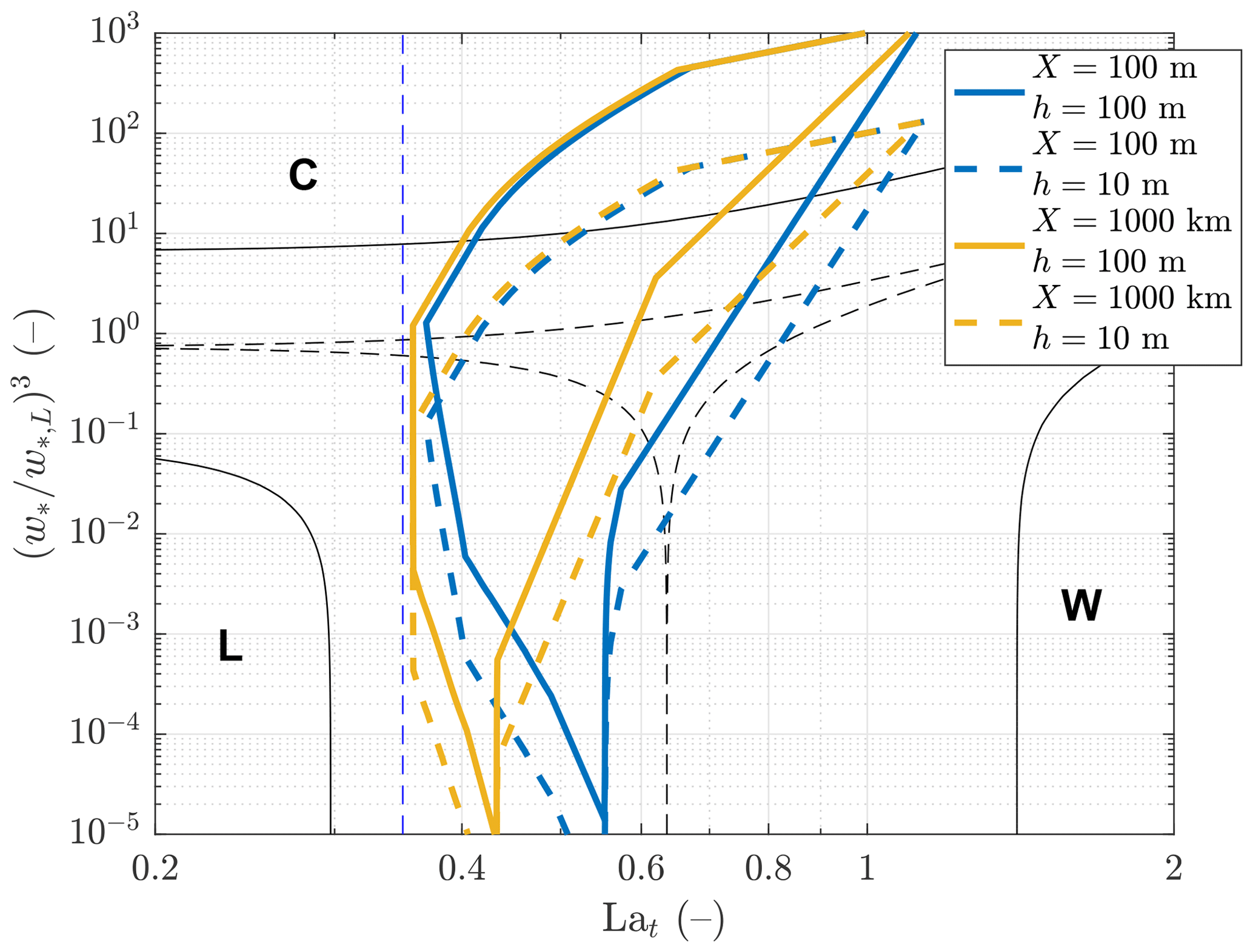
Figure 2 Regime diagram for OML mixing following Belcher et al. (2012). Continuous black lines delineate regions where at least 90 % of the total TKE is dissipated by only one of the three processes: Langmuir turbulence, wind shear, or convection (letters L, W, and C, respectively). Similarly, dashed black lines mark regions where TKE dissipation due to one process exceeds 50 % of the total dissipation. The thin dashed blue line is located at La_t=0.35, corresponding to fully developed waves. When the $(L{a}_t,w_{*}^{\mathrm{3}}/w_{*,\mathrm{L}}^{\mathrm{3}})$ pairs are computed for a range of wind, air temperature, and wave conditions described in the text, the corresponding points fall into a region marked with a color contour, the exact position and shape of which depends on the assumed value of the mixed layer depth h (continuous lines: h=100 m; dashed lines: h=10 m) and fetch X (blue: X=100 m; yellow: X=1000 km). See text for more details.

The OML dynamics under different mixing regimes has been analyzed numerically and theoretically in several studies (Chamecki et al., 2019). However, a great majority of those studies concentrate on non-convective situations, i.e., on combined shear- and wave-driven OMLs. Especially large-eddy simulations with models including relevant wave-phase-averaged effects associated with the Stokes drift velocity (the vortex force, the Coriolis–Stokes term, advection of water properties brought about by wave-induced Lagrangian motion, etc.) have provided valuable insights into the nature of Langmuir circulation and transport. Under highly idealized conditions, the average combined Ekman–Stokes flow can be computed analytically (McWilliams et al., 1997). In realistic, turbulent conditions, Langmuir “cells” rarely form regular, uniformly spaced, and steady patterns but rather have a transient nature and tend to deform and merge with each other forming Y junctions pointing in a downwind direction (Thorpe, 2004; Sullivan and McWillliams, 2010). Although several aspects of the unstable character of Langmuir circulation (or, rather, Langmuir turbulence) remain poorly understood, LES models successfully reproduce those features (McWilliams et al., 1997; Chamecki et al., 2019, and references therein). The low-order statistics of the OML flow and turbulence (mean profiles of velocity, velocity variance, TKE, TKE dissipation, etc.), as well as details of the 3D structure of the flow, depend on several factors, including stratification, entrainment from the pycnocline (Grant and Belcher, 2009), misalignment between the wind/wave direction (Van Roekel et al., 2012), the Ekman depth scale and thus the Coriolis parameter (Polton and Belcher, 2007), wave age and spectral characteristics (Harcourt and D'Asaro, 2008), and the transient evolution of wind/wave forcing (Sullivan et al., 2012). As already mentioned, OML mixing under vertically unstable, i.e., convective, conditions has been less intensively studied (Deardorff, 1972; Moeng and Sullivan, 1994). Notably, whereas until very recently LES studies were limited to idealized conditions and their results could rarely be validated with observations, LES methods are increasingly being applied to real ocean conditions with complex, spatially and temporarily varying forcing (e.g., Fan et al., 2020).

Not surprisingly, the 3D structure of OML circulation and turbulence has an essential influence on the transport and dispersion of particles in the upper ocean: oil droplets, gas bubbles, microplastics, sediment grains, phytoplankton, and ice crystals. Following Chamecki et al. (2019), those particles can be divided into passive tracers (following the motion of the surrounding water), floaters (always remaining at the surface), and sinking and buoyant particles (with densities higher and lower, respectively, than the density of the surrounding water). In the great majority of studies, any inertial effects that might accompany the motion of the particles are ignored so that the horizontal component of their velocity is u_p=u and the vertical component is $w_{\mathrm{p}}=w+w_{\mathrm{t}}$, where (u, w) is the water velocity and w_t is the terminal velocity of the particles. For the four particle types mentioned before, w_t=0, w_t→∞, w_t<0, and w_t>0, respectively. Combined with the three velocity scales introduced earlier, u_*, w_*, and $w_{*,\mathrm{L}}$, the value of w_t is crucial for the fate of the suspended material in the OML. Chor et al. (2018b), who analyzed the OML transport of positively buoyant particles under pure convection, introduced a floatability parameter defined as the ratio $w_{\mathrm{t}}/w_{*}$ and demonstrated that the preferential concentration of particles in the surface convergence zones occurs for sufficiently high values of that parameter – particles with very low floatability are pulled down with the downwelling currents and resurface again in surface divergence regions, being effectively distributed over the entire OML, whereas particles with high floatability resurface fast enough to stay trapped within the convergence zones. As w_t depends on particles' density, size, and shape, when multiple particle “classes” are present in the OML, smaller and/or denser ones tend to behave in the first manner and larger/lighter ones in the second manner, producing a de-mixing effect. Apart from this basic mechanism generating preferential particle concentration in OML, another effect, relevant for objects with high $w_{\mathrm{t}}/w_{*}$, leads to their accumulation in regions with high vorticity (Chor et al., 2018b).

Arguably, an analogous ratio of velocity scales can be defined for wave-forced OMLs, $w_{\mathrm{t}}/w_{*,\mathrm{L}}$, with a similar influence on particle behavior. This idea was expanded upon by Chor et al. (2018a), who proposed a combined velocity scale including all three TKE dissipation mechanisms. In turn, Yang et al. (2014) in their study on oil dispersion by Langmuir circulation use the ratio u_S∕w_t, which they call the drift-to-buoyancy parameter; i.e., they treat u_S as a simple proxy of downwelling velocity in the OML circulation. Based on the results of LES simulations, Yang et al. (2014) show that the forms of the surface oil slicks can be divided into three regimes, fingered, blurred, and diluted, which are dependent on the value of u_S∕w_t. In the fingered regime, for $u_{\mathrm{S}}/w_{\mathrm{t}}<\mathrm{10}$, oil droplets accumulate in windrows and are transported mostly in the wind/wave direction. In the diluted regime, for $u_{\mathrm{S}}/w_{\mathrm{t}}>\mathrm{25}$, the droplets are distributed over the entire OML so that no clear structure of oil patches is visible and the net oil transport is directed at an angle to the wind direction (see also Yang et al., 2015). Thus, the floatability of suspended particles influences not only the vertical profiles of their mean concentration (as studied, e.g., by Kukulka et al., 2012; Yang et al., 2014; Kukulka and Brunner, 2015; Chor et al., 2018a) but also their horizontal transport and diffusion (Yang et al., 2014, 2015).

Finally, it is worth stressing that in the majority of studies on material transport in the OML, including those cited above, an assumption is made that the volume concentration of suspended particles is sufficiently low so that the OML dynamics is not affected by their presence. The number of studies which explicitly concentrate on the influence of the transported material on OML behavior is rather limited. An example is the paper by Botte and Mansutti (2012) who used an LES model coupled with an ecosystem model to show that the influence of surfactants produced by phytoplankton on surface tension leads to the formation of regions of high surface shear stress, to higher vertical velocities in the water column, and to deeper mixing.

2.2 Mixing regimes and frazil transport in polynyas

As mentioned in the Introduction, most of the research on OML dynamics and material transport took place independently of research on frazil and grease ice formation – it is enough to say that, in the extensive review by Chamecki et al. (2019), cited earlier, the word “ice” is never used. Therefore, before proceeding to the details of the model and its setup, it is useful to take one more look at the issues referred to in the previous section, this time explicitly in the context of sea ice and conditions typical for its formation with particular stress on polynyas, which are of interest in this work.

The three velocity scales characterizing OML TKE dissipation, u_*, $w_{*,\mathrm{L}}$, and w_*, can be computed for a range of atmospheric and wave conditions that are likely to be found over coastal polynyas. Using the model of air–ocean heat and momentum exchange described in Sect. 3.2 and in Sect. S1 in the Supplement, u_* and w_* can be computed for a given combination of wind speed U_a and surface air temperature T_a with just one additional, poorly constrained parameter: the mixed layer depth h. As the waves in polynyas are likely locally generated (i.e., no swell is present), the wave characteristics necessary to compute $w_{*,\mathrm{L}}$ can be determined from wind speed and, again, one additional parameter: the fetch X. Details of the computation and definitions of the relevant variables can be found in Sect. S2. The $(La,w_{*}^{\mathrm{3}}/w_{*,\mathrm{L}}^{\mathrm{3}})$ pairs necessary to determine the mixing regime in the diagram of Belcher et al. (2012) have been computed for different combinations of U_a between 3 and 30 m s⁻¹, for T_a between −20 and −1 ^∘C, and for four possible combinations of two fetch values (100 m and 1000 km) and two mixed layer depths (10 and 100 m). The results are shown in Fig. 2. For the sake of legibility, no individual data points are plotted, just the boundary of regions surrounding them. As can be seen, in spite of large differences in X and h which correspond to very different conditions in terms of fetch (just offshore, at X=100 m, and very far from shore, where waves become X independent) and the vertical range of convection, the overall shape and position of the four regions remain relatively stable. All four regions are elongated in the $w_{*}^{\mathrm{3}}/w_{*,\mathrm{L}}^{\mathrm{3}}$ direction, with their lower/upper parts corresponding to situations with small/large $|T_{\mathrm{a}}-T_{\mathrm{w}}|$ differences and thus weak/strong convective forcing (T_w denotes surface water temperature, which is close to freezing point). A purely convection-dominated mixing regime (letter C in Fig. 2) requires not only T_a≪T_w but also very low wind speeds, i.e., conditions that are realistic only over short time periods, for example, immediately after the cessation of katabatic winds. Those conditions are conducive to ice formation in the form of nilas, with ice accumulation at the surface leading to a rapid decrease in ocean–atmosphere heat flux and eventually to the closing of the polynya.

At another extreme, when T_a≈T_w (lower part of the diagram in Fig. 2), the dissipation results from the combined effects of waves (Langmuir turbulence) and wind (vertical shear), which, without the influence of swell, are very closely related. It is also notable that as the Stokes drift amplitude u_S is proportional to a²∕T³, where a is the wave amplitude and T the wave period, the increase in a with increasing fetch and wind speed is partially compensated for by an accompanying increase in T (see equations in Sect. S2), which in effect reduces the range of values of La_t to between 0.35 and 0.55 (values of La<0.35 to the left of the thin dashed blue line in Fig. 2 correspond to swell).

In general, the effectiveness of convective dissipation and thus the contribution of convection to the total dissipation increases with increasing h. Observations show that under typical conditions during strong katabatic wind events, the mixed layer thickness often reaches a few hundreds of meters. Shallow mixed layers are not realistic under those conditions unless, of course, the total water depth is small, as in some coastal polynyas in the Arctic (e.g., Dethleff, 2005; Ito et al., 2019).

Overall, a mixed TKE dissipation regime should be typical for coastal polynyas with non-negligible contributions from all three mixing mechanisms but with the domination of convective mixing or Langmuir turbulence under very strong or relatively weak atmospheric cooling, respectively. Hence, all three mechanisms should be captured by any model intended to reproduce the OML behavior in those water bodies. Also important is that when sea ice formation takes place, it introduces an additional source of buoyancy related to salt rejection to the water column – an effect that has not hitherto been included in the discussion and that may additionally increase the relative role of convective processes.

As elaborated upon in the previous section, the fate of the forming frazil ice crystals in the turbulent OML depends largely on their rising velocity w_t in relation to the three OML velocity scales. For the conditions analyzed here, u_*, $w_{*,\mathrm{L}}$, and w_* reach 0.05, 0.1, and 0.02 m s⁻¹, respectively (Figs. S3 and S5). Anticipating the presentation of the results in Sect. 5, it is worth adding that instantaneous vertical velocity in downwelling plumes can be much higher and exceed 0.3–0.4 m s⁻¹. The terminal velocity of frazil crystals, computed from their radius and density (e.g., Holland and Feltham, 2005), is lower than 0.001 m s⁻¹ for crystals smaller than 0.1 mm and increases to ∼0.01 m s⁻¹ for crystals with radii greater than 1 mm. Thus, the floatability of frazil in the conditions of interest is low and less than 1 for most crystal size classes. Based on this elementary analysis alone, preferential concentration of frazil within the turbulent OML can be expected to occur only for the largest crystals.

3 Model description

The model code developed for this study is based on the Coastal and Regional Ocean COmmunity Model (CROCO), which is built upon the Regional Ocean Modeling System (ROMS; Shchepetkin and McWilliams, 2005). CROCO is an open-source hydrodynamic model developed for high-resolution, non-hydrostatic, and non-Boussinesq simulations of various flow types, especially at fine spatial and temporal scales. Examples of applications include coastal upwelling systems, frontal dynamics, internal waves, and 3D simulations of wave–current interactions in the coastal zone, as well as selected biogeochemical processes and sediment transport. In Sect. 3.1, we provide a short summary of the model features relevant for the setup used in this study; a detailed description of CROCO can be found in the documentation available through the model web page (http://www.croco-ocean.org, last access: 2 November 2020). In the subsequent Sects. 3.2 and 3.3, an in-depth description of new model features can be found, including details of the frazil module.

3.1 The CROCO model

The equations of CROCO are formulated in terms of the following wave-averaged variables: dynamic pressure $p_c=p+p_{\mathrm{w}}$, sea level ξ, density ρ, and velocity $({\mathbf{u}}_c,w_c)=(\mathbf{u},w)+({\mathbf{u}}_{\mathrm{S}},w_{\mathrm{S}})$, where p_w denotes the so-called Bernoulli head, which is related to the wave-averaged kinetic energy, and (u_S, w_S) denotes the Stokes velocity related to the wave motion. Thus, the total velocity (u_c, w_c) is a Lagrangian, wave-averaged velocity given as a sum of the Eulerian and Stokes components. In the notation used above, u_c, u, and u_S denote the horizontal components and w_c, w, and w_S the vertical components of the respective vectors. The governing equations are the momentum equations in the horizontal and vertical direction, the continuity equation, and the surface kinematic condition:

$$\begin{array}{}\text{(1)}& {\displaystyle }\begin{array}{rl}& {\displaystyle \frac{\partial \left(\mathit{\rho }\mathbf{u}\right)}{\partial t}}+\mathrm{\nabla }\cdot \left(\mathit{\rho }{\mathbf{u}}_c\mathbf{u}\right)+{\displaystyle \frac{\partial }{\partial z}}\left(\mathit{\rho }{w}_c\mathbf{u}\right)+f\mathit{\rho }{\mathbf{n}}_z\times {\mathbf{u}}_c=\\ & -\mathrm{\nabla }{p}_c+\mathit{\rho }{\mathbf{u}}_{\mathrm{S}}\mathrm{\nabla }\cdot \mathbf{u}+{\mathbf{F}}_h+{\mathbf{F}}_{\mathrm{w}},\end{array}\text{(2)}& {\displaystyle }\begin{array}{rl}& {\displaystyle \frac{\partial \left(\mathit{\rho }w\right)}{\partial t}}+\mathrm{\nabla }\cdot \left(\mathit{\rho }{\mathbf{u}}_{\mathbf{c}}w\right)+{\displaystyle \frac{\partial }{\partial z}}\left(\mathit{\rho }{w}_{c}w\right)=\\ & -{\displaystyle \frac{\partial p_c}{\partial z}}-\mathit{\rho }g+\mathit{\rho }{\mathbf{u}}_{\mathrm{S}}\cdot {\displaystyle \frac{\partial \mathbf{u}}{\partial z}}+F_v,\end{array}\text{(3)}& {\displaystyle \frac{\partial \mathit{\rho }}{\partial t}}+\mathrm{\nabla }\cdot \left(\mathit{\rho }\mathbf{u}\right)+{\displaystyle \frac{\partial }{\partial z}}\left(\mathit{\rho }{w}_c\right)=\mathrm{0},\text{(4)}& {\displaystyle \frac{\partial \mathit{\xi }}{\partial t}}+\mathbf{u}\cdot \mathrm{\nabla }\mathit{\xi }=w_{\mathit{\xi }},\end{array}$$

where ∇ is the horizontal gradient operator, f=2Ω_Zsin ϕ denotes the Coriolis parameter (with Ω_Z the angular velocity of the Earth and ϕ the latitude), g denotes acceleration due to gravity, n_z is a unit vector directed vertically upward, w_ξ is the vertical velocity at the surface, F_w denotes wave-related non-conservative forces (e.g., due to wave breaking), and (F_h, F_v) denotes non-conservative forces unrelated to waves (e.g., subgrid-scale turbulence). The treatment of the non-hydrostatic terms, including the relationship between pressure and density needed to close the system of Eqs. (1)–(3), is provided in the documentation of CROCO, cited above. The theoretical background underlying wave-related terms in Eqs. (1)–(3), together with derivation, boundary conditions, and discussion of the influence of individual terms on the mixed layer dynamics, can be found in McWilliams et al. (2004) and Uchiyama et al. (2010).

Equations (1)–(3) are supplemented by a transport equation for any scalar quantity α:

$$\begin{array}{}\text{(5)}& {\displaystyle \frac{\partial \left(\mathit{\rho }\mathit{\alpha }\right)}{\partial t}}+\mathrm{\nabla }\cdot \left(\mathit{\rho }{\mathbf{u}}_c\mathit{\alpha }\right)+{\displaystyle \frac{\partial }{\partial z}}\left(\mathit{\rho }{w}_c\mathit{\alpha }\right)=S_{\mathit{\alpha }}+S_{\mathit{\alpha },\mathrm{w}},\end{array}$$

where S_α and S_α, w denote the wave-unrelated and wave-related, non-conservative (forcing and diffusive) terms, respectively. The formulation of those terms depends on the type of “tracer” α. In particular, in the case of both temperature T and salinity S, the source terms include turbulent diffusion, as well as forcing from the atmosphere at the ocean surface (see below). In the case of frazil crystals, Eq. (5) is solved for the volume fraction of each frazil size class with source terms representing thermodynamic processes (not used in this study) and buoyancy, as described in detail in Sect. 3.3.

To solve the system of Eqs. (1)–(5), the equation of state is necessary, relating the density of water ρ_w to temperature and salinity, ${\mathit{\rho }}_{\mathrm{w}}={\mathit{\rho }}_{\mathrm{w}}(T,S)$. As in previous models of frazil processes (e.g., Holland and Feltham, 2005), a linearized equation of state is used:

$$\begin{array}{}\text{(6)}& {\mathit{\rho }}_{\mathrm{w}}={\mathit{\rho }}_{\mathrm{w},\mathrm{0}}[\mathrm{1}+{\mathit{\beta }}_{\mathrm{T}}(T-T_{\mathrm{0}})+{\mathit{\beta }}_{\mathrm{S}}(S-S_{\mathrm{0}}\left)\right],\end{array}$$

with ${\mathit{\rho }}_{\mathrm{w},\mathrm{0}}={\mathit{\rho }}_{\mathrm{w},\mathrm{0}}(T_{\mathrm{0}},S_{\mathrm{0}})=\mathrm{1028.15}$ kg m⁻³, $T_{\mathrm{0}}=-\mathrm{1}$ ^∘C, S₀=35 PSU, ${\mathit{\beta }}_{\mathrm{T}}=\mathrm{4}\times {\mathrm{10}}^{-\mathrm{5}}$ K⁻¹, and ${\mathit{\beta }}_{\mathrm{S}}=\mathrm{7.8}\times {\mathrm{10}}^{-\mathrm{4}}$ PSU⁻¹. In Eqs. (1)–(5), ρ=ρ_w if no ice is present or its influence on density is switched off; otherwise, ρ represents the density of the ice–water mixture, as described in Sect. 3.3.3.

In CROCO, the wave-related variables necessary to compute the wave-related terms in the governing equations can be obtained from a spectral wave model coupled with the hydrodynamic model. In this study, the model is run on a relatively small rectangular domain with periodic lateral boundaries, which implies conditions that are spatially uniform at the domain scale. Accordingly, it is assumed that the phase-averaged wave characteristics – significant wave height H_s, peak wave period T_p, etc. – are constant and depend exclusively on the assumed wind speed U_a and fetch X, i.e., that the wave field is stationary and fetch-limited. As described in Sect. S2, a simple empirical model is used to compute H_s(U_a, X) and T_p(U_a, X). From those wave characteristics, the Stokes drift and other wave-related variables are obtained, assuming monochromatic, non-breaking, deep-water waves. In particular, the amplitude of the Stokes drift at the sea surface, z=0, is given as follows:

$$\begin{array}{}\text{(7)}& u_{\mathrm{S}}={\mathit{\omega }}_{\mathrm{p}}{k}_{\mathrm{p}}{a}^{\mathrm{2}},\end{array}$$

where ω_p is the peak wave frequency, k_p is the corresponding wavenumber (in deep water, $k_{\mathrm{p}}={\mathit{\omega }}_{\mathrm{p}}^{\mathrm{2}}/g=\mathrm{4}{\mathit{\pi }}^{\mathrm{2}}g/T_{\mathrm{p}}^{\mathrm{2}}$), and $a=H_{\mathrm{s}}/\mathrm{2}$ is the wave amplitude.

The non-conservative forcing terms in Eqs. (1), (2) and (5) include turbulent viscosity and diffusion terms, F_t, h, F_t, v, and S_α, t, respectively. The Reynolds stresses and turbulent tracer fluxes required to compute those terms are as follows:

$$\begin{array}{}\text{(8)}& \stackrel{\mathrm{‾}}{{\mathbf{u}}^{\prime }{w}^{\prime }}=-K_M{\displaystyle \frac{\partial \stackrel{\mathrm{‾}}{\mathbf{u}}}{\partial z}}\mathrm{and}\stackrel{\mathrm{‾}}{{\mathit{\alpha }}^{\prime }{w}^{\prime }}=-K_{\mathit{\alpha }}{\displaystyle \frac{\partial \stackrel{\mathrm{‾}}{\mathit{\alpha }}}{\partial z}},\end{array}$$

where u^′, w^′, and α^′ are turbulent fluctuations around the slowly varying values denoted by overbars, and the eddy viscosity K_M and eddy diffusivity K_α have the following form:

$$\begin{array}{}\text{(9)}& K_M=c\sqrt{\mathrm{2}k}l{S}_M+\mathit{\nu }\mathrm{and}{K}_{\mathit{\alpha }}=c\sqrt{\mathrm{2}k}l{S}_{\mathit{\alpha }}+{\mathit{\nu }}_{\mathit{\alpha }},\end{array}$$

where ν and ν_α denote the molecular viscosity and diffusivity, respectively, S_M and S_α are stability functions describing the effects of stratification and shear, and the coefficient c depends on the form of S_M and S_α. The turbulent kinetic energy (TKE) per unit mass k and the length scale l are determined by the so-called generic length scale (GLS) method developed by Umlauf and Burchard (2003) and implemented in ROMS, and later in CROCO, by Warner et al. (2005). The advantage of GLS is that it provides a unified framework for a number of popular two-equation turbulence models, taking advantage of the similarities in their mathematical formulations. The GLS scheme solves the transport equation for k (common to all models) and the equation for a generic variable ψ, which is used to determine the length scale l from a relationship $\mathit{\psi }=(c_{\mathit{\mu }}^{\mathrm{0}}{)}^p{k}^m{l}^n$. The equations have the following forms:

$$\begin{array}{}\text{(10)}& {\displaystyle \frac{\partial k}{\partial t}}+\stackrel{\mathrm{‾}}{\mathbf{u}}\cdot \mathrm{\nabla }k={\displaystyle \frac{\partial }{\partial z}}\left({\displaystyle \frac{K_M}{{\mathit{\sigma }}_k}}{\displaystyle \frac{\partial k}{\partial z}}\right)+P+B-\mathit{\epsilon },\text{(11)}& {\displaystyle }\begin{array}{rl}{\displaystyle \frac{\partial \mathit{\psi }}{\partial t}}+\stackrel{\mathrm{‾}}{\mathbf{u}}\cdot \mathrm{\nabla }\mathit{\psi }& ={\displaystyle \frac{\partial }{\partial z}}\left({\displaystyle \frac{K_M}{{\mathit{\sigma }}_{\mathit{\psi }}}}{\displaystyle \frac{\partial \mathit{\psi }}{\partial z}}\right)\\ & +{\displaystyle \frac{\mathit{\psi }}{k}}(c_{\mathrm{1}}P+c_{\mathrm{3}}B-c_{\mathrm{2}}\mathit{\epsilon }{F}_{\mathrm{wall}}),\end{array}\end{array}$$

where the coefficients $c_{\mathit{\mu }}^{\mathrm{0}}$, c₁, c₂, c₃, σ_k, and σ_ψ and the wall proximity function F_wall, as well as the exponents p, m, and n, are model-dependent. The terms P and B denote production of k due to shear and buoyancy, respectively, and ε represents TKE dissipation (see Warner et al., 2005, for details and formulation of those terms,). Importantly, all those parameters can be adjusted to obtain the standard k–ε, k–ω, and k–kl models. In the simulations described in this paper, the k–ε GLS version was used (for which p=3.0, m=1.5, and $n=-\mathrm{1.0}$) with stability functions according to Canuto et al. (2001).

As the molecular diffusivity is much lower than the turbulent one in all situations considered here (O(10⁻⁷) m² s⁻¹ for heat, O(10⁻⁹) m² s⁻¹ for salt), all ν_α are assumed to be equal to zero. In the case of the viscosity ν, its value corresponds to the viscosity of water ν_w if no frazil is present or its influence is switched off; otherwise, it is computed as described in Sect. 3.3.3.

The horizontal mixing is computed with the Smagorinsky parametrization of lateral turbulent viscosity with a constant Prandtl number of 0.3.

Table 1 Setup of the CROCO model used in this study.

3.2 Forcing from the atmosphere

In the simplified model setting considered here, the state of the lower atmosphere is described by the following set of variables: wind speed vector at 10 m height U_a, air temperature and relative humidity, T_a and q_r, respectively, and surface atmospheric pressure p_a. The shortwave radiation flux and the precipitation rate are assumed to be equal to zero. The net heat flux at the ocean–atmosphere interface is computed as the sum of the turbulent latent and sensible heat flux, F_h and F_e, and the sum of the upward and downward long-wave radiation, F_rad. All flux components, as well as the wind stress τ_w and the surface salt flux due to evaporation H_e, are computed using modified bulk formulae from COAMPS (Coupled Ocean/Atmosphere Mesoscale Prediction System). They are described in Sect. S2. The major difference with respect to the analogous formulae available in the public version of CROCO is related to the computation of the transfer coefficients for heat, moisture, and momentum, which in CROCO are assumed constant. Here, in order to make them suitable for a wide range of conditions including very high wind speeds and, even more importantly, to allow for transfer coefficients varying in surface frazil volume fraction, they are variable. The general formulae are as follows:

$$\begin{array}{}\text{(12)}& C_d=C_{d,\mathrm{n}}{\mathit{\alpha }}_{\mathrm{s}},C_{\mathrm{h}}=C_{\mathrm{h},\mathrm{n}}{\mathit{\alpha }}_{\mathrm{s}},C_e=C_{e,\mathrm{n}}{\mathit{\alpha }}_{\mathrm{s}},\end{array}$$

where $C_{x,\mathrm{n}}=C_{x,\mathrm{n}}\left(U_{\mathrm{a}}\right)$ are neutral transfer coefficients (with x denoting d, h, or e for transfer of momentum, heat, and water, respectively), ${\mathit{\alpha }}_{\mathrm{s}}={\mathit{\alpha }}_{\mathrm{s}}(U_{\mathrm{a}},T_{\mathrm{w}}-T_{\mathrm{a}})$ is a stability parameter, and $U_{\mathrm{a}}=\left|{\mathbf{U}}_a\right|$.

3.3 Frazil processes

3.3.1 Definitions and assumptions

As in most similar models (e.g., Svensson and Omstedt, 1998; Holland and Feltham, 2005; Heorton et al., 2017), frazil is represented by $i=\mathrm{1},\mathrm{\dots },N_{\mathrm{f}}$ prescribed crystal size classes. It is assumed that the crystals are disk shaped so that their size in the ith class can be described by the radius r_i and thickness $h_i=a_{\mathrm{r},i}{r}_i$. In this study, following Holland and Feltham (2005), the aspect ratio a_r, i is assumed to be the same for each class, $a_{\mathrm{r}}=\mathrm{1}/\mathrm{50}$ (see Table 1). Similarly, a constant ice density is assumed, ρ_i=920 kg m⁻³. The amount of frazil from each size class in a given volume of sea water is described by ice volume fraction c_i ($\mathrm{0}\le c_i\le \mathrm{1}$). The total frazil volume fraction is $c={\sum }_{i=\mathrm{1}}^{N_{\mathrm{f}}}{c}_i$.

As mentioned in the Introduction, the thermodynamic model of frazil has been switched off in all simulations described in this paper. Consequently, the total domain-integrated mass of ice within each size class remains constant and is equal to its initial value (see further Sect. 4). The OML-averaged volume fraction of the ith class, ${\stackrel{\mathrm{̃}}{c}}_i$, is defined as ${\stackrel{\mathrm{̃}}{c}}_i=h^{-\mathrm{1}}{\int }_{z=-h}^{\mathrm{0}}{c}_{i}dz$.

3.3.2 Frazil transport

The transport of frazil crystals within the OML, as for every scalar quantity, is described in Eq. (5). Zero-flux boundary conditions are used at the surface and at the bottom of the model domain. In the full model version including ice thermodynamics, the source terms in Eq. (5) include those related to freezing or melting, secondary nucleation, etc. With those processes switched off, the only source term is related to the positive buoyancy of crystals and their precipitation towards the water surface. For each frazil size class i,

$$\begin{array}{}\text{(13)}& S_i=-{\displaystyle \frac{\partial }{\partial z}}\left(w_{t,\mathrm{i}}{c}_i\right),\end{array}$$

where w_t, i denotes the vertical velocity of ice relative to the surrounding water. In the uppermost layer of the model, $w_{t,\mathrm{i}}(z=\mathrm{0})=\mathrm{0}$. Elsewhere in the water column, disregarding inertial effects, w_t, i can be approximated with the terminal velocity of crystals which is computed from the balance between the gravity and buoyancy force:

$$\begin{array}{}\text{(14)}& \mathit{\pi }{a}_{\mathrm{r},i}{r}_i^{\mathrm{3}}({\mathit{\rho }}_{\mathrm{w}}-{\mathit{\rho }}_{\mathrm{i}})g={\displaystyle \frac{\mathrm{1}}{\mathrm{2}}}{C}_{\mathrm{D}}{\mathit{\rho }}_{\mathrm{w}}\mathit{\pi }{r}_i^{\mathrm{2}}{w}_{t,\mathrm{i}}^{\mathrm{2}},\end{array}$$

so that

$$\begin{array}{}\text{(15)}& \mathrm{2}{a}_{\mathrm{r},i}{\displaystyle \frac{{\mathit{\rho }}_{\mathrm{w}}-{\mathit{\rho }}_{\mathrm{i}}}{{\mathit{\rho }}_{\mathrm{w}}}}g={\displaystyle \frac{C_{\mathrm{D},i}{w}_{t,\mathrm{i}}^{\mathrm{2}}}{r_i}}.\end{array}$$

The widely used Schiller–Naumann model (Kolev, 2011) is used to calculate the drag coefficient C_D, i:

$$\begin{array}{}\text{(16)}& C_{\mathrm{D},i}=\left\{\begin{array}{ll}\frac{\mathrm{24}}{R{e}_i}\left(\mathrm{1}+\mathrm{0.15}R{e_i}^{\mathrm{0.687}}\right)& R{e}_i<\mathrm{1000}\\ \mathrm{0.44}& R{e}_i\ge \mathrm{1000}\end{array}\right.,\end{array}$$

where the relative (or particle) Reynolds number Re_i is calculated as follows:

$$\begin{array}{}\text{(17)}& R{e}_i={\displaystyle \frac{\mathrm{2}{r}_i{w}_{t,\mathrm{i}}}{{\mathit{\nu }}_{\mathrm{w}}}}.\end{array}$$

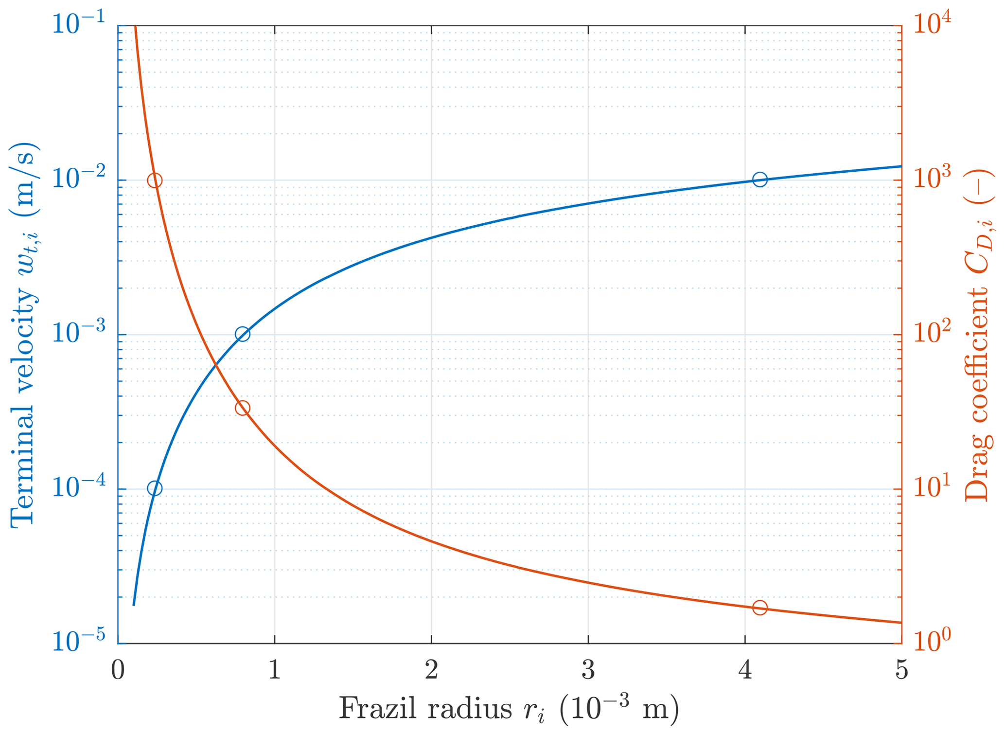
For realistic values of r_i, Re_i≪1000 so that the first expression in Eq. (16) is relevant. The values of w_t, i and C_D, i obtained from Eqs. (15)–(17) for a range of frazil radii r_i is shown in Fig. 3. Notably, although simple, this model is in broad agreement with observed relationships between frazil crystal size and rise velocity, as well as with the existing theoretical models (see McFarlane et al., 2014, and references therein). When necessary, Eqs. (15)–(17) can be easily replaced with more complex ones, e.g., with models taking into account crystal orientation (in the present study, concentrating on turbulent conditions, the assumption of random orientation seems justified).

Figure 3 Terminal velocity w_t, i (left axis) and drag coefficient C_D, i (right axis) computed from formulae (15)–(17) for frazil radii r_i between 0.1 and 5.0 mm. Circles mark the values used in the simulations analyzed in this study (see Table 1).

3.3.3 Frazil influence on hydrodynamics

In the simulations in Sect. 5, the presence of frazil is allowed to modify the OML dynamics by influencing four variables: the net density ρ, the net neutral transfer coefficients at the ocean–atmosphere interface ${\widehat{C}}_{x,n}$, the effective viscosity ν, and the drag force F_D exerted by the rising frazil crystals on the surrounding water. The density of the water–ice mixture is as follows:

$$\begin{array}{}\text{(18)}& \mathit{\rho }=(\mathrm{1}-c){\mathit{\rho }}_{\mathrm{w}}+c{\mathit{\rho }}_{\mathrm{i}}.\end{array}$$

For the transfer coefficients, a linear relationship is assumed for frazil volume fractions between c=0 and c=c_lim and a constant value $C_{x,n,\lim }$ for c>c_lim:

$$\begin{array}{}\text{(19)}& {\widehat{C}}_{x,n}=max\mathit{\{}{C}_{x,n}+(C_{x,n,\lim }-C_{x,n})c/c_{\lim },C_{x,n,\lim }\mathit{\}},\end{array}$$

where C_x, n is computed from formulae (12). We assume $C_{x,\lim }<C_x$, i.e., in agreement with observations, the presence of frazil and grease ice leads to a decrease in the ocean–atmosphere heat and momentum exchange (contrary to other sea ice types, for which, in the case of momentum transfer, the effect is opposite). The roughness length of grease ice equals $\mathrm{2.7}\times {\mathrm{10}}^{-\mathrm{6}}$ m (compared to, e.g., $\mathrm{1.0}\times {\mathrm{10}}^{-\mathrm{3}}$ m for pancake ice and 1.3–$\mathrm{2.4}\times {\mathrm{10}}^{-\mathrm{3}}$ m for first-year ice), and its neutral drag coefficient is as low as $\mathrm{0.7}\times {\mathrm{10}}^{-\mathrm{3}}$ (Guest and Davidson, 1991).

Several models have been used in the literature to compute the effective viscosity ν of the water–ice mixture. Here, following Matsumura and Ohshima (2015), a simple expression is used:

$$\begin{array}{}\text{(20)}& \begin{array}{rl}& \mathit{\nu }=\\ & {\mathit{\nu }}_{\mathrm{w}}\left[\mathrm{1}+\mathrm{2.5}{c}_{\mathrm{rel}}+\mathrm{10.05}{c}_{\mathrm{rel}}^{\mathrm{2}}+\mathrm{2.73}\times {\mathrm{10}}^{-\mathrm{3}}\exp \left(\mathrm{16.6}{c}_{\mathrm{rel}}\right)\right],\end{array}\end{array}$$

in which $c_{\mathrm{rel}}=min\mathit{\{}c/c_{\max },\mathrm{1.0}\mathit{\}}$ and c_max is the maximum ice volume fraction corresponding to typical values for grease ice. For c_rel=0, ν=ν_w; for c_rel=1, $\mathit{\nu }=\mathrm{4}\times {\mathrm{10}}^{\mathrm{4}}{\mathit{\nu }}_{\mathrm{w}}$, which is in agreement with observations (e.g., Martin and Kauffman, 1981; Newyear and Martin, 1997). More advanced models for ν have been proposed (e.g., De Carolis et al., 2005), but their range of applicability is often limited to a narrow range of conditions (e.g., very low ice concentration). For the present idealized modeling study, formula (20) is sufficient to capture the leading-order effects related to the ν(c) variability.

Following Covello et al. (2016), the net liquid–solid drag force for a single dispersed phase can be computed from the following:

$$\begin{array}{}\text{(21)}& F_{\mathrm{D},i}=\left\{\begin{array}{ll}-\frac{\mathrm{3}{\mathit{\rho }}_{\mathrm{w}}{C}_{\mathrm{D},i}{w}_{t,\mathrm{i}}^{\mathrm{2}}}{\mathrm{8}{r}_i}\frac{c_i}{(\mathrm{1}-c_i{)}^{\mathrm{1.65}}}& c_i\le \mathrm{0.2}\\ -\frac{\mathrm{75}{\mathit{\rho }}_{\mathrm{w}}{\mathit{\nu }}_{\mathrm{w}}{w}_{t,\mathrm{i}}}{\mathrm{2}{r}_i^{\mathrm{2}}}\frac{c_i}{\mathrm{1}-c_i}-\frac{\mathrm{7}{\mathit{\rho }}_{\mathrm{w}}{w}_{t,\mathrm{i}}^{\mathrm{2}}}{\mathrm{16}{r}_i}{c}_i& c_i>\mathrm{0.2}\end{array}\right..\end{array}$$

Importantly, this formulation is consistent with formulae (15)–(17) used to compute the terminal velocity w_t, i. Moreover, for c_i≤0.2 – which is true for the great majority of cases analyzed in this study – it follows from Eq. (15) that the term ${\mathit{\rho }}_{\mathrm{w}}{C}_{\mathrm{D},i}{w}_{t,\mathrm{i}}^{\mathrm{2}}/r_i$ is constant and equal to 2a_r(ρ_w−ρ_i)g (black curve in Fig. 4). Therefore, the net F_D is computed from the total ice volume fraction:

$$\begin{array}{}\text{(22)}& F_{\mathrm{D}}=\left\{\begin{array}{ll}-\frac{\mathrm{3}{a}_{\mathrm{r}}({\mathit{\rho }}_{\mathrm{w}}-{\mathit{\rho }}_{\mathrm{i}})g}{\mathrm{4}}\frac{c}{(\mathrm{1}-c{)}^{\mathrm{1.65}}}& c\le \mathrm{0.2}\\ -\frac{\mathrm{75}{\mathit{\rho }}_{\mathrm{w}}{\mathit{\nu }}_{\mathrm{w}}{\stackrel{\mathrm{̃}}{w}}_t}{\mathrm{2}{\stackrel{\mathrm{̃}}{r}}^{\mathrm{2}}}\frac{c}{\mathrm{1}-c}-\frac{\mathrm{7}{\mathit{\rho }}_{\mathrm{w}}{\stackrel{\mathrm{̃}}{w}}_t^{\mathrm{2}}}{\mathrm{16}\stackrel{\mathrm{̃}}{r}}c& c>\mathrm{0.2}\end{array}\right.,\end{array}$$

where ${\stackrel{\mathrm{̃}}{w}}_t$ and $\stackrel{\mathrm{̃}}{r}$ denote volume-fraction-weighted average rising speed and radius, respectively.

Figure 4 Drag force F_D, i induced by the vertical motion of frazil crystals in function of frazil volume fraction c_i. For c_i<0.2, F_D, i is independent of frazil size (black curve). For c_i>0.2, three curves are shown corresponding to the three values of frazil radius r_i used in the simulations discussed in this paper (see also circle symbols in Fig. 3).

Crucially, although the modified version of CROCO includes the frazil-induced effects described in Eqs. (18)–(22), the general form of the governing equations, described in Sect. 3.1, remained unaffected. Thus, formally the model is only valid for total ice volume fraction c≪1, not for a mixture of water and ice with any c≤1, and care should be taken that the condition of small c is not violated during model applications.

Table 2 Model forcing computed for different combinations of U_a and T_a with formulae described in Sect. S1.

3.4 Model testing

No validation against observational data has been performed in this study. In order to test the suitability of the configuration of CROCO described above to the conditions of interest, the model has been set up to reproduce the test case analyzed by McWilliams et al. (1997) and later by Yang et al. (2015) with reference to observational data by D'Asaro (2001). The test case is in several aspects very similar to the setup considered here. The results are presented and discussed in Sect. S3. Additionally, a qualitative comparison of our results has been made with the results of Chen et al. (2016) and Chor et al. (2018b). We return to the issue of the validation of the modeling results in the discussion.

4 Model configuration

In this work, an idealized model setup is used. The model domain is cuboid and placed at the latitude ϕ=75^∘ N with periodic lateral boundaries in both horizontal directions, covering the upper 150 m of the ocean within an area of 1200 m × 1200 m. The horizontal resolution Δx equals 3 m, and there are 60 non-uniformly distributed layers so that the vertical resolution Δz varies from 0.5 m at the surface to 9.2 m at the lower boundary. A summary of all model parameters is given in Table 1.

The model is initialized with spatially uniform salinity and temperature profiles with the initial mixed layer depth h=100 m and

$$\begin{array}{}\text{(23)}& {\displaystyle }T\left(z\right)=\mathit{\delta }T+\left\{\begin{array}{ll}-\mathrm{1.5}& z\ge -h\\ -\mathrm{0.5}& z<-h\end{array}\right.,\text{(24)}& {\displaystyle }S\left(z\right)=\mathit{\delta }S+\left\{\begin{array}{ll}\mathrm{34.0}& z\ge -h\\ \mathrm{35.0}& z<-h\end{array}\right.,\end{array}$$

where $\mathit{\delta }S(x,y,z)$ and $\mathit{\delta }T(x,y,z)$ are random numbers drawn from a uniform distribution over an interval $(-\mathrm{0.005},\mathrm{0.005})$ PSU and $(-\mathrm{0.025},\mathrm{0.025})$ ^∘C, respectively, added to the profiles in order to introduce an initial disturbance to the otherwise perfectly uniform conditions. The water velocity is initialized with a horizontally uniform, steady-state Stokes–Ekman solution (McWilliams et al., 1997) in order to reduce the model spin up time. A free-slip boundary condition is applied at the lower boundary.

In simulations with frazil thermodynamics, it is important that the number of frazil size classes N_f is sufficiently large so that the crystal size distribution and interactions between different classes can be correctly captured. In this study with frazil thermodynamics switched off, N_f is set to three, and the radii of crystals are selected so that their terminal velocities equal 10⁻⁴ m s⁻¹ (for r₁=0.24 mm), 10⁻³ m s⁻¹ (for r₂=0.80 mm), and 10⁻² m s⁻¹ (for r₃=4.10 mm); see circle symbols in Fig. 3. For all i, the same OML-average volume fraction is set, ${\stackrel{\mathrm{̃}}{c}}_i=\mathrm{0.00168}$, which corresponds to a layer of ice with a thickness of 0.168 m for each class and a total ice thickness of 0.5 m. At time t=0, frazil is uniformly distributed over the upper 0.8 h of the model domain (tests have shown that the initial spatial distribution of frazil does not influence the final results).

The simulations were performed for different combinations of the following variable parameters: the air temperature T_a and wind speed U_a. The wind/wave direction is along the x axis. The corresponding wave forcing, net heat flux from the atmosphere, wind stress, and the velocity scales u_*, w_*, and $w_{*,\mathrm{L}}$ are listed in Table 2. The wind fetch X was set to 100 km. Some tests with very small X equal to 1000 m have been performed but are not discussed here as their results do not alter the conclusions from model runs with large X (although, obviously, there are quantitative differences in the modeled velocity profiles and other characteristics). Test model runs with h<100 m have been performed as well, but very fast deepening of the OML was observed due to strong mixing so that the final results were close to those obtained with h=100 m.

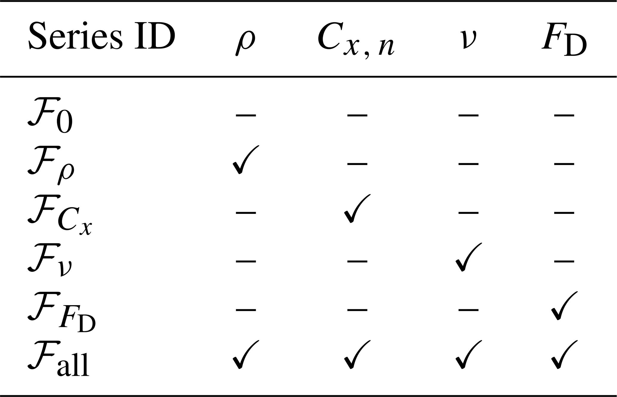
For each combination of T_a and U_a, six series of simulations were run (Table 3), differing in terms of coupling between the frazil and hydrodynamic parts of the model: from ℱ₀ in which the hydrodynamics is unaffected by the presence of frazil (and which is treated as a reference case for the remaining simulations) to ℱ_all in which all four interaction mechanisms described in Sect. 3.3.3 are activated.

Table 3 Main series of simulations discussed in the study with information on activated (✓) and deactivated (–) frazil interaction mechanisms.

The model equations are solved with a time step Δt=0.25 s so that the Courant number is much less than 1. Each simulation is 18 h long. The last 12 h of each run (corresponding approximately to one inertial period) are used in the result analysis. As shown in the examples in Sect. S4, the spin-up time of 6 h is sufficient for a quasi-stationary state to develop with stable domain-averaged vertical profiles of frazil volume fractions (and other important OML characteristics, not shown).

In the following section, time-averaged and horizontally averaged variables are denoted with brackets, 〈⋅〉, and with a bar, respectively. Anomalies from the averaged values are denoted with primes.

5 Modeling results

5.1 Series ℱ₀: no frazil→hydrodynamic coupling

The results of simulations from series ℱ₀, in which the hydrodynamic part of the model is unaffected by the presence of frazil, can be used to analyze the general behavior of the model in the range of forcing conditions considered, as well as to describe the redistribution of frazil particles of different sizes by the OML currents. Series ℱ₀ serves also as a point of reference for subsequent model runs.

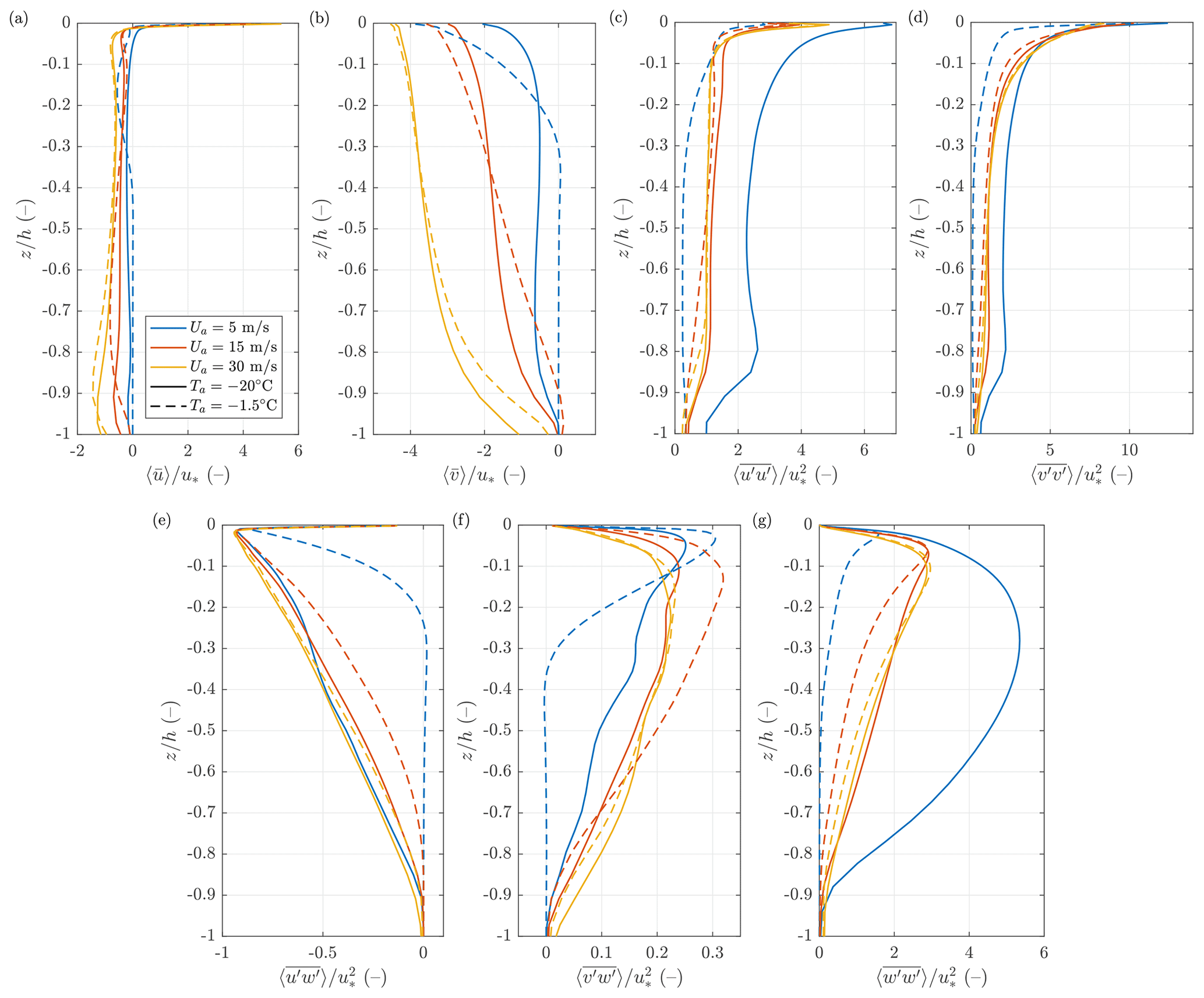
Figure 5 Vertical profiles of the mean velocity (a, b), momentum flux (e, f), and velocity variance (c, d, g) for different combinations of U_a (colors) and T_a (line styles). Results of simulations without frazil coupling (series ℱ₀). All values are normalized with the respective friction velocity u_*.

Figure 5 shows the vertical profiles of the time- and domain-averaged current velocities $\langle \overline{u}\rangle \left(z\right)$ and $\langle \overline{v}\rangle \left(z\right)$, momentum flux $\langle \stackrel{\mathrm{‾}}{u^{\prime }{w}^{\prime }}\rangle$ and $\langle \stackrel{\mathrm{‾}}{v^{\prime }{w}^{\prime }}\rangle$, and velocity variance $\langle \stackrel{\mathrm{‾}}{u^{\prime }{u}^{\prime }}\rangle$, $\langle \stackrel{\mathrm{‾}}{v^{\prime }{v}^{\prime }}\rangle$, and $\langle \stackrel{\mathrm{‾}}{w^{\prime }{w}^{\prime }}\rangle$ for different combinations of U_a and T_a. The overall vertical structure of the mean flow is similar to that known from earlier studies and predicted by theory: the x (along-wind) component of velocity exhibits positive values in a thin layer at the surface and negative elsewhere, which compensates for the positive Stokes drift. The y (across-wind) component is negative (in the Northern Hemisphere) and decreases with depth, faster as the wind speed lowers. Notably, when the air temperature is low and convection is present (continuous lines in Fig. 5), the velocity profiles are close to vertical over most of the OML with pronounced vertical velocity gradients only within relatively thin layers at the top and bottom of the OML. In the convection-dominated case with $T_{\mathrm{a}}=-\mathrm{20}$ ^∘C and U_a=5 m s⁻¹, the variance of the horizontal and, especially, the vertical velocity components is large over the entire OML due to the dominating influence of convective cells on the 3D flow structure. With weak forcing ($T_{\mathrm{a}}=-\mathrm{1.5}$ ^∘C and U_a=5 m s⁻¹), the flow is mostly limited to the upper parts of the OML. In the remaining cases (yellow and red curves in Fig. 5), the vertical profiles of momentum flux and velocity variance tend to be similar with very uniform, nearly linear variability far from the top and bottom of the OML.

The average vertical distribution of frazil (Fig. 6a, d, g) is a result of competition between mixing tending to homogenize frazil volume fractions over the entire OML and ice buoyancy tending to concentrate frazil at the sea surface. Not surprisingly, the shape of the equilibrium profiles of $\langle {\overline{c}}_i\rangle \left(z\right)$ changes with the crystal size and thus floatability. The smallest crystals (Fig. 6a) exhibit nearly uniform profiles under all analyzed conditions except for the lowest wind speed and high air temperature (dashed blue line). The largest crystals (Fig. 6g) tend to accumulate in the surface layer, and, especially when convection is weak, their mean concentration exhibits a clear vertical gradient. Under weak wind and weak convection, the area-averaged surface volume fraction $\langle {\overline{c}}_{\mathrm{3}}\rangle$ within the top-most model layer exceeds 10 times the OML average; combined with very high variance at the surface, this means that, locally, ice concentration reaches values greater than 0.2, corresponding to grease ice (dashed blue lines in Fig. 6g, h). For the smallest crystals, concentration variance is very small with maxima in the lowest parts of the OML where the plumes of frazil-laden OML water interact with the water from the pycnocline (as can be seen in Fig. 5a and b, in simulations with the strongest wind, the horizontal flow reaches to the bottom of the OML, which, combined with strong vertical currents in downwelling regions, leads to mixing with water underlying the OML). In the case of the largest crystals which only occasionally reach the bottom of the OML, there is no corresponding deep maximum of $\langle \stackrel{\mathrm{‾}}{c_{\mathrm{3}}^{\prime }{c}_{\mathrm{3}}^{\prime }}\rangle$ (Fig. 6h).

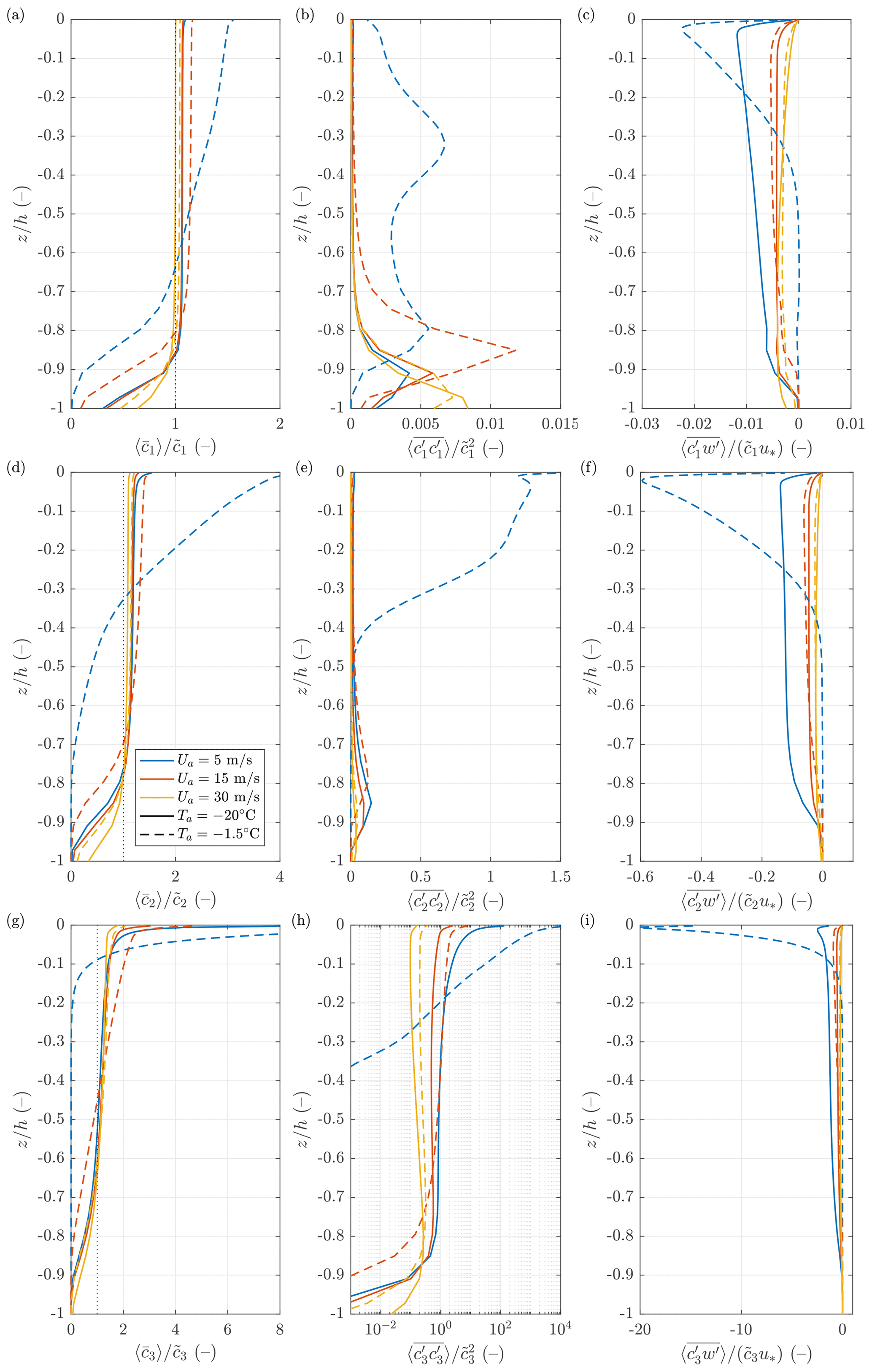
Figure 6 Vertical profiles of the mean (a, d, g), variance (b, e, h), and vertical flux (c, f, i) of the frazil volume fraction for size classes 1–3 for different combinations of U_a (colors) and T_a (line styles). Note the different x-axis ranges in the plots; in (h), the x axis is logarithmic.

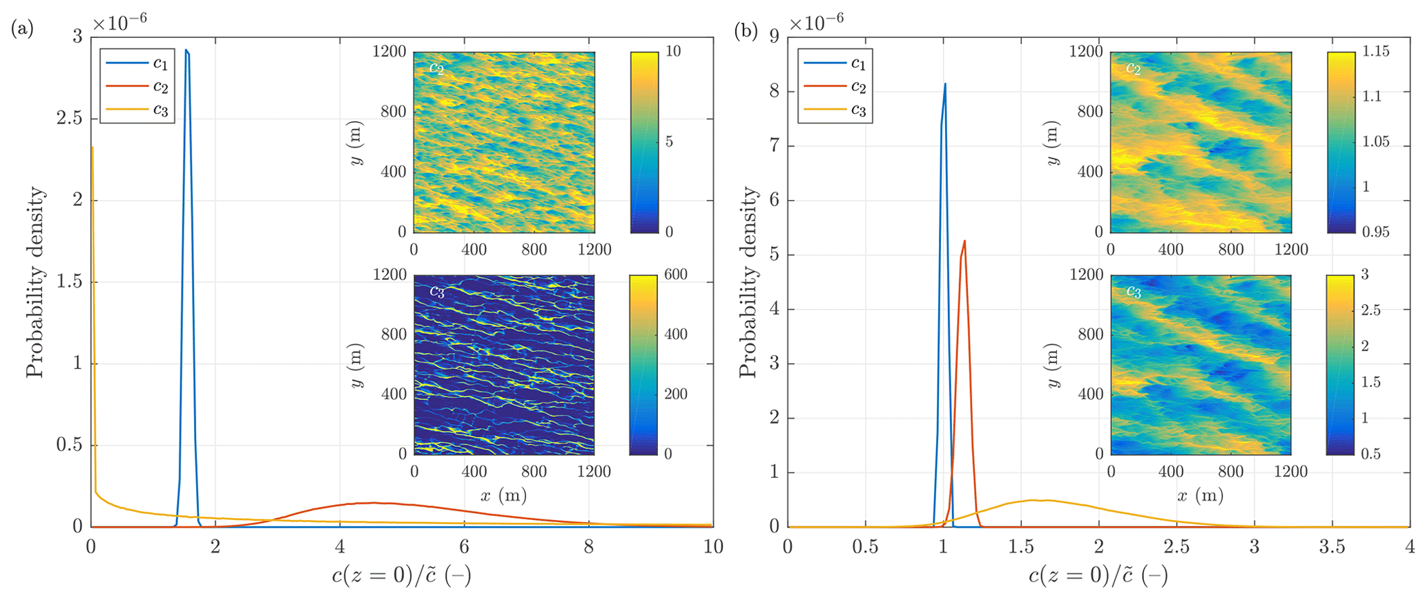
Figure 7 Distribution of frazil at the sea surface in simulations with (a) U_a=5 m s⁻¹ and $T_{\mathrm{a}}=-\mathrm{1.5}$ ^∘C and (b) U_a=30 m s⁻¹ and $T_{\mathrm{a}}=-\mathrm{20}$ ^∘C. The main plots show probability distributions of frazil volume fraction (normalized with $\stackrel{\mathrm{̃}}{c}$) at the surface (z=0) for all three size classes. All curves shown integrate to the value of 1. The insets show snapshots of $c_i/{\stackrel{\mathrm{̃}}{c}}_i$ for i=2 (top) and i=3 (bottom).

The strong near-surface maxima of both $\langle {\overline{c}}_{\mathrm{3}}\rangle$ and $\langle \stackrel{\mathrm{‾}}{c_{\mathrm{3}}^{\prime }{c}_{\mathrm{3}}^{\prime }}\rangle$ are manifestations of clustering of large crystals within the upper 1–2 m of the water column, as illustrated for two select cases in Fig. 7. Under calm conditions, this process is so effective that the volume fraction c₃ over a substantial part of the sea surface is close to zero (yellow curve and lower inset in Fig. 7a). Under the most turbulent conditions considered here, even the largest frazil fraction undergoes substantial mixing, but the preferential concentration still takes place and leads to wide probability distributions of c₃ at the surface (Fig. 7b).

Figure 8 Snapshots of the frazil volume fraction $c_{\mathrm{3}}/{\stackrel{\mathrm{̃}}{c}}_{\mathrm{3}}$ (a, b) and horizontal divergence D (c, d; in s⁻¹) at the surface, z=0, from simulations with U_a=15 m s⁻¹ and $T_{\mathrm{a}}=-\mathrm{1.5}$ ^∘C. Maps in (b, d) are zoomed fragments of those in (a, c). In (b), arrows show the velocity anomaly $(u-\langle u\rangle ,v-\langle v\rangle )$. The inset in (a) shows the vectors of mean velocity 〈u〉 and Stokes velocity u_S at the surface.

As can be seen in Fig. 6, the values of $\langle \stackrel{\mathrm{‾}}{c_i^{\prime }{w}^{\prime }}\rangle$ are negative in all cases analyzed; i.e., positive anomalies of frazil concentration occur in regions with negative vertical velocities, which in turn are located under the surface convergence zones. The zoomed panels in Fig. 8 clearly show that relationship, as well as the fact that the individual convergence zones tend to be narrow, elongated, and oriented approximately in the wind/wave propagation direction. The model reproduces also the characteristic pattern of Y-shaped junctions formed by those zones, known from observations and earlier modeling studies on Langmuir turbulence (Thorpe, 2004). Remarkably, the maps of ice concentration at the domain scale reveal two overlapping patterns: one related to the locally elevated values of c in individual convergence zones and the other in the form of wider, long streaks oriented obliquely to the wind/wave direction with a typical spacing of hundreds of meters. Accordingly, although it might seem surprising, the correlation between c and horizontal divergence D at the surface is low (in the example illustrated in Fig. 8 it equals −0.37). It increases significantly when the local anomaly of c, computed over an area l² surrounding a given location, is used instead of c itself (e.g., −0.71 for l=18 m in the example in Fig. 8). The larger-scale streaks of frazil, although clearly discernible in all modeling results with wind greater than or equal to 15 m s⁻¹, have irregular shapes and spacing, and their form constantly evolves in time, which, qualitatively, agrees with observations (see, e.g., photographs and satellite images in Eicken and Lange, 1989; Ciappa and Pietranera, 2013; Hollands and Dierking, 2016; Thompson et al., 2020). In particular, it can be seen in Fig. 7 of Ciappa and Pietranera (2013) that each streak has its own substructure and consists of several smaller patches and that the wave direction is not aligned with streak orientation (see also Hollands and Dierking, 2016). The observed separation between frazil streaks of 300–500 m reported in the cited studies is comparable with that obtained in our simulations. The example in Fig. 8, as well as other simulated cases (not shown), suggests that the overall orientation of the streaks corresponds approximately to the net direction of the surface Stokes drift u_S and the domain-mean surface current u (see inset in Fig. 8a).

As the lengths of the streaks are comparable with the size of the model domain, which might influence their formation and properties, a test simulation was performed for the case discussed above (U_a=15 m s⁻¹, $T_{\mathrm{a}}=-\mathrm{1.5}$ ^∘C) with all model settings unchanged but over a larger domain with dimensions 2L_x×2L_y, i.e., 2400 m × 2400 m. The results are presented in Sect. S5. As can be seen, the overall pattern of the surface ice concentration, as well as the bulk characteristics of the OML circulation and frazil transport, is insensitive to the domain size (the only noteworthy differences occur for $\langle \stackrel{\mathrm{‾}}{c_i^{\prime }{w}^{\prime }}\rangle$, but they never exceed 4 %–5 %). Therefore, although some influence of the limited domain size and periodic boundaries on the streak geometry cannot be ruled out, the general observations made above should remain valid.

Finally, it is also worth stressing that the vertical distribution of frazil and the basic properties of streaks described above are not sensitive to the latitude at which the model domain is located (see Sect. S6 for example results).

5.2 Modification of OML circulation by frazil-related processes

As shown in Table 3, the reference simulations from series ℱ₀ were followed by five series in which just one or all four frazil-related processes were activated. Overall, the effects due to the net viscosity and transfer coefficients at the sea surface (series ℱ_ν and ℱ_C, x) are minor compared to those related to net drag force and, especially, the net density (series ${\mathcal{F}}_{F_{\mathrm{D}}}$ and ℱ_ρ). This is particularly true as far as the mean characteristics of the OML circulation and frazil distribution are concerned. Consequently, the differences between the results of ℱ₀ and ℱ_all – which are substantial for most combinations of T_a and U_a – are dominated by the effects related to the lowered density of the ice–water mixture and, to a lesser extent, to the drag force induced by the rising ice crystals on the surrounding water. Figures 9 and 10 show an example for U_a=30 m s⁻¹ and $T_{\mathrm{a}}=-\mathrm{20}$ ^∘C for all six series. The conclusions from this case are valid for the other forcing combinations as well.

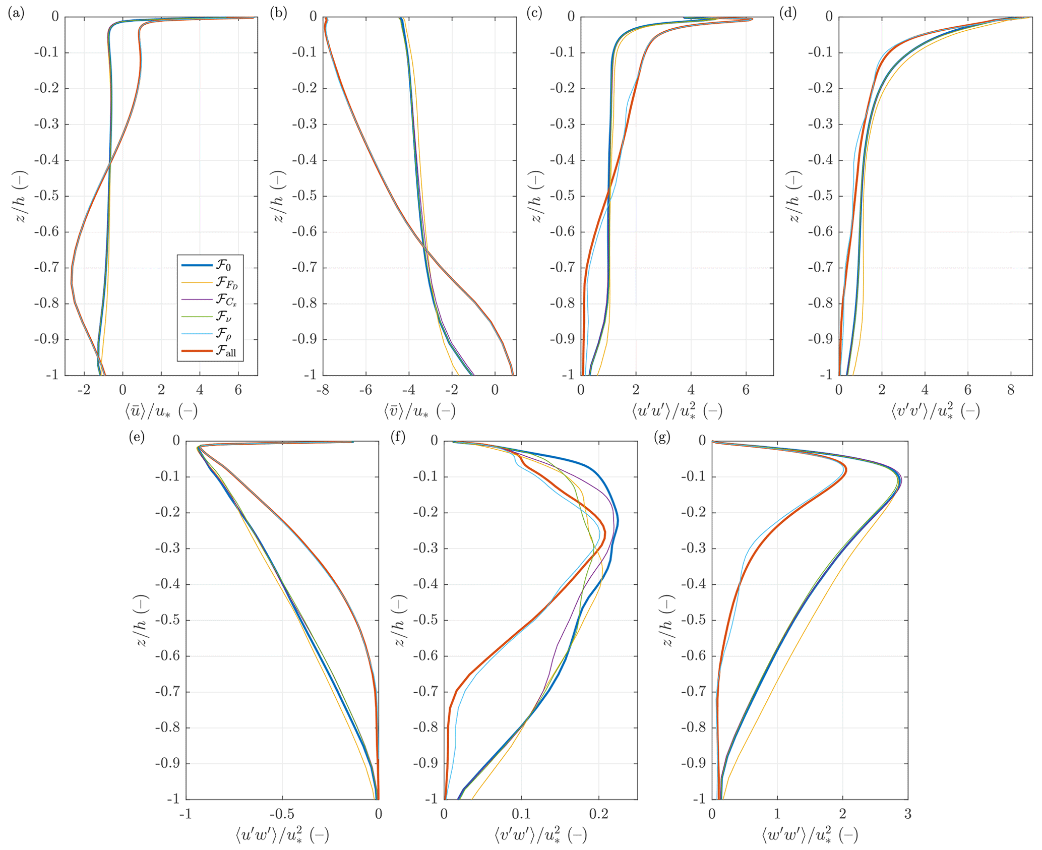
Figure 9 Vertical profiles of the mean velocity (a, b), momentum flux (e, f), and velocity variance (c, d, g) for U_a=30 m s⁻¹ and $T_{\mathrm{a}}=-\mathrm{20}$ ^∘C for all six simulation series. All values are normalized with the respective friction velocity u_*.

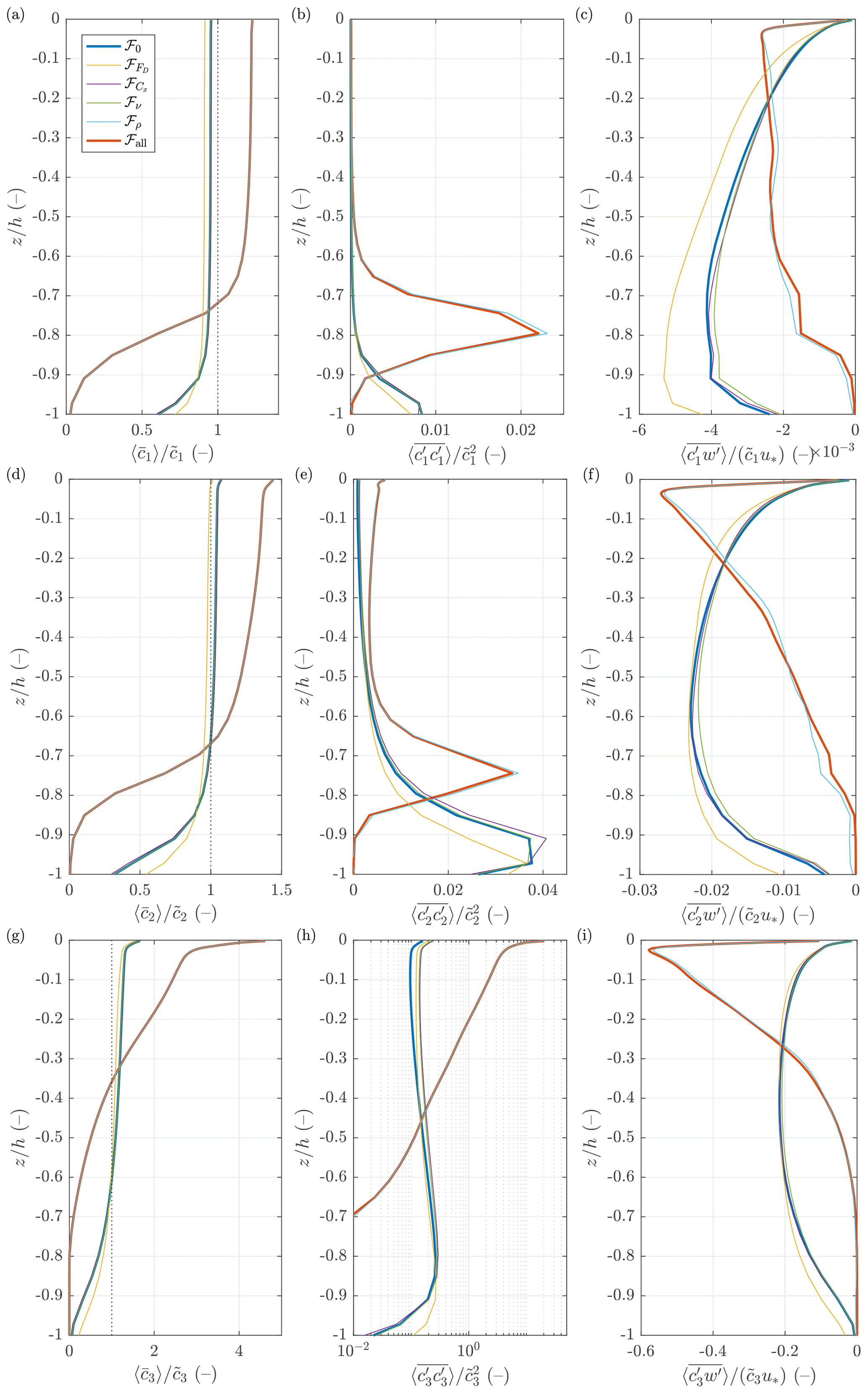
Figure 10 Vertical profiles of the mean (a, d, g), variance (b, e, h), and vertical flux (c, f, i) of the frazil volume fraction for size classes 1–3 for U_a=30 m s⁻¹ and $T_{\mathrm{a}}=-\mathrm{20}$ ^∘C for all six simulation series. Note the different x-axis ranges in the plots; in (h), the x axis is logarithmic.

Figure 11 Direction of the horizontal flow (a) and frazil volume fraction $c_i/{\stackrel{\mathrm{̃}}{c}}_i$ (b–d) along a cross section through the model domain perpendicular to the wind/wave direction (x=600 m in Fig. 12). In (a), a “to” convention is used, i.e., S means the current flowing to the south and so on. In (b–d), black contours show the value of 1. Results of simulations with U_a=30 m s⁻¹ and $T_{\mathrm{a}}=-\mathrm{20}$ ^∘C for series ℱ_all. See Fig. S16 for analogous plots from series ℱ₀.

As expected, in simulations in series ℱ_all and ℱ_ρ, the frazil is concentrated closer to the sea surface. Even in the case of the finest size class, although $\langle \stackrel{\mathrm{‾}}{c_{\mathrm{1}}^{\prime }{c}_{\mathrm{1}}^{\prime }}\rangle$ is small, i.e., the small crystals are uniformly distributed horizontally, ${\overline{c}}_{\mathrm{1}}$ is slightly elevated in the surface layer, and its values drop quickly towards zero at 70–80 m (Fig. 11b); i.e., even the most energetic forcing considered is not sufficient to mix the finest frazil fraction over the entire OML – contrary to series ℱ₀, in which some (small) amounts of frazil are mixed into the pycnocline layer (Fig. S16b). The coarsest fraction (Fig. 11d) is concentrated in the upper portions of the OML and exhibits strong clustering, which is manifested in elevated values of both ${\overline{c}}_{\mathrm{3}}$ and $\langle \stackrel{\mathrm{‾}}{c_{\mathrm{3}}^{\prime }{c}_{\mathrm{3}}^{\prime }}\rangle$ at the surface (Fig. 10). High ice concentration within those clusters, typically with $c_{\mathrm{3}}>\mathrm{10}{\stackrel{\mathrm{̃}}{c}}_{\mathrm{3}}$ (and up to $\mathrm{100}{\stackrel{\mathrm{̃}}{c}}_{\mathrm{3}}$ locally), means that they are also regions of substantially lowered net density. Therefore, it is not surprising that their presence modifies the local circulation in their direct surroundings. Less obviously, important features of the entire OML are affected, which in turn influence the form of the clusters themselves: the frazil streaks are narrower, with larger ice concentration gradients at their boundaries (see color contours in Fig. 12 for an example). The flow in the lower parts of the OML where no coarse frazil is present (below 60–70 m in the case shown in Figs. 11 and 12) is relatively uniform horizontally and directed against the wind/wave direction (note that Figs. 11a and 9 show the Eulerian component of the total velocity without the Stokes drift). In the upper layers, several neighboring zones of different flow directions can be seen, with currents towards S–SE (towards SW–S) correlating with areas of high (low) frazil concentrations, respectively. This relationship between frazil streaks and OML flow can be clearly seen in Fig. 12, in which the anomalies of the vertically integrated velocities are plotted over contours of $c_{\mathrm{3}}/{\stackrel{\mathrm{̃}}{c}}_{\mathrm{3}}$. Frazil streaks are aligned with zones of anomalies directed to, approximately, ESE, and the strongest flow in the opposite direction takes place in regions with the lowest frazil concentration. An interesting feature are anticyclonic (cyclonic) eddies visible to the right (left) of frazil streaks when looking in the downwind direction, separating areas of approximately linearly oriented flow anomalies from each other. Those eddies are small with diameters of ∼100 m and are very different from those present in the results of series ℱ₀ (Fig. S17), which are larger, dominate the depth-averaged flow, and do not have obvious connections with frazil concentration – they mostly reflect the convective circulation spanning the entire depth of the OML, manifested also in the cross sections in Fig. S16. Thus, by modifying the net density, frazil reduces the vertical range of the convective circulation, disturbs the uniform vertical structure of convective cells, and contributes to the formation of organized, relatively regular depth-averaged flow patterns in the OML.

Figure 12 Volume fraction of the largest frazil size class, $c_{\mathrm{3}}/{\stackrel{\mathrm{̃}}{c}}_{\mathrm{3}}$, at the sea surface (color) and anomalies of the vertically integrated horizontal currents (arrows) in simulations with U_a=30 m s⁻¹ and $T_{\mathrm{a}}=-\mathrm{20}$ ^∘C for series ℱ_all. For better visibility, only every fifth arrow in each direction has been plotted.

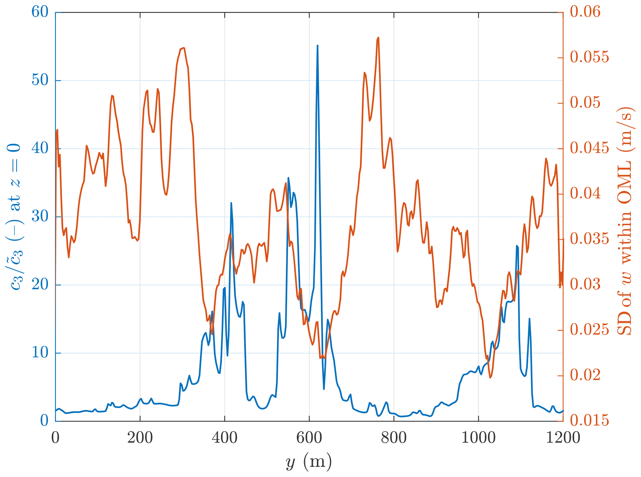
A remarkable difference between the results of series ℱ₀ and ℱ_all is also related to the vertical water velocities. Without frazil→hydrodynamics coupling, as many studies of OML turbulence and material transport have shown (Chamecki et al., 2019), buoyant particles tend to accumulate in zones over the strongest downward currents where the surface convergence is strong. This produces a correlation between positive anomalies of the particle concentration at the sea surface and variance (or standard deviation) of the vertical velocity component w, observed in our series ℱ₀ (Fig. S18). In series ℱ_all, the pattern is very different, as shown in Fig. 13; the most vigorous vertical flow occurs in regions between frazil streaks, and within streaks vertical velocities are significantly reduced, although positive anomalies of c still occur over areas of negative w. In other words, the vertical overturning within streaks is not shut down, but its intensity is reduced. Obviously, this effect might be stronger when the overall ice concentration is higher than considered here.

Figure 13 Volume fraction of the largest frazil size class, $c_{\mathrm{3}}/{\stackrel{\mathrm{̃}}{c}}_{\mathrm{3}}$, at the surface (left axis) and standard deviation of the vertical velocity w within the OML (right axis) in the same situation as shown in Figs. 11 and 12 (section along x=600 m). SD stands for standard deviation.

When analyzing the influence of individual frazil coupling mechanisms, it is worth noting the role of the ice-induced drag in series ${\mathcal{F}}_{F_{\mathrm{D}}}$. In many ways, it is acting opposite to the density-related effects described above; it leads to vertically more uniform velocity and frazil concentration profiles. Its effects are particularly strong in simulations with lower wind speeds and higher air temperatures, when the results of ${\mathcal{F}}_{F_{\mathrm{D}}}$ exhibit less regular circulation cells (and consequently less well-developed frazil streaks) and significantly higher velocity variance $\langle \stackrel{\mathrm{‾}}{u^{\prime }{u}^{\prime }}\rangle$, $\langle \stackrel{\mathrm{‾}}{v^{\prime }{v}^{\prime }}\rangle$, and, especially, $\langle \stackrel{\mathrm{‾}}{w^{\prime }{w}^{\prime }}\rangle$ (not shown).

Finally, coming back to series ℱ_C, x and ℱ_ν, the vertical profiles of scaled quantities analyzed in Figs. 9 and 10 are very similar to those from series ℱ₀, but the domain-averaged momentum and heat transfer between the ocean and the atmosphere are lowered in ℱ_C, x, which leads to generally lower current velocities. The results of series ℱ_ν are sensitive to the total amount of ice present in the OML – the influence of frazil on the net viscosity might be significant when $\stackrel{\mathrm{̃}}{c}$ is larger than in the present simulations.

6 Summary and discussion

As mentioned in the Introduction, the formation of frazil streaks on the sea surface was attributed to the Langmuir circulation already in the first publications on that matter (Martin and Kauffman, 1981; Weeks and Ackley, 1982; Eicken and Lange, 1989). It has remained the “standard” explanation throughout the years, although the arguments supporting it have been of a descriptive, superficial nature and qualitative rather than quantitative – the details of the 3D OML circulation in conditions favorable for frazil formation have been outside of the main focus of sea ice research. To the best of our knowledge, no studies have been devoted to the analysis of size, shapes, and other properties of frazil streaks and their dependence on the wind, wave, and convective forcing. Somewhat ironically, the fact that the observed streaks have irregular shapes and often join with their neighbors has been sometimes used to suggest that Langmuir circulation alone cannot explain their formation and behavior. Progress in research on OML circulation has shown that exactly those features are distinctive of Langmuir turbulence and that Langmuir cells only rarely have regular shapes predicted by the classical theory (Thorpe, 2004). The results of our idealized simulations suggest that, at sufficiently high wind speed, the patterns of frazil concentration at the surface emerge from multi-scale processes, with locally elevated ice concentrations in individual surface convergence zones oriented approximately in the wind/wave direction and larger-scale wide frazil bands oriented obliquely to the wind/wave direction (Figs. 7, 8, 12). Although this result seems to qualitatively agree with observations (e.g., the streaks visible in Fig. 1 are too large and too widely separated to be associated with individual Langmuir cells just a few kilometers offshore, i.e., in a strongly fetch-limited situation), more extensive simulations covering a wider range of parameters (in particular different values of fetch and angle between wind and waves) are necessary to formulate reliable, quantitative hypotheses regarding the spacing and orientation of frazil streaks. Similarly, a different model setting is necessary to analyze the evolution of frazil streaks with increasing distance from the shore, i.e., with spatially varying wave (and possibly wind) forcing. Certainly, observational data are vital in order to test those hypotheses and to confine poorly constrained parameters of the models. In the present simulations, several parameters, e.g., the Prandtl number or the coefficient in the Smagorinsky model of horizontal viscosity, have been set arbitrarily as no data are available that would allow us to determine their “proper” values. Our initial model tests suggest that, in agreement with what is known from LES OML modeling in general, the mean vertical profiles of current velocity and frazil concentration are insensitive to the choice of model parameters, especially those describing subgrid-scale mixing, but the velocity/concentration variance is affected; for example, lowering the Prandtl number leads to slightly stronger clustering of frazil at the surface. Thus, constraining the unknown coefficients is important for the realistic representation of the preferential concentration of buoyant material in the OML.

Even in the idealized model setup used in this study, the number of different combinations of model settings – forcing conditions, coefficients in various (semi-)empirical formulae describing physical processes, alternative mathematical formulations of those processes, etc. – is very large. Therefore, confronted with extremely high computational costs of the model, we were only able to explore a small subspace of the whole multidimensional model parameter space. As described in Sects. 3 and 4, initial sensitivity studies were used to assess the role of some select settings. However, several parameters have been set arbitrarily, and, without further, more extensive simulations supported with observational data, care should be taken when extending the results presented in this paper to conditions outside of the range of those considered here. Also, some formulations used in the new frazil module are well established (or even rather obvious, as is the case of the net density of the ice–water mixture computed from formula 18), while other are based on solutions used in general-purpose mixture models, and their suitability for frazil in the OML remains to be assessed. Moreover, it should be remembered that some of the settings used in this paper are not suitable for simulations with frazil thermodynamics activated. This is certainly true for the number of frazil size classes N_f. Whereas the very small number of classes used here turned out to be sufficient for capturing the processes of interest (initial tests with N_f=10 led to the same conclusions as those with N_f=3), a large number of size classes and a wide range of sizes covered are absolutely necessary to properly simulate the evolution of the crystal size distribution related to thermodynamic processes.

Another serious limitation of the model used in this study, mentioned at the end of Sect. 3.3.3, is related to the formulation of the governing equations, which are valid only for low ice volume fractions. In the simulations discussed above, care has been taken that this assumption has not been violated, but, evidently, this narrows the range of applicability of the model. In the earlier models by Holland and Feltham (2005), Heorton et al. (2017), and De Santi and Olla (2017), the equations are formulated for low ice concentrations as well, but it is assumed that the frazil reaching the sea surface precipitates out of the water column, forming a layer of grease ice at the top of the OML. Moreover, several simplifying assumptions regarding the properties of that layer are made. For example, it has a constant ice volume fraction, and once ice enters that layer, it cannot reenter the water below; i.e., grease ice is in many ways “decoupled” from the rest of the OML. Crucially, no equations describing the motion of that layer are formulated. This approach is acceptable in the 1D settings analyzed in those papers but cannot be transferred to a 3D model setup in which the transient dynamics of a (discontinuous) grease layer and its interactions with the surrounding water have to be taken into account. Thus, multiphase mixture models, valid for an arbitrary number of frazil classes and for $\mathrm{0}\le c_i\le \mathrm{1}$, seem the most appropriate direction in developing future coupled OML and frazil models. Although several elements of the frazil module in our model, including the method of calculating the ice-induced drag force or the net viscosity, are based on methods used in mixture models, it is just a first step towards the proper treatment of the processes and coupling mechanisms involved. It is also worth stressing in this context that some of the effects analyzed here, which turned out to be minor within the range of ice concentrations considered in this study – like, for example, the influence of frazil on the net viscosity – might become relevant at higher ice concentrations.

A very interesting aspect of the results presented in this paper is the “sorting” or de-mixing of an initially uniform mixture of ice crystals of different sizes due to their different floatability. Our results agree with those of Clark and Doering (2009), who observed in a laboratory that small particles were more uniformly distributed in the water column than large ones which tended to exhibit concentration maximum at the surface, especially under low-turbulence conditions. That inherent sorting mechanism might produce several interesting effects when combined with processes not included in the present model version – secondary nucleation, flocculation, crystal growth and melting, and other thermodynamic processes which are affected by the size distribution of crystals. Consequently, it might occur at different rates in surface divergence zones, where only the smallest crystals are present and the total ice volume fraction is relatively low, and in convergence zones, in which the largest crystals accumulate and the width of the crystal size distribution is very wide. It is a subject for subsequent studies to investigate how those 3D dynamic–thermodynamic interactions influence the total frazil production rates and other bulk OML properties and thus whether they should be parameterized in larger-scale models. The same is true for the size-dependent transport of frazil within the OML. As described in the previous section, in coupled simulations (series ℱ_all), frazil streaks form in zones of positive velocity anomalies, coarser frazil fractions are the dominant contributing part of the total ice concentration within those streaks, and, due to their higher floatability, coarse fractions accumulate closer to the surface. Thus, apart from stronger Eulerian currents within streaks, larger ice crystals also experience stronger Stokes drift and as a consequence are transported faster – and in a different direction – than small crystals which are well mixed over the entire OML. This illustrates how the local frazil–hydrodynamics coupling might modify both the bulk behavior of the OML and frazil evolution during frazil and grease ice formation.