the Creative Commons Attribution 4.0 License.
the Creative Commons Attribution 4.0 License.
 | 02 Nov 2020
Sea ice drift and arch evolution in the Robeson Channel using the daily coverage of Sentinel-1 SAR data for the 2016–2017 freezing season
Mohammed E. Shokr
Zihan Wang
Tingting Liu
The Robeson Channel is a narrow sea water passage between Greenland and Ellesmere Island in the Arctic. It is a pathway of sea ice from the central Arctic and out to Baffin Bay. In this study, we used a set of daily synthetic aperture radar (SAR) images from the Sentinel-1A/1B satellites, acquired between September 2016 and April 2017, to study the kinematics of individual ice floes as they approach and then drift through the Robeson Channel. The tracking of 39 selected ice floes was visually performed in the image sequence, and their speed was calculated and linked to the reanalysis 10 m wind from ERA5. The results show that the drift of ice floes is very slow in the compact ice regime upstream of the Robeson Channel, unless the ice floe is surrounded by water or thin ice. In this case, the wind has more influence on the drift. On the other hand, the ice floe drift is found to be about 4–5 times faster in the open-drift regime within the Robeson Channel and is clearly influenced by wind. A linear trend is found between the change in wind and the change in ice drift speed components, along the length of the channel. Case studies are presented to reveal the role of wind in ice floe drift. This paper also addresses the development of the ice arch at the entry of the Robeson Channel, which started development on 24 January and matured on 1 February 2017. Details of the development, obtained using the sequential SAR images, are presented. It is found that the arch's shape continued to adjust by rupturing ice pieces at the locations of cracks under the influence of the southward wind (and hence the contour kept displacing northward). The findings of this study highlight the advantage of using the high-resolution daily SAR coverage in monitoring aspects of sea ice cover in narrow water passages where the ice cover is highly dynamic. The information will be particularly interesting for the possible applications of SAR constellation systems.
- Article
(15474 KB) - Full-text XML
- BibTeX
- EndNote


One of the exit gates for sea ice flux from the Arctic Basin to southern latitudes is through the Robeson Channel. The Robeson Channel is located between Greenland and Ellesmere Island (Canada), with its northern location around 82∘ N, 60.5∘ W (Fig. 1). It connects the Lincoln Sea (a southern section of the Arctic Ocean) to the Kennedy Channel, which opens into the Kane Basin. These three water bodies are known as the Nares Strait, which opens southward to Baffin Bay. The Robeson Channel is a short and narrow passage (about 80 km in length and 30 km wide) that is more than 400 m deep along its axis.
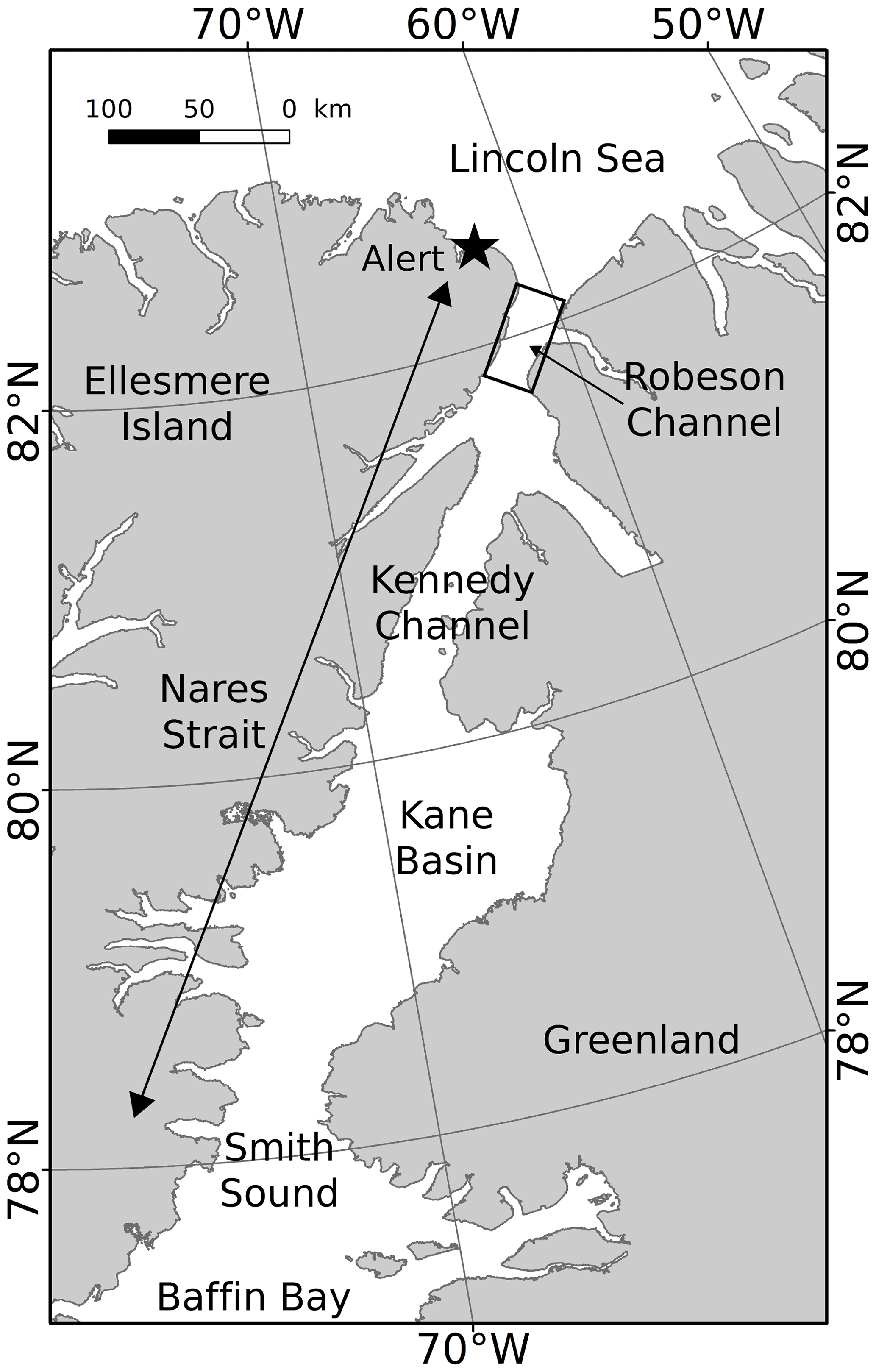
Figure 1Map of the Robeson Channel and its surrounding areas. The Robeson Channel is located between Greenland and Ellesmere Island (Canada), with its northern location around 82∘ N, 60.5∘ W. It connects the Lincoln Sea to the Kennedy Channel, which opens into the Kane Basin.
Oceanographic measurements in the Robeson Channel have not been routinely performed. Herlinveaux (1971) found the dominant surface current to be from north to south in April and May, with an average velocity that increased from about 0.36 km h−1 near the surface to nearly 0.9 km h−1 at a depth of 80 m. A strong southerly current of around 1.08 km h−1 was also measured in the western section of the channel during the early spring of 1971 and 1972, with a standard deviation of 0.43 (Godin, 1979). After using two ocean simulations to study the circulation and transport within the Nares Strait, Shroyer et al. (2015) found that the mean current structure south of the Robeson Channel depended on the presence of landfast ice.
The sea ice cover in the Robeson Channel comprises a combination of seasonal (first-year ice, FYI) and perennial ice (multi-year ice, MYI), both imported from the Arctic Basin through the Lincoln Sea. The only locally grown ice is found in narrow strips adjacent to the land at the two sides of the channel. Based on earlier results for ice thickness and motion retrieved from optical satellite sensors and reconnaissance flights in the 1970s, Tang et al. (2004) estimated the ice flux transiting the Robeson Channel to be around 40×103 km2. Using a record of ice displacement retrieved from RADARSAT-1 images during 1996–2002, Kwok (2005) found the average annual ice area flux to be 33×103 km2. Rasmussen et al. (2010) modelled the sea ice in the Nares Strait using a three-dimensional coupled ocean (HYCOM) and sea ice model (CICE). Their results showed a much lower ice flux in 2006 (20 km3 yr−1) than in 2007 (120 km3 yr−1), which caused blocking of the ice flow in the spring of 2006.
Sea ice drift is influenced by wind forcing, ocean currents and internal stresses within the pack ice. Internal stresses, which are caused by the interactions between ice floes and determined by the ice types and concentrations within the pack, reduce ice momentum. Other minor factors include the Coriolis force and sea surface tilt. The dynamics of the ice motion can be assessed at a variety of spatial and temporal scales (McNutt and Overland, 2003), namely individual-floe (< 1 km), multiple-floe (2–10 km for up to 2 d), aggregate-floe (10–75 km with a 1–3 d timescale), pack ice cover (75–300 km at 3–7 d) and sub-basin (300–700 km at 7–30 d) scales. The best coupling with wind occurs at the pack ice scale (also called the coherent scale). According to this categorization, only the individual- and multiple-floe scales can be observed in synthetic aperture radar (SAR) images of the Robeson Channel. In this case, the response to wind is usually manifested in floe-to-floe bumping, causing ridging, fracturing, floe breaking, re-orientation and differential motion (McNutt and Overland, 2003).
Tracking individual ice floe motion from a sequence of satellite images is potentially feasible if the temporal resolution of the satellite coverage is sufficient (at least daily). An early attempt was reported in Sameleson et al. (2006) for ice in the Nares Strait using coarse-resolution satellite data (tens of kilometres) from a passive microwave radiometer at 6.5 GHz. The authors tracked the motion using only three to five locations of the same ice floe in a sequence of satellite images. Vincent et al. (2001) used Advanced Very High Resolution Radiometer (AVHRR) data (with frequent passes in the polar region) to track the motion of the ice floes in the Nares Strait. However, due to the coarse resolution of the sensor, the results did not demonstrate the motion of individual ice floes.
Due to their fine resolution (tens of metres), sequential SAR images are the best tool to monitor sea ice kinematics, particularly if available at a short timescale. However, SAR data have a limited spatial coverage. The earliest studies to estimate sea ice displacement using SAR data were presented in Hall and Rothrock (1981) and Leberl et al. (1983), using sequential SeaSat SAR images. Later, making use of the more frequent coverage of RADARSAT-1 in the western Arctic, the RADARSAT Geophysical Processing System (RGPS) was developed and produced gridded ice motion and deformation data, tracked every 3–6 d from 1998 to 2008 (Kwok and Cunningham, 2002). A more recent ice tracking operational system (also gridded) was described in Demchev et al. (2017), using a series of Sentinel-1 SAR images.
While the Robeson Channel is covered most of the year by an influx of ice from the Lincoln Sea, the flow of the ice is sometimes blocked in the winter at the entrance of the channel by the formation of an arch-shaped ice configuration that spans a transect between two land constriction points at Greenland and Ellesmere islands. The arch usually collapses in early summer, allowing continuation of the ice flux. Kwok et al. (2010) pointed out that no arch was formed in 2007, leading to a major loss of Arctic ice, which was equivalent to about 10 % of the average annual amount of ice discharged through the much wider Fram Strait (400 km versus 30 km width). This signifies the fact that the entire Nares Strait could represent a major route to the Arctic if the ice arch ceases to form in the future due to the thinning of Arctic ice. Moore and McNeil (2018) addressed the collapse of this arch in relation to the recent trend of sea ice thinning. In this study, the arch formation started on 24 January 2017 and continued until May 2017. The paper includes a detailed description of the mechanism of the arch's development.
The objective of the study was to utilize the daily Sentinel-1A/1B SAR coverage of the Robeson Channel area during a full freezing season (September 2016 to end of April 2017) to examine two sea ice process mechanisms in the Robeson Channel. The first was the drift of individual ice floes, in terms of speed and direction. For this purpose, 39 ice floes were selected and each floe was tracked manually in the series of available Sentinel-1 images. The motion information was linked to the 10 m wind reanalysis data to explore the influence of wind on the ice drift. When wind did not explain the ice motion, an explanation in terms of other factors, namely ocean current, surrounding ice concentration, tidal forces and to a much lesser extent the sea surface height (SSH), was considered. Knowledge about how wind and ice drift are related enables the improvement of sea ice–atmosphere dynamic models (Leppäranta, 2011). The second process was monitoring the development of the ice arch at the inlet of the Robeson Channel during its development until maturity. The advantage of using the daily coverage of the fine-resolution SAR data in retrieving this information in such a narrow channel is expected to instigate further operational applications of SAR constellation systems (e.g. the recent Canadian RADARSAT Constellation Mission (RCM)) with their finer temporal resolutions. It should be noted that operational ice drift products are generated based on cross-correlation between sequential images, which is a statistical approach, while the current approach is based on the manual identification of individual ice floes. Admittedly, this task is laborious, but the motion product has a superior accuracy and can be linked to a detailed dataset of reanalysis wind.
2.1 Satellite data
Sentinel-1A and 1B are two satellites developed within the satellite constellation of the European Space Agency's (ESA) Copernicus programme. They were launched on 3 April 2014 and 25 April 2016, respectively. Both carry a carbon-copy C-band SAR sensor (with a central frequency of 5.405 GHz) with a selection of single or dual polarization. Image acquisition is performed in one of four operation modes: stripmap (SM), interferometric wide swath (IW), extra-wide swath (EW) and wave (WV). The IW (swath width 250 km at a spatial resolution of 5 m × 20 m) and EW (swath width 400 km at a median resolution of 20 m × 40 m) modes were used in this study, which are both Level-1 Ground Range Detected (GRD) products. All the images were acquired in HH polarization. An almost daily coverage of the Robeson Channel area from both satellites was obtained from late September 2016 to the end of April 2017 (a total of 361 images). The images were calibrated to give backscatter coefficients in decibels and were then georeferenced. In order to reduce the image size and the speckle, the images were resampled to 50 m × 50 m. While the incidence angle of the EW mode varies between 29.1 and 46.0∘ across the swath, no correction for the variation in the angle was performed since the backscatter was not used quantitatively.
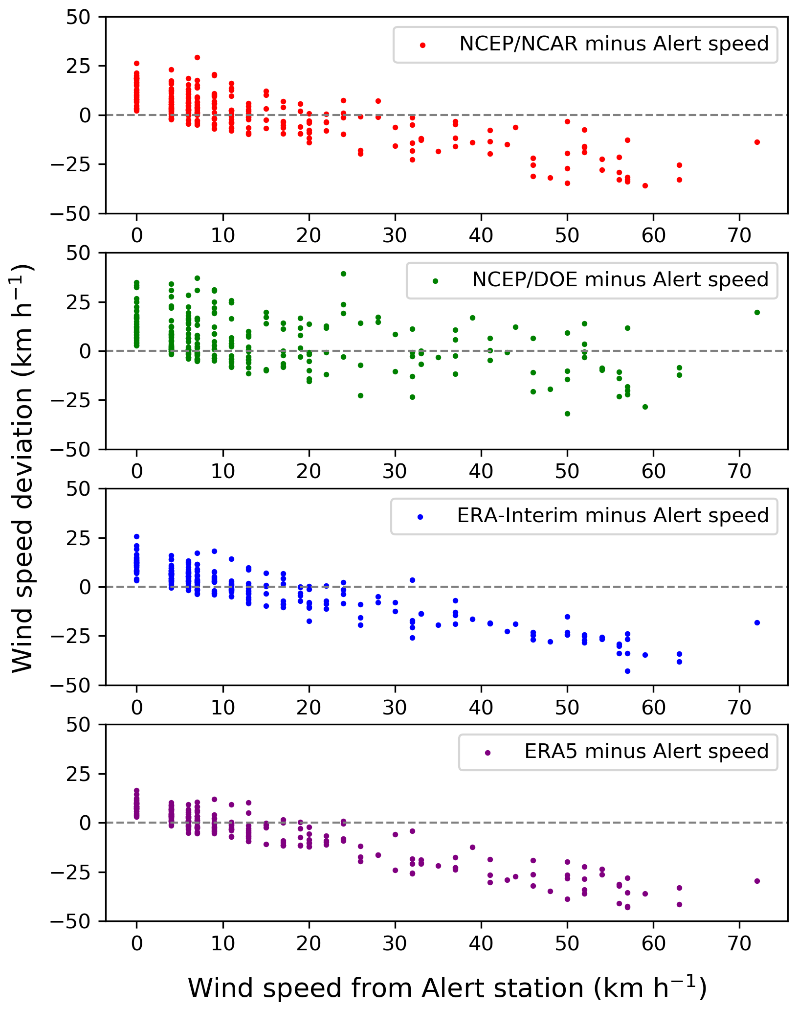
Figure 2Deviation of the reanalysis wind speed from the speed measured at the Arctic Alert weather station (reanalysis wind minus station wind) for the period 1 October 2016 to 30 April 2017. The reanalysis data are from NCEP/NCAR, NCEP/DOE, ERA-Interim and ERA5. Note the increasing underestimation of the reanalysis data as the measured wind increases. Units of the x axis in the bottom segment apply to all segments.
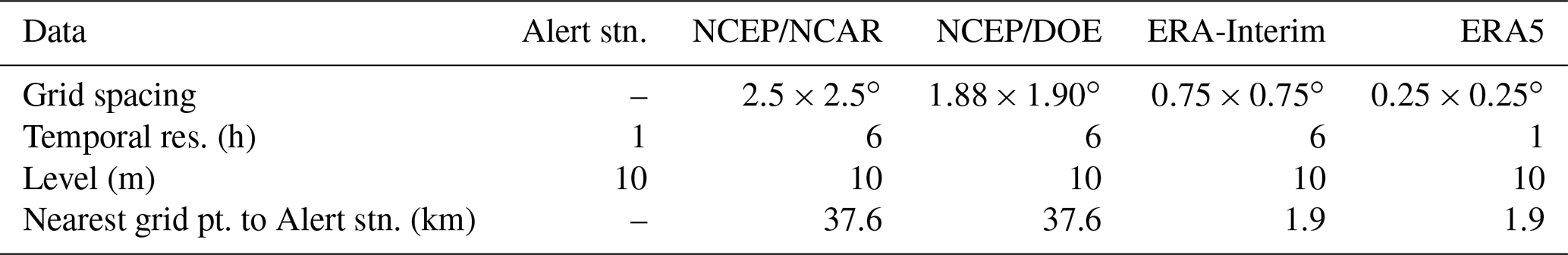
Table 1Information about the available wind data for the study area from the Arctic Alert weather station and the four sources of reanalysis data.
2.2 Wind data
Reanalysis of 10 m level wind is available from a few sources. Four sources were examined in this study: (1) the US National Centers for Environmental Prediction/National Center for Atmospheric Research (NCEP/NCAR) reanalysis project (Kalnay et al., 1996), (2) the NCEP/Department of Energy (NCEP/DOE) reanalysis model (Kanamitsu et al., 2002), (3) the European Centre for Medium-Range Weather Forecasts (ECMWF) reanalysis (ERA-Interim) (Dee et al., 2011) and (4) its successor ERA5 (C3S, 2017). The specifics of each source are presented in Table 1. The difference between the estimated speed from each source and the speed from the Arctic Alert station is plotted in Fig. 2 for the period from 1 October 2016 to 30 April 2017. The Arctic Alert weather station (Canada) is located at 82.52∘ N, 62.28∘ W. This location is reasonably close to the Robeson Channel and is thus the best ground source to characterize the general wind field at a temporal resolution of 1 h (Fig. 1).
Figure 2 reveals the overestimation of the reanalysis wind when the station's wind measurement is < 10 km h−1. As the wind measured from the station increases, a systematic underestimation of the reanalysis wind can be observed. This is particularly true of the two ERA products. When the speed from the Alert station exceeds 30 km h−1, the reanalysis wind from all sources can be severely underestimated by as much as 20–40 km h−1. Previous studies have shown that the low-resolution global reanalyses of the wind speed and direction have large errors in the narrow channels of the Nares Strait (Dumont et al., 2009). The present data show that the average absolute deviation of the NCEP/NCAR, NCEP/DOE, ERA-Interim and ERA5 wind reanalysis from the measured wind at the Alert station is 9.12, 9.74, 9.04 and 8.92 km h−1 over the period from 1 October 2016 to 30 April 2017. Hence, we chose the ERA5 data because of their minimum deviation from the Alert station data and the finer grid spacing. The data were used to explore links with the ice floe drift and to study the ice arch development. The grid points from the ERA5 reanalysis relevant to the study area are shown in Fig. 3. Data from the appropriate grid points are introduced later in the relevant sections.
2.3 Ocean current and sea surface height (SSH)
Daily and monthly mean maps of ocean current (vertical coverage at 50 levels from −5500 m depth to surface) and SSH are components of the GLORYS12V1 reanalysis product covering the satellite altimetry era (1993–2018). This is based on the real-time ocean reanalysis product of the Copernicus Marine Environment Monitoring Service (CMEMS) (Fernandez and Lellouche, 2018; Lellouche et al., 2018). The maps were generated at a spatial resolution of 1/12∘ × 1/12∘, and both parameters were used to support the interpretation of the ice floe drift when it could not be explained by wind data only.
The daily fine-resolution images of Sentinel-1A/1B (50 m) were used to generate tracking of the selected sea ice floes and to detect the temporal evolution of the ice arch from its commencement on 24 January until it matured on 1 February 2017. In total, 39 ice floes were tracked between 26 September 2016 and 11 April 2017. A total of 32 ice floes moved mainly southward, crossing the inlet of the Robeson Channel, and seven moved mainly northward within the Robeson Channel. Among the seven ice floes, five moved in the drifted ice regime before and shortly after the formation of the ice arch, and two moved into a polynya-like regime after the formation of the arch. Each ice floe was visually identified in a sequence of daily SAR images (between 11 and 54 sequential scenes), and then the ice floe displacement, drift speed and direction were calculated. The displacement was determined from the subjectively estimated locations of the same ice floe in two successive daily images, using a code to convert latitude–longitude pairs to distance according to the World Geodetic System (WGS84) coordinate system.
Three sources of error were implied in the estimation of the displacement. The first was the geolocation error of the SAR imagery. The Sentinel-1 product specification (Bourbigot et al., 2016) mentions that the absolute pixel location accuracy is less than 7 m for the IW mode, but no figure is given for the EW mode, which was used in this study. The second source of error was the assumption of a linear path (as opposed to a curvilinear or meandering path) for the ice floe between 2 successive days. This assumption had to be employed because the temporal resolution of Sentinel-1A/1B is not finer than 1 d. The pattern of ice floe motion depends primarily on the changing wind direction and the mechanical properties of the surrounding ice floes. The third source of error was the subjective estimate of the centroid of the same ice floe in successive images. This was also estimated to be within a few pixels. Assuming that these errors were independent and normally distributed, the error in the estimated ice drift speed would be roughly 0.2 km d−1.
The ice floe speed was calculated using the travelled distance, as mentioned above, and the period between the two successive image acquisitions, which varied between 16 and 33 h. To link the ice floe speed to the wind at any ice floe location, the reanalysis wind values from ERA5 for the four grid points closest to the floe were averaged. This was done to avoid the inclusion of wind data from grid points far from the relevant ice floe location, which can often be very different. The 3 h wind vectors that acted on the given ice floe during its transition in the period of the two satellite passes were produced in the form of polar maps, to qualitatively explore their influence on the ice floe drift. In addition, the 3 h wind speeds from the four grid points around each ice floe at each location were averaged to quantitatively link to the drift speed. Statistics were then generated to quantify the wind influence.
The evolution of the ice arch from its onset of formation on 24 January until its maturity on 1 February 2017 was manually delineated in each image. The daily displacement of the two end points of the ice arch was calculated using the latitude–longitude coordinates. To investigate the role of the wind in the progress of the arch shape, as well as the location and displacement of its terminal points, daily wind data from the ERA5 reanalysis were averaged from the 3 h intervals at the coloured grid points from lines 3, 4 and 5 (corresponding to latitudes 82.5, 82.25 and 82∘ N, respectively) in Fig. 3.
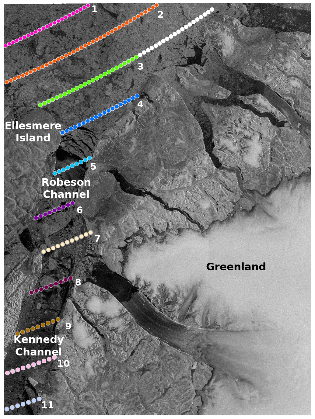
Figure 3ERA5 grid points of the wind reanalysis data used in the present study. The background is the Sentinel-1B image acquired on 30 January 2017.
The ice floe motion and arch formation are addressed in two subsections. The ice floe motion is considered in two separate regimes: north of the Robeson Channel near its entrance and within the Robeson Channel. In the first regime, the ice floes approach the Robeson Channel in a convergent path forming pack ice cover, which is a term used when ice concentration exceeds 70 %. On the other hand, the ice regime within the Robeson Channel falls into the category of drifted ice, a term used to denote an ice concentration of less than 60 %. The two regimes feature different ice floe drift patterns, and the influence of the wind also differs, as explained later. Case studies of the ice floe motion are presented for each regime to reveal the quantitative and qualitative information about the wind influence. In the second subsection, the role of the wind in the evolution of the ice arch at the inlet of the Robeson Channel is addressed.
4.1 Ice floe motion
4.1.1 Tracking ice floe drift
The ice flux transiting the Robeson Channel encompasses ice floes of different ages and sizes. The typical dimensions of the ice floes examined in this study ranged from 2 to 16 km. Some ice floes were aggregates of smaller floes, which disintegrated during their journey. The 39 ice floes selected for motion tracking in the Sentinel-1 images were numbered, and the numbers are used in the following analysis, although the order does not carry any significance. The tracks of 12 ice floes are shown in Fig. 4, with the floe numbers and the dates at each position attached. These ice floes were mostly heading southward, but with a few interruptions to this dominant direction. The high ice concentration in the convergent path upstream of the Robeson Channel caused reduction of the ice motion and induced meandering paths. However, in areas with less ice concentration, the ice floe motion accelerated and became more influenced by wind, as will be demonstrated in case study 1. Once the ice floes crossed the bottle neck at the entrance to the Robeson Channel, they became partially relieved from the stresses induced by the surrounding ice and more responsive to other factors such as wind and current. Thus, the speed increased greatly by a factor of 1.5–5, and the drift direction followed mostly the north–south extension of the Robeson Channel, which coincided with the dominant wind direction. This direction also coincided with the dominant ocean current direction. Figure 4 also shows that the ice floes did not enter any of the fjords at the sides of the channel. In fact, many fjords become filled by locally grown landfast ice early in the freezing season.
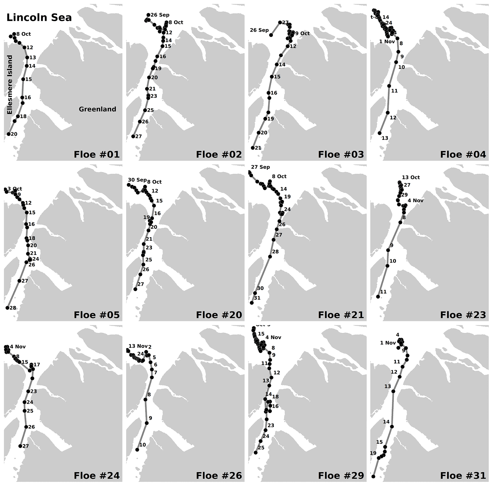
Figure 4Trajectories of 12 selected ice floes, obtained from the daily Sentinel-1 images, as they approach and pass through the Robeson Channel. Note the slow motion upstream of the channel and the faster motion through the channel. The entrance to the channel is marked by the solid line in the top left panel.
4.1.2 Ice floe drift speed
Figure 5 shows the average drift speed of each ice floe (regardless of drift direction) during its entire observation time in the SAR time series, either upstream or within the Robeson Channel. Upstream of the Robeson Channel, the drift speed varied within a narrow range (4–10 km d−1), with a typical value around 5 km d−1. Such nearly constant drift speeds, observed under different wind speeds, suggest that the wind has a minor influence or even no influence on the ice floe drift in this area. The exceptionally high average speed of ice floe no. 6 (∼ 19 km d−1) resulted when the floe drifted in a surrounding area of nearly zero ice concentration, which prevailed for 3 d.
The situation was different for the ice floes that drifted within the Robeson Channel. Here, the ice floe speed was much higher, typically between 14 and 45 km d−1. One ice floe reached an extreme speed of around 99 km d−1 on one day, as shown in case study 3 below. The higher drifting speed inside the Robeson Channel can be partly explained by the low ice concentration and/or the prevalence of thin ice, particularly after the ice arch matured on 2 February 2017. Both factors gave rise to a more significant influence of wind and ocean currents on the ice drift. The large variability of the ice floe speed within the Robeson Channel, which contrasts with the nearly constant speed upstream of the Robeson Channel, can be attributed to the influence of the variable wind speed and direction. For example, the very high average speed of ice floe no. 4 (45 km d−1, as shown in Fig. 5), which is a manifestation of the large leap in location during the period 10–13 November (Fig. 4), was instigated by a dominant southward wind between 20 and 40 km h−1 during that period. On the other hand, the relatively slow average drift speed of ice floe no. 5 (15 km d−1, as shown in Fig. 5) resulted from a reversed wind direction that blew from south to north at 10–20 km h−1 between 18 and 26 October. This adverse wind neutralized the action of the southward current.
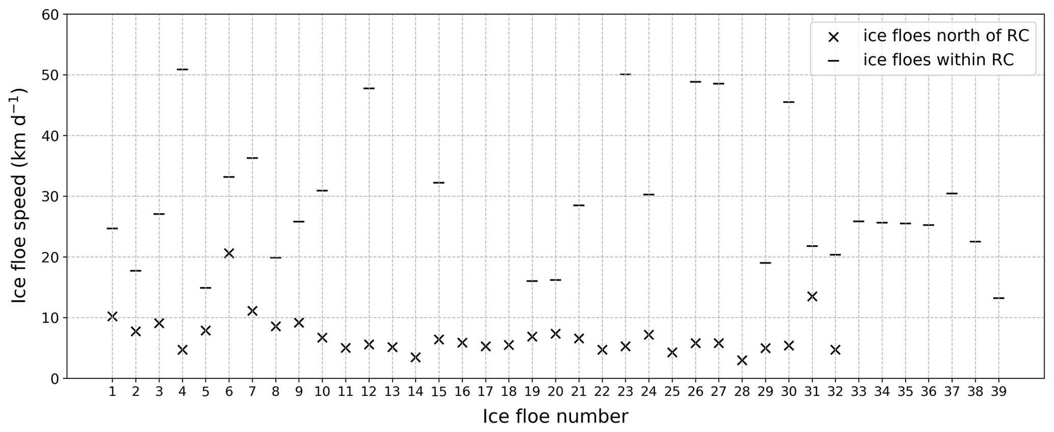
Figure 5Average speed of individual ice floes during the periods upstream and within the Robeson Channel. The last seven floes (nos. 33–39) drifted within the Robeson Channel with highly variable speeds.
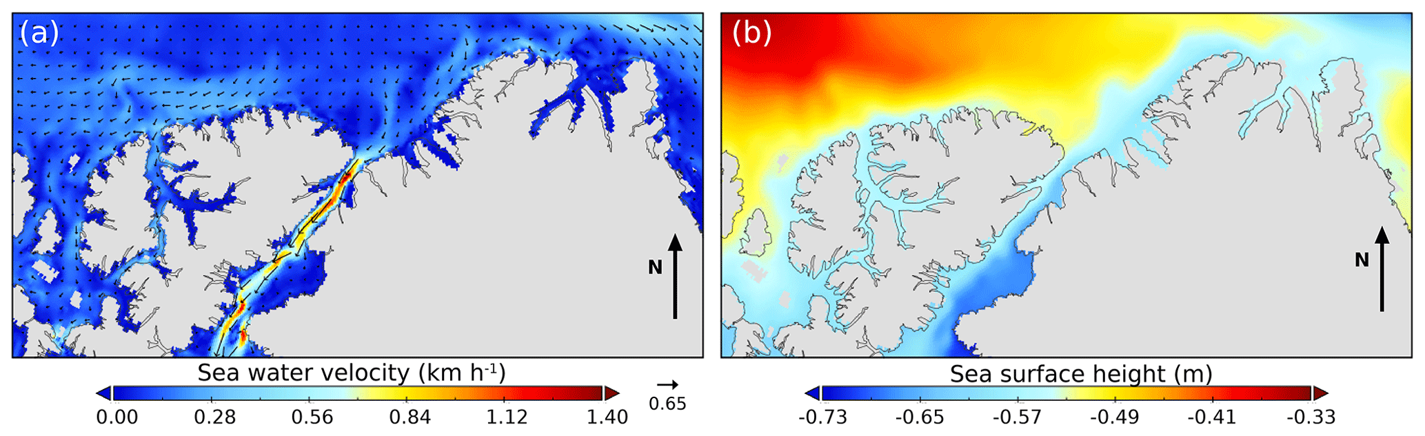
Figure 6Maps of ocean current near the surface (a) and sea surface height (b), averaged over December 2016 from GLORYS12V1, which is generated by the Copernicus Marine Environment Monitoring Service.
4.1.3 Driving forces of ice floe motion
While several studies have confirmed the coherency between wind forcing and the large-scale motion of pack ice, the results presented in this section are focused on examining the influence of wind on the drift of individual ice floes. For the large-scale motion of the pack ice in the Nares Strait, Kwok et al. (2013) confirmed that this was triggered by both ocean current and wind, which pushed the ice from the Lincoln Sea southward to the Robeson Channel. As mentioned in Sect. 1, ice dynamics at the individual-floe and multiple-floe scales is triggered by a combination of wind, ocean current, internal stress within the pack ice, the Coriolis force, SSH and tidal forces. In the following presentation, when the wind is not found to be linked to the observed ice motion, other factors are considered. A few points about some of these key factors are reviewed here.
Ice concentration is used as a proxy indicator of internal forces within the pack ice. In this study, this parameter was visually estimated from the SAR images. In close pack ice (ice concentration > 70 %), the influence of the internal forces overrides other factors such as wind and current, as shown in case study 1. On the other hand, when ice moves in a drifted ice regime with a low ice concentration, which is the case within the Robeson Channel, the effect of the wind and ocean currents becomes more pronounced. As mentioned above, the maps of ocean currents and SSH are available from the same source in daily and monthly average gridded products. An example of the monthly averaged data for December 2016 is shown in Fig. 6. This example is typical of the winter months. The surface current in the central path of the Nares Strait, including the Robeson Channel, is about 5 times faster than the typical current north of the Robeson Channel, and the dominant southward wind reaches speeds between 0.72 and 1.38 km h−1. This would be powerful enough to influence the ice floe drift. We performed multivariate regression analysis using the current and wind data from within the Robeson Channel to evaluate the relative weight of each factor. The SSH map for December 2017 (Fig. 6) reveals a decreasing gradient westward. This might suggest a limited impact on the ice floe motion, particularly north of the Robeson Channel (Wekerle et al., 2013).
Tide data in this region are not generated regularly. A few datasets are available, which were acquired during expeditions to measure other oceanic parameters. For example, Münchow et al. (2007) and Münchow and Melling (2008) measured ocean currents in the Nares Strait using mooring buoys, most of which were located at the southern end of the Kennedy Channel. They found that the tide impacted the dominant component of current in the Nares Strait. However, Münchow et al. (2007) indicated that the amplitude and phase of the tidal constituents varied substantially both along and across the strait. Meanwhile, Johnson et al. (2011) indicated that Petermann Fjord, at 81∘ N, is well above the critical latitude for the M2 tide (74.5∘ N). Since the Robeson Channel is above the latitude of Petermann Fjord, the tidal effect is assumed to have a much smaller influence on ice drift in the Robeson Channel than the other regimes in the Nares Strait. Gimbert et al. (2012) used the Fourier spectra of the buoy velocity from the International Arctic Buoy Programme (IABP) to investigate the impact of the tidal effect in the Arctic Basin. We checked all the available buoy datasets and found that nine buoys operated in the Nares Strait during September to April, from 1979 to 2016. We calculated the Fourier spectra of the velocity records from each buoy and found different spectra from the different buoys, some with and others without peaks. The peaks may be linked to the regular pattern of the tide. Therefore, no confirmed conclusion could be obtained from this dataset on how tide impacts ice drift in the Robeson Channel.
Ice drift upstream of the Robeson Channel
Synoptic information about the ice regime north of the Robeson Channel is presented using the six selected scenes shown in the sequence of Sentinel-1 images in Fig. 7. A bulge-shaped area of consolidated ice appears to be attached to the coast of Greenland. It is delineated by the dotted lines in all the images, except in the image for 26 October, although it is still just visible in this image. This may possibly be a large extent of landfast ice, although it was exposed to cracking, as can be seen in the image for 7 November. An arch-like crack is visible in the image for 13 November, with its boundary coinciding with the bottom boundary of the landfast ice area. This was probably instigated by the strong southward wind (20–60 km h−1) which prevailed on 8 November. However, this arch did not survive because its west-side terminal (left side in the image) was not anchored on land at this point. Further details of this phenomenon are presented in the next section.
Figure 7 shows that the ice entering the Robeson Channel follows a path coming around the north of Ellesmere Island, as shown by the arrow in the image for 1 December. No ice appears to be coming along the coast of Greenland. This large-scale motion is likely driven by the strong southward wind, which is channelled down the atmospheric pressure gradient from the Lincoln Sea to Baffin Bay (Gudmandsen, 2000), and the ocean current. However, since the ocean current is very weak in this area (Fig. 6), it is possible that the ice motion around the tip of Ellesmere Island is driven by the west–east gradient of the SSH (Fig. 6). Wekerle et al. (2013) mentioned that the SSH difference between the Arctic Ocean and Baffin Bay not only leads to a net outflow from the Arctic Ocean, but its variability also drives the variation in the Canadian Arctic Archipelago (CAA). As the ice cover approaches the entrance of the Robeson Channel, the ice floes demonstrate erratic motion (Fig. 4). This nullifies the possible influence of ocean current or SSH. The ice floe motion immediately upstream of the Robeson Channel appears to be mainly determined by the interactions between neighbouring ice floes in the closed pack ice. This observation is illustrated in the following case study.
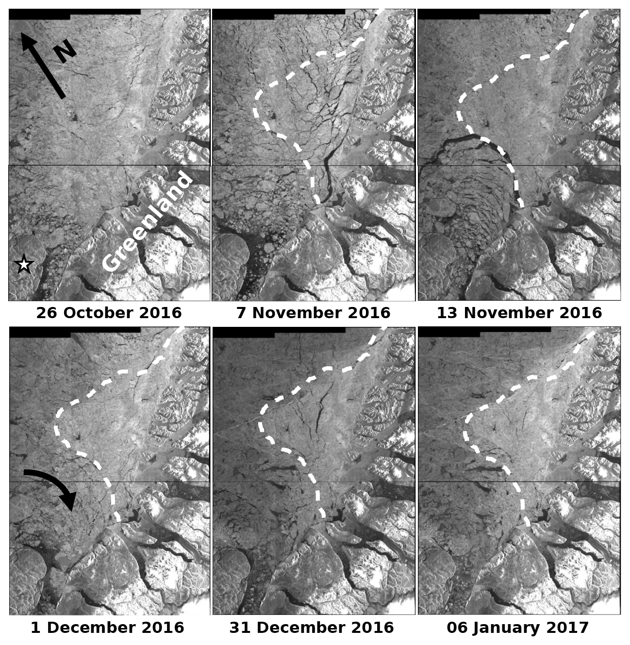
Figure 7Sequence of Sentinel-1A/1B images for an area north of the Robeson Channel. The dotted curve marks an area of consolidated ice (still visible in the 26 October image). Ice cracked in this area on 7 November and an ice arch was formed on 13 November. The star in the middle panel of the top row marks Ellesmere Island. Ice floes that made their way to the Robeson Channel originate from the west (not north), following the path shown by the arrow in the 1 December image.
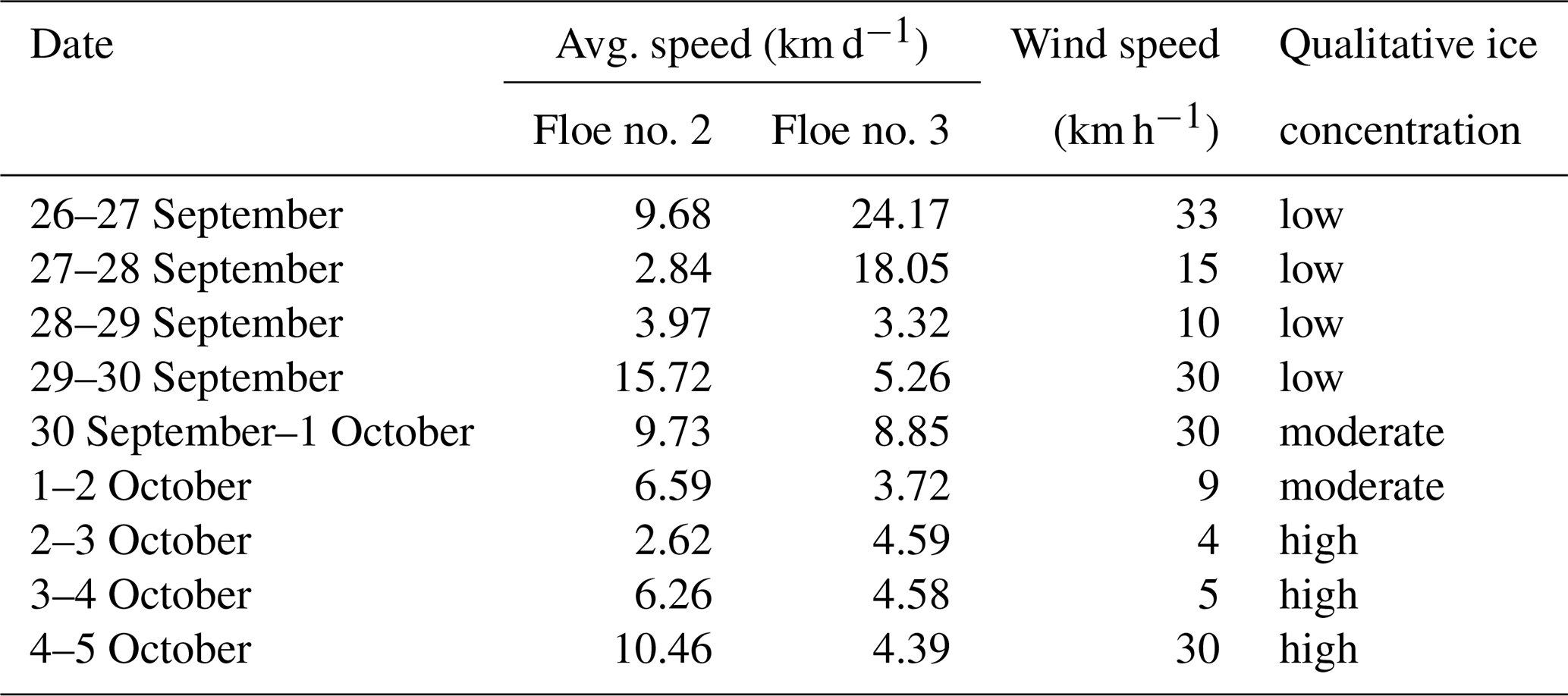
Table 2Drift speed of ice floe no. 2 and no. 3 (shown in Fig. 8) during the period between the acquisitions of the two successive daily Sentinel-1 images. The period is shown in the first column.
Case study 1: two floes drifting upstream of the Robeson Channel
Figure 8 shows sequential Sentinel-1 images (26 September to 7 October 2016) of a segment just upstream of the Robeson Channel, where two ice floes appear. Ice floe no. 2 is marked by the grey dot, a natural low-backscatter area, and floe no. 3 is marked by the star. The corresponding maps of the 3 h ERA5 reanalysis wind vectors are presented in Fig. 9. The daily speeds of each ice floe are listed in Table 2, along with the wind and qualitative concentration data. This information helps in defining the impact of the wind on the ice floe drift, as explained below.
The image for 26 September shows the two ice floes surrounded by open water and thin ice. The wind between the two satellite overpasses on 26 and 27 September (averaging 33 km h−1) was partly heading northeast or southeast. This relatively high wind, combined with the less resistive ice in the surroundings, caused floe no. 3 to drift northeast at a top speed of 24 km d−1 (Table 2). Between 27 and 28 September, relatively light wind (< 20 km h−1) blew in the opposite direction, but floe no. 3 drifted southeast at 18.05 km d−1 because this path was the path of less resistance. Floe no. 2 did not move far with a drift speed of 2.84 km d−1 as it was surrounded by ice. Between 28 and 29 September, the light wind did not change and the two ice floes remained at the same locations. When the wind direction switched to the southeast between 29 and 30 September, with the speed reaching 30 km h−1, the two floes drifted in the same direction, with floe no. 2 reaching a speed of 15.72 km d−1, as shown in Table 2. Here, once again, the path was nearly ice-free. Between 30 September and 1 October, when a southwestward wind blew at nearly 30 km h−1, the ice drift accelerated to nearly 9 km d−1. After 1 October, the wind abated but the drift continued in a southeast direction at a moderate speed of 2–6 km d−1. When the northward wind exceeded 40 km h−1 between 4 and 7 October, before it was reduced to less than 30 km h−1, the ice floe drift did not follow the wind action in the first 2 d because the two floes were surrounded by high ice concentrations. Nevertheless, southwestward drift was observed between 4 and 5 October, particularly for floe no. 2 (Fig. 8), following the strong northwestward wind during the same period (Fig. 9). This case study demonstrates the effective role of wind on ice floe drift when the floe is surrounded by thin ice or water.
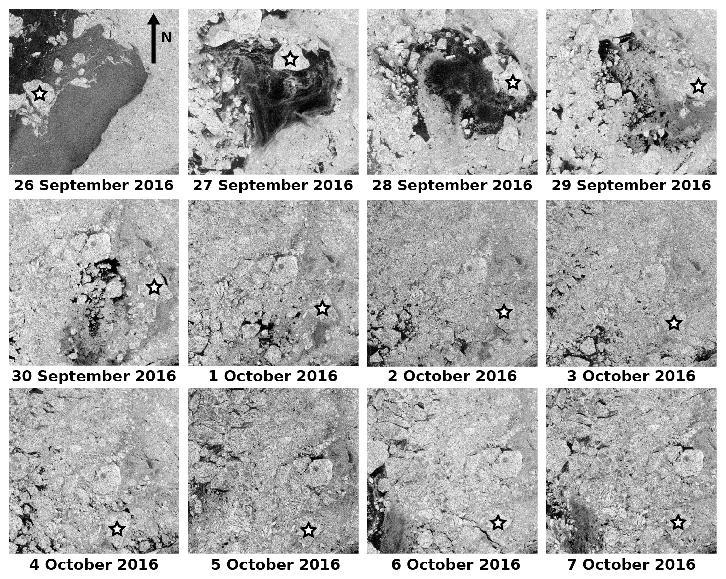
Figure 8Sequential Sentinel-1A/1B images (dates are shown) showing the advancement of two ice floes. Floe no. 2 is marked by a grey dot (a natural low backscatter area), and floe no. 3 is marked by a star. The ice concentration surrounding each floe is visible and can be qualitatively estimated.
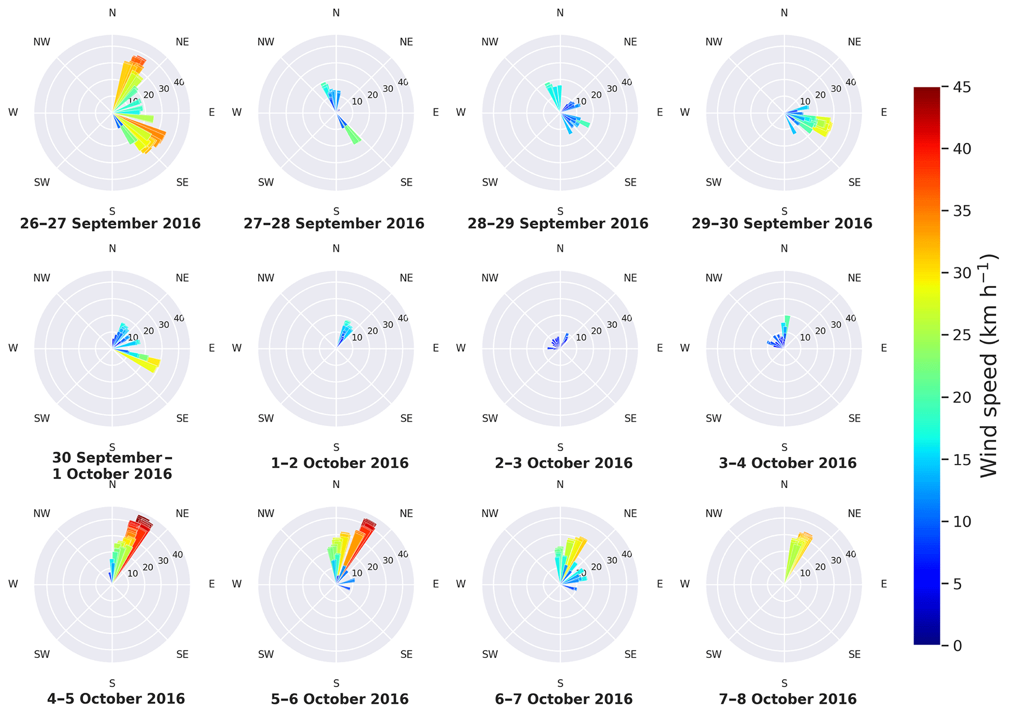
Figure 9Maps of the 10 m level wind vector (km h−1) from the ERA5 reanalysis. Each panel has vectors from the four grid points surrounding the locations of ice floe no. 2 and no. 3 every 3 h during the time between the daily overpasses of Sentinel-1. For example, the 26–27 September panel shows the 3 h vectors that were available between the period that spans the satellite acquisition times of 26 and 27 September.
Ice drift within the Robeson Channel
Prior to the formation of the ice arch on 24 January 2017, the channel was filled with ice floes transported from the north. Shortly after the development of the ice arch, the channel became covered with thin ice and open water, which is typical of polynya cover. In both situations, the direction of the ice floe motion was mainly north–south, following the dominant wind and current directions, although the wind was occasionally reversed (Fig. 4). The low ice concentration (< 40 %) in this drifted ice regime enhanced the roles of all the factors impacting the ice motion, particularly the wind and ocean current. In the absence of other factors, the role of the wind is examined through the scatter plot of the wind and ice motion components in the north–south direction, as shown in Fig. 10. The data points marked by the open circles in Fig. 10 represent floe numbers 1–37, which entered the Robeson Channel from the north prior to the arch formation, and the points marked by the closed circles are from the motion of floe no. 38 and no. 39. These two floes originated in the Robeson Channel after the arch formation, so they moved freely in the thin ice/water field. Positive values indicate motion northward, and vice versa. It can be seen that a southward-blowing wind is always associated with southward ice drift. When the wind blows northward, the ice floes may remain drifting southward. In this case, the motion must be influenced by the southward ocean current. However, as the northward wind accelerates, the ice may eventually drift northward. This is shown in the reversed path of floe no. 29 between 10 and 18 November in Fig. 4.
The trend of the data points in Fig. 10 is defined by the linear regression equation , where fs and ws are the ice floe and wind speed, respectively. The slope of the regression line from the data of floe nos. 1–37 (Fig. 10) shows that when the ice floe motion coincides with the wind direction, the flow speed becomes roughly 1∕15 of the wind speed. This equation suggests that, in the absence of wind, the ocean current would induce floe drift (southward) at approximately 0.98 km h−1 (22 km d−1). The coefficient of determination (R2) of this regression is 0.565. The same coefficient increases to 0.679 from the data for floe no. 38 and no. 39 only. A higher R2 means less variability in the data and therefore a better regression model. This means more influence of wind on ice motion when the ice is drifting in the polynya-like regime of thin ice and open water.
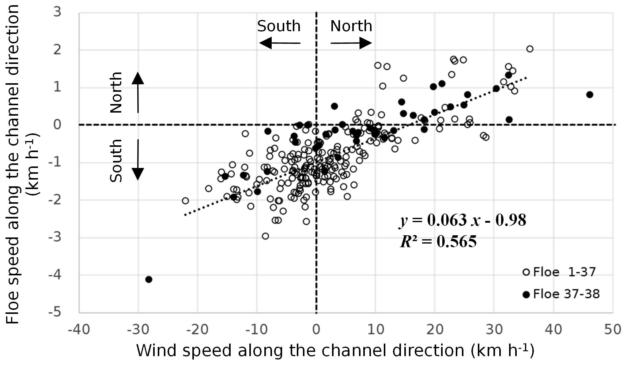
Figure 10Scatter plot of wind versus ice floe speed components along the Robeson Channel direction. Positive and negative values pertain to wind or ice motion heading north or south, respectively. Data from 39 floes drifting within the Robeson Channel are shown. The open circles pertain to 37 ice floes that originated north of the Robeson Channel and then formed part of the drifted ice regime in the Robeson Channel (where many ice floes existed). The closed circles represent data from two floes that originated inside the Robeson Channel and then drifted in the polynya formed after the ice arch was formed. The dashed line is the linear regression for the data of the 37 floes.
Table 3Results from the multivariate regression analysis showing the contributions of wind and ocean current to ice floe motion.
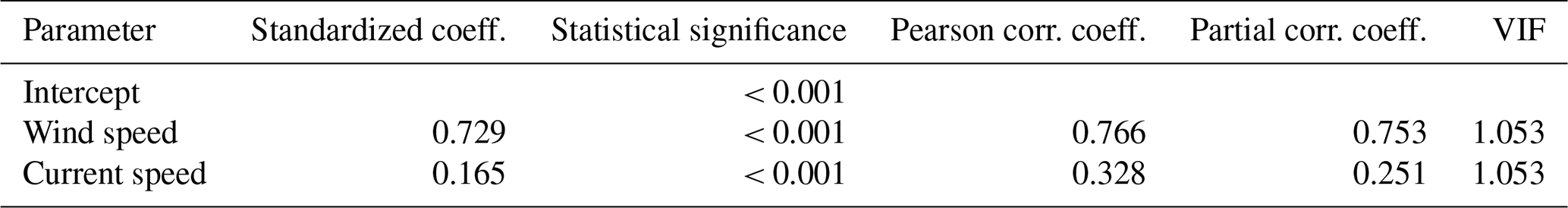
Isolating the wind and ocean current contributions to ice motion can be better achieved using a modelling approach, as presented in Thorndike and Colony (1982) and Kimura and Wakatsuchi (2000). However, in order to achieve this task using the present data of daily gridded wind and ocean current, we performed multivariate regression analysis, with the wind and current data as the independent variables and ice floe speed as the dependent variable. Only the components along the Robeson Channel extent were considered. The results are shown in Table 3. The standardized coefficient is a measure of how much an independent variable explains the dependent variable. In this case, the wind and current speed can explain 0.729 and 0.165 of the ice floe motion, respectively. Statistical significance is the probability of rejecting the null hypothesis, which is no significant difference between the contribution of wind and current, in this case. The Pearson correlation coefficient is a statistic that measures the linear correlation between two variables. Here, the wind shows a better linear correlation with the ice floe motion. The partial correlation coefficient is a measure of the correlation between the dependent variable and one independent variable, in the absence of other independent variables. Once again, the results show the more significant contribution of the wind. The variance inflation factor (VIF) should be < 10, otherwise there is severe multicollinearity in the model. The conclusion from these results is that wind speed has a greater influence on ice floe motion than ocean current in the open-drift (40 %–60 % ice concentration) or very-open-drift (< 40 % ice concentration) regimes in the Robeson Channel.
4.1.4 Case study 2: an ice floe moving in the drifted ice regime in the Robeson Channel
Figure 11 shows a sequence of daily Sentinel-1 images from 14 to 19 November, where many ice floes originating from the north of the Robeson Channel can be seen. The path of the ice floe marked with the asterisk (floe no. 29) is linked to the coincident wind vectors in Fig. 12. This ice floe moved southward at a speed of 27.0 km d−1 between 14 and 15 November. During this period, the wind speed was between 5 and 20 km h−1, with a wide range of directions, but the strongest wind blew from the south to the northeast (Fig. 12). Apparently, this drift was more influenced by the north–south current in this case (daily current maps are not shown). The momentum of the incoming ice floes from the north is a possible explanation for this southward motion. Between 15 and 16 November, relatively strong wind with a speed between 20 and 37 km h−1 blew from the south. However, the entire set of floes appear to have drifted eastward. Once again, the wind did not trigger this motion. SSH can be a possible cause because it has a gradient that matches the drift direction (Fig. 7). Between 16 and 18 November, the same strong wind, which approached 30 km h−1, continued to blow to the northeast (Fig. 12), and the entire set of floes responded by drifting in the same direction. Floe no. 29 reached its highest speed of 11.77 km d−1 on 17 November. Between 18 and 19 November, the wind diminished, but a group of ice floes appeared to swirl clockwise. The current continued to be southward, and there was 100 % local ice concentration around floe no. 29.
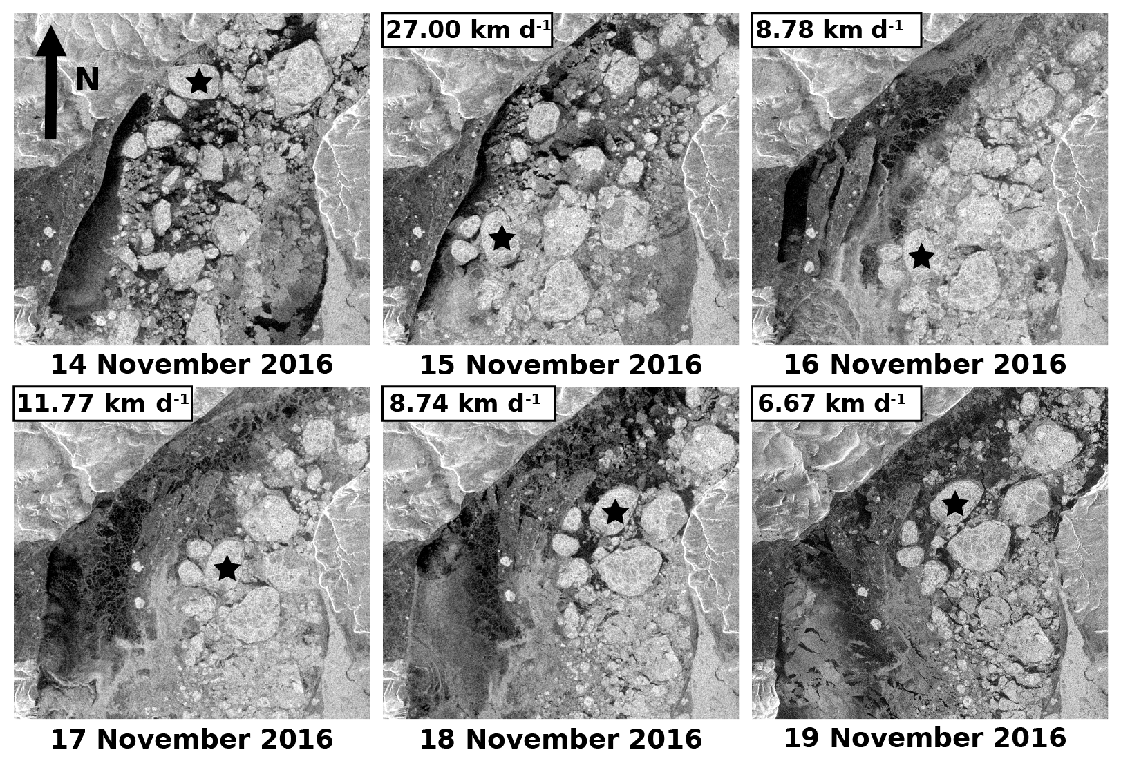
Figure 11A sequence of daily Sentinel-1 images showing the path of a number of ice floes. The floe marked by the asterisk (floe no. 29) is the subject of the comments in the text. Dates of the images are shown, as well as the speed of the marked floe.

Figure 12Maps of the 10 m level wind vectors (km h−1) from the ERA5 reanalysis. Each panel has vectors from the four grid points surrounding the location of ice floe no. 29 every 3 h during the time between the daily overpasses of Sentinel-1. For example, the 14–15 November panel has the 3 h vectors between the acquisition times of 14 and 15 November.
4.1.5 Case study 3: an ice floe drifting in the polynya within the Robeson Channel
Figure 13 shows the track of ice floe no. 38, which broke off from landfast ice at the Greenland side and drifted north and then south in the polynya regime. The trajectory covers the period from 8 to 22 February 2017, after the arch formed. The daily wind vector maps associated with the selected floe location are presented in Fig. 14. Between 10 and 11 February, northward wind dominated, although this never exceeded 20 km h−1. The ice floe drift of nearly 12 km d−1 matched the wind direction. Between 13 and 17 February, the northward wind accelerated, reaching 40 km h−1 and then 50 km h−1. The ice floe moved in the same direction, with its speed reaching 11.8, 32.2 and 20.4 km d−1 on 15, 16 and 17 February, respectively. The speed was significantly reduced to 3.7 km d−1 on 18 February as the floe approached the ice arch. After this day, the wind blew from the north and the ice floe changed its direction of motion to advancing southward. It is interesting to note the high ice floe speed of 43.0 km d−1 between 20 and 21 February and the highest speed of 99.1 km d−1 between 21 and 22 February. The latter was triggered by the highest wind encountered in this study, which gusted to 50 km h−1. However, it is important to recall that the surface current drives ice motion in the same direction. This case study demonstrates that the influence of the wind on ice motion is the greatest in areas of thin ice and water.

Figure 13Trajectory of an ice floe (floe no. 38) that separated from landfast ice and drifted in the polynya regime downstream of the ice arc. The track is shown from 8 to 22 February 2017.

Figure 14Maps of the 10 m level wind (km h−1), as shown in Fig. 12, but for ice floe no. 38, which was separated from landfast ice and drifted in the polynya downstream from the ice arch formed at the inlet of the Robeson Channel.
4.2 Formation of the ice arch
The ice arch phenomenon is a necessary condition for polynya formation downstream. Polynyas can be driven by wind action that removes newly formed ice (latent heat polynya) and/or warm upwelling ocean water that melts the ice as soon as it is forms (sensible heat polynya) (Smith et al., 1990). However, if the flux of ice from a nearby source continues to feed into the area that would become a polynya, then the polynya can only be formed if a natural obstacle develops to block the flux. This obstacle could be an ice arch, which is a mechanically strong formation that can withstand the massive dynamic load of the advected sea ice. Clearly, this factor is irrelevant to coastal polynyas as they are backed by land. This is more common in the Antarctic region (Nihashi and Ohshima, 2015). In the case of the Robeson Channel, an ice arch commonly forms at the inlet of the channel, blocking the ice flux from the Lincoln Sea into the Robeson Channel. The ice arch may collapse a few weeks after formation or persist as late as mid-August (Samelson et al., 2006). More historical context about the ice arches that form at the inlet of the Robeson Channel can be found in Kwok et al. (2010), Ryan and Münchow (2017), and Moore and McNeil (2018). The ice arch observed in the present dataset started its development on 24 January, matured on 1 February and collapsed in May 2017. The mechanism of arch development is described below. After its initial formation, chunks of ice continued to detach from the arch's contour under the action of the southward wind. This altered the arch's shape and the location of its terminal points along the two constriction points at the Greenland and Ellesmere Island sides. The sequence of the development is revealed in the set of Sentinel-1 images shown in Fig. 15.
The white dashed line that appears in some panels represents the arch's contour of the following day. For example, the dashed line in the image for 24 January represents the arch's contour that appears in the image for 25 January, and so on. No line is presented if the contour remained unchanged in the following day (e.g. the cases of 25 and 26 January). The difference between the visible arch and the dotted line in the image of any given day identifies the ice that was detached by the wind action on that day. The 3 h wind vectors during the period between the two daily overpasses of Sentinel-1, obtained from the ERA5 reanalysis, are presented in Fig. 16. Data were obtained from the grid points located on lines 3, 4 and 5 in Fig. 3 and are shown in the same colour as that figure.
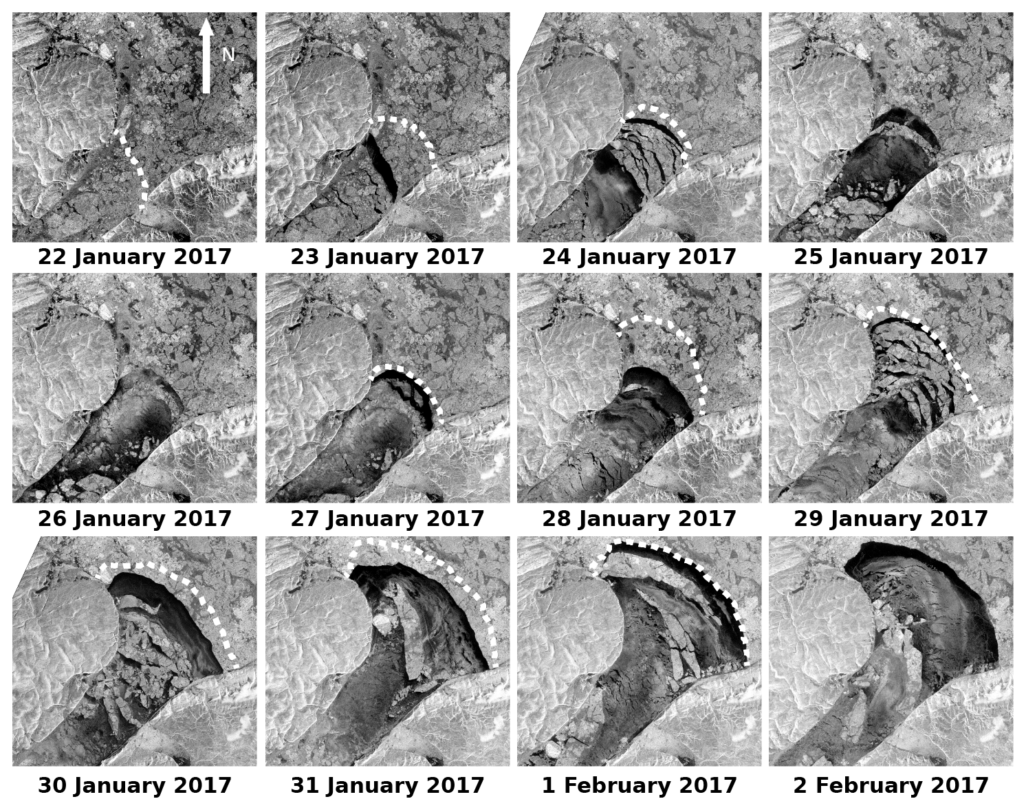
Figure 15Daily Sentinel-1 images showing the development of the arch formation from 24 January 2017 until it matured on 2 February 2017. The dotted line marks the arch shape and location in the following day.
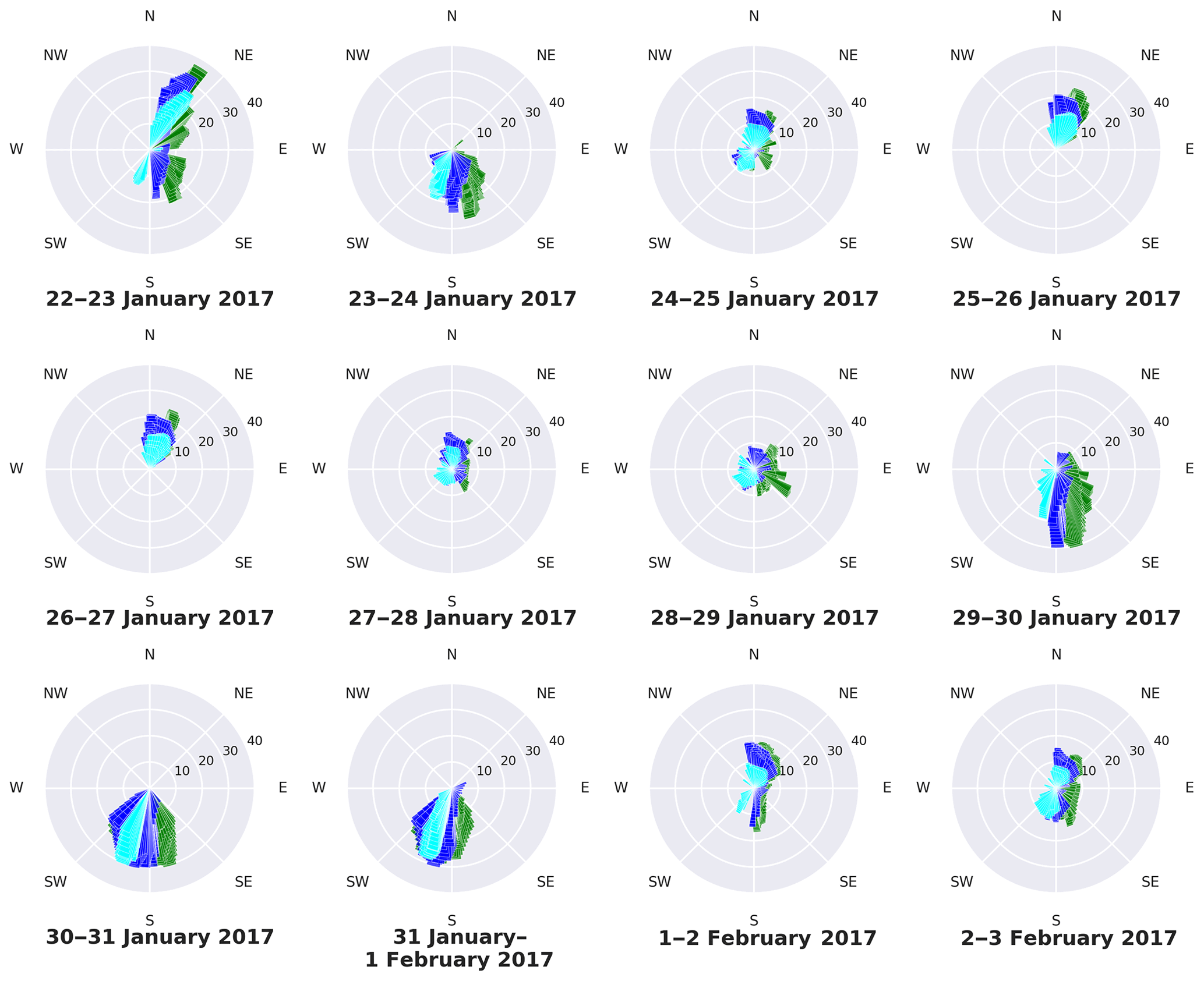
Figure 16Wind speed (km h−1) during the formation period of the ice arch (22 January to 3 February 2017), obtained from grid points on lines 3, 4 and 5 (corresponding to latitudes 82.5, 82.25 and 82∘ N, respectively) of the ERA5 reanalysis shown in Fig. 3. The colours of the vectors are the same as those of the grid points in Fig. 3.
After 7 d of persistent northward wind, southeastward wind returned for a few hours between 22 and 23 January. A wide rupture of ice cover, not forming an arch shape, can be observed in the 23 January image (Fig. 15). Between 23 and 24 January, the dominant southward wind (about 30 km h−1) was strong enough to cause many cracks in the ice cover and introduced the first visible contour of the arch on 24 January. On 25 January, the cracked ice drifted southward and another piece of ice was detached from the arch. On that day, light northward wind occurred (< 20 km h−1) but varied over the entire angular range. The same wind prevailed until 28 January, and no change in the arch was observed. When the strong southward wind, reaching 30 km h−1, prevailed from 29 January until 1 February, it first caused numerous cracks to appear on 29 January. The cracked ice was then pushed further south, leaving a well-defined arch shape, as can be seen in the image for 30 January. A major displacement of the arch's end point at the Ellesmere Island side (13.88 km) can be observed. The arch shape continued to be adjusted on 31 January and 1 February, in response to the same strong southward wind. Note the two large pieces of ice that detached in these 2 d (Fig. 15). After 1 February, the arch remained unchanged, regardless of the wind speed and direction, until it collapsed on 11 May. The only exception was the breakup of a large piece, defined as floe no. 39, on 5 March (Fig. 17). This piece broke off while the wind was dominantly northward (between 15 and 30 km h−1). This is not consistent with the aforementioned scenario of the modulation of the arch shape under the action of southward wind. However, it should be noted that the rest of the ice cover in the image for 5 March in Fig. 17 appears to shift north following the northward wind, as indicated by the arrow.
The arch legs, which is an engineering term that refers to the end parts of the arch, can be observed to be perpendicular to the land contour (see the images for 1 and 2 February in Fig. 15). As all the forces exerted on the arch's contour are transferred as compression forces, the arch legs must be perpendicular to the surface, in order to provide a robust way to transfer the load directly to the rock base at both sides. Otherwise, the end point of the arch may continue to slip at the surface, leading to eventual failure of the arch (Karnovsky, 2012). This feature, along with the curvature of the arch, will be of interest to the ice mechanics community.
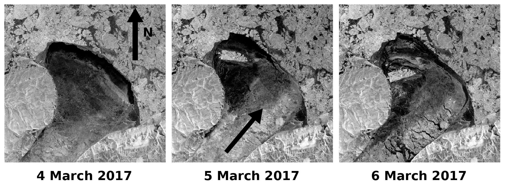
Figure 17Sequential Sentinel-1 images showing the breakup and drift of an ice piece that was labelled floe no. 39 in this study. This modulated the ice arch. The arrow indicates the dominant wind direction between the acquisition times of the images for 4 and 5 March.
The above discussion highlights the mechanism of ice arch formation. To reiterate, strong southward wind plays an important role in modulating the arch's contour as it may cause detachment of pieces of ice at the locations of fractures. Northward wind, on the other hand, has virtually no effect on the arch's shape and location. On two occasions, ice pieces were observed to detach in the presence of a light northward wind, which suggests the possible influence of the sea surface current. The modulation of the arch's shape abates when the upstream ice becomes too compacted to allow crack formation, and hence further detachment of ice pieces occurs in response to a southward wind. Moreover, the mechanically strong structure of the arch cannot fail under the dynamic force of the incoming ice flux. The structural properties of the arch were not addressed in this study, except for the observed configuration of its terminal points (arch legs) being perpendicular to the land surface.
In this study, a series of daily Sentinel-1A/1B images were used to study the sea ice motion at the scale of individual ice floes in the Robeson Channel, which is located between Greenland and Ellesmere Island, and the process of ice arch formation at the northern entry of the channel. The study period spanned the autumn and winter seasons of 2016/2017. Wind data from the ERA5 reanalysis were used to explore the role of wind on ice floe drift and the arch formation process. Daily gridded data of ocean current were also used. In total, 39 floes were visually tracked in the sequential daily images and their velocity vectors were calculated. Qualitative and statistical data of the ice drift were obtained in two regimes, upstream and within the Robeson Channel. Case studies showing links between the drift of selected ice floes and their driving forces were presented. The local reanalysis wind was obtained from the closest grid points to the ice floe at each location on its trajectory.
Sea ice that approaches the Robeson Channel follows a path around the northern section of Ellesmere Island. No ice drift was observed along the coast of Greenland in this case. In the convergent zone that leads to the channel, ice floes drift at a fairly constant speed of around 5 km d−1 along erratic paths. This motion seems to be mostly affected by the internal stresses between ice floes in such close pack ice (concentration > 70 %), with no influence of wind. Wind appears to influence the motion only if the floe is surrounded by thin ice or open water. In this case, a drift speed of up to 18 km d−1 was calculated.
Once an ice floe crosses the entry to the channel and becomes released from the stresses engendered by the surrounding ice, it starts to accelerate. While inside the channel, the ice floe drift speed varies between 15 and 45 km d−1. The direction of motion can be explained by the combination of wind and ocean currents. A single linear regression analysis between the wind and drift components along the extent of the channel revealed the increasing influence of the wind on ice floe motion when the surrounding ice cover features thin sheet and water. A multivariate regression analysis confirmed that the wind speed and ocean current speed can explain 72.9 % and 16.5 % of the ice floe speed, respectively. Available tidal data obtained from the deployed buoys prior to the study period were examined, but no conclusive impact of tide on ice floe motion was found from generating and examining the Fourier spectra of the data.
Ice arch formation and development were monitored using the daily Sentinel-1 images over a 9 d period from 24 January to 1 February 2017. During this period, pieces of ice along the arch's contour continued to crack and detached under the action of southward wind. Northward wind had no role in this process as it closed and tended to stabilize the arch. The process continued until the pack ice upstream of the arch became fully consolidated and the arch took on a mechanically strong concave shape.
The findings of this study will provide clues to enhance the dynamic modelling of ice by identifying conditions that accentuate the role of wind in ice motion. The study has also demonstrated the possibility of generating non-gridded drift vectors of individual sea ice floes by tracking their motion in a sequence of daily SAR images. Such a product would be important for operational ice mapping as it can identify the distribution of hazardous floes. Daily SAR images covering a limited number of geographic regions have become available from the Sentinel-1 system. They may soon be available from the recently launched RADARSAT Constellation Mission (RCM) (a fleet of three satellites) but only upon request. More SAR constellation systems are expected in the future from several national and commercial agencies. The challenge of generating maps of ice floe drift for sequential SAR images resides in developing an automated identification method for ice floe contours, considering their deformation, rotation, breakup and amalgamation while drifting.
Sentinel-1 data are available free of charge from the Copernicus Open Access Hub (European Space Agency, available at https://scihub.copernicus.eu/, last access: 27 October 2020). All the reanalysis data are publicly available. The ERA5 hourly data are available from https://cds.climate.copernicus.eu/cdsapp#!/dataset/reanalysis-era5-single-levels?tab=overview (C3S, 2017, last access: 27 October 2020), the ERA-Interim data are available from https://apps.ecmwf.int/datasets/data/interim-full-daily/levtype=sfc/ (Dee et al., 2011, last access: 27 October 2020), the NCEP/NCAR data are available from https://www.esrl.noaa.gov/psd/data/gridded/data.ncep.reanalysis.html (Kalnay et al., 1996, last access: 27 October 2020), the NCEP/DOE data are available from https://www.esrl.noaa.gov/psd/data/gridded/data.ncep.reanalysis2.html (Kanamitsu et al., 2002, last access: 27 October 2020), and the GLORYS12V1 data are available from http://marine.copernicus.eu/services-portfolio/access-to-products/?option=com_csw&view=details&product_id=GLOBAL_REANALYSIS_PHY_001_030 (last access: 12 December 2019). The Alert Station data can be obtained from https://climate.weather.gc.ca/historical_data/search_historic_data_e.html (Environment Canada, 2020, last access: 27 October 2020).
MES prepared the manuscript, designed the experiments and performed the data analysis. ZHW collected and processed the data. TTL contributed to the data analysis and supported the writing and editing.
The authors declare that they have no conflict of interest.
We are grateful to the following organizations for providing the data used in this study. The European Space Agency (ESA) provided the Copernicus Sentinel-1A/1B product. The ECMWF provided the ERA5 and ERA-Interim reanalysis products. NCEP, NCAR and DOE provided their respective reanalysis products. The CMEMS provided their GLORYS12V1 reanalysis product. The authors would also like to thank the two anonymous reviewers, whose comments have improved the manuscript greatly.
This work was supported in part by the National Key Research and Development Program of China (no. 2018YFC1406102), the fund of the Key Laboratory of Global Change and Marine-Atmospheric Chemistry (no. GCMAC1806), and the National Natural Science Foundation of China (nos. 41676179 and 41941010).
This paper was edited by Yevgeny Aksenov and reviewed by two anonymous referees.
Bourbigot, M., Johnsen, H., Piantanida, R., and Hajduch, G.: Sentinel-1 product definition, MDA, SEN-RS-52-7440, 2016.
Copernicus Climate Change Service (C3S): ERA5: Fifth generation of ECMWF atmospheric reanalyses of the global climate, Copernicus Climate Change Service Climate Data Store (CDS), https://doi.org/10.24381/cds.adbb2d47, 2017.
Dee, D. P., Uppala, S. M., Simmons, A. J., Berrisford, P., Poli, P., Kobayashi, S., Andrae, U., Balmaseda, M. A., Balsamo, G., Bauer, P., Bechtold, P., Beljaars, A. C. M., van de Berg, I., Biblot, J., Bormann, N., Delsol, C., Dragani, R., Fuentes, M., Greer, A. J., Haimberger, L., Healy, S. B., Hersbach, H., Holm, E. V., Isaksen, L., Kallberg, P., Kohler, M., Matricardi, M., McNally, A. P., Mong-Sanz, B. M., Morcette, J.-J., Park, B.-K., Peubey, C., de Rosnay, P., Tavolato, C., Thepaut, J. N., and Vitart, F.: The ERA-Interim reanalysis: Configuration and performance of the data assimilation system, Q. J. Roy. Meteorol. Soc., 137, 553–597, https://doi.org/10.1002/qj.828, 2011.
Demchev, D., Volkov, V., Kazakov, E., Alcantarilla, P. F., Sandven, S., and Khmeleva, V.: Sea ice drift tracking from Sequential SAR images using accelerated-KAZE features, IEEE T. Geosci. Remote, 55, 5174–5184, https://doi.org/10.1109/TGRS.2017.2703084, 2017.
Dumont, D., Gratton, Y., and Arbetter, T. E.: Modelling the dynamics of the North Water Polynya ice bridge, J. Phys. Oceanogr., 39, 1448–1461, https://doi.org/10.1175/2008JPO3965.1, 2009.
Environment Canada: Historical Hourly Data, available at: https://climate.weather.gc.ca/historical_data/search_historic_data_e.html, last access: 27 October 2020.
European Space Agency (ESA): Copernicus Open Access Hub, available at: https://scihub.copernicus.eu/, last access: 27 October 2020.
Fernandez, E. and Lellouche, J. M.: Product user manual for the Global Ocean Physical Reanalysis Product GLORYS12V1, Copernicus Product User Manual, 4, 1–15, 2018.
Gimbert, F., Marsan, D., Weiss, J., Jourdain, N. C., and Barnier, B.: Sea ice inertial oscillations in the Arctic Basin, The Cryosphere, 6, 1187–1201, https://doi.org/10.5194/tc-6-1187-2012, 2012.
Godin, G.: Currents in Robeson Channel, Nares Strait, Mar. Geod., 2, 351–364, https://doi.org/10.1080/15210607909379362, 1979.
Gudmandsen, P.: A remote sensing study of Lincoln Sea, in: Proceeding of the ERS-ENVISAT Symposium, Gothenburg, Sweden, 16–20 October, 461, 2084–2090, 2000.
Hall, R. T. and Rothrock, D. A.: Sea ice displacement from Seasat Synthetic Aperture Radar, J. Geophys. Res.-Ocean, 86, 1078–1082, https://doi.org/10.1029/JC086iC11p11078, 1981.
Herlinveaux, R. H.: Oceanographic observations in Robeson Channel, N.W.T., Pacific Marine Science Report 79–16, Institute of Ocean Science, Patricia Bay, Sidney, BC, Canada, 1971.
Johnson, H. L., Münchow, A., Falkner, K. K., and Melling, H.: Ocean circulation and properties in Petermann Fjord, Greenland, J. Geophys. Res., 116, C01003, https://doi.org/10.1029/2010JC006519, 2011.
Kalnay, E., Kanamitsu, M., Kistler, R., Collins, W., Deaven, D., Gandin, L., Iredell, M., Saha, S., White, G., Woollen, J., Zhu, Y., Chelliah, M., Ebisuzaki, W., Higgins, W., Janowiak, J., Mo K. C., Ropelewski, C., Wang, J., Leetmaa, A., Reynolds, R., Jenne, R., and Dennis, J.: The NCEP/NCAR 40-year reanalysis project, B. Am. Meteor. Soc., 77, 437–470, https://doi.org/10.1175/1520-0477(1996)077<0437:TNYRP>2.0.CO;2, 1996.
Kanamitsu, M., Ebisuzaki, W., Woollen, J., Yang, S.-K., Hnilo, J. J., Fiorino, M., and Potter, G. L.: NCEP-DOE AMIP-II Reanalysis (R-2), B. Am. Meteor. Soc., 83, 1631–1644, https://doi.org/10.1175/bams-83-11-1631, 2002.
Karnovsky, I. A.: Theory of arched structures: strength, stability and vibration, Springer, New York Dordrecht Heidelberg London, 423 pp., https://doi.org/10.1007/978-1-4614-0469-9, 2012.
Kimura, N. and Wakatsuchi, M.: Relationship between sea-ice motion and geostrophic wind in the Northern Hemisphere, Geophys. Res. Lett., 27, 3735–3738, https://doi.org/10.1029/2000GL011495, 2000.
Kwok, R.: Variability of Nares Strait ice flux, Geophys. Res. Lett., 32, L24502, https://doi.org/10.1029/2005GL024768, 2005.
Kwok, R. and Cunningham, G. F.: Seasonal ice area and volume production of the Arctic Ocean: November 1996 through April 1997, J. Geophys. Res.-Ocean, 107 (C10), 8038, https://doi.org/10.1029/2000JC000469, 2002.
Kwok, R., Spreen, G., and Pang, S.: Arctic sea ice circulation and drift speed: Decadal trends and ocean currents, J. Geophys. Res.-Oceans, 118, 2408–2425, https://https://doi.org/10.1002/jgrc.20191, 2013.
Kwok, R., Toudal-Pederson, L., Gudmandsen, P., and Pang, S.: Large sea ice outflow into Nares Strait in 2007, Geophys. Res. Lett., 37, L03502, https://doi.org/10.1029/2009GL041872, 2010.
Leberl, F., Raggam, J., Elachi, C., and Campbell, W. J.: Sea ice motion measurements from SEASAT SAR images, J. Geophys. Res.-Ocean, 88, 1915–1928, https://doi.org/10.1029/JC088iC03p01915, 1983.
Lellouche, J.-M., Greiner, E., Le Galloudec, O., Garric, G., Regnier, C., Drevillon, M., Benkiran, M., Testut, C.-E., Bourdalle-Badie, R., Gasparin, F., Hernandez, O., Levier, B., Drillet, Y., Remy, E., and Le Traon, P.-Y.: Recent updates to the Copernicus Marine Service global ocean monitoring and forecasting real-time 1∕12∘ high-resolution system, Ocean Sci., 14, 1093–1126, https://doi.org/10.5194/os-14-1093-2018, 2018.
Leppäranta, M.: The drift of sea ice, Springer Science & Business Media, https://doi.org/10.1007/978-3-642-04683-4, 2011.
McNutt, S. L. and Overland, J. E.: Spatial hierarchy in Arctic sea ice dynamics, Tellus A, 55, 181–191, https://doi.org/10.1034/j.1600-0870.2003.00012.x, 2003.
Moore, G. W. K and McNeil, K.: The early collapse of the 2017 Lincoln Sea ice arch in response to atmospheric sea ice and wind forcing, Geophys. Res. Lett., 45, 8343–8351, https://doi.org/10.1029/2018GL078428, 2018.
Münchow, A. and Melling, H.: Ocean current observations from Nares Strait to the west of Greenland: Interannual to tidal variability and forcing, J. Mar. Res., 66, 801–833, https://doi.org/10.1357/002224008788064612, 2008.
Münchow, A., Falkner, K. K., and Melling, H.: Spatial continuity of measured seawater and tracer fluxes through Nares Strait, a dynamically wide channel bordering the Canadian Archipelago, J. Mar. Res., 65, 759–788, https://doi.org/10.1357/002224007784219048, 2007.
Nihashi, S. and Ohshima, K. I.: Circumpolar map of Antarctica coastal polynya and landfast sea ice: relationship and variability, J. Climate, 28, 3650–3670, https://doi.org/10.1175/JCLI-D-14-00369.1, 2015.
Ryan P. A. and Münchow, A.: Sea ice draft observations in Nares Strait from 2003 to 2012, J. Geophys. Res.-Oceans, 122, 3057–3080, https://doi.org/10.1002/2016JC011966, 2017.
Rasmussen, T. A. S., Kliem, N., and Kaas, E.: Modelling the sea ice in the Nares Strait, Ocean Model., 35, 161–172, https://doi.org/10.1016/j.ocemod.2010.07.003, 2010.
Samelson, R. M., Agnew, T., Melling, H., and Münchow, A.: Evidence of atmospheric control of sea-ice motion through Nares Strait, Geophys. Res. Lett., 33, L02506, https://doi.org/10.1029/2005GL025016, 2006.
Shroyer, E. L., Samelson, R. M., Padman, L., and Munchow, A.: Modeled ocean circulation in Nares Strait and its dependence on landfast-ice cover, J. Geophys. Res.-Oceans, 120, 7934–7959, https://doi.org/10.1002/2015JC011091, 2015.
Smith, S. D., Muench, R. D., and Pease, C. H.: Polynyas and leads: An overview of physical processes and environment, J. Geophys. Res.-Oceans, 95), 9461–9479, https://doi.org/10.1029/JC095iC06p09461, 1990.
Tang, C. L., Ross, C. K., Yao, T., Petrie, B., DeTracey, B. M., and Dunlap, E.: The circulation, water masses and sea-ice of Baffin Bay, Prog. Oceanogr., 63, 183–228, https://doi.org/10.1016/j.pocean.2004.09.005, 2004.
Thorndike, A. S. and Colony, R.: Sea ice motion in response to geostrophic winds, J. Geophys. Res.-Ocean, 87, 5845–5852, https://doi.org/10.1029/JC087iC08p05845, 1982.
Vincent, R. F., Mardsen, R. F., and McDonald, A.: Short time-span ice tracking using sequential AVHRR imagery, Atmos.-Ocean, 39, 279–288, https://doi.org/10.1080/07055900.2001.9649681, 2001.
Wekerle, C., Wang, Q., Danilov, S., Jung, T., and Schröter, J.: The Canadian Arctic Archipelago throughflow in a multiresolution global model: Model assessment and the driving mechanism of interannual variability, J. Geophys. Res.-Oceans, 118, 4525–4541, https://doi.org/10.1002/jgrc.20330, 2013.