Observation-derived ice growth curves show patterns and trends in maximum ice thickness and safe travel duration of Alaskan lakes and rivers

The formation, growth, and decay of freshwater ice on lakes and rivers are fundamental processes of northern regions with wide-ranging implications for socio-ecological systems. Ice thickness at the end of winter is perhaps the best integration of cold-season weather and climate, while the duration of thick and growing ice cover is a useful indicator for the winter travel and recreation season. Both maximum ice thickness (MIT) and ice travel duration (ITD) can be estimated from temperature-driven ice growth curves fit to ice thickness observations. We simulated and analyzed ice growth curves based on ice thickness data collected from a range of observation programs throughout Alaska spanning the past 20–60 years to understand patterns and trends in lake and river ice. Results suggest reductions in MIT (thinning) in several northern, interior, and coastal regions of Alaska and overall greater interannual variability in rivers compared to lakes. Interior regions generally showed less variability in MIT and even slightly increasing trends in at least one river site. Average ITD ranged from 214 d in the northernmost lakes to 114 d across southernmost lakes, with significant decreases in duration for half of sites. River ITD showed low regional variability but high interannual variability, underscoring the challenges with predicting seasonally consistent river travel. Standardization and analysis of these ice observation data provide a comprehensive summary for understanding changes in winter climate and its impact on freshwater ice services.

1 Introduction

Arctic amplification is an enhanced warming response in high latitudes relative to increasing global temperature (Serreze and Barry, 2011). Though not yet completely understood, sea ice decline and associated climate feedbacks are considered to be major drivers of this process (Serreze and Francis, 2006). A salient feature of arctic amplification is greater warming during winter, which has been strikingly apparent in Alaska during recent years (Wendler et al., 2014; Walsh and Brettschneider, 2019). Terrestrial landscape responses to winter climate change are perhaps most quantifiable in ice formation and growth on lakes and rivers, as well as readily described by ice thickening through the winter (Allen, 1977; Engram et al., 2018). Freshwater ice thickness and duration may function as robust integrators of winter climate, as they respond both to changes in air temperature and snow accumulation. Additionally, ice thickness and its duration have important implications for winter travel, subsistence, and recreation in Alaska and across the Arctic (Brown and Duguay, 2010; Schneider et al., 2013; Cold et al., 2020).

Some of the longest ice thickness records come from the Barrow Peninsula in northernmost Alaska, where lake ice historically grew greater than 2 m thick in some years by winter's end as recorded in the 1970s (Weeks et al., 1978) and 1990s (Zhang and Jeffries, 2000). In recent years, however, MIT did not exceed 1.2 m in snowy winters, when ice was well insulated and air temperatures were unusually warm (Arp et al., 2018). The impacts of arctic amplification on freshwater ice should be most evident in this northern coastal region where Alexeev et al. (2016) demonstrated a linkage between sea ice extent and lake ice growth. This long, yet intermittent, record of lake ice thickness in northern Alaska comes from a variety of observation efforts including community-based monitoring facilitated by government agencies (Bilello, 1980) and school science programs (Morris and Jeffries, 2010). These same community-based monitoring programs also contributed to shorter, but still highly valuable, ice thickness records for other lakes and rivers in Alaska, which have been maintained and extended by the National Weather Service's Alaska-Pacific River Forecast Center (APRFC). APRFC's interest in ice thickness has primarily been to facilitate river breakup and ice jam forecasting but is also of value for informing safe ice travel, as fall through accidents have increased in recent years (Fleischer et al., 2014).

In contrast to ice thickness observations, records and analyses of ice phenology (timing of freeze-up and breakup) are often long and abundant for many northern regions, likely owing to the ease of observing water-to-ice transition timing from shorelines, aircraft, or satellites (Brown and Duguay, 2010). Rigorous satellite-based observations show distinct trends towards earlier breakup on both rivers (Cooley and Palvesky, 2016) and lakes (Smejkalova et al., 2017) in Alaska, and longer-term observer records from other northern regions show similar patterns (e.g., Magnuson et al., 2000; Weyhenmeyer et al., 2011). Detection of trends in freeze-up timing is often less certain (Brown and Duguay, 2010), though recent analyses suggest late freeze-up contributions to reduced ice cover duration on lakes (Sharma et al., 2019) and rivers (Yang et al., 2020). Brown et al. (2018) tracked both freeze-up and breakup progression in Alaskan rivers, highlighting the varying stages of ice formation and decay processes relative to access for over ice travel, and this suggests the need to move beyond ice phenology as an exact to-the-day event. Tracking changes in ice thickness through the winter cold season provide the simplest means of quantifying this continuum, though these data are distinctly more field intensive.

Reported analyses of ice thickness datasets often lack detection of thinning trends despite progressive winter warming, which may be due to high interannual variability in snowfall and the dominant role of snow insulation on ice growth (Brown and Duguay, 2010). Yet the majority of studies analyzing ice thickness trends that we are aware came before unprecedented warm winters during the last decade in Alaska (Wendler et al., 2014; Walsh and Brettschneider, 2019). We also suspect that the inherent nature of ice thickness data collection, in which the timing of late winter measurement may vary from year to year relative to slight shifts in the ice growth season, adds additional noise in detecting trends. Other factors related to ice observations include that ice thickness can vary significantly within a small area depending on snow cover, measurement protocols have often differed among programs, and rural community observers are often volunteers with high turnover and minimal oversight. Large data gaps in records also make it difficult to ascertain trends at some long-term sites (Cherry, 2019). For these reasons, we are motivated to standardize ice thickness according to ice growth curves informed by field observations and calculate relevant metrics, maximum ice thickness (MIT) and ice travel duration (ITD), as well as to merge analyses of both river and lake ice in Alaska.

In this study, we organized winter lake and river ice thickness observations from a variety of sources to provide an updated analysis of patterns and trends of ice growth in Alaska from 1962 to present. Fitting these data to air-temperature-driven ice growth curves simulated with the Stefan equation (Stefan, 1891; Jumikis, 1977) provides a robust seasonal estimation of changing ice thickness for multiple sites with proximate climate data. The ice growth curves were used to estimate MIT and ITD for four lakes and four rivers distributed across Alaska, with records spanning 20 years or greater, to provide a summary of recent changes in ice of climatic and societal relevance. Several shorter records are also presented for spatial comparison.

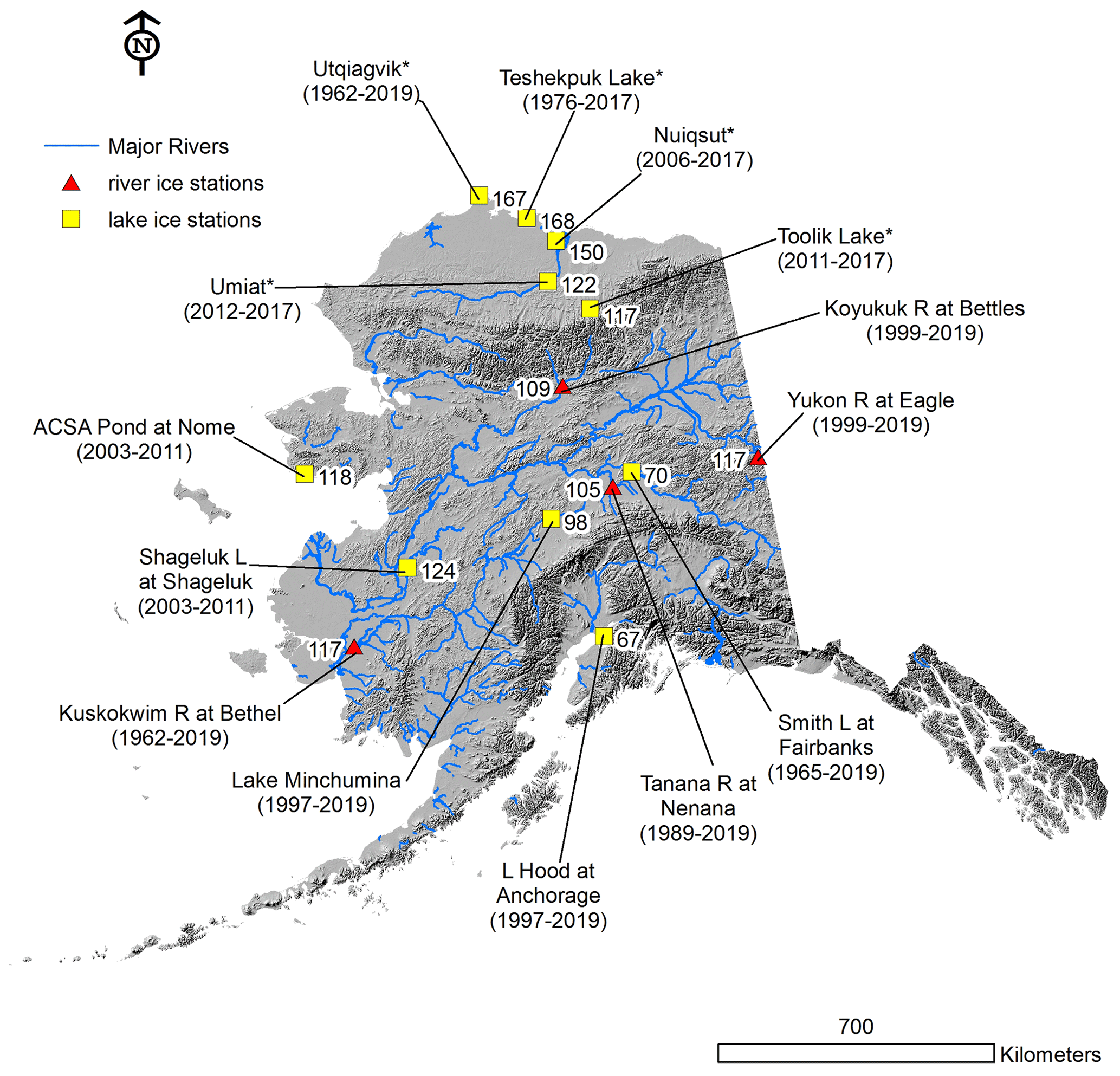
Figure 1 Map of the State of Alaska with all observation locations by water body and nearest community indicated as well as average maximum ice thickness (cm) for each period of record (in parenthesis). Several shorter-term records (<20 years) which are not presented in the main analysis are shown here for additional context (* indicates that observations are based on multiple lakes or rivers within a region; 300 m digital elevation model hillshade is USGS data in the US public domain).

2 Background and methods

2.1 Study region and water bodies

The diverse geographic and northern climatic setting of the State of Alaska presents a fascinating study region to observe freshwater ice (Arp and Jones, 2009; Arp et al., 2013). Even though the State of Alaska is a geopolitical unit, its vast size (1.5 million km²), expansive latitudinal extent (18^∘), wide longitudinal extent (58^∘), lengthy coastline (54 500 km), and complex tectonic setting create a largely contiguous landscape with several large mountain ranges and expansive river valleys (Fig. 1). These geographical attributes of Alaska interact with climate, glacial history, and soil conditions (particularly permafrost) to create many lakes (>400 000) and extensive and varied river networks (>150 000 km) (Arp and Jones, 2009). In contrast to water body extents, the Alaska road network is relatively short (<25 000 km) and not connected to the majority of towns and villages, which limits opportunities to maintain long-term observations of most water bodies. Thus the majority of sites with long-term ice observation data are associated with large towns along roadways or villages adjacent to rivers or lakes (Table 1). Another restriction for this study was proximity to reliable long-term air temperature data from weather stations, which are typically associated with larger airports.

Table 1 Summary of major ice observation stations and corresponding ice thickness records. Ice growth curves simulated using the Stefan equation and the average α coefficient (cm ^∘C${}^{-\mathrm{1}/\mathrm{2}}$ d${}^{-\mathrm{1}/\mathrm{2}}$) and accumulated freezing degree days (AFDD) at MIT (^∘C d) are reported for each station. Air temperature data from National Weather Service stations are indicated by station codes.

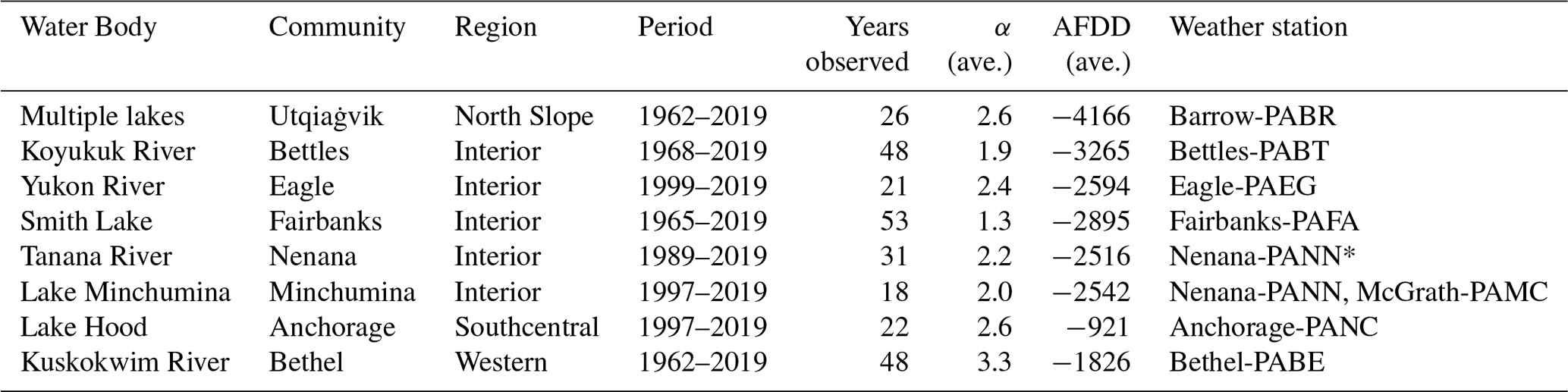
* Missing data derived from relationship to Fairbanks-PAFA.

2.2 Alaska ice observation programs

Scientific records of ice thickness measurements in Alaska date back to the First International Polar Year in 1882–1883 for lakes located near Barrow (Ray, 1885). Starting in the early 1960s the US Army Corps of Engineers Cold Regions Research and Engineering Laboratory (CRREL) established ice-observing stations in coordination with Canadian and US government agencies (Bilello, 1980). Stations included 26 lakes and rivers in Alaska where ice thickness data were collected at weekly intervals until at least 1974. Observations made by local residents (Alaska Natives, homesteaders, lodge keepers, teachers, and clergy) for up to 15 years, in some cases, provided valuable data for developing ice growth and decay models as reported in Bilello (1980) and other CRREL reports. Perhaps as importantly, these data provide a comprehensive summary of ice thickness and its variability over the climatically diverse region of the Arctic and sub-Arctic before notable climate warming. The majority of Alaska ice thickness data, as well as snow depth data, from this program are now archived with the Arctic Data Center (ADC) (Bilello, 2019). Observation protocols are not always well described in the reports for this program but likely relied on narrow gauge hand augers and tapes similar to current procedures, and the ice thickness observations per date may have come from single-point measurements.

A more recent winter observation program, Alaska Lake Ice and Snow Observatory Network (ALISON), pioneered the integration of science education with snow and ice physics in Alaska schools from 1999 to 2010 (Morris and Jeffries, 2010). While learning about snow and ice physics, students and teachers collected valuable datasets across a wide range of geographic and climatic settings, including at least 17 lakes ranging from the Barrow Peninsula in the north to the Kenai Peninsula in the south. Several of these sites overlap with CRREL stations, thus providing an opportunity for extension of records and temporal comparisons. ALISON's focus on snow depth, density, and heat flux provided additional data of value for understanding variability and modeling ice growth (Gould and Jeffries, 2005; Jeffries et al., 2005). ALISON datasets are also archived at ADC (Morris and Jeffries, 2019). Often up to 20 snow measurements were recorded per sampling interval for this program, while ice thickness was typically recorded from a single point using a thermal resistance (heated) wire known as a TWITT (Thermal Wire Ice Thickness Thingy; Martin Jeffries, personal communication, 2018). The TWITT was designed to minimize local snow disturbance that would affect subsequent measurements but also represents a single-point measurement of ice thickness.

An important Alaska ice record focused on breakup timing of a single river reach is the Nenana Ice Classic (NIC), where a tripod is set on the Tanana River by the community of Nenana each year and cabled to a clock to record the exact data of river breakup (Sagarin and Micheli, 2001). This community-based monitoring program dates back to 1917, and each year thousands of people submit breakup guesses into a pool, with the closest participants taking home > USD 300 000 in recent years. Regular ice thickness observations, dating back to at least 1989, have been made by community members who run the NIC and are published to provide contestants with additional information to aid in guesses.

A fourth and also contemporary Alaska-wide lake and river data source is provided by the National Weather Service (NWS) Alaska-Pacific River Forecast Center (APRFC). Prior to the establishment of the APRFC, the National Weather Service's weather forecast offices collected or solicited these data and maintained them at what is now the National Center for Environmental Information. Historic monthly ice thickness measurements have been compiled from a variety of sources including the CRREL dataset (Bilello, 1980), and contemporary observations come from NWS scientists and paid and volunteer observers in remote communities throughout the state. Much of this ice thickness data for both rivers and lakes are used in operational forecasting of river conditions specific to river breakup and ice jam flooding predictions. APRFC ice thickness data are available online (https://www.weather.gov/aprfc/IceThickness, last access: 1 December 2019). The current protocol for APRFC is to collect single-auger hole and tape observations near the start of the month from November to March near the same location at each water body below undisturbed snow.

Lastly, a regional lake ice observation program focused on Alaska's North Slope began in 2012 called the Circumarctic Lakes Observation Network (CALON) (Hinkel et al., 2012). This project supported by the National Science Foundation collected consistent late winter ice thickness data from sets of six lakes in each of 10 study areas arrayed from the Brooks Range foothills to the Beaufort Sea coastal plain until 2017. Several of these study areas were associated with field camps or other long-term research locations where prior lake ice data existed or were expected to continue after CALON concluded. Observations were made at the same location on each lake every year by drilling three to five holes at regular spacing and recording snow data in association with individual ice thickness measurements. ADC has CALON datasets archived for ice thickness (Arp, 2018a) and snow characteristics (Arp, 2018b) separately.

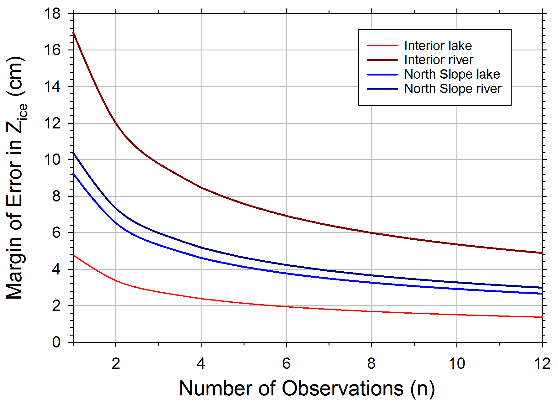
Figure 2 Margin of error analysis for Interior and North Slope lakes and rivers from samples of 36 evenly spaced measurements during the winter of 2018–2019.

Addressing the issue of data comparability among programs is relevant to this study. It is of course expected that higher numbers of samples per site correspond to more accurate ice thickness measurements such that CALON protocols have higher accuracy than some of the other ice observation programs described. Analysis conducted in a 36-member sampling protocol on two lakes and two rivers (one each in the Interior and the North Slope) showed that more samples reduced error (Fig. 2). This analysis suggests that making one observation (n=1) results in potential error up to 18, 10, 8, and 4 cm from the mean for Interior rivers, North Slope rivers, North Slope lakes, and Interior lakes, respectively. Three observations (n=3) results in potential error up to 9, 6, 5, and 3 cm from the mean for Interior rivers, North Slope rivers, North Slope lakes, and Interior lakes, respectively. While this analysis provides guidance for comparing the quality of differing ice observation approaches, we also suggest that professional experience or local knowledge in selecting locations of representative ice thickness may well overcome low sample size in many cases. Our expectation is that observers reporting to APRFC have such experience, as do observers from previous programs.

2.3 Ice growth curve simulation

For all records with late winter ice observations, we estimated MIT using the Stefan ice growth model (modified Stefan equation) (Eq. 1):

$$\begin{array}{}\text{(1)}& Z_{\mathrm{ice}}=\mathit{\alpha }\sqrt{\text{AFDD}},\end{array}$$

where α is the ice growth (thermal insulation or heat exchange) coefficient in cm ^∘C${}^{-\mathrm{1}/\mathrm{2}}$ d${}^{-\mathrm{1}/\mathrm{2}}$, and AFDD is accumulated freezing degree days in ^∘C d used to estimate ice thickness (Z_ice) in centimeters on a daily time step (Stefan, 1891; Jumikis, 1977). Mean daily air temperature data used to force this model were acquired from the nearest NWS station, the majority of which were within 20 km of the water body where ice was monitored (Table 1). In the cases of Shageluk and Lake Minchumina (Fig. 1), no adjacent NWS or other meteorological station air temperature records were available, and we averaged the records between two nearest stations set in opposing directions. Summation of AFDD was started at the date of estimated ice growth initiation each winter. When early ice thickness observations (i.e., Z_ice<10 cm) were available or actual observation of the day of ice initiation, these data guided selecting this date. When these data were not available, the more common case, we selected the date according to 3 consecutive days with mean daily temperature <0 ^∘C for lakes, which is based on previous camera and sensor observations (Arp et al., 2013) and 6 consecutive days <0 ^∘C for rivers. The later criteria for rivers are based on information from APRFC observers but are more limited and thus considered much more uncertain and a potential source of error in ice growth modeling on rivers. Both air temperature criteria follow guidance in Bilell (1964) and Ashton (1989) on ice cover initiation and early growth. Complementing the ice growth model (Eq. 1), is an ice decay model developed by Bilello (1980) (Eq. 2):

$$\begin{array}{}\text{(2)}& Z_{\mathrm{ice}}={\mathit{\alpha }}^{\prime }\text{ATDD},\end{array}$$

where α^′ is the ice decay coefficient in cm ^∘C⁻¹ d⁻¹ and ATDD is accumulated thawing degree days in ^∘C d, with 0 ^∘C and also with summation beginning at the day of ice growth initiation. Equation (2) is calculated concurrently with Eq. (1) to estimate the ice growth–decay curve (Fig. 3) for the winter season in lakes and rivers. The ice thickness curve was then fit to late winter Z_ice observations for winter season primarily by adjusting α. In some cases when observation came after the maximum in ATDD, α^′ was also adjusted to provide the best fit; otherwise α^′ was left constant (typically set at 1.0) among simulations with no effect on estimations of MIT or ITD. MIT was then extracted from each record as shown in the example ice growth curve in Fig. 3. All subsequent data analyses use the MIT as a standardized estimate of winter ice growth for each winter season and water body. Individual year estimates of MIT and the original ice thickness observations and corresponding model parameters will be archived and available at the ADC (Arp and Cherry, 2020).

Figure 3 Example ice growth and decay curves from Barrow lakes in a thick (a) and thin (b) ice year showing curve fits to observed data, the time when maximum ice thickness (MIT) is reached, and the period representing ice travel duration (ITD).

A new metric was also derived from each ice growth curve, which we term ice travel duration (ITD) or safe travel duration, and is intended to represent the period of time when most modes of common travel are safe according to ice thickness and continued thickening. Quantitatively this is defined as the date when ice thickness surpasses 30 cm to the date of MIT, the latter of which typically corresponds to the maximum AFDD and the start of ice decay (Fig. 3). Our rationale is that 30 cm exceeds the thickness when most vehicle travel is safe on freshwater ice. After MIT is reached and ice decay begins, even though its thickness typically well exceed 30 cm, its structural integrity and strength is changing rapidly such that thickness is less relevant to its load-bearing capacity (Gold, 1971; Leppäranta, 2015). In practice it is common for safe foot and snow machine travel on thicknesses less than 30 cm, and similar travel is common over thick ice that is starting to degrade. We also note that modeling ice growth during the initial thickening phase is less predictable by air temperature (Ashton, 1989) and thus selected a level of thickness where we expect this relationship to be more robust. To evaluate how closely this ITD start date tracked ice conditions identified by local APRFC observers, we compared “Safe for Vehicle” dates on three rivers and one lake common to our dataset when “snowmachine” was indicated for “Type of Vehicle” in the APRFC database (https://www.weather.gov/aprfc/freezeUp, last access: 1 February 2020) (Fig. 4a). This comparison showed a close match with an average offset ranging from +4 d on the Yukon River at Eagle to −5 d on Lake Minchumina. A similar comparison was made with the ITD end date tracked observer data (https://www.weather.gov/aprfc/breakupDB, last access: 1 February 2020) (Fig. 4b). For this comparison in all but two cases observer indications of “Safe for Vehicle” were always later than the date of maximum ice thickness, as we would have anticipated because it is common for travelers to use degrading ice safely for some period before complete breakup. Thus, our estimates of ITD should be considered conservative and for many modes of travel (and corresponding levels of caution) our estimates of ITD are shorter in duration that what is practiced locally.

Figure 4 Comparison of ice travel duration metric start (a) and end (b) dates for four study rivers and lakes to ice condition designations reported by Alaska-Pacific River Forecast Center (APRFC) observers.

2.4 Data analysis

Patterns and trends in MIT and ITD records for each station were primarily analyzed graphically in time series by comparison among lake and river sites. Detection of trends was done using linear regression for the entire record available for each water body. To separate or break MIT records into distinct periods of potential interest, we used a combination of piecewise linear regression to identify significant changes in trends and regime shift detection methods (Rodionov, 2004) to identify significant changes in means and variance. Gaps in observational data also resulted in gaps in MIT estimates, such that many of the breaks or record separations graphically selected correspond to these missing years of record. We report significant trends (p<0.05) and the means and standard deviations of MIT and ITD for all periods within the record, and this served as our primary basis for comparison and analysis. Multiple regression analysis was used to evaluate relationships between MIT and ITD to air temperature and upland snow depth data from proximate weather stations when available to evaluate general controls on interannual variability.

To understand the relative contributions of thermal forcing (air temperature) and thermal resistance (primarily snow insulation), we isolated these components from the Stefan equation (Eq. 1) over each MIT record per water body using power law analysis. In this approach thermal forcing is represented by AFDD (Eq. 3),

$$\begin{array}{}\text{(3)}& \sqrt{\text{AFDD}}=a{\text{MIT}}^b,\end{array}$$

and thermal resistance is represented by α (Eq. 4),

$$\begin{array}{}\text{(4)}& \mathit{\alpha }=c{\text{MIT}}^d,\end{array}$$

where the coefficients b and d represent the proportions of interannual variation in MIT explained by the AFDD and α, respectively, and should sum to 1 ($b+d=\mathrm{1}$). The additional check that this partitioning of variability follows a power law is that the product of the coefficients a and c are 1 ($a\times c=\mathrm{1}$). This approach is borrowed from hydraulic geometry analysis of channels to determine the relative contributions of changing width, depth, and velocity on discharge. An almost identical result is obtained using multiple regression analysis on the same variables when comparing the partitioned sum of squares to the total sum of squares for AFDD and α. We used this power law analysis instead because it seems mathematically and graphically simpler. For several records, power law coefficients did not balance as expected, and this was also evident from nonsignificant model fits for Eq. (3), (4), or both, and in these cases we were not able to partition the balance of thermal forcing and thermal resistance.

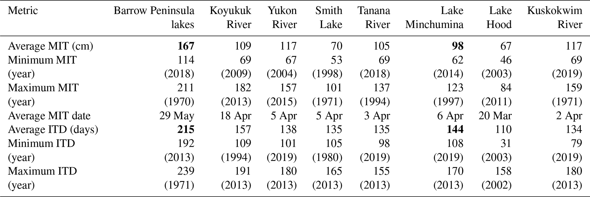
Table 2 Summary of maximum ice thickness (MIT) and ice travel duration (ITD) according to the mean, minimum, and maximum values for each period of record reported here by nearest community to observed lakes and rivers. Years corresponding to minimums and maximums are in parentheses, and metrics with significant trends are in bold.

3 Results

3.1 Patterns and trends in lake ice

Latitudinal patterns in ice thickness exist in Alaska, yet location relative to mountain ranges, river valleys, and coasts, with varying degrees of sea ice influence, likely had a larger influence. Spatial patterns of MIT averaged over periods greater than two decades ranged from 67 cm in Southcentral (Anchorage) and 70 cm in the Interior (Fairbanks) to 167 cm on the Arctic Coastal Plain of northern Alaska (Utqiaġvik) (Table 2). Intermediate average MIT ranged from 98 to 122 cm from shorter-term records collected within the last two decades in western Alaska, along the Alaska Range separating the Southcentral region from the Interior, as well as the Brooks Range foothills of the North Slope (Fig. 1).

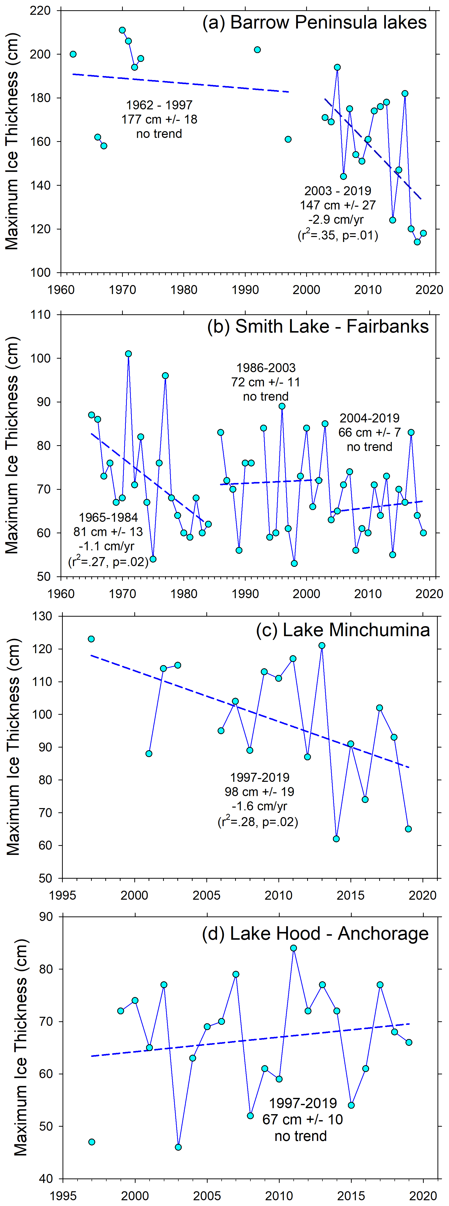
Figure 5 Maximum ice thickness patterns and trends for lakes around the Barrow Peninsula (a), Fairbanks (b), Minchumina (c), and Anchorage (d) for each station's period of record.

Overall the thickest ice and the steepest long-term thinning trend came from lakes on the Barrow Peninsula (Fig. 5a), set between the Chukchi and Beaufort seas (Fig. 1). A significant decrease in MIT from 1962 to 2019 of 0.9 cm yr⁻¹ is most prominent in the period of continuous record between 2003 and 2019 with 2.9 cm yr⁻¹ of thinning (r²=0.35, p=0.01) (Fig. 5a). Analyzed separately, the earlier period with more intermittent observations showed no trend and an average thickness of 177 cm. In comparison, MIT for 4 of the past 6 years was less than 121 cm – a thickness not reported once during the previous 22 years with observations dating back to 1962. MIT on Barrow Peninsula lakes was typically reached between late May and early June, and the average number of safe travel days was 215, with a significant decline of 0.5 d yr⁻¹ (r²=0.54, p<0.01) (Fig. 6). Air temperature during the ice growth season averaged −17.9 ^∘C with an increasing trend over the period of analysis and with temperature above −15 ^∘C during the last 4 of 6 years. Upland snow depth averaged 22 cm with no trend. Winter temperature during the ice growth season explained the majority of variation in MIT for this record (r²=0.61, p<0.01), and upland snow depth was poorly correlated.

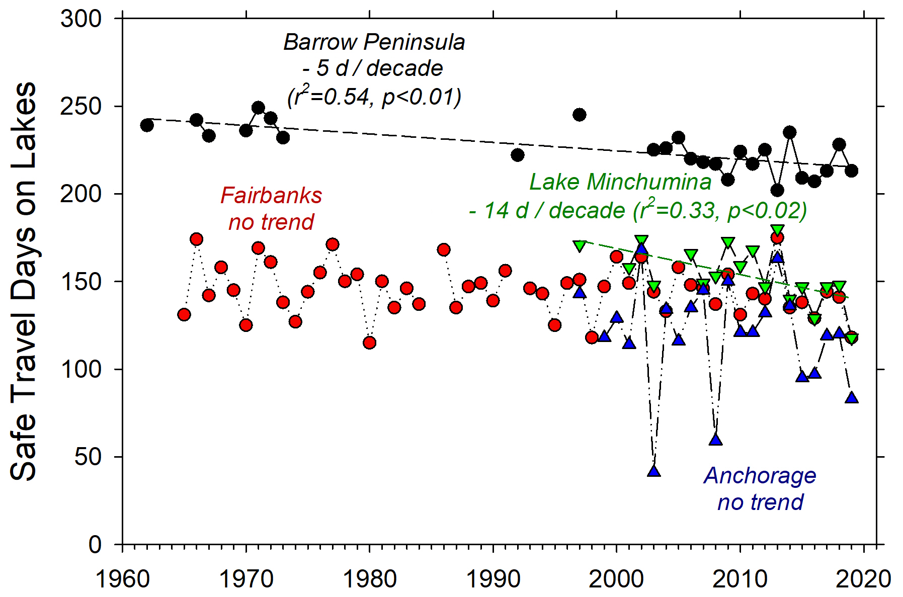
Figure 6 Ice travel duration on lakes estimated from ice growth curves for each period of record.

The next longest and nearly complete record comes from Smith Lake in Fairbanks dating back to 1965 (Fig. 1). Interestingly, no overall trend was observed over this 54-year period, though the two thickest MIT years were in 1971 and 1977. A thinning trend of 1.1 cm yr⁻¹ (r²=0.27, p=0.02) was noted during the first 19 years, while the middle period (1986–2003) had an average MIT of 72 cm, and the last period had average MIT of 66 cm with no trend (Fig. 5b). Very thin MIT, less than 60 cm, occurred in all three periods, and MIT exceeding 80 cm occurred as recently as 2017. Smith Lake is a shallow thermokarst lake with wind-protecting forest around its entire perimeter, typically with relatively deep uniform snow cover. Contemporary synoptic comparisons made by APRFC on several larger and less protected interior lakes within a 100 km radius often show Smith Lake having the thinner ice regionally. Still, Smith Lake may be widely representative of the many small thermokarst lakes and ponds surrounded by forest in interior Alaska. MIT was typically reached by early April, and average ITD was 135 d with no trend over time (Table 2). Air temperature during the ice growth season averaged −16.8 ^∘C with a slight increasing trend, and upland snow depth averaged 36 cm with no trend. Neither upland snow depth nor air temperature during the ice growth season explained interannual variation in MIT or ITD for this lake.

In contrast, the larger and more southerly but slightly higher elevation Lake Minchumina (Fig. 1) had a MIT of 98 cm averaged over 18 years of mostly continuous observation. MIT of this lake became notably thinner over this period, decreasing 1.6 cm yr⁻¹ (r²=0.28, p=0.02) (Fig. 5c). Yet, nearly the thickest MIT in this record, 121 cm, was recent, 2013, and then the thinnest MIT of 62 cm was also recent, 2014 (Table 2). MIT was typically reached by early April, and average ITD was 144 d with a relatively steep declining trend of 1.5 d yr⁻¹ (r²=0.33, p<0.02) over this short period (Fig. 6). We estimated that the most recent year of record 2019 had the shortest ITD of 108 d, while another relatively recent year 2013 had the longest ITD of 170 d (Table 2). The long and relatively cold ice growth season of 2013 was also prominent in other records of ITD in interior sites. Air temperature during the ice growth season averaged −14.8 ^∘C (between Nenana and McGrath stations), with no trend detected.

The most southerly site, Lake Hood, located near the Anchorage International Airport and used as a major floatplane runway, had a similar duration record to Lake Minchumina from 1997 to 2019. Observations on this lake began in 1967, but these appeared anomalously thick, with many exceeding 140 cm and α coefficients averaging 4.8. We suspect that observers may have collected measurements along areas where ski planes or snow grooming compacted the snow significantly to allow this level of thickening with modest winter temperatures. For the period when α coefficients are within a more normal range (1.6–3.7) (Table 1), a nonsignificant increase of 0.3 cm yr⁻¹ was detected with an average MIT of 67 cm (Fig. 4d). MIT was typically reached by late March, and average ITD was 110 d with lots of variation but no trend over this period (Fig. 5). We estimated a very short ITD of 31 d over the winter of 2002–2003 (Table 2) when ice growth only surpassed 30 cm by 31 December and MIT was reached early, on 2 February. That winter, as well as 2007–2008, had numerous freeze–thaw periods through the normal ice growth season, corresponding to short estimates of ITD (Fig. 6). Ice growth season temperature averaged −6.4 ^∘C, and upland snow depth averaged 29 cm, with no trends detected. We suspect snow on this lake would be greatly reduced in some years due to wind scour along with varying alteration from human activities.

3.2 Patterns and trends in river ice

In contrast to lake ice records, fewer river ice thickness records were analyzed in this study. All of these observation sites are on larger rivers within the Yukon and Kuskokwim drainages (Fig. 1), associated with riverside communities. A primary use of these ice thickness data is in forecasting ice jam floods and safe travel conditions. Average MIT over these differing periods of observation ranged from 98 cm on the Tanana River at Nenana (40 years) in the Interior to 117 cm at both the Kuskokwim River at Bethel (57 years) near the Bering Sea and Yukon River at Eagle (20 years) near the Canadian border (Fig. 1).

Figure 7 Maximum ice thickness patterns and trends for rivers near Bethel (a), Nenana (b), Bettles (c), and Eagle (d) for each station's period of record.

Ice observations on the Kuskokwim River began with the CRREL program in 1962 with a decade-long gap starting in 1985 and continued again in 1996 with measurements reported to APRFC. The earlier period (1962–1984) had average MIT of 124 cm with the thickest ice of 159 cm recorded in 1997, no estimates of MIT less than 100 cm, and no trend (Fig. 7a). The second period running to the present also showed no trend but had a somewhat lower average MIT of 111 cm and higher interannual variation than the first period. The thinnest MIT, 69 cm, occurred in 2019 and also corresponded to the earliest river breakup on record, 31 March. Also in contrast to the first period, MIT was less than 100 cm during eight of 24 winters in the recent period (Fig. 7a). However, thick ice (>130 cm) also occurred in 2009, 2010, 2012, and 2017, underscoring a recent pattern of higher interannual variability. The average date of peak ice thickness was 1 April but was estimated to occur as early as February in some years and as late as May in others with no trend. ITD also varied widely from 79 d in 2019 to 190 d in 2013 and averaged 144 d, also with no significant trend (Fig. 8). The Kuskokwim River ice growth curve during the winter of 2018–2019 suggests 30 cm ice thickness was reached by mid-December and MIT was reached in late February. In contrast, during the winter of 2012–2013, 30 cm ice thickness was reached in early November and peaked in early May. During the ice growth period for the full record, air temperature at Bethel averaged −11.8 ^∘C and upland snow depth averaged 14 cm. Neither ice growth controlling condition showed any trend during this period, yet both air temperature and upland snow depth together explained significant portions of variability in MIT (r²=0.24, p<0.03).

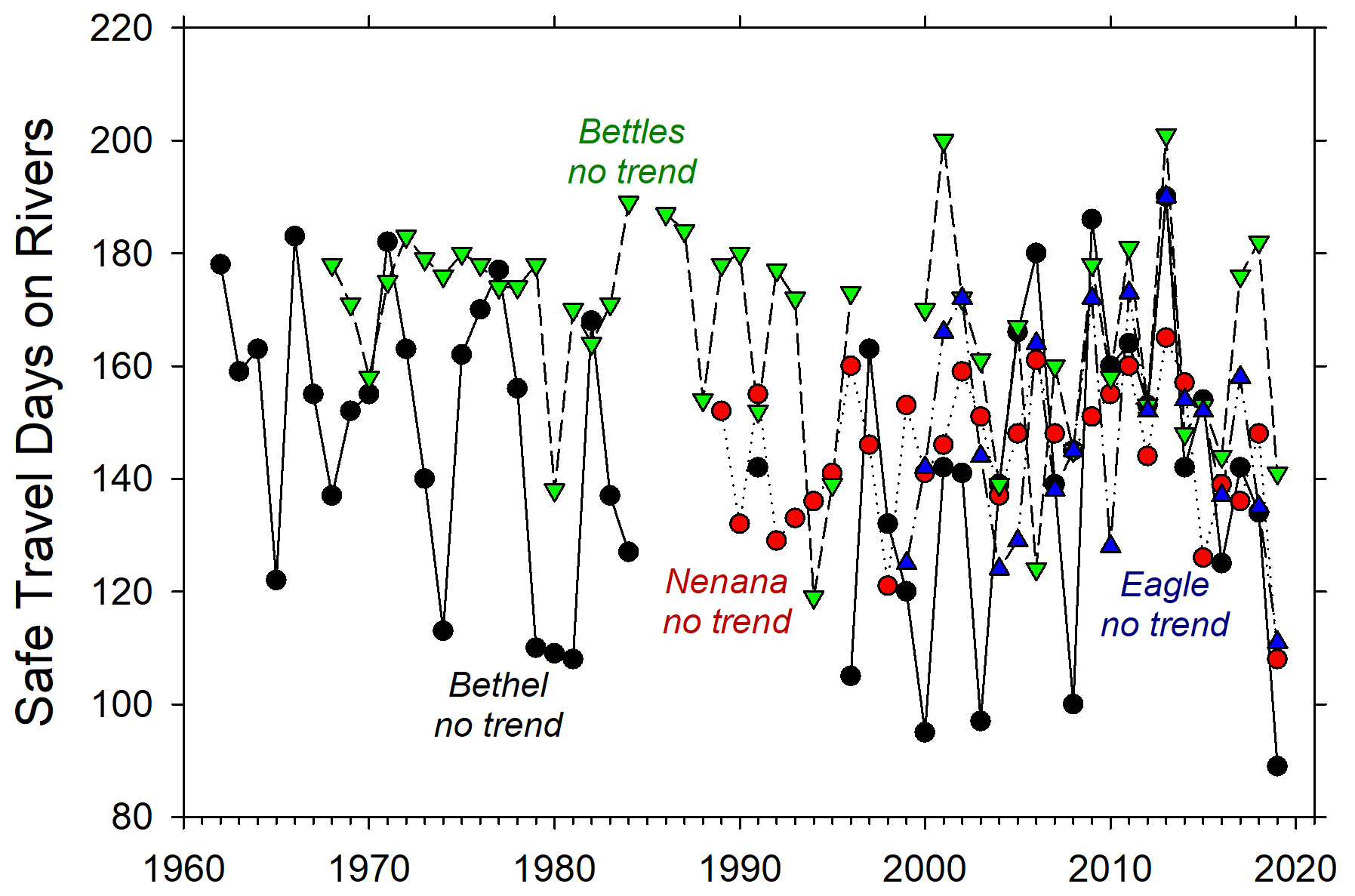
Figure 8 Ice travel duration on rivers estimated from ice growth curves for each period of record.

Ice thickness records on the Tanana River were collected by community members associated with the Nenana Ice Classic (NIC) and were available back to the winter of 1988–1989. In that year, MIT was 112 cm and the average for the entire record is 105 cm (Table 2). The most recent 2 years had the lowest MIT on record, 69 and 72 cm, respectively – the latter, 2019, of which was also the earliest breakup in the 102-year record, tipping the tripod on 14 April. Two distinct ice thickness periods are noted. The earlier period from 1989 to 2007 had average MIT of 106 cm with high interannual variability and no trend (Fig. 7b). The second period showed a strong thinning trend of 4.5 cm yr⁻¹ (r²=0.80, p<0.01) ending in the two thinnest ice years, as previously noted. Ice typically thickened until early April, with recorded breakup happening 1 month later on average. Ice travel duration on this section of the Tanana River averaged 135 d and ranged from 108 d in 2019 to 165 d in 2013 (Table 2) – which also corresponded to the earliest and latest breakup dates for the total 102-year record. Ice growth season air temperature averaged −16.4 ^∘C over this period, and upland snow data were not consistently available at this station over this period.

The second longest and mostly complete river ice observation record was made on the Koyukuk River at Bettles starting in 1968. Three periods were noted in this record of approximately equal durations (Fig. 7c). The first was characterized by increasing thickness of MIT by 3 cm yr⁻¹ (r²=0.33, p=0.02) with ice as thin as 81 cm in 1968 and as thick as 182 cm in 1978. The middle and the latest periods we identified were less distinct in terms of average MIT, 111 and 103 cm, respectively, and lacked trends, but the latter period had much higher interannual variability, with MIT ranging from 69 cm in 2009 to 182 cm in 2013 (Fig. 7c). Ice typically reached its maximum by mid- to late April, and ITD averaged 157 d with less interannual variability than other rivers in this set (Fig. 8). Ice growth season air temperature averaged −18.3 ^∘C, and upland snow was quite deep, averaging 54 cm and ranging from 22 cm in 1996 to 100 cm at the start of the record in 1968. Here, upland snow depth explained a significant portion of the variation in MIT (r²=0.16, p<0.05), while air temperature was uncorrelated to ice variability over this period.

The Yukon River at Eagle showed an increasing trend in MIT of 1.5 cm yr⁻¹ (r²=0.17, p=0.06) from 1999 to 2019, though not quite significant statistically (Fig. 7d). Three distinctly thin ice years occurred in 1999, 2004, and 2019 when the MIT reached 82 cm or less. Recent thick ice years in 2015 and 2017, when the MIT was greater than 150 cm, contributed to this weak trend of increasing ice growth (Fig. 7d) at this easternmost station near the Canadian border. MIT was typically reached in early April in most years, and ITD ranged from 101 d in 2019 to 180 d in 2013 (Table 2). Air temperature during the ice growth period averaged −16.5 ^∘C and was not correlated with variation in MIT over this period. Upland snow observations were not consistently recorded at the station in Eagle.

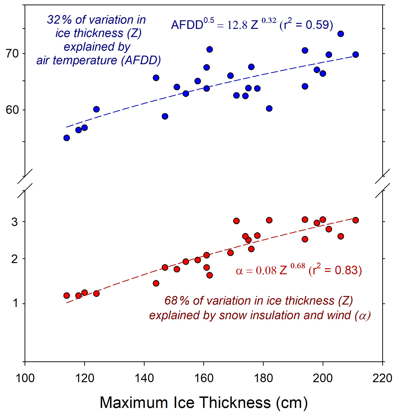
Figure 9 Example from Barrow Peninsula lake data using power law analysis partitioning of variation in MIT (Z) (Eqs. 3 and 4) balanced between air temperature (AFDD) and snow insulation (α).

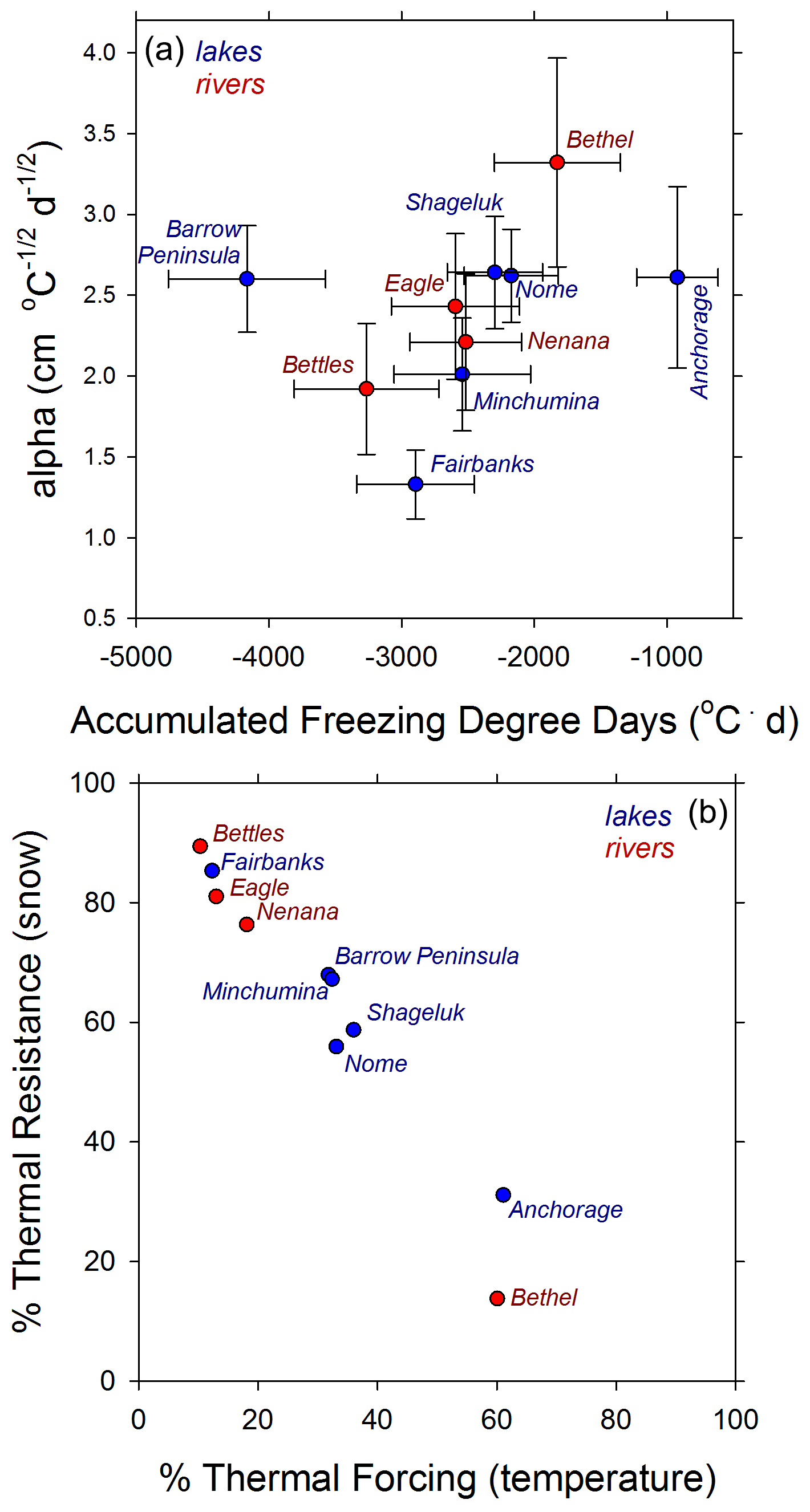
Figure 10 Comparison of mean (±1 SD) alpha and accumulated freezing degree day parameters for MIT records in lakes (blue) and rivers (red) (a) and the proportion of variation explained by thermal resistance and thermal forcing (b).

3.3 Controls on ice growth

Estimating rates of ice growth across a wide set of lakes and rivers and many years based on late winter ice thickness observations and air temperature data produced a correspondingly wide range of α coefficients and AFDD values (Table 1). Though not widely reported or analyzed in ice thickness literature, α values typically range from 0.4 for snow-covered rivers to as high as 2.7 for snow-free lakes. For coastal plain lakes on the Barrow Peninsula, where we have the widest range of variation in MIT (Fig. 5a), partitioning of variation using power law analysis suggests that 32 % is explained by AFDD and 68 % is explained by α (Fig. 9). Comparison of average α and AFDD values for all lake and river records are presented together in Fig. 10a. Here, α values for lakes in windy coastal regions were all close to 2.6, with the most interannual variability noted for Lake Hood in the southernmost site in Anchorage. The interior lakes studied had average α values of 1.3 in Fairbanks and 2.0 in Lake Minchumina, likely relating to less wind and more consistent deep snow packs. River ice α values were much higher than suggested in the literature, with averages ranging from 1.9 in Bettles with very deep snowpacks up to 3.3 in Bethel where snowpacks are thinner and highly wind affected. Though exact data on snow-ice formation and overflow contributions to ice thickness are not consistently reported in most ice observation data, we suspect that very high α coefficients correspond to such processes on rivers. Analyses of factors controlling ice growth consistently point towards the dominant role of snow in determining maximum ice thickness in most lake and river settings (Fig. 10b) according to interannual variability in thermal forcing as described by AFDD and thermal resistance as described by α using Eqs. (3) and (4), respectively. Analysis of Bethel and Anchorage sites, however, show that variations in air temperature may be the more important factor for these southernmost, coastal settings (Fig. 10b).

The majority of ice thickness data we report here do not have coincident measurements of snow depth or snow density. An exception was ice thickness data collected by the CALON project on Alaska's North Slope between 2012 and 2016, where observations of ice thickness and snow depth and density were made in late winter close to the time of maximum ice thickness. Short-term air temperature records collected adjacent to study lakes also enhanced the accuracy of ice growth curve analysis and estimation of parameters. Thus, this dataset presents an opportunity to make closer comparisons of snow characteristics to the heat exchange coefficient α. Increasing snow depth and decreasing snow density reduce heat loss and slow ice growth, such that a simple snow insulation index (SII) can be presented as the ratio of snow depth to density. Comparing this SII to α for this North Slope MIT dataset suggest several tight and interesting patterns (Fig. 11). The combination of snow depth and density as SII explained between 94 % and 98 % of variation in the heat exchange coefficient α but followed two distinct separate linear relationships (Fig. 11). The steeper relationship of decreasing α with increasing SII appeared to correspond to lake snowpacks of moderate depth (15–30 cm) and higher densities (30–40 g cc⁻¹). For deeper snow and/or lower-density snow, this relationship was also tight, with a shallower slope over this wider range of SII (Fig. 11). One outlier corresponded to high α and very low SII due to very thin and dense snow cover on a lake most likely due to intense wind scour. Distinction between the two linear groupings may be generally explained by wind regimes experienced by those lakes in those years as well, though this was not analyzed distinctly. Development of SII data for other lakes or river records was not available to make similar comparisons.

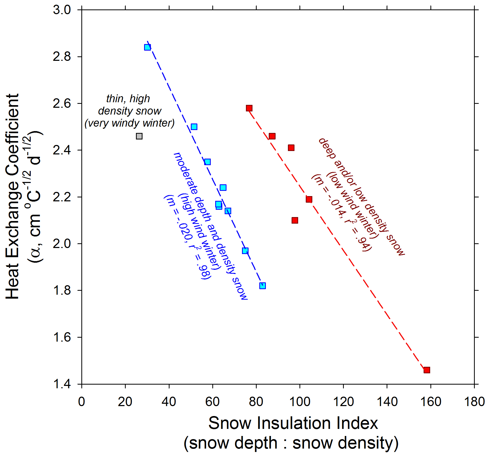
Figure 11 Explanation of variation in the heat exchange coefficient (α) for North Slope lake ice near late winter MIT according to a proposed snow insulation index (snow depth in cm and snow density in g cm⁻³). Distinct patterns emerged for snow conditions expected for low-wind vs. high-wind winters, which may be applicable to other environments.

4 Discussion

The clearest signal of reduced ice growth and shorter-duration ice cover come from lakes in northern Alaska where the impacts of arctic amplification are known to be most pronounced (Wendler et al., 2014; Walsh and Brettschneider, 2019). The majority of this trend from Barrow Peninsula lakes is driven by recent declining sea ice impacts on early winter temperature and snowfall (Alexeev et al., 2016), though strong interannual variability in ice thickness is still evident (Arp et al., 2018). Barrow Peninsula ice observations from 1962 to 1996 are well within the range of more distant single-year observations of 192 cm in 1955 (Brewer, 1958) and 188 cm in 1882 (Ray, 1885). In comparison, MIT for 4 of the past 6 years was less than 121 cm – a thickness not reported once during the previous 22 years with observations dating back to 1962. Snow is typically considered the dominant control on interannual variability in ice thickness for coastal plain lakes (Zhang and Jeffries, 2000), yet warmer winter temperatures during the ice growth season appear to have overcome this driver of ice growth in our analysis, at least when comparisons are made using upland snow records. Snow depth on coastal plain lakes is typically about 60 % of upland depth on average (Sturm and Liston, 2003), but this can vary greatly from year to year (Arp et al., 2018), and this changing offset between tundra snow and lake snowpack may explain the lack of correlation to upland snow records we observed. Partitioning the relative roles of air temperature vs. snow insulation on lakes, however, still suggests that snow is the dominant factor in lake ice variability (Fig. 9). The role of arctic amplification and early winter warming is also seen in reduced safe travel days on ice for Barrow Peninsula lakes (Fig. 6a), with the majority of this decrease coming from slower ice thickening rather than earlier arrival of MIT.

Despite the impacts of arctic amplification on winter climate change in other parts of Alaska (Walsh and Brettschneider, 2019), the response of river and lake ice growth in several records spanning over 50 years often appears muted or highly variable. Such variation appears evident in the analysis of the relative roles of thermal resistance due to snow and thermal forcing due to air temperature (Fig. 10a), suggesting differing process controls on ice growth across regions and among lakes and rivers. In western coastal Alaska, recent thin ice conditions and short ice cover duration on the Kuskokwim River were striking yet follow a pattern of enhanced variability over recent decades. Thin ice conditions of the 2018–2019 winter were observed in nearly all records we analyzed and provided much of our motivation to standardize, summarize, and analyze these records. In contrast, the relatively recent winter of 2012–2013 had consistently thick ice and very prolonged ice cover duration across western and interior Alaska. Such dramatic winter conditions and divergent ice responses underscore the need for enhanced freshwater ice observation programs.

The premise that freshwater ice growth integrates changes in climate deserves consideration (Allen, 1977; Engram et al., 2018). We found few consistent relationships between fundamental drivers of ice growth, air temperature, and snow depth, suggesting that other more complex environmental factors play a role in river and lake ice dynamics. One factor is that snow accumulation on ice is fundamentally different than terrestrial upland snowpacks where snow depth is recorded – typically ice on rivers and lakes is thinner and depending on the ice column's isostatic balance can slow ice growth through insulation or thicken it through formation of snow ice and overflow (Sturm and Liston, 2003; Ashton, 2011). Particularly on rivers, the combined hydrologic and thermal conditions of flowing waters can also cause divergent responses in ice thickness – more and warmer water can cause slower growth or degradation but also generate overflow that can refreeze and add thickness to ice covers (Prowse and Beltaos, 2002; Brown and Duguay, 2010; Jones et al., 2015). Little is known about changes in groundwater in Alaska, which also impacts ice growth on rivers, though several studies do point to increases in groundwater input (Brabets and Walvoord, 2009; Liljedahl et al., 2017). Higher water temperatures in relation to enhanced groundwater input present another potentially important driver affecting ice growth and decay that deserves evaluation (Jones et al., 2015; Cherry, 2019). Many of these interactions are documented by process studies of lake and river ice (Ashton, 2011), and observations of these processes also appear sporadically in monitoring program notes (Bilello, 1980) but are challenging to quantify in long time-series analyses such as this one. Thus, ice thickness at its seasonal maximum (MIT) and duration of the ice growth season (ITD) do integrate important and complex changes in climate including the hydrologic cycle, but these responses do need to be carefully interpreted and compared along with other environmental drivers.

This analysis of long-term ice observation records in Alaska using standardized metrics from ice growth curves provides an important baseline to compare with future observations and support process studies. Past freshwater ice observations programs in Alaska, including CRREL (Bilello, 1980) and ALISON (Morris and Jeffries, 2010), both collected basic ice thickness data that supported numerous process studies adding to our ice dynamics predictive capability (e.g., Jeffries et al., 2005; Arp et al., 2010: Ashton, 2011). These datasets are now archived by the Arctic Data Center (http://arcticdata.io/, last access: 1 December 2019) as Bilello (2019) and Morris and Jeffries (2019), and many of these records continued and are made readily available by APRFC (https://www.weather.gov/aprfc/IceThickness, last access: 1 March 2020). A new freshwater ice observation program, Fresh Eyes on Ice (http://freshiceonice.org, last access: 1 March 2020), is working to continue monitoring and analysis of river and lake ice conditions in Alaska in part through engagement with rural communities and schools using a combination of approaches including remote sensing and field-based observations. The strong and interesting relationships observed between ice growth and snow characteristics for North Slope lakes (Fig. 11) may provide guidance and incentive to collect more complete snow data to inform modeling and prediction of ice growth in other regions as well. The employment of temperature-driven ice models that could be refined based on known or expected snow cover conditions may provide an opportunity for near-real-time estimates or even forecasts of ice conditions in remote regions of Alaska. Incorporation of community-based monitoring into such efforts may not only advance more comprehensive data collection, but also promote the use of new ice products in making safe travel decisions.

Our analysis of ice growth curves only represents a portion of the ice formation, growth, and decay process, whereas more abundant ice phenology studies (e.g., Arp et al., 2013; Cooley and Pavelsky, 2016; Smejkalova et al., 2017; Sharma et al., 2019; Yang et al., 2020) identify patterns and trends at the very start and very end of this cycle of seasonal ice cover. Perhaps the two most relevant and also challenging periods are (1) the period from initial freeze-up to ice of sufficient thickness to supporting most modes of travel (e.g., <30 cm) and (2) the period when ice-surface snow is completely melted (when ice decay fully initiates) to breakup. These periods in terms of process can vary greatly in length and spatial variability, both of which have great importance for informing travel conditions and should be viewed as a continuum rather than momentary to-the-day events (Brown et al., 2018). The critical freeze-up period occurs from when ice first forms and grows on water surfaces to when ice cover is spatially consistent and thick enough to support reliably safe travel. The critical breakup period starts after reaching MIT and then once snow cover is reduced to the point when ice can be exposed to direct solar radiation and decay begins to proceed more rapidly, though often it proceeds at widely varying rates in space and time for lakes and even more so for rivers. The importance of understanding how these periods of freeze-up to continuous thick ice and decay initiation to breakup progress, and how this progression may be changing over time, is critical in terms of informing safe winter travel, predicting ice jam flood hazards, and understanding interactions with river and lake ecosystems (Brown et al., 2018). Focusing on these key ice growth and decay periods and how they may be responding in new ways to climate change and arctic amplification deserves renewed attention in northern regions.