the Creative Commons Attribution 4.0 License.
the Creative Commons Attribution 4.0 License.
 | 26 Oct 2020
Observations of sea ice melt from Operation IceBridge imagery
Nicholas C. Wright
Chris M. Polashenski
Scott T. McMichael
Ross A. Beyer
The summer albedo of Arctic sea ice is heavily dependent on the fraction and color of melt ponds that form on the ice surface. This work presents a new dataset of sea ice surface fractions along Operation IceBridge (OIB) flight tracks derived from the Digital Mapping System optical imagery set. This dataset was created by deploying version 2 of the Open Source Sea-ice Processing (OSSP) algorithm to NASA's Advanced Supercomputing Pleiades System. These new surface fraction results are then analyzed to investigate the behavior of meltwater on first-year ice in comparison to multiyear ice. Observations herein show that first-year ice does not ubiquitously have a higher melt pond fraction than multiyear ice under the same forcing conditions, contrary to established knowledge in the sea ice community. We discover and document a larger possible spread of pond fractions on first-year ice leading to both high and low pond coverage, in contrast to the uniform melt evolution that has been previously observed on multiyear ice floes. We also present a selection of optical images that capture both the typical and atypical ice types, as observed from the OIB dataset. The derived OIB data presented here will be key to explore the behavior of melt pond formation Arctic sea ice.
- Article
(25795 KB) - Full-text XML
-
Supplement
(2238 KB) - BibTeX
- EndNote


The extent and age of the Arctic sea ice cover have declined since the beginning of the satellite record in 1979 (Stroeve et al., 2012). Ice melt is accelerated through albedo feedback cycles initiated by surface melt decreasing the ice cover's reflectance (Curry et al., 1995; Perovich et al., 2003). Understanding changes in sea ice properties that impact albedo, particularly melt pond coverage, is important to parameterizing sea ice in global climate models (Hunke et al., 2013; Serreze et al., 2009). In situ observations that could support developing this understanding are sparse, difficult to acquire, and may not be broadly representative (Perovich, 2002; Wright and Polashenski, 2018). Remote sensing platforms provide a path to understanding sea ice surface change over larger scales. Newly developed computational techniques provide the means to analyze large remotely sensed datasets (Miao et al., 2015; Webster et al., 2015; Wright and Polashenski, 2018). The NASA Operation IceBridge project (OIB) has collected large amounts of high-resolution optical imagery of sea ice with the Digital Mapping System (DMS) (Dominguez, 2010, updated 2017). At ∼10 cm resolution, these images capture the ice surface in fine detail – but it is challenging to convert them to quantitative measures of ice conditions.
A new technique for analyzing high-resolution optical imagery of sea ice has recently been developed and demonstrated (Wright and Polashenski, 2018). This technique, named the Open Source Sea-ice Processing algorithm (OSSP), automatically analyzes input imagery and classifies image area into four primary surface type categories: (1) snow and unponded ice, (2) dark or thin ice, (3) melt ponds and submerged ice, and (4) open ocean. Categories 1 and 2 are often combined to create a unified ice category. Several improvements and new features that define version 2 of OSSP are presented here. This version was used to create a new dataset by deploying the algorithm on a large scale to process the entirety of the NASA OIB optical image dataset. This dataset is now publicly available for community use and for other studies leveraging the IceBridge data suite. This publication is intended partially to serve as supporting documentation for those uses.
The summer portion of the new dataset is then used to evaluate existing hypotheses about melt pond formation on Arctic sea ice. One such hypothesis describes the prevalence of ponds on first-year sea ice (FYI) versus multiyear ice (MYI). It has been widely stated that FYI has a higher average fractional pond coverage than MYI over the complete melt season (Eicken et al., 2004; Fetterer and Untersteiner, 1998; Morassutti and Ledrew, 1996; Perovich and Polashenski, 2012). This would contribute to positive ice–albedo feedbacks, since the higher pond fraction would lower albedo of FYI, reenforcing the transition to a younger ice pack. The reasoning most cited for expecting higher pond coverage on FYI is related to ice and snow topography (Barber and Yackel, 1999; Derksen et al., 1997; Eicken et al., 2004). When ice grows from open Arctic waters, it tends to form in flat, undeformed pans or fairly level pancake fields. Though these pans are subsequently broken and ridged by dynamic forces, in most parts of the Arctic a large fraction of FYI remains level. When surface melt begins on level FYI floes, meltwater is unconstrained by topography and spreads to cover a large fraction of the surface. On MYI, however, the ice has survived prior melt seasons that create more complex surface topography even in areas without mechanical deformation. The meltwater is then contained by the prior year's melt-formed topography into well-defined pools. The result should be that FYI would tend to experience greater pond coverage than MYI. Indeed, this has been presented by several authors as a likely change in the Arctic (Eicken et al., 2004; Polashenski et al., 2012).
It is important to note that pond evolution over the melt season is highly variable and is controlled by the balance of meltwater inflow and outflow rates, surface topography, and snow depth. There are four stages that characterize seasonal melt pond formation described in Eicken et al. (2002) and paraphrased as follows. (1) Initial onset of ponds above sea level with a rapid increase in areal coverage, (2) increased outflow allowing drainage to sea level with a decline in areal extent, (3) gradual increase in areal coverage due to ice melting to below ocean freeboard, and (4) refreezing. Despite a common understanding of high pond coverage on FYI, a collection of previous observations (Eicken et al., 2004; Perovich, 2002; Webster et al., 2015) have shown the possibility that FYI has lower pond coverage than MYI under certain circumstances. For example, in stage 2 areal coverage drops significantly more on FYI than it does on MYI (Polashenski et al., 2012). Observations at the SHEBA drifting ice camp found that 10 %–30 % of the FYI in the region formed few melt ponds. Measurements there linked this observation to snow cover: ice with little or no snow cover and with more than 0.5 m snow cover had less than 1 % pond coverage (Eicken et al., 2004). Webster et al. (2015) found regions where FYI started ponding much later than MYI, though the FYI ultimately developed higher pond coverage later in the summer. A new observational dataset of melt ponds on sea ice from OIB is used here to assess pond coverage differences between ice age at the height of summer melt (July) and to expand previous observations of pond-free FYI to regional scales.
A second, related, hypothesis on the behavior of FYI melt ponds suggests two summer melt evolution pathways exist: one which yields high pond fraction and one that yields near-zero pond fraction (Perovich, 2002; Polashenski et al., 2017), depending on early season ice permeability and the duration of surface flooding. Our new observations of pond coverage over large areas of FYI provide additional insight. Here, the OSSP-labeled OIB images were used to assess the variation in pond coverage on FYI and the prevalence of pond-free floes within the Chukchi and Beaufort seas. To accomplish this, a method of post-processing has been developed that determines the size of sea ice areas devoid of pond coverage as a metric to quantitatively address the prevalence of low pond coverage. This new analysis reveals that FYI pond coverage indeed exhibits both pathways but that there is not a strict duality – FYI pond coverage appears to occupy all states across the near-zero to high-coverage space. While the OIB image dataset provides large spatial coverage over long flight transects, the lack of temporal coverage makes it impossible to directly link these snapshots of pond coverage to any specific pond evolution process.
2.1 Data sources
The datasets described herein are the result of processing NASA Operation IceBridge optical DMS imagery. The DMS images were acquired with a Canon EOS 5D Mark II digital camera which has a 10 cm horizontal ground resolution and a spatial footprint of ∼600 m × 400 m when used at the survey altitude of 1500 ft (457 m) (Dominguez, 2010, updated 2017) and is available for download at the National Snow and Ice Data Center (NSIDC). A total of 87 IceBridge flights were processed, occurring between 2010 and 2018. The OIB flights were categorized into freezing and melting conditions, which map to the spring–fall and summer campaigns, respectively. The mean date of melt onset in the Chukchi Sea, Beaufort Sea, and central Arctic from 1979 to 2012 was 17 May, 28 May, and 10 June, respectively (Bliss and Anderson, 2014). Spring flights took place before these dates (March to mid-May, typically) and summer flights well after (middle to late July). No flights took place during melt or freeze onset transitional phases, making this a clean categorization. The flights between March and May were categorized as freezing condition flights (no melt ponds expected), and those taken in July were categorized as melting condition flights (melt ponds expected). One flight during fall freeze-up (5 October) was processed and was grouped with the spring set. Using this delineation, there were nine flights during melting conditions and 78 flights during freezing conditions. Of the nine melting condition flights, five occurred in 2016 originating from Utqiaġvik, Alaska, and four occurred in 2017 originating from Thule AFB, Greenland. There was an additional summer flight departing from Utqiaġvik on 20 July 2016 that was not processed due to constant cloud cover obscuring the images.
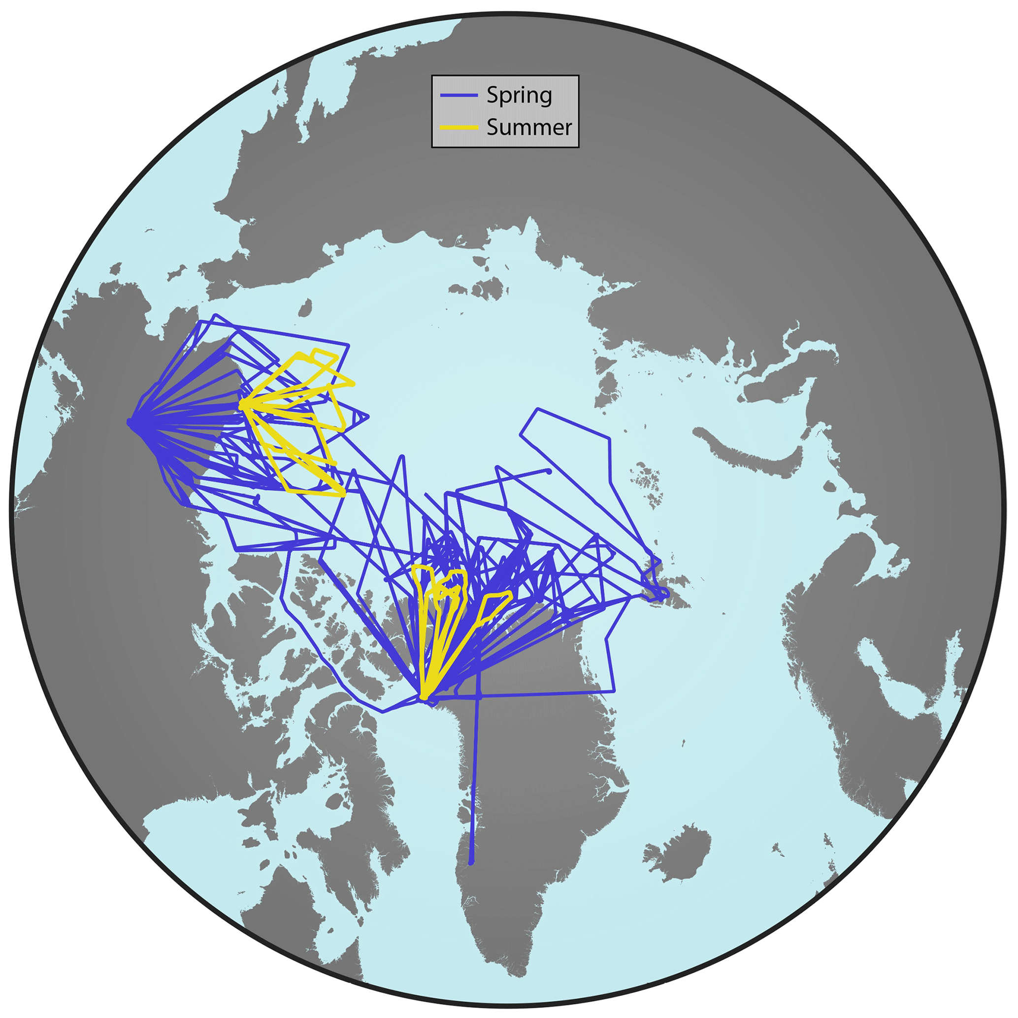
Figure 1Plot of all flights processed with OSSP, colored by the melt conditions during the flight. Spring freezing conditions are shown in blue, and summer melting conditions are shown in yellow. Coastline data were derived from © OpenStreetMap contributors 2020. Distributed under a Creative Commons BY-SA License.
A graphic of the flight tracks for all OIB sea ice flights processed, colored by freezing–melting condition status, is presented in Fig. 1. For the majority of this paper, we will focus on the melting season (summer) flights, colored in yellow. Spring data products are posted for use by the community. We anticipate that future analysis of spring flight data will help confirm lead identification in analysis of altimetry data and provide statistics on lead size and spacing and morphology useful to studies of, for example, blowing snow loss to leads or ice dynamics.
2.2 OSSP algorithm improvements
A number of improvements have been made to OSSP since the initial version 1 release described in Wright and Polashenski (2018). These changes can be divided into three categories: (1) those that alter the algorithms used to classify images, (2) those which add new features, and (3) those which improve code efficiency but do not alter the core methodology. Changes that fall into category (3) reimplemented existing functions for improved performance and decreased computational resource usage. These will not be discussed in detail as they do not change the results.
2.2.1 Algorithm refinements
OSSP is an object-based segmentation and classification image processing algorithm. In version 1, edge detection for segmentation was done by applying a Sobel–Feldman filter to the image, amplifying the resulting values to highlight strong edges and thresholding low-gradient-value pixels to remove weak edges. The amplification factor and threshold value were both presented as tuning parameters that could control the number and strength of edges to detect in the image. In version 2, image edges are instead found with a Canny edge detector (van der Walt et al., 2014), which has three built-in tuning parameters: a Gaussian filter with a chosen radius that removes noise from the image, a high threshold which selects strong edges, and a low threshold which defines weak edges. These three parameters can be selected based on the quality of the input image and the degree of segmentation sought. The change in edge detection method does not significantly shift the behavior of the OSSP method but allows the user to better tune the segmentation to specific images. The remainder of the OSSP code uses methodology as presented in Wright and Polashenski (2018).
2.2.2 New features
Four new features were added for processing the OIB optical image dataset: (1) an image quality analyzer which flags excessive cloud cover or haze, (2) an automatic white balance correction function, (3) expanded training datasets specific to OIB images, including shadow detection in spring images, and (4) orthorectification to a flat plane WGS84 spheroid.
Clouds and semiopaque haze are common in OIB imagery. These often partly obscure the surface and prevent accurate image classification. An automated algorithm has been added that detects obscured images so that they can be removed from analysis. The quality check is based on applying a Fourier transformation to the image to detect the ratio of high- and low-frequency features. It is an implementation of the De and Masilamani (2013) method, where the quality score is the percent of image pixels that have a frequency greater than 1∕100 000 of the maximum frequency. Poor-quality images were empirically found to have a score of less than 0.025, potentially unusable images had a score between 0.025 and 0.035, and images with a score greater than 0.035 were generally acceptable.
A large number of OIB images are taken in poor-surface-lighting conditions. This is often a result of the aircraft flying under cloud cover or high solar zenith angles. Darker-than-expected and blue-shifted images are observed under these conditions. Unlike the hazy images flagged by the quality check, these can still be accurately classified. An automatic white balance correction function has been added to standardize the hue and exposure of these images and the resulting image classification. We use a single-point white balance algorithm:
where and is a chosen white reference pixel, (R,G,B) is the original pixel value triplet, and is the corrected pixel value triplet. The reference point triplet is chosen automatically based on the image histogram of each color band; it is the smallest value that is both larger than the highest intensity peak and has less than 15 % of that peak's pixel counts. This method sets the selected reference point to true white (255,255,255). All other pixels in the image are corrected with the same linear scaling which serves to both adjust the image exposure and rebalance the RGB ratios. The white reference pixel is limited to a minimum value of 200 for images with only a single surface. This prevents them from being improperly stretched so that an open-water-only image will remain black. The effect this color correction has on two poorly illuminated images is shown in Fig. 2.

Figure 2Demonstration of the image preprocessing steps. The raw images (a, b) have poor surface illumination and a blue hue which have both been removed in the standardized images (c, d).
The OIB dataset has a clear binary division between flights where melt ponds are expected (July) and those where they are not (March–May). This characteristic allows for the utilization of two specialized training datasets – one for each season. The summer training dataset is a new, larger set than was presented along with OSSP v1.0, including additional points to encompass a wider range of possible ice conditions. The spring training dataset includes a ridge shadow surface classification class and does not include a melt pond category. The shadow detection method was not applied to melting condition images as the typical summer solar zenith angle yields fewer shadows. The algorithm allows melt pond and shadow detection to be used together given the correct training data, but this was not utilized for the creation of the dataset described here. Webster et al. (2015) found that ridge shadows make up less than 0.5 % of the ice surface in spring, indicating that any errors due to misclassifying them are small. Removal of the melt pond category from spring images prevented occasional spurious detection of melt ponds and improved the quality of results. The training data creation followed the same technique presented in the OSSP version 1.0 documentation (Wright and Polashenski, 2018). The summer dataset was expanded to a total of 1706 training points and the spring dataset to a total of 865 points. These training datasets can be found along with the OSSP code at Zenodo (https://doi.org/10.5281/zenodo.3551033, Wright and Polashenski, 2019).
2.3 Detecting pond-free ice areas
The labeled image output by the OSSP algorithm was further analyzed to extract metrics about the spatial distribution of water features in summer. A technique was developed to find contiguous regions of pond-free ice. These regions were defined as a circle with a diameter greater than 12 m that does not overlap any water feature. First, the labeled image was converted into a binary image separating the snow and ice features from water (i.e., melt ponds plus ocean). Next, the distance from every snow/ice pixel to the nearest water feature was calculated, and peaks with a local maximum distance above a threshold of 12 m were recorded. Pond-free areas are the circle centered at these peaks with a radius of the distance to the nearest water feature. Any two overlapping regions were combined by adding the non-overlapping area of the smaller region to that of the larger region. These pond-free regions are divided into two categories, small and large, based on a threshold of a 25 m radius. The thresholds of 12 and 25 m were selected to be approximately 2× and 4× the mean caliper diameter of melt ponds (Huang et al., 2016). The number of pond-free areas per image was multiplied by the ice fraction (sum of all non-ocean categories) of that image to account for differing ice concentrations between images. Figure 3 shows an example of this detection, where the locations of both the small and large regions are marked with small dots, and the large regions have a translucent circle showing the size of that region.

Figure 3Example of the pond-free region detection. Pond-free regions are marked by small colored dots. Blue dots indicate the larger regions and orange dots indicate the smaller ones. Translucent blue circles are drawn with a radius equal to the size of the detected large regions. Blue dots without a translucent circle were merged with a neighboring region.
2.4 Error
There are several sources of error in OSSP ice type classifications when applied to the DMS dataset. The established accuracy of the OSSP method, on a high-quality input image, is 96 % (Wright and Polashenski, 2018). The principle source of error novel to this OIB dataset was due to lower-quality images, typically from haze obscuring the surface or poor surface illumination. While automated methods standardize the quality of the input and flag bad images (Sect. 2.2.2), some input errors remain. The impact of uncorrected haze is twofold. First, it causes the algorithm to misclassify open water as melt pond, and second, it obscures surface type boundaries and causes insufficient image segmentation. Both issues can be understood by looking at how haze changes an optical image: it adds noise to the image, tends to brighten the pixel values, and blurs surface features. As the defining feature of open water is its uniform darkness, a layer of haze makes this surface more like a dark melt pond. The blurring impacts the edge detection algorithm used by OSSP and therefore causes a breakdown of the proper delineation of image surfaces. For the analyses of the summer dataset presented herein, images were manually sifted to remove those scenes that were not flagged by the quality check algorithm (Sect. 2.2.2) but were still of questionable quality. Due to the heterogenous nature of sea ice, there is a trade-off between accuracy on a specific image and accuracy on the entire dataset – some images flagged as low quality may be usable with a training dataset tailored to those specific images. Users of this dataset should inspect their region of interest to ensure the image quality meets their desired standard.
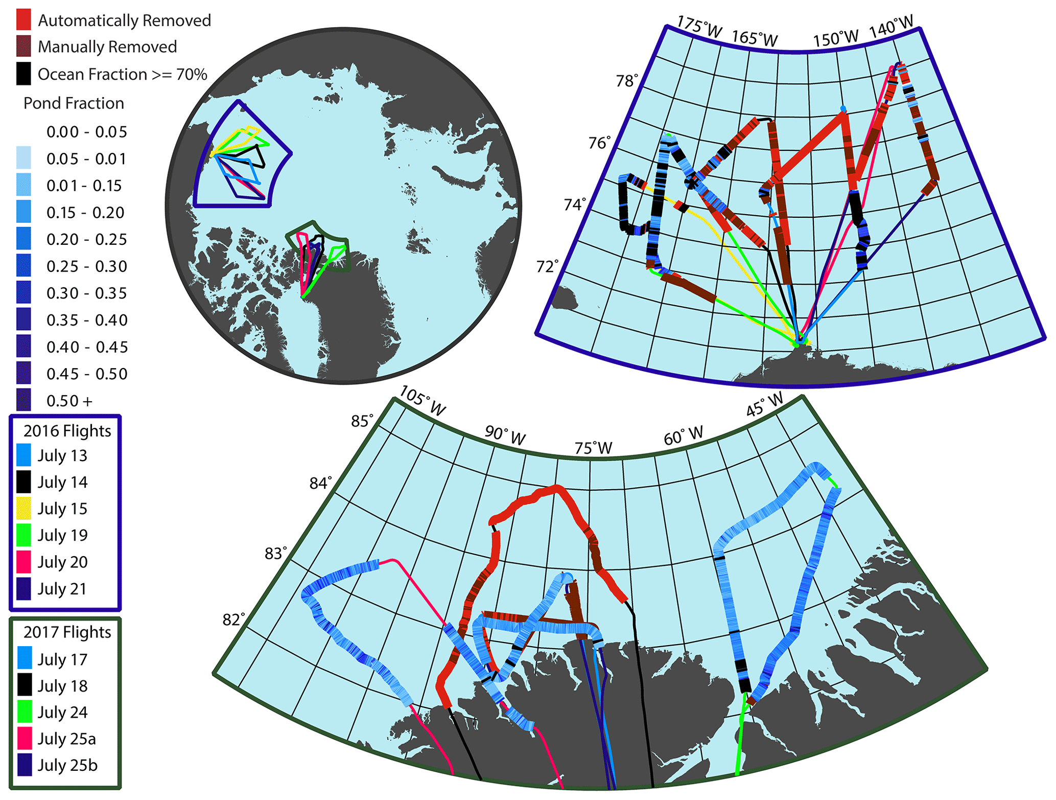
Figure 4Melt pond fraction along OIB summer transects. Automatically and manually removed images are indicated by bright red and dark red, respectively. The 2016 flights were more prone to haze obscuring the ice surface, and therefore a large larger number of images had to be removed. Coastline data were derived from © OpenStreetMap contributors 2020. Distributed under a Creative Commons BY-SA License.
3.1 Melt pond fraction along OIB flight tracks
In this paper we focus on presenting results from summer images only. Images from 87 IceBridge flights were processed with the OSSP algorithm representing over 900 000 individual images using the methods described above – these results are available for other investigations at the NSIDC archive. Figure 4 maps the track of every melt season OIB flight and plots melt pond fraction observed along these tracks. Melt pond fraction was calculated as the number of melt pond pixels divided by the total ice area (ice pixels + pond pixels). Images where more than 70 % of the area was classified as open water are colored black in Fig. 4 but were processed normally. Images that were automatically removed due to a low quality score (Sect. 2.2.2) are colored bright red, and images that were manually removed due to low image quality are colored dark red. In total, 40 672 summer images were analyzed, of which 14 876 (36.6 %) were flagged with a low quality score, 5671 (13.9 %) were manually removed, and 20 125 (49.5 %) were kept for this analysis. The 20 July 2016 flight was not processed because only about 2 % (30 total) of the images were haze free. Note both high variation in pond coverage along track and general regional changes between flights. Some additional variation between flights is due to temporal change; for example it appears a summer snow occurred just prior to the 19 July 2016 flight, lowering the observed pond fraction.
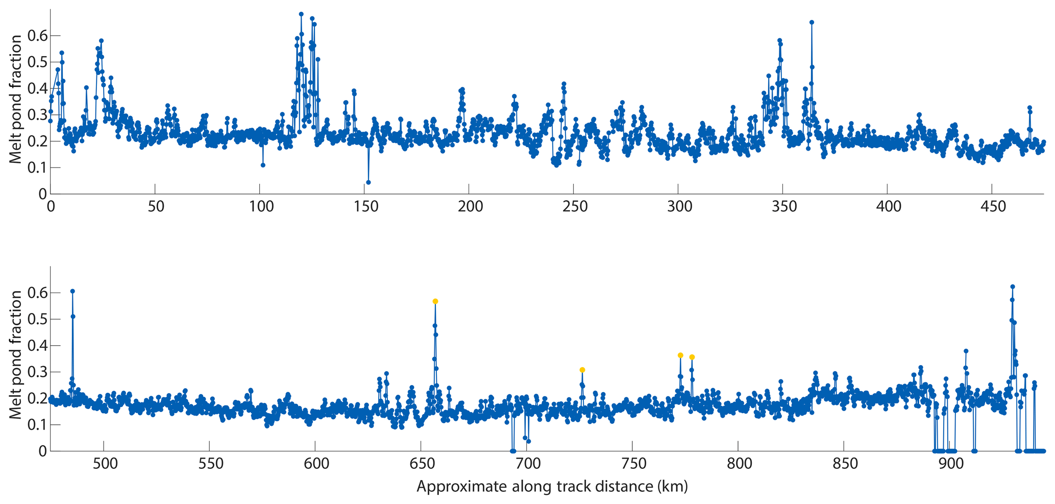
Figure 5Melt pond fraction along track for flight 24 July 2017. The four orange highlighted points represent areas where there was a large blue pond on the multiyear ice that occupied a large fraction of the image. See Fig. 11d for an example of this feature.
Figure 5 plots 300 km of the along-track melt pond fraction for the 24 July 2017 flight. This figure illustrates the large variability possible in melt pond fraction along track seen in the first half of the flight (top), with a minimum observed fraction of 10 % and spikes to greater than 50 %. The second half of this flight (bottom) has a more uniform melt pond fraction of ∼20 %. Four peaks are highlighted in orange where a large blue pond formed on the MYI (see Fig. 11d). Figure 6a zooms in to a 10 km subset of this transect, and the surface corresponding to the orange highlighted section is shown in Fig. 6b. The optical image is the result of stitching 23 DMS images together. The highlighted peak in melt pond fraction occurs on a section of FYI between two multiyear floes. This case follows the prevailing hypothesis about the differences between pond formation on MYI and FYI. The relatively flat FYI section allows melt ponds to spread over the surface more evenly, resulting in a higher melt pond coverage, despite encountering the same atmospheric conditions as the MYI on either side. It is also possible that meltwater from the MYI drains to the lower-elevation FYI (Fetterer and Untersteiner, 1998).
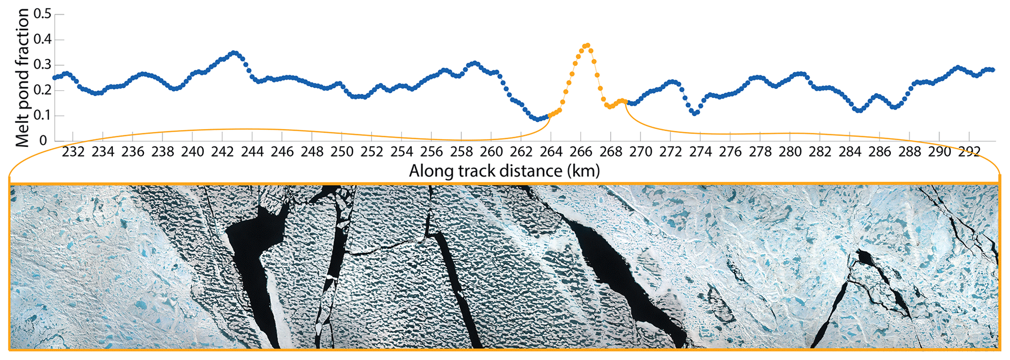
Figure 6Melt pond fraction along a several-kilometer section of the 24 July 2017 flight. The orange highlighted region is depicted as a series of stitched together DMS images that show a first-year inclusion between two multiyear floes.
3.2 Influence of ice type on melt pond fractions
Each summer transect was categorized into first-year ice, multiyear ice, or mixed ice based on manual inspection of those flight's images. The delineation of ice type was based on pond shape, color, and distribution as well as ice surface topography (Johnston and Timco, 2008). The flights classed as a single ice type had at least 90 % (estimated from visual inspection) of that type. Melt pond statistics for single ice type flights are shown as box-and-whisker plots in Fig. 7, where each flight is colored by its ice type categorization: blue for FYI and green for MYI. In these plots the box outline shows the 75th and 25th percentiles, the middle line displays the median, the whiskers show 1.5× the interquartile range, and the red points are outliers. Generally, the 2016 flights departing from Utqiaġvik, Alaska, observed FYI while the 2017 flights departing from Thule AFB, Greenland, observed MYI. There are three exceptions to this categorization: 13 July 2016 and 19 July 2016 contain both ice types, where small pockets of MYI were included in the northern sections of an otherwise primarily FYI region, and flight A on 25 July 2017 covers FYI. Statistics for the two mixed ice type flights are plotted separately in Fig. 8, where each flight is divided into FYI or MYI categories.
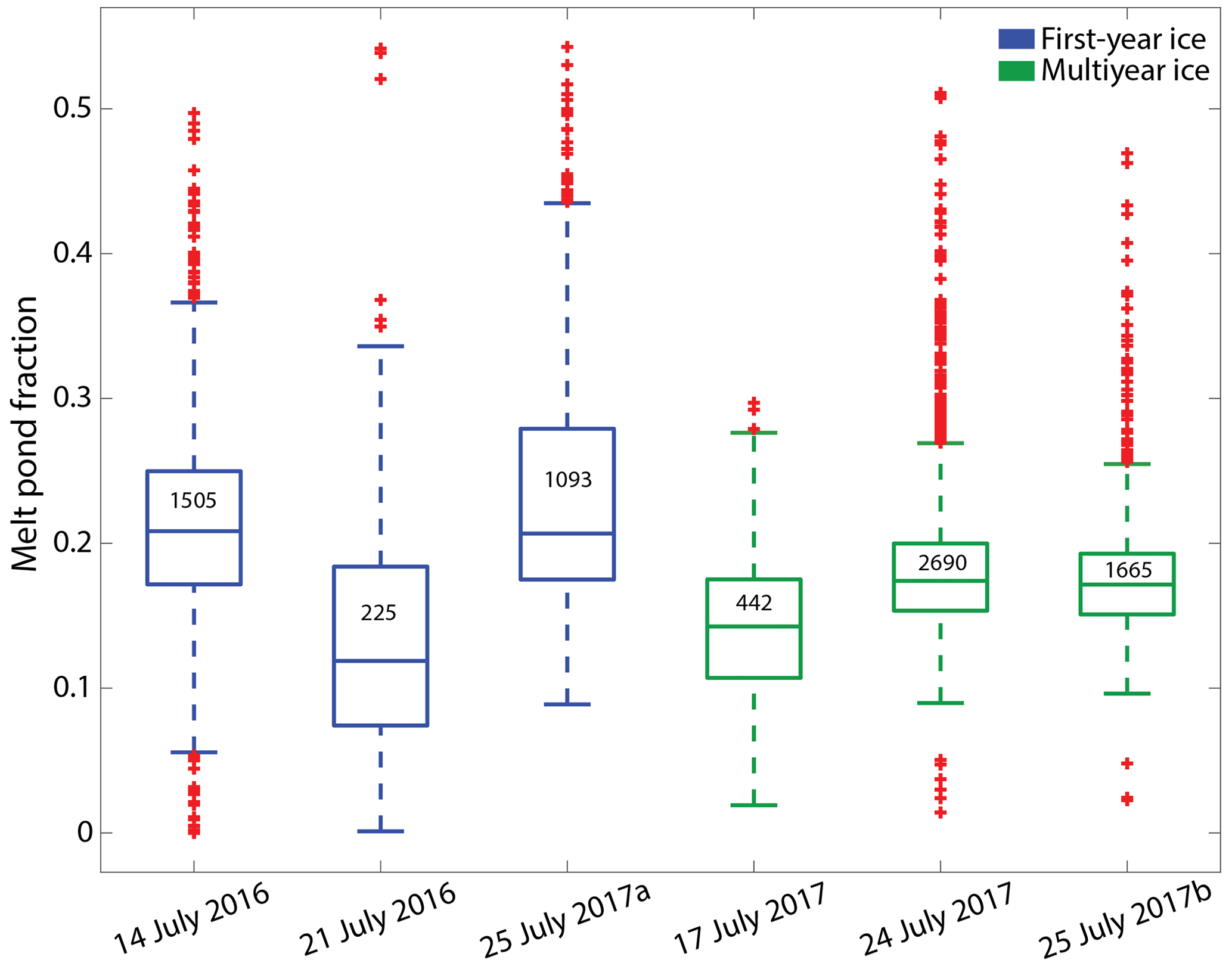
Figure 7Melt pond statistics from summer OIB flight which contained only a single ice type. Blue corresponds to first-year ice statistics, green to multiyear ice statistics, and red crosses indicate outliers. The number of image frames used to calculate statistics for each flight is included inside each box. The approximate area of each image frame is 0.25 km2.
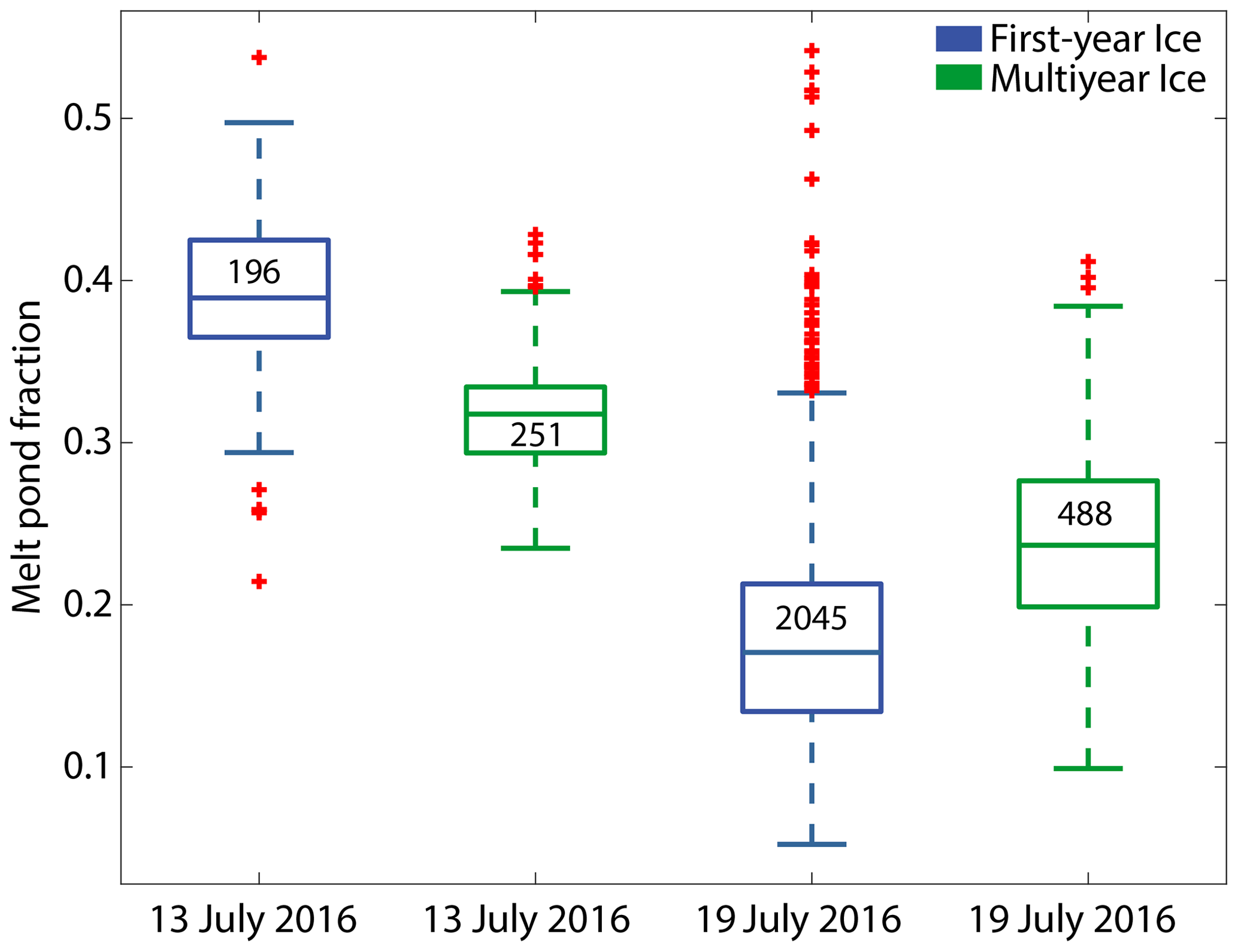
Figure 8Melt pond statistics from two flights that contain both first-year and multiyear ice. In the 13 July 2016 case, multiyear ice has a lower pond fraction, while in the 19 July 2016 case the first-year ice has a lower pond fraction. Blue corresponds to first-year ice statistics, green to multiyear ice statistics, and red crosses indicate outliers. The number of image frames used to calculate statistics for each flight is included inside the box. The approximate area of each image frame is 0.25 km2.
Figure 7 reveals two insights into the difference in melt pond fractions between FYI and MYI. First, there is no obvious difference in the median pond fraction between flights, and second, there is more variance in the pond fractions on FYI. The variance is described by the interquartile range, the mean of which is 0.1 for the first-year flights and 0.05 for the multiyear flights. In other words, while FYI exhibited a wider range of possible pond fractions, the average coverage is not observed to be higher than on MYI. The difference in timing and region between OIB flights precludes drawing general conclusions about differences in median melt pond fraction between ice types. However, two flights that contained both FYI and MYI were selected for further analysis to investigate melt pond statistics across ice that experienced similar forcing conditions: 13 July 2016 and 19 July 2016. The portions of these transects that depict each ice type were manually determined. Results, delineated by ice type, for these two flights are shown in Fig. 8. The key observation here is that the two flights have opposite relationships. On 13 July, the FYI has a higher median pond fraction, while on 19 July, the FYI has a lower median pond fraction. Previous work has shown the possibility for FYI to have lower pond cover than MYI at local scales, i.e., individual floes (Eicken et al., 2004; Webster et al., 2015). Our results support this observation and show that it can also happen at regional scales. That pond coverage is more variable on FYI than it is on MYI suggests that while ponds evolve differently on each type there is not a simple relationship in mean pond fraction. In other words, one cannot conclude that FYI has either higher or lower pond fractions than MYI.
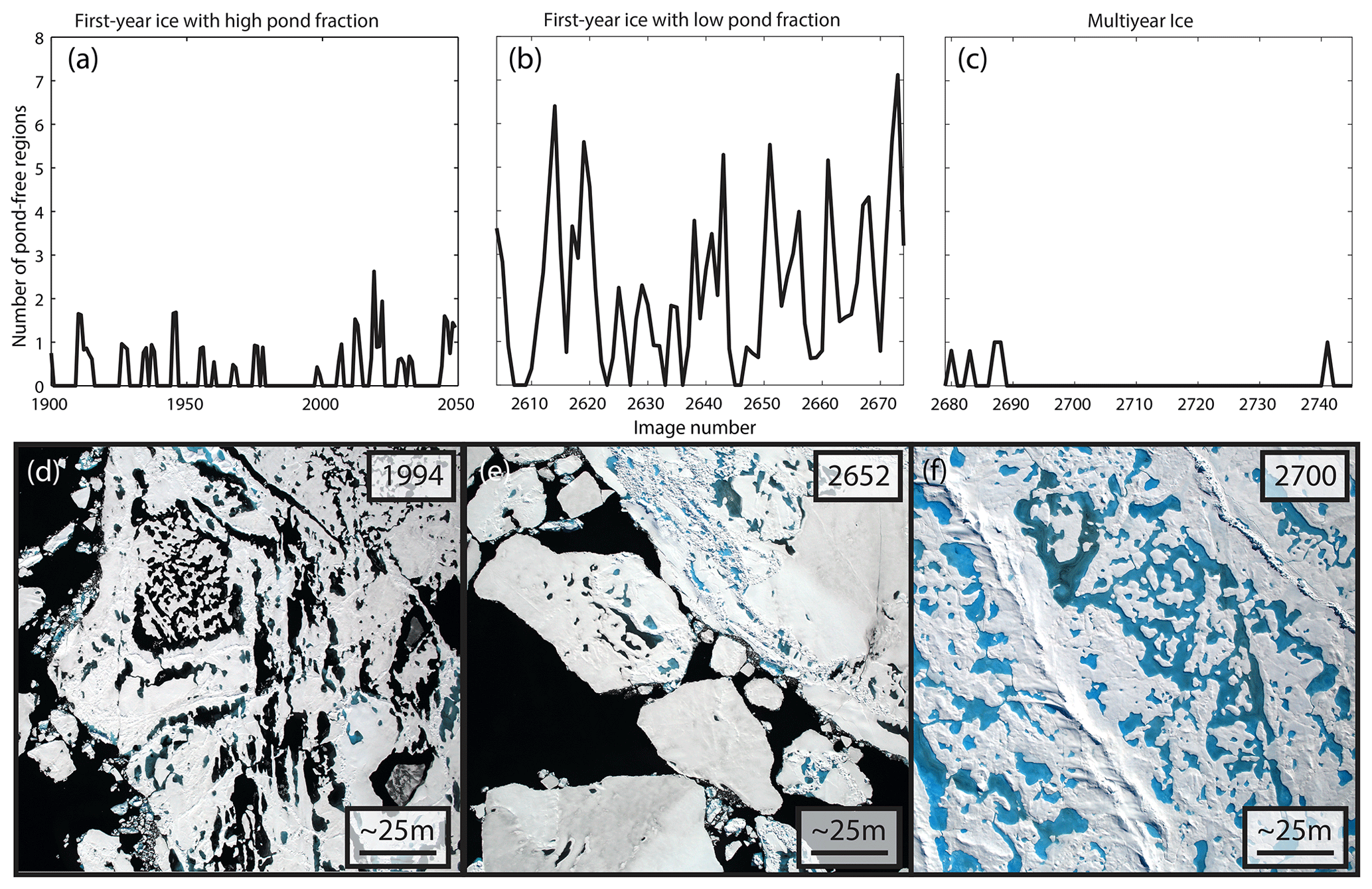
Figure 9Number of pond-free areas detected over several regions of sea ice observed during the 19 July 2016 flight. Panels (d), (e), and (f) show an example image from the regions plotted in panels (a), (b), and (c), respectively.
3.3 Observations of pond-free first-year ice
The frequency at which FYI develops low pond coverage was investigated using the pond-free region detection algorithm to find large unponded areas. Figure 9 shows the results of applying this algorithm to selected segments of the 19 July 2016 flight. Panel (a) shows the results for a portion of primarily FYI with high pond coverage, (b) shows a region of FYI that has many areas of pond-free ice, and (c) shows results from a section of MYI. The ice analyzed for Fig. 9a is what we understand would be considered as a common state for FYI in an advanced state of melt, where ponds have drained to sea level but a high portion of the ice floe remains below freeboard and yields a uniformly high pond fraction. This state coincides with the third stage of pond evolution. This contrasts with the FYI analyzed for Fig. 9b where, while melt ponds are still present, there are large open areas of pond-free ice. The ponds on the MYI floe are regularly distributed and the fractional pond coverage shows little variance. This could coincide with stage 2 of pond evolution, where ponds have drained and none remain above freeboard, or to a region where ponds never formed. A time series would be required to distinguish these paths. Expanding from these regions of this specific flight, 17 % of all summer FYI images processed for this study have three or more large pond-free regions. This reiterates previous observations by Eicken et al. (2004) that estimated 10 % to 30 % of FYI surrounding the SHEBA ice camp had “low or zero pond cover”. In contrast, in the MYI portion of this dataset, only 5 % of images have three or more large pond-free regions. While there is a clear difference between the MYI and FYI types, the important observation here is the large percentage of FYI that has lower-than-expected pond coverage.
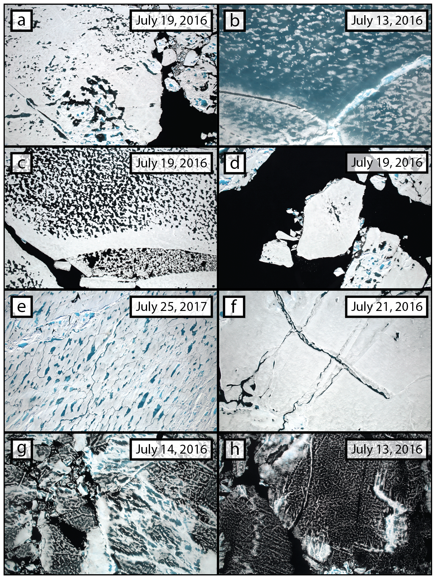
Figure 10Exhibits of sea ice surface features as seen in the DMS dataset. Each panel is a full IceBridge image, and while flight altitude affects image resolution and footprint, each scene is approximately 600 m by 400 m. See text for full description of each frame.
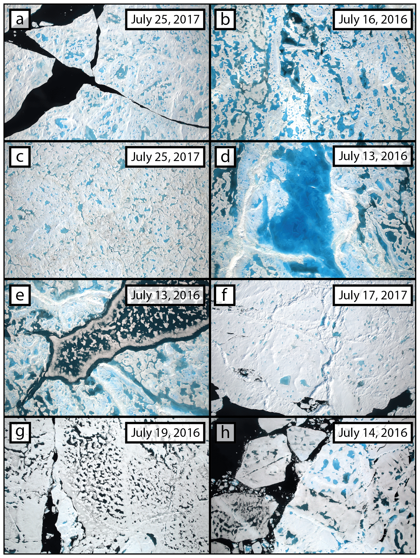
Figure 11Exhibits of sea ice surface features as seen in the DMS dataset. Each panel is a full IceBridge image, and while flight altitude affects image resolution and footprint, each scene is approximately 600 m by 400 m. See text for full description of each frame.
3.4 Snapshots of a summer sea ice cover
In processing the Operation IceBridge optical imagery dataset, we have had the unique opportunity to review a significant library of images detailing different sea ice states, looking at thousands of square kilometers of sea ice. Observations of sea ice on this scale are rare, and notions of what ice states are “typical” or “unusual” are still not well known. In Figs. 10 and 11 we present some examples of what we have observed to be “representative” ice states and examples of ice conditions that are uncommon. The OSSP-analyzed results for each frame in Figs. 10 and 11 are in Figs. S1 and S2 in the Supplement, respectively. These are intended to serve as a qualitative summary of the extensive OIB observations, against which future campaigns can be quickly compared. For each presented image we label the noted features based on the frequency at which we have observed them. Along an arbitrary 100 km transect of ice in a given melt state, common describes a feature that can be expected on more than half of the ice, occasional describes features that would be expected to show up 5–10 times, and infrequent describes a feature that may present once or twice.
Sea ice scenes shown in Fig. 10 are as follows: (a) FYI that shows a wide range of the possible melt pond fractions, ranging from pond-free to high pond coverage; occasional; (b) highly ponded level FYI scene in early melt, where ice appears as islands in a sea of water; such ice was common in large areas in the Chukchi Sea; (c) FYI with high pond fraction and very interconnected pond structure. This is common and it represents the generally understood behavior of FYI. Here we also see that ponds preferentially form towards the middle of the floe, leaving a pond-free border around the edge. The floe-edge gradients are particularly strong in this image; the pond-free border is an occasional feature. (d) Example of a floe where ponds preferentially form away from the edges. These small floes with central ponds were common in broken FYI. (e) Shorefast level ice in the Lincoln Sea. Ponds have started to drain already, as evidenced by the drainage channels visible throughout the ice. This type of relatively low coverage and consolidated ponds were infrequent in the OIB dataset but may be common for ice in this region. We speculate that deep snow dunes and thick ice are responsible. (f) This image shows a region that appears to have had a recent summer snowfall event. The snow serves to fill shallow ponds with slush or to completely cover them and significantly lowers pond fraction – infrequent in the OIB dataset as it is dependent on specific weather conditions. (g) A common example of high pond fraction FYI. (h) Flat and thin ice pans that are almost completely covered by meltwater, this scene is common for late stages of melt on FYI.
Sea ice scenes shown in Fig. 11 are as follows: (a–c) these are common examples of ponded MYI floes with characteristically blue ponds that are well consolidated by surface topography, showing the range of pond fractions that are possible. (d) This is an example of large reservoir-like ponds that were only observed on MYI. These are occasional features on large sections of MYI. (e) This shows MYI with FYI inclusions from ocean that refroze during the last winter; this is common for MYI at lower latitudes and occasional at higher latitudes. In cases of small FYI inclusions in MYI fields like this, the FYI ice that is typically darker has a higher pond coverage. (f) This is an example of low-pond-coverage MYI – this was infrequent in the OIB dataset. (g, h) This is ponded FYI undergoing drainage, where evidence of previous ponds is still visible. The overall image represents common features, but the drainage pattern here is infrequently observed, likely due to its short lifespan.
A common hypothesis in the sea ice community states that FYI has, on average, higher melt pond coverage than MYI. While there is considerable nuance to this statement due to the variability of pond coverage over the temporal domain, it represents a testable hypothesis which our results above did not support. It should be noted that this OIB-derived dataset represents single snapshots in time, and while many melt states were observed, it is impossible to assess complete seasonal averages of melt pond coverage here. There are many factors contributing to areal melt pond coverage differences between FYI and MYI. In the early season, when meltwater sits on impermeable ice above sea level, limited topography causes a similar volume of meltwater to flood larger areas of FYI than it would on rougher MYI. This is supported by observations in early melt stages, which show FYI melt pond coverage in excess of 60 %. Such coverage exceeds that seen on MYI at any time (Landy et al., 2014; Polashenski et al., 2012). However, in stage 2, melt pond fraction on FYI tends to decline faster than on MYI because the meltwater can drain to sea level at a faster rate (Polashenski et al., 2012). In the late season, after ponds have drained to sea level, it has been argued that thinner FYI will have less buoyancy and less ice area above freeboard than MYI. In contrast, on thicker FYI the level surface would have fewer depressions and more buoyancy and therefore more ice area above freeboard (e.g., Fig. 10d). The relative pond fraction between FYI and MYI depends on the time along the melt evolution and the ice physical properties. Over many melt states observed in the complete summer dataset (Figs. 7 and 8), we did not find a statistically significant difference in average pond fraction between FYI and MYI.
An alternate hypothesis about the behavior of FYI ponds emerging in some recent papers is that FYI pond coverage is extremely variable and may have bimodal evolution driven by snow topography and permeability (Perovich, 2002; Polashenski et al., 2017; Popović et al., 2018). FYI ponds may not form at all under certain circumstances if the ice is highly permeable or lacks snow cover (Polashenski et al., 2017, and references therein). Other observations show very high melt pond coverage that persists even after ponds drain to sea level (Polashenski et al., 2015). This divergence of pond behavior raises the possibility of bimodal behavior wherein some FYI would flood extensively and experience more ponding than MYI while other FYI might not pond at all. The image dataset analyzed in this study does not support the bimodal hypothesis but rather supports the idea that FYI pond coverage is much more variable than MYI and exists in all states from low to high pond cover. Several factors could be the cause of the high variability seen in our dataset. For example, diurnal effects can play a large role in the melt pond fraction on FYI by significantly changing surface melt rates on short timescales (Eicken et al., 2004; Hanesiak et al., 1999). Alternatively, if ice and snow topography controls pond fraction after ponds drain (Polashenski et al., 2012), FYI where snow dunes or differential melt creates surface roughness will have a higher pond fraction while ice that is level will be pond-free. As the sea ice topography is highly variable, we would expect corresponding variability in the pond fraction.
Examining the pond coverage in more detail provides evidence that the range of possible melt states is larger on FYI than it is on MYI. In other words, FYI exhibits all possible states between low and high coverage, while the MYI pond fraction typically exists within a small window. Returning to the box plots in Fig. 7, note the larger interquartile range (IQR) of the first-year flights versus the multiyear flights. If we were to accept the traditional hypothesis that all FYI had high pond cover, we would expect the FYI to have a higher median but a similar IQR. However, this is not the case. These observations suggest pond cover on FYI is highly variable, and only in a subset of circumstances does the ice exhibit the expected higher pond fraction. Examples of each behavior have been identified in Fig. 8. The traditional understanding of melt pond evolution on FYI, where flat undeformed ice allows meltwater to spread horizontally and create large areas of pond-covered ice, is often observed on landfast ice or ice attached to a multiyear floe (e.g., Barber and Yackel, 1999; Derksen et al., 1997; Fetterer and Untersteiner, 1998; Uttal et al., 2002). For example, Fig. 6b shows a refrozen lead between two MYI floes, where the pond fraction is significantly higher on the flat FYI than on either of the adjoining MYI floes. Along the 19 July 2016 transect many of the smaller (less than 200 m diameter) freely floating floes of flat FYI exhibited little to no pond cover late in the melt season (as seen in Fig. 10d). We also note many examples of floes that are pond-free along their edges, such as in Fig. 10c, and floes that exhibit nearly complete pond coverage (such as Fig. 10b, g, h). This dataset, therefore, helps establish that no simple relationship between FYI and MYI ponding exists and presents the possibility that the transition to FYI is not causing uniformly higher melt pond fraction, as has been expected. Due to the temporal variability in pond evolution, complete time series datasets are needed to fully analyze the relationship between pond fraction and ice age. Understanding the distribution of pond fraction on basin-wide scales would be key to understanding whether the transition from MYI to FYI has a net increase on pond prevalence. No large-scale, comprehensive observations have been available to resolve the prevalence of such behaviors.
A new dataset quantifying sea ice surface fractions observed in Operation IceBridge DMS imagery has been derived using the recently developed OSSP algorithm. This dataset classifies the surface coverage into four categories. During the melt season these categories are (1) snow or thick ice, (2) dark or thin ice, (3) melt ponds and submerged ice, and (4) open water. For freezing conditions, the categories become (1) snow or thick ice, (2) dark or thin ice, (3) open water, and (4) ridge shadows. The dataset allows for the investigation of sea ice surface type distributions along OIB transects and will support follow-on studies, both by analyzing this dataset in isolation (as demonstrated here) and by combining it with coincident OIB datasets such as ice thickness or ice roughness. This dataset is available at the NSIDC for community use. Future improvements to this dataset should include work towards a more sophisticated haze removal algorithm to apply to the OIB optical images. This will increase accuracy and increase the fraction of images that can be successfully processed.
We have investigated snapshots of melt pond coverage differences between FYI and MYI in the Beaufort Sea and Chukchi Sea region for 2016 and the Lincoln Sea for 2017. Our results support previous findings that FYI can have a lower pond fraction than MYI under similar forcing conditions. While the results presented herein cannot definitively confirm or refute the hypothesis that FYI has higher mean pond fraction than MYI, the high variability in FYI pond fraction over large regions suggests that the general rule of thumb that FYI should have higher ponding than MYI is too simplistic. Furthermore, the finding that FYI exhibits much larger variance over its temporal evolution indicates that there is not one path that defines the typical pond coverage changes. We did not find sufficient evidence that there is a strict duality in FYI pond evolution either, and we suggest future process studies investigate the mechanisms that drive FYI towards high or low pond fraction and specifically note that time series image observations and/or field studies may be necessary to unravel this question. The different evolution pathways that pond development can apparently take on FYI may have large impacts on sea ice modeling efforts, through albedo feedbacks. Furthermore, we suggest combining this new melt pond dataset with data available from the IceBridge Airborne Topographical Mapper to determine the relationship between sea ice topography and melt pond formation.
The OSSP algorithm code is available at Zenodo (https://doi.org/10.5281/zenodo.3551033, Wright and Polashenski, 2019). The pond-free detection algorithm is archived at Zenodo (https://doi.org/10.5281/zenodo.3971014, Wright, 2020). Raw Operation IceBridge DMS imagery is available from the National Snow and Ice Data Center (https://doi.org/10.5067/UMFN22VHGGMH, Dominguez, 2010, updated 2018). OSSP-generated results are also archived at the NSIDC (https://doi.org/10.5067/1LI57H56EB7G, Polashenski et al., 2020).
The supplement related to this article is available online at: https://doi.org/10.5194/tc-14-3523-2020-supplement.
NCW was responsible for writing the original draft, creating the data visualizations, reviewing and editing the manuscript, designing and testing the OSSP software updates, conceptualizing and programming the pond-free detection algorithm, and formally analyzing the OSSP-generated results. CMP was responsible for initiating the study, contributing to writing and editing the manuscript, and contributing to methodology and result analysis. STM was responsible for implementing the OSSP software on NASA's Pleiades system, monitoring data processing, and data archiving. RAB was responsible for funding acquisition and supervision for the Ames Research Center team and for review and editing of the manuscript draft.
The authors declare that they have no conflict of interest.
The image processing for this work was carried out on NASA's Advanced Supercomputing Pleiades system. The authors would like to thank the two anonymous reviewers, the community members, and the handling editor for their suggestions which helped improve this publication.
This research has been supported by the NASA AIST Program.
This paper was edited by Petra Heil and reviewed by two anonymous referees.
Barber, D. G. and Yackel, J.: The physical, radiative and microwave scattering characteristics of melt ponds on Arctic landfast sea ice, Int. J. Remote Sens., 20, 2069–2090, https://doi.org/10.1080/014311699212353, 1999.
Bliss, A. C. and Anderson, M. R.: Snowmelt onset over Arctic sea ice from passive microwave satellite data: 1979–2012, The Cryosphere, 8, 2089–2100, https://doi.org/10.5194/tc-8-2089-2014, 2014.
Curry, J. A., Schramm, J. L., and Ebert, E. E.: Sea ice-albedo climate feedback mechanism, J. Climate, 8, 240–247, https://doi.org/10.1175/1520-0442(1995)008<0240:SIACFM>2.0.CO;2, 1995.
De, K. and Masilamani, V.: Image Sharpness Measure for Blurred Images in Frequency Domain, Procedia Engineer., 64, 149–158, https://doi.org/10.1016/J.PROENG.2013.09.086, 2013.
Derksen, C., Piwowar, J., and LeDrew, E.: Sea-Ice Melt-Pond Fraction as Determined from Low Level Aerial Photographs, Arct. Alp. Res., 29, 345–351, https://doi.org/10.1080/00040851.1997.12003254, 1997.
Dominguez, R.: IceBridge DMS L0 Raw Imagery, Version 1, Boulder, Colorado USA. NASA National Snow and Ice Data Center Distributed Active Archive Center, https://doi.org/10.5067/UMFN22VHGGMH, 2010, updated 2018.
Eicken, H., Krouse, H. R., Kadko, D., and Perovich, D. K.: Tracer studies of pathways and rates of meltwater transport through Arctic summer sea ice, J. Geophys. Res.-Oceans, 107, 8046, https://doi.org/10.1029/2000JC000583, 2002.
Eicken, H., Grenfell, T. C., Perovich, D. K., Richter‐Menge, J. A., and Frey, K.: Hydraulic controls of summer Arctic pack ice albedo, J. Geophys. Res.-Oceans, 109, C08007, https://doi.org/10.1029/2003JC001989, 2004.
Fetterer, F. and Untersteiner, N.: Observations of melt ponds on Arctic sea ice, J. Geophys. Res.-Oceans, 103, 24821–24835, https://doi.org/10.1029/98JC02034, 1998.
Hanesiak, J. M., Barber, D. G., and Flato, G. M.: Role of diurnal processes in the seasonal evolution of sea ice and its snow cover, J. Geophys. Res.-Oceans, 104, 13593–13603, https://doi.org/10.1029/1999JC900054, 1999.
Huang, W., Lu, P., Lei, R., Xie, H., and Li, Z.: Melt pond distribution and geometry in high Arctic sea ice derived from aerial investigations, Ann. Glaciol., 57, 105–118, https://doi.org/10.1017/aog.2016.30, 2016.
Hunke, E. C., Hebert, D. A., and Lecomte, O.: Level-ice melt ponds in the Los Alamos sea ice model, CICE, Ocean Model., 71, 26–42, https://doi.org/10.1016/j.ocemod.2012.11.008, 2013.
Johnston, M. E., and Timco, G. W.: Understanding and identifying old ice in summer, Can. Hydraul. Cent., Natl. Res. Counc. Can., Ottawa, 2008.
Landy, J., Ehn, J., Shields, M., and Barber, D.: Surface and melt pond evolution on landfast first-year sea ice in the Canadian Arctic Archipelago, J. Geophys. Res.-Oceans, 119, 3054–3075, https://doi.org/10.1002/2013JC009617, 2014.
Miao, X., Xie, H., Ackley, S., Perovich, D., and Ke, C.: Object-based detection of Arctic sea ice and melt ponds using high spatial resolution aerial photographs, Cold Reg. Sci. Technol., 119, 211–222, https://doi.org/10.1016/j.coldregions.2015.06.014, 2015.
Morassutti, M. P. and Ledrew, B. F.: Albedo and depth of melt ponds on sea-ice, Int. J. Climatol., 16, 817–838, https://doi.org/10.1002/(SICI)1097-0088(199607)16:7<817::AID-JOC44>3.0.CO;2-5, 1996.
Perovich, D. K.: Aerial observations of the evolution of ice surface conditions during summer, J. Geophys. Res.-Oceans, 107, 8048, https://doi.org/10.1029/2000JC000449, 2002.
Perovich, D. and Polashenski, C.: Albedo evolution of seasonal Arctic sea ice, Geophys. Res. Lett., 39, L08501, https://doi.org/10.1029/2012GL051432, 2012.
Perovich, D., Grenfell, T., Richter-Menge, J., Light, B., Tucker, W., and Eicken, H.: Thin and thinner: Sea ice mass balance measurements during SHEBA, J. Geophys. Res.-Oceans, 108, https://doi.org/10.1029/2001JC001079, 2003.
Polashenski, C., Perovich, D., and Courville, Z.: The mechanisms of sea ice melt pond formation and evolution, J. Geophys. Res.-Oceans, 117, C01001, https://doi.org/10.1029/2011JC007231, 2012.
Polashenski, C., Perovich, D. K., Frey, K. E., Cooper, L. W., Logvinova, C. I., Dadic, R., Light, B., Kelly, H. P., Trusel, L. D., and Webster, M.: Physical and morphological properties of sea ice in the Chukchi and Beaufort Seas during the 2010 and 2011 NASA ICESCAPE missions, Deep-Sea Res. Pt. II, 118, 7–17, https://doi.org/10.1016/J.DSR2.2015.04.006, 2015.
Polashenski, C., Wright, N., and McMichael, S.: IceBridge-Related DMS-Derived L4 Sea Ice Surface Cover Classification Orthorectified Images, Version 1, Boulder, Colorado USA, NASA National Snow and Ice Data Center Distributed Active Archive Center, https://doi.org/10.5067/1LI57H56EB7G, 2020.
Polashenski, C., Golden, K., Perovich, D., Skyllingstad, E., Arnsten, A., Stwertka, C., and Wright, N.: Percolation blockage: A process that enables melt pond formation on first year Arctic sea ice, J. Geophys. Res.-Oceans, 122, 413–440, https://doi.org/10.1002/2016JC011994, 2017.
Popović, P., Cael, B. B., Silber, M., and Abbot, D. S.: Simple Rules Govern the Patterns of Arctic Sea Ice Melt Ponds, Phys. Rev. Lett., 120, 148701, https://doi.org/10.1103/PhysRevLett.120.148701, 2018.
Serreze, M. C., Barrett, A. P., Stroeve, J. C., Kindig, D. N., and Holland, M. M.: The emergence of surface-based Arctic amplification, The Cryosphere, 3, 11–19, https://doi.org/10.5194/tc-3-11-2009, 2009.
Stroeve, J. C., Serreze, M. C., Holland, M. M., Kay, J. E., Malanik, J., and Barrett, A. P.: The Arctic's rapidly shrinking sea ice cover: a research synthesis, Clim. Change, 110, 1005–1027, https://doi.org/10.1007/s10584-011-0101-1, 2012.
Uttal, T., Curry, J. A., Mcphee, M. G., Perovich, D. K., Moritz, R. E., Maslanik, J. A., Guest, P. S., Stern, H. L., Moore, J. A., Turenne, R., Heiberg, A., Serreze, M. C., Wylie, D. P., Persson, O. G., Paulson, C. A., Halle, C., Morison, J. H., Wheeler, P. A., Makshtas, A., Welch, H., Shupe, M. D., Intrieri, J. M., Stamnes, K., Lindsey, R. W., Pinkel, R., Pegau, W. S., Stanton, T. P., Grenfeld, T. C., Uttal, T., Curry, J. A., Mcphee, M. G., Perovich, D. K., Moritz, R. E., Maslanik, J. A., Guest, P. S., Stern, H. L., Moore, J. A., Turenne, R., Heiberg, A., Serreze, M. C., Wylie, D. P., Persson, O. G., Paulson, C. A., Halle, C., Morison, J. H., Wheeler, P. A., Makshtas, A., Welch, H., Shupe, M. D., Intrieri, J. M., Stamnes, K., Lindsey, R. W., Pinkel, R., Pegau, W. S., Stanton, T. P., and Grenfeld, T. C.: Surface Heat Budget of the Arctic Ocean, B. Am. Meteorol. Soc., 83, 255–275, https://doi.org/10.1175/1520-0477(2002)083<0255:SHBOTA>2.3.CO;2, 2002.
van der Walt, S., Schönberger, J. L., Nunez-Iglesias, J., Boulogne, F., Warner, J. D., Yager, N., Gouillart, E., and Yu, T.: scikit-image: image processing in Python, PeerJ, 2, e453, https://doi.org/10.7717/peerj.453, 2014.
Webster, M. A., Rigor, I. G., Perovich, D. K., Richter-menge, J. A., Polashenski, C. M., and Light, B.: Seasonal evolution of melt ponds on Arctic sea ice, J. Geophys. Res.-Oceans, 120, 1–15, https://doi.org/10.1002/2015JC011030, 2015.
Wright, N.: wrightni/pondfree_detection: v1.0 (Version v1.0), Zenodo, https://doi.org/10.5281/zenodo.3971014, 2020.
Wright, N. C. and Polashenski, C. M.: Open-source algorithm for detecting sea ice surface features in high-resolution optical imagery, The Cryosphere, 12, 1307–1329, https://doi.org/10.5194/tc-12-1307-2018, 2018.
Wright, N. and Polashenski, C.: Open Source Sea-ice Processing Algorithm v2.3 (Version v2.3), Zenodo, https://doi.org/10.5281/zenodo.3551033, 2019.