On the importance of snowpack stability, the frequency distribution of snowpack stability, and avalanche size in assessing the avalanche danger level

Consistency in assigning an avalanche danger level when forecasting or locally assessing avalanche hazard is essential but challenging to achieve, as relevant information is often scarce and must be interpreted in light of uncertainties. Furthermore, the definitions of the danger levels, an ordinal variable, are vague and leave room for interpretation. Decision tools developed to assist in assigning a danger level are primarily experience-based due to a lack of data. Here, we address this lack of quantitative evidence by exploring a large data set of stability tests (N=9310) and avalanche observations (N=39 017) from two countries related to the three key factors that characterize avalanche danger: snowpack stability, the frequency distribution of snowpack stability, and avalanche size. We show that the frequency of the most unstable locations increases with increasing danger level. However, a similarly clear relation between avalanche size and danger level was not found. Only for the higher danger levels did the size of the largest avalanche per day and warning region increase. Furthermore, we derive stability distributions typical for the danger levels 1-Low to 4-High using four stability classes (very poor, poor, fair, and good) and define frequency classes describing the frequency of the most unstable locations (none or nearly none, a few, several, and many). Combining snowpack stability, the frequency of stability classes and avalanche size in a simulation experiment, typical descriptions for the four danger levels are obtained. Finally, using the simulated stability distributions together with the largest avalanche size in a stepwise approach, we present a data-driven look-up table for avalanche danger assessment. Our findings may aid in refining the definitions of the avalanche danger scale and in fostering its consistent usage.

1 Introduction

Consistent communication of regional avalanche hazard in publicly available avalanche forecast products is paramount for avoiding misinterpretations by the users (Techel et al., 2018). A key piece of information in public bulletins is the avalanche danger level. The danger levels – from 1-Low to 5-Very High – are described in the European Avalanche Danger Scale (EADS; EAWS, 2018) or its North American equivalent, the North American Avalanche Danger Scale (e.g., Statham et al., 2010) with brief definitions of the key factors. The key factors that characterize avalanche danger are as follows (Meister, 1995; EAWS, 2020, 2018):

• the probability of avalanche release,

• the frequency and location of the triggering spots, and

• the expected avalanche size.

These elements are expected to increase with increasing danger level (e.g., Schweizer et al., 2020).

The probability of avalanche release, or “sensitivity to triggers” as termed in the Conceptual Model of Avalanche Hazard (CMAH; Statham et al., 2018a), is inversely related to snowpack stability, with a higher probability of an avalanche releasing with lower stability and vice versa (e.g., Föhn and Schweizer, 1995; Meister, 1995). Hence, the probability of avalanche release refers to a specific location and relates to the local (or point) snow instability. The latter has recently been revisited, and three elements were suggested for describing point snow instability: failure initiation, crack propagation, and slab tensile support (Reuter and Schweizer, 2018).

The frequency and location of the triggering spots is typically unknown. So far, it can only be assessed with laborious extensive sampling (e.g., Birkeland, 2001; Reuter et al., 2016). However, in a regional avalanche forecast the spatial distribution of snow instability can be described with regard to the frequency and the locations of triggering spots or more generally the locations where snowpack stability is lowest. Of these two components, frequency and location, only frequency is relevant when assessing the danger level (Schweizer et al., 2020). The frequency always refers to a specific area, typically a forecast region and/or slope aspects and elevation bands. The frequency distribution describes the question, “how often do spots with a certain snowpack stability exist within a region?” – in terms of numbers, proportions, or percentages. Typical frequency distributions for the danger levels 1-Low to 3-Considerable were described by Schweizer et al. (2003) using five classes of snowpack stability. Frequency expresses the number of triggering locations assuming a uniform distribution within the reference area and is described using the terms single, some, many, and most (EAWS, 2017). In contrast, the location of triggering spots or of snowpack stability refers to the question, where in the terrain is avalanche release most likely? It indicates where in the terrain the frequency is slightly higher (e.g., where the snowpack is shallow, close to ridgelines, or in bowls). In the CMAH (Statham et al., 2018a), on the other hand, the spatial distribution is related to the spatial density and distribution of an avalanche problem and the ease of finding evidence for it and is described using the three terms isolated, specific, and widespread.

Finally, avalanche size is defined with sizes ranging from 1 to 5 relating to the destructive potential of an avalanche (e.g., CAA, 2014; EAWS, 2019; McClung and Schaerer, 1981).

The EADS descriptions of the key factors for each of the five categories of danger level leave ample room for interpretation and are even partly ambiguous. This may be a major reason for inconsistencies noted in the use of the danger levels among individual forecasters or field observers and, even more prominently, among different forecast centers and avalanche warning services (Lazar et al., 2016; Statham et al., 2018b; Techel and Schweizer, 2017; Techel et al., 2018), which is also a factor when assessing different avalanche problems (Clark, 2019).

The same danger level can be described with different combinations of the three factors. To improve consistency in the use of the danger levels, a first decision aid, the Bavarian Matrix was adopted by the European Avalanche Warning Services (EAWS) in 2005. The Bavarian Matrix, a look-up table, combined the frequency of triggering locations with the release probability. In 2017, an update of the Bavarian Matrix, now called the EAWS Matrix, was presented that additionally incorporates avalanche size (EAWS, 2020). More recently, a so-called Avalanche Danger Assessment Matrix (ADAM; Müller et al., 2016) was proposed, which tries to combine the workflow described in the CMAH with the assignment of the danger levels based on the three factors as suggested in the EAWS Matrix. Both the current version of the EAWS Matrix and ADAM are works in progress.

Challenges in the improvement of these decision support tools include the fact that the three key factors characterizing avalanche danger are not clearly defined and hence are poorly quantified (Schweizer et al., 2020). Our objective is therefore to address this lack of quantitative evidence by exploring observational data relating to snowpack stability, its frequency distribution, and avalanche size. The data originate from different snow climates and also from different avalanche warning services (Norway, Switzerland). The key questions are (1) how do the three factors relate to the danger levels? and (2) which combination of the actual value of the three factors best describes the various danger levels? We present a methodology to generate data-driven stability distributions and to obtain class intervals describing the frequency of a given snowpack stability class. Finally, we will compare the findings with currently used definitions in avalanche forecasting, such as EADS and CMAH, and make recommendations for improvements towards more consistent usage of the danger scale.

2 Data

All the data described below were recorded for the purpose of operational avalanche forecasting in Norway (NOR; Norwegian Water Resources and Energy Directorate NVE) or Switzerland (SWI; WSL Institute for Snow and Avalanche Research SLF). In the vast majority of cases, these observations were provided by specifically trained observers, belonging to the observer network of either the Norwegian or the Swiss avalanche warning service.

For the analysis, we rely primarily on the Swiss data, using the Norwegian data for comparison and validation. Nevertheless, we will occasionally present results for Swiss and Norwegian data side by side.

2.1 Avalanche danger level

The avalanche danger level is an estimate at best, as there is no straightforward operational verification. Whether assessing the danger level in the field or in hindsight, it remains an expert assessment (Föhn and Schweizer, 1995; Techel and Schweizer, 2017).

We rely on the local danger level estimate provided by specifically trained observers. In both countries, this estimate is based on the observations made on the day and on other information considered relevant (Kosberg et al., 2013; Techel and Schweizer, 2017) and can be called a local nowcast. In very few exceptions (19 d during the verification campaigns in the winters 2002 and 2003 in the region surrounding Davos, SWI) was a “verified” regional danger rating available (Schweizer et al., 2003; Schweizer, 2007b).

In this study, we make use of local estimates for dry-snow conditions only. Each stability test or avalanche observation was linked to a danger rating as described below (Sect. 2.2 and 2.3).

Table 1 Data overview.

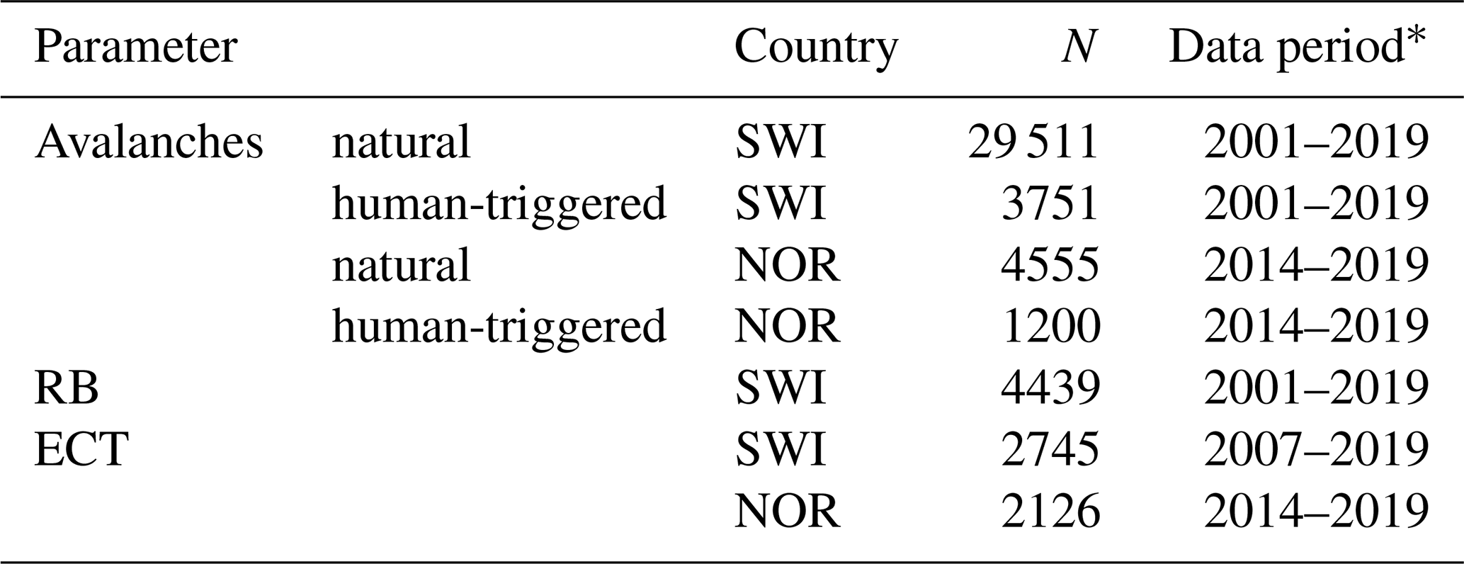
^* For days between (and including) 1 December and 30 April.

2.2 Snowpack stability

Operationally available information directly related to snow instability includes simple field observations as well as snowpack stability tests (Schweizer and Jamieson, 2010). Field observations such as recent avalanching, shooting cracks, and whumpfs (a sound audible when a weak layer fails due to localized loading) clearly indicate snow instability (Jamieson et al., 2009; Schweizer and Jamieson, 2010). These observations are often made in the backcountry while ski touring and do not require a person to dig a snow pit. Snowpack stability tests, on the other hand, are considered targeted sampling (McClung and Schaerer, 2006) with the aim to assess point snow instability. Here, we used data obtained with two stability tests regularly used to assess snow instability in Switzerland and Norway, the rutschblock test and the extended column test.

The rutschblock (RB) test is a stability test, ideally performed on slopes steeper than 30^∘, where a 1.5 m×2 m block of snow is isolated from the surrounding snowpack and loaded by a person (e.g., Föhn, 1987; Schweizer, 2002). An observer performing an RB test records which of the six loading steps, referred to as the score, caused failure and what portion of the block slid (the release type – whole block, most of block, edge only). If no failure occurs, RB7 is recorded. The score and release type provide information on failure initiation and crack propagation, essential components of slab avalanche release (Schweizer et al., 2008b). RB data were only available from Switzerland.

The extended column test (ECT) is a stability test that provides an indication of crack propagation propensity (Simenhois and Birkeland, 2006, 2009). In contrast to the RB test, the ECT is performed on a relatively small (30 cm×90 cm) isolated column of snow and loaded by tapping on the block. The observer records the tap at which a crack initiates (1–30) and whether a fracture propagates across the entire column (ECTP) or not (ECTN; Simenhois and Birkeland, 2009). If no fracture is initiated with 30 taps ECTX is recorded.

Each stability test was linked to a danger rating relating to dry-snow conditions. We considered the danger rating, which was transmitted together with the snow profile or stability test (in text form, SWI), most relevant. In the Swiss data set, this danger rating was replaced for stability tests observed on days and in warning regions for which a verified regional danger rating existed (Sect. 2.1). If neither of them was available, the operational database was searched for local danger level estimates reported during the day and in the same region. Often, these local estimates were reported by the same observer who performed the test.

The Swiss RB data set comprised 4439 RBs, observed mainly on NW-, N-, and NE-facing slopes (67 %) at a median elevation of 2380 m a.s.l. (interquartile range IQR 2160–2565 m) and a median slope angle of 35^∘ (IQR 32–37^∘). The Swiss ECT data set contained 2745 ECTs; 67 % were observed on NW-, N-, and NE-facing slopes at a median elevation of 2372 m a.s.l. (IQR 2134–2547 m) and at 34^∘ (IQR 31–36^∘). The Norwegian ECT data set consisted of 2126 ECTs, observed at a median elevation of 760 m a.s.l. (IQR 730–1067 m). Consistent information on the slope aspect was not available for Norwegian stability data.

2.3 Avalanches

As part of the daily observations, observers (and occasionally the public) reported avalanches observed in their region. Avalanches can be reported not only individually but also by summarizing several avalanches into one observation. While individual avalanches were reported in a similar way in SWI and NOR, the reporting of several avalanches differed. In SWI, observers reported the number of avalanches of a given size. In all reporting forms, information about the wetness and trigger type could be provided. In NOR, observers reported avalanche size, trigger type, and wetness, which was typical for the situation, and described the observed number of avalanches using categorical terms (single 1, some 2–4, many 5–10, numerous ≥11). In both countries, avalanche size was estimated according to the destructive potential and a combination of total length and volume, resulting in avalanche sizes of 1 to 5 (EAWS, 2019). In SWI until 2011, only size classes 1–4 were used.

The analysis was restricted to dry-snow avalanches, where the trigger type was either natural release or human-triggered. These avalanches were linked to a dry-snow local danger rating for the release date of the avalanche(s) in the same warning region.

To enhance the quality of the data, we filtered observations that we believe may indicate errors in the local estimate of the danger level or of avalanche size. To this end, we calculated the avalanche activity index (AAI; Schweizer et al., 1998), a dimensionless index summing up avalanches according to their size with weights of 0.01, 0.1, 1, and 10 for avalanche sizes 1 to 4, respectively. We did not assign weights to the trigger type (natural, human-triggered). For NOR, where the number of observed avalanches is described categorically, we assigned numbers as follows: one =1, few (2–5) =3, several (6–10) =8, and numerous (≥11) =12. For each country, we then rank-ordered the avalanche data and the lowest 2.5 % of the days and regions with 2-Moderate, 3-Considerable, and 4-High, and the top 2.5 % of the days and regions with 1-Low, 2-Moderate, or 3-Considerable were considered to represent errors in the local estimate of the danger level or of avalanche size. These potentially erroneous data were removed.

The total number of avalanches that remained was 33 262 in Switzerland, representing 6610 cases (different days and/or different warning regions), and 5755 in Norway (1618 cases; Table 1).

3 Methods

3.1 Classification of snowpack stability

Snowpack stability is one of the three contributing factors of avalanche hazard and relates to the probability of avalanche release. In the following, we describe how we classified the results of the snow instability tests into the four stability classes (very poor, poor, fair, and good).

Rutschblock (RB) test results were classified into the four stability classes according to Fig. 1a using a combination of score and release type, which have been shown to be good predictors of unstable conditions (e.g., Föhn, 1987; Jamieson and Johnston, 1995; Schweizer et al., 2008b). This stability rating is close to the operationally applied stability rating in Switzerland, which includes five classes and in addition considers weak-layer properties and snowpack structure (Schweizer, 2007a; Schweizer and Wiesinger, 2001). The classification by Schweizer (2007a) was used in Techel and Pielmeier (2014) for an automatic assignment of stability based on RB score and release type (also five classes). As in Techel et al. (2020), we combined the two classes very good and good into one class called good.

Extended column test (ECT) results were classified relying on the classification recently suggested by Techel et al. (2020). Using a combination of crack propagation and the number of taps until failure initiation, four stability classes were defined (Fig. 1b). As the four stability classes for the RB test and ECT do not exactly line up, we assigned the following four class labels to the four ECT classes: poor, poor-to-fair, fair, and good (as in Techel et al., 2020).

If failures in several weak layers were induced in a single stability test, the test results were classified for each failure layer. For this, we considered the failure as not relevant (rating the test result as good) if a failure layer was less than 10 cm below the snow surface (as in Techel et al., 2020). The lowest stability class was retained for further analysis.

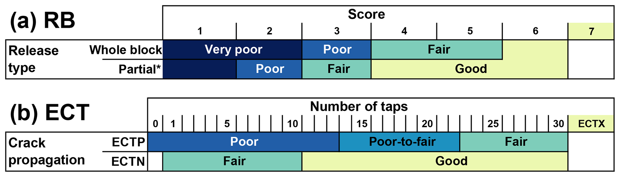
Figure 1 Stability classification of (a) rutschblock test results (based on Schweizer, 2007a; Techel and Pielmeier, 2014) and (b) extended column test results (based on Techel et al., 2020). ^* Partial includes release types most of block and edge only.

3.2 Simulation of snowpack stability distributions

The second factor contributing to avalanche hazard is the frequency of potential triggering locations or of snowpack stability.

To determine the frequency distribution of point snow instability within a defined region and at a given danger level many stability test results on a given day are in general needed (e.g., Schweizer et al., 2003). However, as we most often only had one stability test result on a given day, we followed an alternative approach. Assuming that a single test result is just one sample from the stability distribution on that day and that different days with the same danger level exhibit a range of similar stability distributions, we generated stability distributions by random sampling from the entire population of stability tests at a given danger level. Thus, we applied bootstrap sampling (Efron, 1979) and proceeded as follows (see also Fig. 2a and b):

• i.

  We randomly selected n stability test results with replacement from the stability tests associated with the same danger level, resulting in a single bootstrap sample. We repeated this procedure B times for each danger level.

• ii.

  For each of the B bootstrap samples, we calculated the proportions of very poor, poor, fair, and good stability tests.

Bootstrap sampling, frequently used to estimate the accuracy of a desired statistic or for machine learning (Hastie et al., 2009), requires a sufficiently large number of replications B to be drawn. We used B=2500 for each danger level, resulting in 10 000 stability distributions in total.

The second important parameter when bootstrap sampling is the number n of stability tests drawn in each sample. Small values of n increase variance and hence overlap between samples drawn from different danger levels and reduce the resolution of the desired statistic (e.g., for n=10, the resolution is 0.1; for n=100 it is 0.01). Since nature is not as discrete as the danger levels suggest, we wanted both some overlap between our sampled stability distributions and a reasonably high resolution of our statistic. Unfortunately, there are no studies we can refer to concerning the amount of overlap that would be appropriate. We tested $n=\mathit{\{}\mathrm{10},\mathrm{25},\mathrm{50},\mathrm{100},\mathrm{200},\mathrm{1000}\mathit{\}}$.

These simulations are compared to a small number of days when more than six RB tests (N=41) or more than six ECTs (N=31) were collected in the surroundings of Davos (Switzerland).

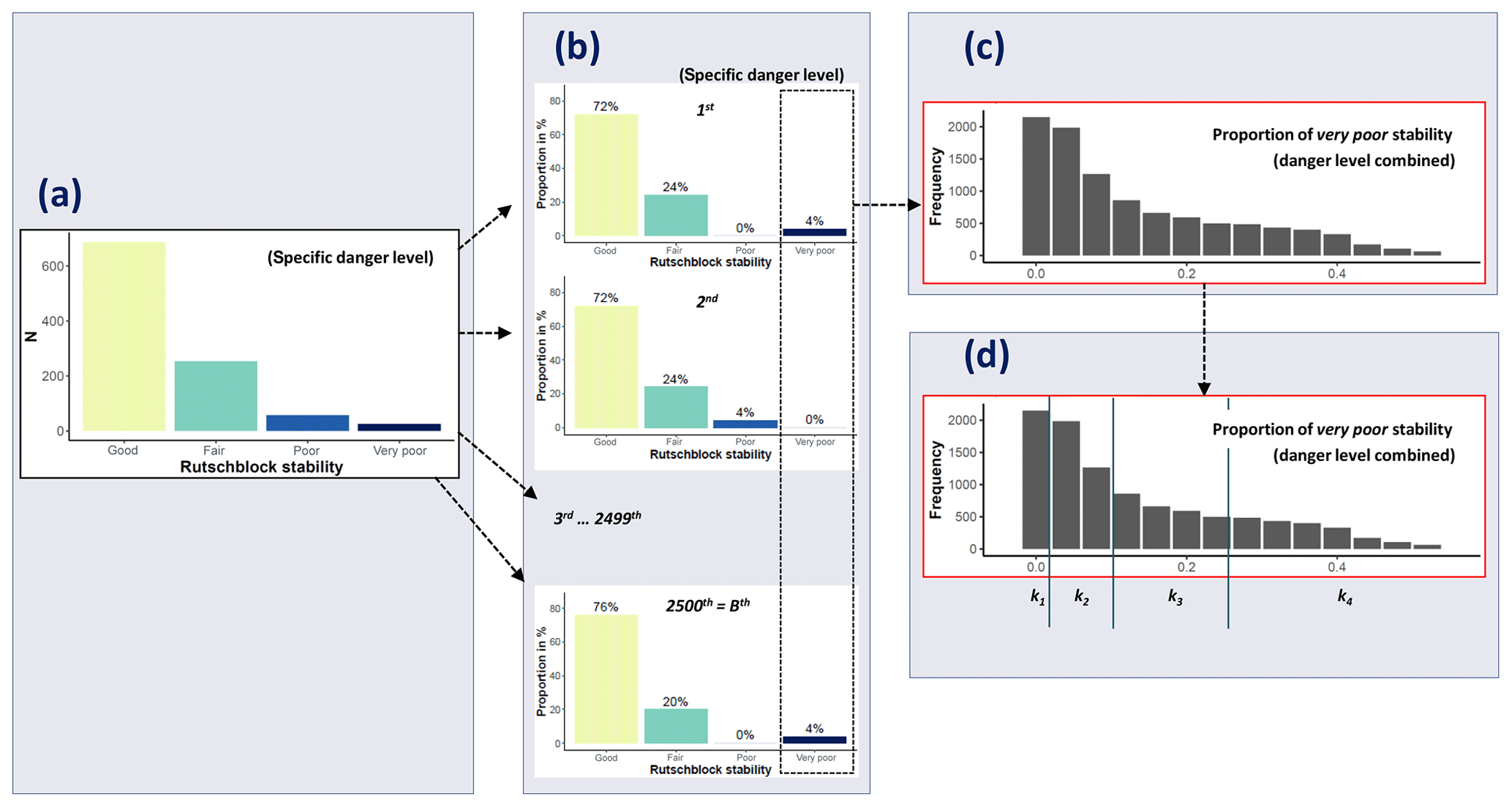
Figure 2 Schematic representation of the workflow for bootstrap sampling and frequency class definition. (a) For each danger level, all stability ratings are combined. (b) From the observed stability distributions of a specific danger level (a), n tests are randomly sampled. This is repeated B=2500 times to obtain typical stability distributions for each of the four danger levels. (c) The 4×2500 bootstrap samples are merged, and the proportion of very-poor-rated stability tests per sample is plotted as a histogram, irrespective of danger level. (d) The statistics required for frequency class definitions are calculated, and the k frequency classes defined. For details refer to the description in Sect. 3.2 and 3.3.

3.3 Snowpack stability and the frequency distribution of snowpack stability – approach to define frequency classes

Currently, neither well-defined terms to describe frequency classes (such as a few or many) nor thresholds to differentiate between the classes exist. In the following, we therefore introduce a data-driven approach to define class intervals that we will use to describe the frequency of a certain snowpack stability class. We considered the following points:

• Classes should be defined based on the snowpack stability class most relevant with regard to avalanche release, hence the frequency of the class very poor. Even though the focus is on the proportion of very poor snowpack stability, classes need to capture the entire possible parameter space, i.e., from very rare to virtually all (1 % to 99 %).

• The number of classes should reflect the human capacity to distinguish between them. We explored three, four, and five classes only, as these are the number of classes currently used to describe and communicate avalanche hazard and its components (e.g., three spatial distribution categories in the CMAH, four frequency terms in the EAWS Matrix, five danger levels, five avalanche size classes).

• Classes must be sufficiently different to ease classification by the forecaster as well as communication to the user. And, if quantifier terms were assigned to these classes, these terms would need to unambiguously describe such increasing frequencies. An example of such a succession of five terms is nearly none, a few, several, many, and nearly all (e.g., Díaz-Hermida and Bugarín, 2010).

Data-driven approaches for defining interval classes are numerous and are described for instance for thematic mapping (e.g., Slocum et al., 2005) or for selecting histogram bin widths (e.g., Evans, 1977; Wand, 1997). In general, the choice of class intervals should be appropriate to the observed data distribution. Approaches include, among others, splitting the parameter space into equal intervals, splitting the parameter space into intervals with an equal number of observations in each bin, or finding natural breaks in the data by minimizing the within-class variance while maximizing the distance between the class centers (e.g., Fisher–Jenks algorithm; Slocum et al., 2005). However, in our case, in which low values of the proportion of very poor stability are frequent and higher values rare, we made use of a geometric progression of class widths considered most suitable for this type of distribution (Evans, 1977). Using this approach, we classified the data into k classes with class interval limits being {0, a, ab, ab², …, ab^k−1, 100}, where a is the size (width) of the initial (lowest) class and b is a multiplying factor. According to Evans (1977), a data-driven calculation of b for the closed interval from 0 to 100 can be given:

$$\begin{array}{}\text{(1)}& b={\left({\displaystyle \frac{\mathrm{100}-{\mathrm{VP}}_{\mathrm{med}}}{{\mathrm{VP}}_{\mathrm{med}}}}\right)}^{\frac{\mathrm{2}}{k}},\end{array}$$

where VP_med (0–100) is the median proportion of very poor stability and k the number of classes preferred. This approach requires a suitable value of the number of classes k to be defined. Given k and b, the initial class width a is (Evans, 1977)

$$\begin{array}{}\text{(2)}& a={\displaystyle \frac{{\mathrm{VP}}_{\mathrm{med}}(\mathrm{100}-b)}{\mathrm{100}-b^{\frac{k}{\mathrm{2}}}}}.\end{array}$$

To derive a and b, we generated snowpack stability distributions, as outlined in the previous section (see also Fig. 2c and d).

3.4 Combining snowpack stability and the frequency distribution of snowpack stability with avalanche size – a simulation experiment

When assigning a danger level, the information relating to snowpack stability and the frequency distribution of snowpack stability needs to be combined with avalanche size. As we do not have data describing the three factors relating to the same day and region, we used a simulation approach by assuming that the distribution of the observed data represents the typical values and ranges at a specific danger level. Randomly sampling and combining a sufficient number of data points results in typical combinations of the three factors according to their presence in the data but may also produce a small number of less likely combinations.

We made use of the simulated frequency distributions of snowpack stability and their respective frequency class (Sect. 3.2, 3.3). For each danger level, we combined the snowpack stability information with avalanche size by randomly selecting an avalanche size from the empirical avalanche size distribution for the given danger level (which will be shown in Sect. 4.2).

4 Results

We first present the findings relating to the three contributing factors and their combination making use of Swiss rutschblock and avalanche data (Sect. 4.1–4.4). In a second step (Sect. 4.5), the findings regarding snowpack stability and avalanche size are compared with results obtained using different data sources: the ECT to assess snowpack stability and avalanche observations from Norway. Finally, to highlight the influence of the settings used for bootstrap sampling and frequency classification, a sensitivity analysis is performed (Sect. 4.6).

4.1 Snowpack stability

4.1.1 Observed rutschblock test stability distributions

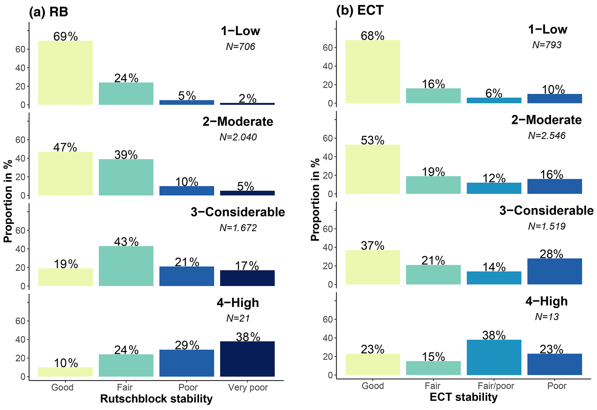
We analyzed the stability distributions obtained with the RB test at danger levels 1-Low to 4-High (Fig. 3a). At 4-High, very few RB tests were observed. The proportion of very-poor-rated RB tests increased monotonically with increasing danger level from 2 % at 1-Low to 38 % at 4-High (Fig. 3a). As a consequence, the combined proportion of very-poor-rated and poor-rated tests also increased strongly from 7 % to 67 %, while the proportion of tests rated as good decreased accordingly (69 % to 10 %; Fig. 3a). These patterns were also confirmed when exploring the correlation between the RB stability class and danger level (Spearman's rank-order correlation; ρ=0.4, p<0.001).

Figure 3 Distribution of stability ratings for the stability tests (a) rutschblock (RB) and (b) the ECT for danger levels 1-Low to 4-High. For the definition of the stability classes refer to Fig. 1 and Sect. 3.1. Note the small N for 4-High for both tests.

4.1.2 Frequency classes of very poor snowpack stability

Here, we describe the four frequency classes based on the frequency of very poor stability as sampled from the stability distributions shown in Fig. 3a (bootstrap sample size n=25). Regarding the sampling and the class definition procedure, refer to Sect. 3.2 and 3.3; regarding the sensitivity of these settings on the results, refer to Sect. 4.6.

Using four frequency classes, and labeling them none or nearly none, a few, several, and many, the thresholds in the proportion of very poor stability between frequency class labels were 0 %, 4 %, and 20 %, respectively (Table 2). This corresponded to a median proportion for very poor stability observed in each frequency class of 0 %, 4 %, 12 %, and 32 % or, if expressed in the number of very poor rutschblock test results, to 0, 1, 3, or 8 RB tests out of 25 drawn.

Large proportions of very poor stability (e.g., ≥50 %) occurred in less than 1 % of the sampled distributions, despite sampling a comparably large number of tests from 4-High, where very poor stability test results are more frequent (Fig. 3a), and using a low n in each of the bootstrap samples, which increases the variation in the sampled proportions.

The correlation between the frequency class describing the frequency of very poor stability and the danger level was strong (ρ=0.81, p<0.001; Fig. 4). For instance, the frequency class none or nearly none was most frequently sampled from stability tests observed at 1-Low (61 % of the cases). Similarly, the frequency class a few resulted most often when tests were sampled from 2-Moderate (47 %), the class several most often from 3-Considerable (56 %), and the class many most often from 4-High (86 %; Fig. 4). Hence, when the proportion of very poor stability was classified as many, this was, by itself, a strong indicator that the danger level was 4-High.

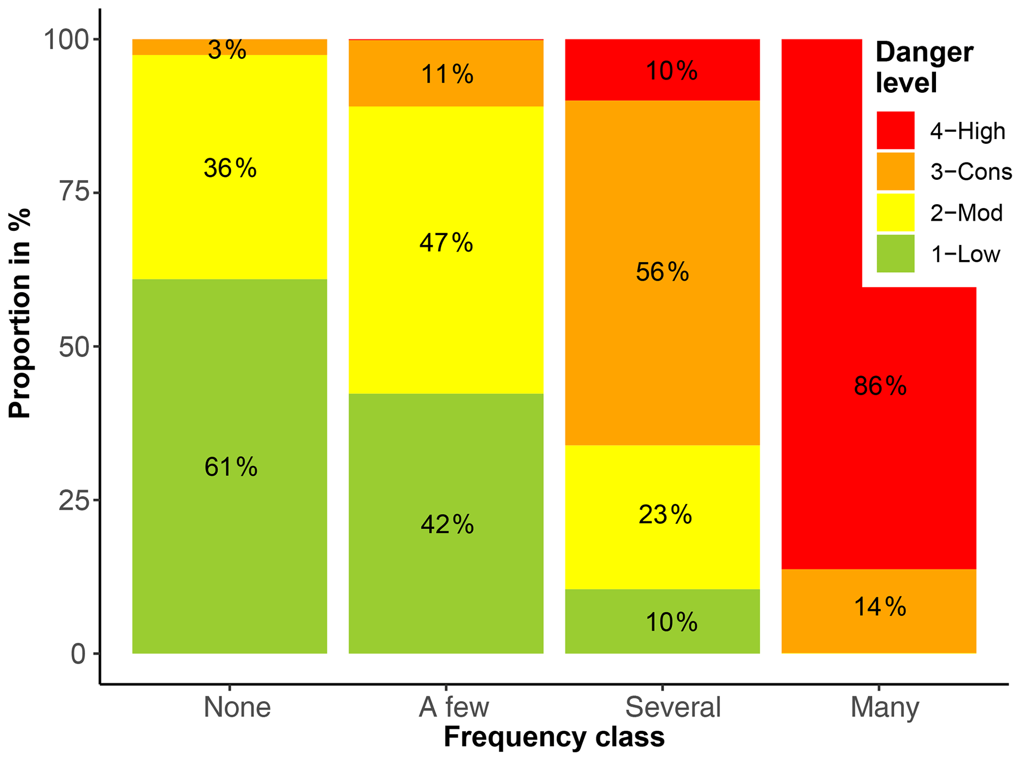
Figure 4 Distribution of the danger levels for the four frequency classes describing the proportion of very poor snowpack stability, derived from sampling 25 rutschblock tests (as described in Sect. 3.2). The respective proportions are indicated for each of the four danger levels.

Table 2 Frequency classification derived from the proportion of very poor stability ratings, using four frequency classes. The intervals for the frequency of very poor stability are shown. D(1st) and D(2nd) indicate the most frequent and second-most-frequent danger level the samples were drawn from, respectively. Also shown is the classification of the combination of stability class and frequency class based on the two most frequent danger levels, denoted as letters A to F, which will be used in Figs. 6 and 7. For class none or nearly none, no letter is assigned, as the next highest stability class should be considered.

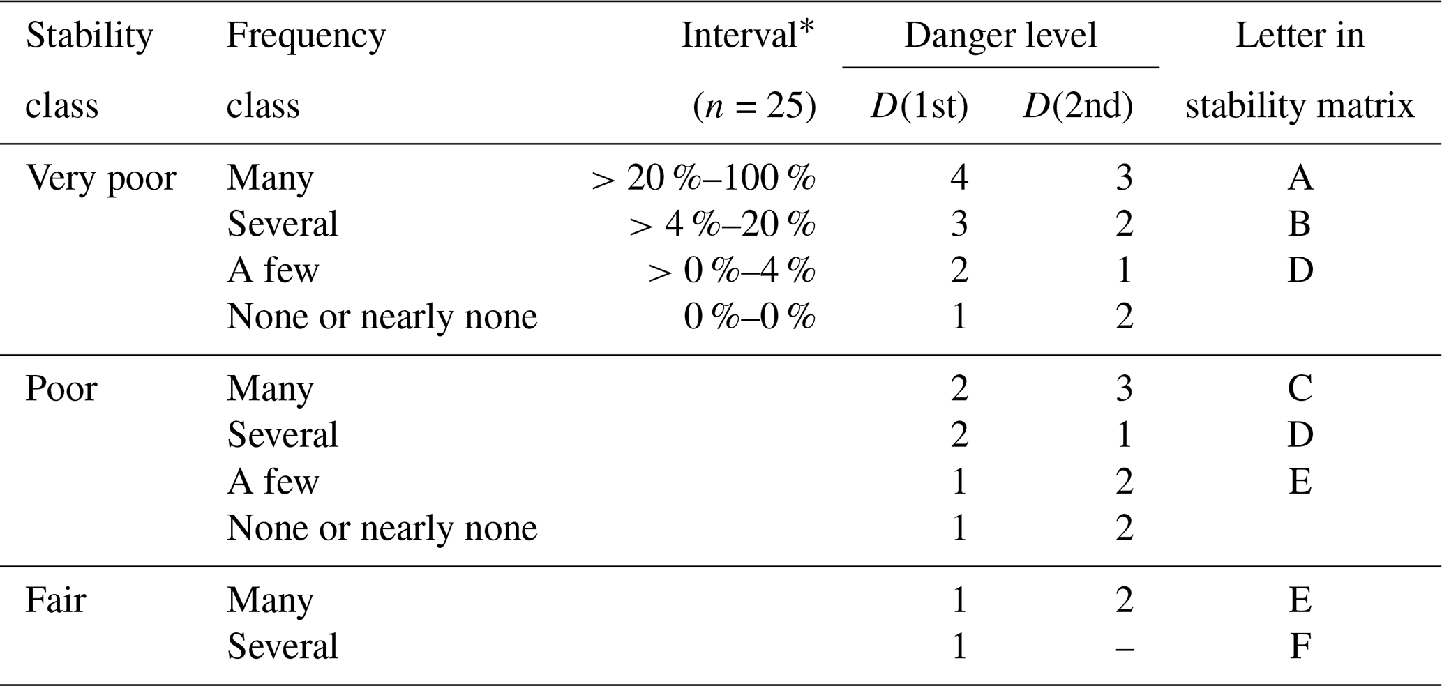
^* The thresholds indicated in the table are rounded according to the resolution of the test statistic, which depends on the number n of samples drawn in each bootstrap. Rounded to one decimal space, the interval thresholds for the frequency of very poor stability for sampling with n=25 were 0 %, 1.8 %, 6.2 %, 21 %, and 100 %.

4.2 Avalanche size

Most avalanches in the Swiss data set were size 1 (Fig. 5a), except at 4-High, where a similar proportion of size 1, 2, and 3 avalanches were reported. The proportion of size 1 avalanches decreased with danger level from 64 % to 32 %, while the combined proportion of size 3 and 4 avalanches was highest at 4-High with 39 %. Comparing the distributions at 1-Low to 3-Considerable shows that the most frequent avalanche size has little discriminating power to differentiate between danger levels. The median avalanche size was size 1 at 1-Low and 2-Moderate, size 1 to size 2 at 3-Considerable, and size 2 at 4-High (Fig. 5a).

Considering the size of the largest reported avalanche per day and warning region showed that the largest avalanche per day and region was most frequently size 2 for 1-Low and 2-Moderate, a mix of size 2 and size 3 at 3-Considerable, and size 3 at 4-High (Fig. 5b). The proportion of days when size 1 avalanches were the largest observed avalanche decreased significantly with increasing danger level (from 33 % to 1 %, p<0.001), while the proportion of days with at least one size 3 or size 4 avalanche increased significantly (from 20 % to 78 %, p<0.001). At 4-High, almost 80 % of the days had at least one avalanche of size 3 or 4 recorded.
The correlation between the size of the avalanche and the danger level was weak for the median size per day and warning region (ρ=0.15, p<0.001) but somewhat higher for the largest size (ρ=0.25, p<0.001).

Note that we did not explore days with no avalanches as we were interested in the size of avalanches and not their frequency. The frequency component is addressed using the frequency of locations with very poor stability as a proxy.

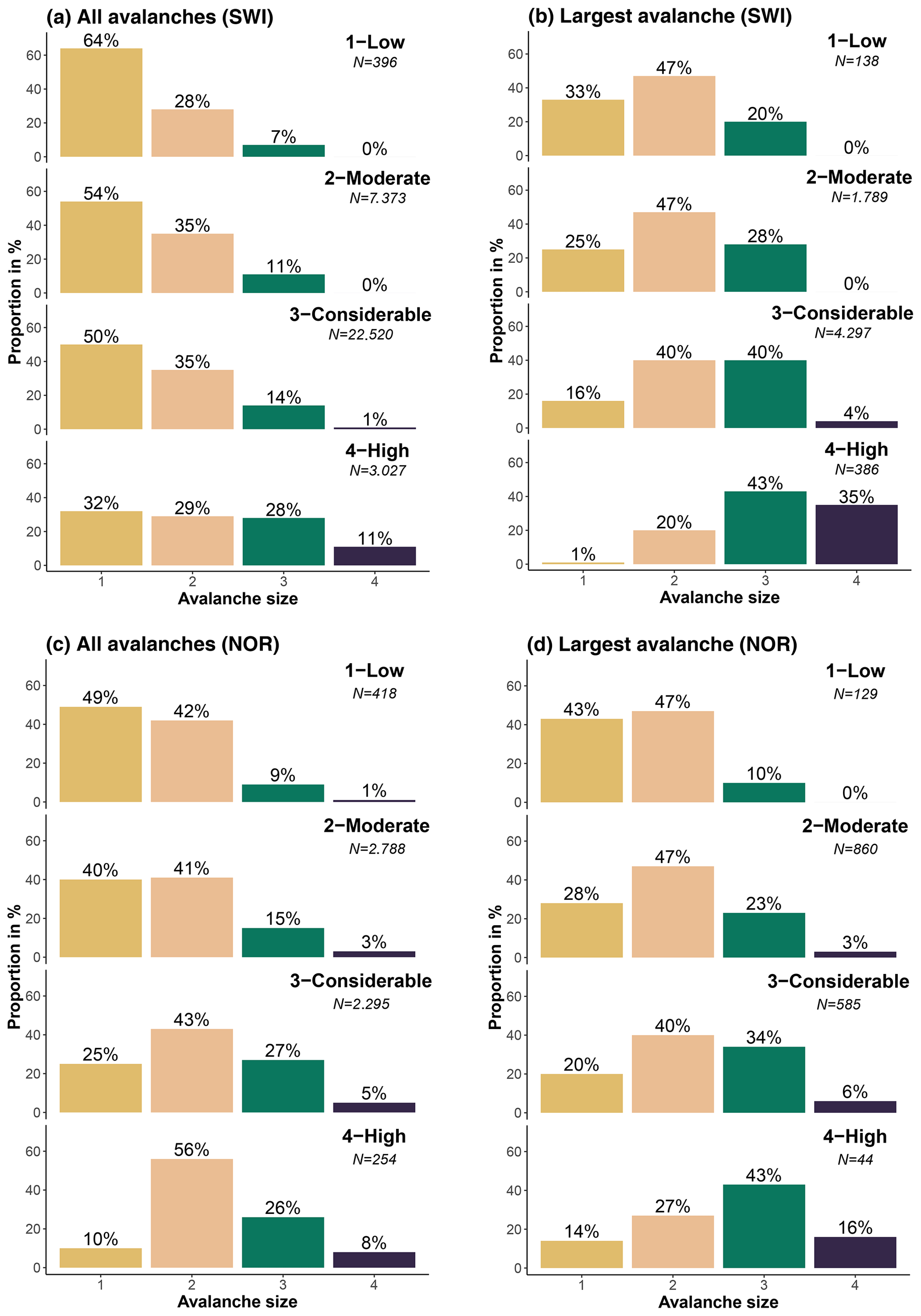
Figure 5 Size distribution of dry-snow avalanches, which released naturally or were human-triggered for danger levels 1-Low to 4-High, showing all avalanches (a, c) and the largest reported avalanche per day and warning region (b, d) in Switzerland (SWI; a, b) and Norway (NOR; c, d).

4.3 Combining the frequency of very poor stability and avalanche size

Assuming that the stability class very poor corresponds to the actual trigger locations, we combined the snowpack stability class, the frequency of this stability class, and avalanche size. Hence, this combination considers all three key factors characterizing the avalanche danger level. The resulting simulated data set contained the following information: danger level, frequency class describing occurrence of very poor stability, and largest avalanche size. These data looked like the following, here for 1-Low:
Sample 1 – 1-Low, a few, largest avalanche size 1
Sample 2 – 1-Low, none or nearly none, largest avalanche size 2
Sample 3 – 1-Low, a few, largest avalanche size 1
…
Sample B – 1-Low, none or nearly none, largest avalanche size 1.

Table 3 summarizes the simulated data set. The most frequent combinations of the frequency class and avalanche size for each danger level were as follows:

• 1-Low. None or nearly none locations with very poor stability (53 % of samples) existed. The largest avalanches were size 2 (48 %).

• 2-Moderate. A few locations with very poor stability (37 %) were present. The typical largest avalanche was of size 2 (50 %).

• 3-Considerable. Several locations with very poor stability (75 %) existed. The typical largest avalanches were sizes 2 or 3 (79 %).

• 4-High. Many locations with very poor stability (86 %) existed. The typical largest avalanche was of size 3 (43 %).

Table 3 Table showing the combination of the frequency class of very poor snowpack stability and the largest avalanche size for the four danger levels. Frequencies are rounded to the full percent value. Bold values highlight the most frequent combination; “–” indicates that these combinations did not exist.

^* None or nearly none. Simulation setting: rutschblock, avalanches (SWI), n=25, k=4, and B=2500 per danger level.

4.4 Data-driven look-up table for danger level assessment

Finally, we present a data-driven look-up table to assess avalanche danger (Fig. 6) using the simulations presented before. We used a stepwise approach and two matrices as proposed by Müller et al. (2016) in the so-called Avalanche Danger Assessment Matrix (ADAM).

The first matrix (Fig. 6a), which we refer to as the stability matrix, combines snowpack stability and the frequency class of the most unstable stability class observed. Cell labels (letters A to E) in this matrix were assigned based on similar danger level distributions behind the respective stability class–frequency class combination (Table 2). The letters reflect combinations with the most frequent and second-most-frequent danger levels in descending order with A being the highest and E the lowest danger level. Letter F in Table 2, a rare occurrence in our data, was combined with letter E. For class none or nearly none, no letter is assigned, as the next highest stability class should be considered. The mean simulated RB stability class distributions behind these cells are shown in Fig. 7a.

The second matrix (Fig. 6b), which we refer to as the danger matrix, combines snowpack stability and frequency with the largest avalanche size. The danger matrix displays the most frequent danger level (bold) and the second-most-frequent danger level characterizing this combination. If the second-most-frequent danger level was present in more than 30 % of the cases, the value is shown with no parentheses; if it was present in between 15 % and 30 %, it is placed in parentheses. To illustrate the actual danger level distributions behind this matrix, Fig. 7b summarizes the simulated data.

To derive the danger level, these two matrices can be used as follows:

1. In the stability matrix (Fig. 6a), the frequency class of very poor snowpack stability is assessed. If the frequency class was none or nearly none, the frequency class of poor snowpack stability is assessed. If the frequency class was again none or nearly none, the frequency class of fair snowpack stability is assessed.

2. The resulting letter is transferred to the danger matrix (Fig. 6b), where it is combined with the largest avalanche size (Fig. 6b).

3. The most frequent danger levels that were typical for this combination are shown.

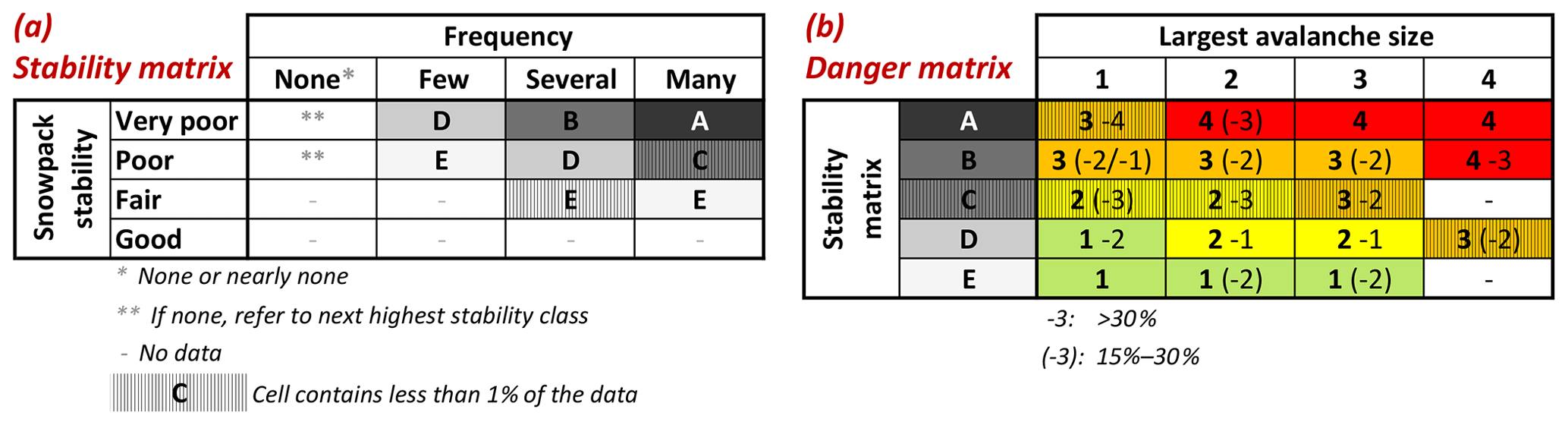
Figure 6 Data-driven look-up table for avalanche danger assessment (similar to the structure proposed by Müller et al., 2016). (a) The stability matrix combines the frequency class of the most unfavorable snowpack stability class (columns) and the snowpack stability class (rows) to obtain a letter describing specific stability situations. (b) The danger matrix combines the largest avalanche size (columns) and the specific stability situations (letter) obtained in the stability matrix (rows) to assess the danger level. In (b) the most frequent danger level is shown in bold. If the second-most-frequent danger level was present in more than 30 % of the cases, the value is shown with no parentheses; if it was present in between 15 % and 30 %, it is placed in parentheses. In (a) and (b) cells containing less than 1 % of the data are marked.

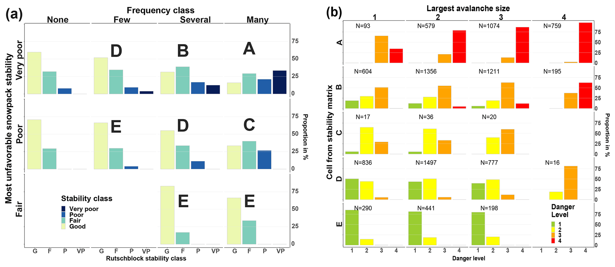
Figure 7 Data behind the matrices shown in Fig. 6. The layout of the columns and rows is identical to Fig. 6. The left panel (a) shows the mean simulated stability distributions behind the stability matrix (Fig. 6a). Letters describe cells with the corresponding most frequent and second-most-frequent danger level. In the right panel (b), the distribution of danger levels for combinations of the typical largest avalanche size and the letters obtained before in the stability matrix (A–E, Fig. 6a) are shown. The most frequent and second-most-frequent danger levels in each cell–avalanche size combination are shown in the danger matrix in the right part of Fig. 6b.

4.5 Comparison with other data sets

For the main results, presented in Sect. 4.1 to 4.4, we relied on stability test results and avalanche data from Switzerland. In the following, we compare these stability and avalanche size distributions to other data sets.

4.5.1 Snowpack stability distributions – comparing RB with ECT results

Additionally to the RB test, we explored stability distributions derived from ECT results and performed not only in Switzerland but also in Norway at 1-Low to 4-High (Fig. 3b).

The proportion of poor-rated ECTs increased from 10 % at 1-Low to 28 % at 3-Considerable, while the proportion of the two most unfavorable stability classes combined rose from 16 % to 42 %. At 4-High, where very few ECTs were observed, only the combined proportion of the two most unfavorable classes showed this increasing trend (61 %; Fig. 3b). Again, a positive though weak correlation between stability rating and danger level was noted (ρ=0.22, p<0.001).

In comparison to the RB test (Fig. 3a, Sect. 4.1.1), the ECT showed less distinct changes in the frequency of the most unstable and most stable classes between danger levels, and hence the correlation with the danger level was lower (ECT ρ=0.22 vs. RB ρ=0.4).

4.5.2 Avalanche size – comparing Swiss and Norwegian avalanche size distributions

The avalanche size distributions in Sect. 4.2, based on observations made in Switzerland (SWI; Fig. 5a, b), were compared to observations in Norway (NOR; Fig. 5c, d).

In Norway, size 1 was the most frequently reported size at 1-Low, while size 2 avalanches were the most frequent size at 3-Considerable and 4-High (Fig. 5c). The proportion of reported size 1 avalanches decreased with increasing danger level (from 49 % to 10 % from 1-Low to 4-High), while size 3 and 4 avalanches increased proportionally (from 10 % to 34 %). Similarities between Switzerland and Norway included a decreasing proportion of size 1 avalanches and increasing proportions of size 3 or 4 avalanches with danger level. Notable differences were primarily related to the proportion value: considering all reported avalanches, size 1 avalanches were proportionally less frequent in Norway than in Switzerland (NOR 17 %, SWI 30 %), while size 4 avalanches had larger proportions in Norway (NOR 2 %, SWI 1 %). This difference is likely linked to a lower reporting rate of smaller avalanches in Norway.

Considering the largest avalanche per day and warning region, Norway (Fig. 5d) showed similar trends in the size distributions to those in Switzerland (Fig. 5b). The proportion of size 1 avalanches decreased with increasing danger level, while size 3 and 4 avalanches increased. Size 2 avalanches were the most frequent at 1-Low to 3-Considerable. At 4-High, the largest reported avalanche was typically a size 3 avalanche. Differences between the Norwegian and the Swiss data were again primarily related to the proportion values. For instance, the proportion of size 1 avalanches as the largest reported avalanche decreased from 1-Low to 4-High from 43 % to 14 % in Norway, compared to 33 % to 1 % in Switzerland. Differences were also observed for the proportion of size 3 and 4 avalanches as the largest observed avalanche: their proportion increased from 1-Low to 4-High from 10 % to 59 % in Norway and from 20 % to 78 % in Switzerland.

4.6 Bootstrap sampling and frequency class definitions – sensitivity analysis

4.6.1 Bootstrap sampling

To obtain a variety of frequency distributions of point snow instability, we sampled stability ratings as described in Sect. 3.2. As outlined there, one important parameter affecting such a sampling approach is the number of stability ratings n drawn in each sample (sample size). In the following, we illustrate the effect of the bootstrap sample size n.

Influence of sample size

The results shown in Sect. 4.1, 4.3, and 4.4 were based on a sample size n = 25. To explore the effect of sample size, we in addition sampled using $n=\mathit{\{}\mathrm{10},\mathrm{25},\mathrm{50},\mathrm{100},\mathrm{200},\mathrm{1000}\mathit{\}}$. The histograms displaying the simulated proportion of very poor stability for various n irrespective of danger level showed that the distribution of the proportion of very poor stability was skewed towards lower proportions being more frequent than higher proportions, regardless of n (two examples for n=25 and n=200 are shown in Fig. 8a and c, respectively). Checking for multimodality in the histograms by visual inspection and by applying the modetest function (Ameijeiras-Alonso et al., 2018) showed that increasing the sample size n impacted the number of modes detected in the histograms, with two or more modes being present when n reached values of about 50. In the examples showing the proportions of very poor stability (Fig. 8), the number of modes increased from one for n=25 (Fig. 8a) to three for n=200 (Fig. 8c). Furthermore, the resulting simulations were visually checked for clusters in a two-dimensional context by considering the two extreme stability classes, the proportion of very poor and good stability ratings (Fig. 8b and d). Again, it can be noted that not only do the sampled distributions become visually more and more clustered with increasing n but the overlap between danger levels decreases. In the examples shown, no obvious clustering can be noted for n=25 while four distinct clusters exist when sampling n=200 tests in each bootstrap. This decrease in variance with increasing n, which leads to less overlap in samples drawn from different danger levels, is a characteristic of bootstrap sampling.

Figure 8 Simulated proportions of very poor and good snowpack stability derived from RB tests for different number of samples n drawn in each of the bootstraps (a and b: n=25, c and d: n=200). In the histograms (a, c) the proportion of very poor stability is shown; in the scatterplots (b, d) the most frequent danger level for a combination of very poor and good stability is shown. Note, the histogram in (a) is identical to Fig. 2c. The larger the sample size n, the more the data became multimodal and clustered around the means of each danger level. This is indicated by the p value (modetest, median p value of 10 repetitions, Ameijeiras-Alonso et al., 2018) in (a) and (c).

Plausibility of sampled distributions – comparison with observations

When introducing the bootstrap-sampling approach to create a range of plausible stability distributions (Sect. 3.2), we had to assume that a single stability rating is just one sample from the stability distribution on that day and that different days with the same danger level exhibit a range of similar stability distributions. Referring to Fig. 9, it can be noted that a range of typical distributions were indeed obtained for the four danger levels. For instance, for n=25 and 3-Considerable, the interquartile range of the simulated proportions of very poor stability was between about 10 % and 20 % (Fig. 9d) and for good stability between about 15 % and 30 % (Fig. 9f).

Comparing the bootstrap-sampled distributions with actually observed distributions of stability ratings on the same day and in the same region (N=41) showed that the distributions obtained using bootstrap sampling reflected the variation in the observed distributions reasonably well (Fig. 9). The exception was n=10 and good stability (Fig. 9c): in this case, the observed proportions of good stability were significantly different than the sampled distributions at 2-Moderate and 3-Considerable (p<0.05, Wilcoxon rank sum test).

In all examples shown in Fig. 9, the influence of a low number n of tests drawn in the bootstrap or from the distribution of stability ratings actually collected in the field is reflected in not only the large overlap in the proportions of a specific stability rating between danger levels but also the variation within danger levels.

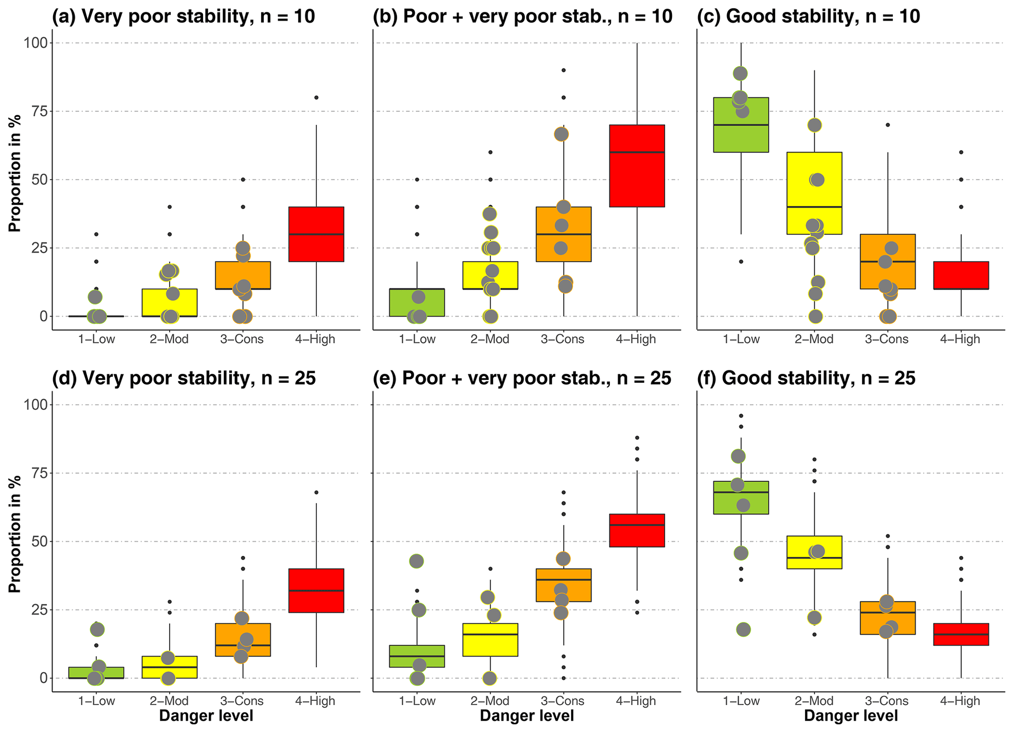
Figure 9 Comparison of observed (points, N=41) and bootstrap-sampled distributions (boxes) for the proportion of very poor (a, d), very poor and poor combined (b, e), and good (c, f) stability tests, for two settings of the number n of tests drawn. When 7 to 15 RB tests were observed on the same day and within the same region, these are shown together with sampled distributions using n=10 (a–c). When more than 16 tests were collected, these are shown together with sampled distributions using n=25 (d–f).

4.6.2 Frequency class definition

Relevant parameters for the definition of class intervals, as introduced in Sect. 3.3, are the respective median proportion of very poor stability VP_med and the number of classes k desired.

VP_med was affected by the resolution of the test statistic for very low values of n. For instance, for n=10, the resolution was 0.1 and VP_med was 0.1. For all other n values tested, VP_med was 0.08 or 0.085, despite large differences in the resolution of the test statistic (e.g., 0.04 for n=25 and 0.005 for n=200). The number of classes k desired, however, influenced the class interval definition as described in Sect. 3.3, as both the initial (lowest) class width a and the factor b, scaling the increase in interval width, decreased with k. However, for n≤50 and all k values tested, the initial (lowest) class contained only values for the proportion of very poor equaling 0. A value of k=4 seemed most suitable, as the resulting three lower class intervals would contain values for sampling with n>10. In all cases, an additional class would exist, generally at values between 0.5 and 0.9. As this class would remain empty most of the time, this class was merged with the respective lower one, thus expanding the upper interval limit of class many to 1.

The correlation between the frequency class and the danger level increased with increasing k and was strong even with n=10, with a large amount of overlap between classes (ρ>0.7, p<0.001).

5 Discussion

In the following, we discuss our findings in the light of potential uncertainties linked to the data (Sect. 5.1) and methods selected (Sect. 5.2). Furthermore, we compare the results to currently used definitions, guidelines, and decision aids used in regional avalanche forecasting (Sect. 5.3).

5.1 Data

5.1.1 Stability tests

Stability tests conducted by specifically trained observers are often performed at locations where the snowpack stability is expected to be low, though in an environment where spatial variability in the snowpack can be high (e.g., Schweizer et al., 2008a). Moreover, in most cases just one stability test was performed by an observer, not permitting us to judge whether this test was representative of the conditions of the day. However, the overall distributions of the stability ratings derived from RB or ECT results (Fig. 3) highlight the increase in locations with low snowpack stability with increasing danger levels.

At 4-High, stability test data were limited, as not only are these situations rare and temporally often short-lived but also backcountry travel in avalanche terrain is dangerous and therefore not recommended. As a consequence, not only were considerably fewer field observations made but also these were dug on less steep slopes at lower elevation, which may potentially underestimate snow instability.

5.1.2 Avalanche observations

We relied on observational data recorded in the context of operational avalanche forecasting. This means that differences in the quality of single observations are possible. For instance, variations in both the estimation of avalanche size (Moner et al., 2013) and locally assessing the avalanche danger level (Techel and Schweizer, 2017) have been noted. Furthermore, observations of avalanche activity often have a temporal uncertainty of a day or more, especially in situations with prolonged storms and poor visibility that often accompany a higher danger level. We addressed these issues by filtering the most extreme 2.5 % of the avalanche observations for each danger level.

Completeness of observations is another issue. Avalanche recordings are generally incomplete, in the sense that not all avalanches within an area are recorded as well as that single observations may lack information, e.g., on size. However, the size distributions (Fig. 5) reflect that smaller avalanches are more frequent, which was also observed in previous studies where other recording systems were applied such as recording of avalanches by snow safety staff and the public (Logan and Greene, 2018), manual mapping of avalanches (Hendrikx et al., 2005; Schweizer et al., 2020), or satellite-detection of avalanches (Eckerstorfer et al., 2017; Bühler et al., 2019). Still, smaller avalanches may be underrepresented compared to larger avalanches – as was the case for instance for size 1 avalanches in the Norwegian data set (Fig. 5c). This underreporting may depend not only on the relevance to an observer but also on the ease of recording or limitations set by the recording of numerous smaller avalanches. Since we did not primarily use the number of avalanches but instead focused on the largest avalanche per day and warning region, we expect this limitation to be less relevant.

To address potential bias in observations linked to Swiss observational standards (e.g., Techel et al., 2018), we compared findings with data from Norway. This brought additional challenges, like a different structure or different content of the observational data, which required us to make further assumptions (e.g., for counting the number of avalanches reported in forms when several avalanches were reported together in Norway). However, the largest avalanche size per day and warning region (Fig. 5b and d) showed similar overall patterns across countries, with increasing frequencies of very poor stability and increasing avalanche size with increasing danger level.

Finally, stability test results, avalanche observations, and local danger level estimates are generally not independent from each other, as often the same observer provided all this information. However, as shown by Bakermans et al. (2010), stability test results – compared to other observations – have relatively little influence on a local danger level estimate, while observations of natural or artificially triggered avalanches are unambiguous evidence of instability and may thus raise the quality of the local assessment.

5.2 Methods

5.2.1 Stability classification of the RB test and ECT

We relied on existing RB and ECT classifications (RB – Schweizer and Wiesinger, 2001; Schweizer, 2007a; ECT – Techel et al., 2020, Fig. 1). While the RB classification scheme is well-established in the operational assessment of snow profiles in the Swiss avalanche warning service, the classification of the ECT into four stability classes has only recently been proposed by Techel et al. (2020). They showed that for a large data set of pairs of ECTs and RB tests performed in the same snow pit, both classifications provided good correlations to slope stability. However, as shown by Techel et al. (2020), the most favorable and the most unfavorable RB stability classes captured slope stability better than the respective ECT classes, indicating a lower agreement between slope stability and ECT results compared to the RB results. This was our argument for not fully aligning the four RB and ECT stability classes and is supported by our findings: the RB stability class distributions changed more prominently from 1-Low (69 % good stability, 2 % very poor) to 4-High (10 % good, 38 % very poor) than the most favorable and unfavorable ECT stability classes (1-Low – 68 % good stability, 10 % poor; 4-High – 23 % good, 23 % poor).

5.2.2 Simulation of stability distributions

We could not rely on a large number of stability tests observed on the same day in the same region, which is a general problem in avalanche forecasting. We therefore generated stability distributions using resampling methods (Sect. 3.2) and by selecting sampling settings which lead to considerably overlapping distributions (Fig. 9). We argue that some overlap in stability distributions would characterize the large variability in avalanche conditions. However, we do not know which number n of stability tests drawn captures the variation best. We suppose that a combination of (labor-intensive) field measurements combined with spatial modeling in a large variety of avalanche conditions will be necessary to shed some light on this question (e.g., Reuter et al., 2016, for a small basin in Switzerland). Alternatively, spatial modeling of the snowpack, provided that a robust stability parameter can be simulated, would be required.

Repeated sampling from small data sets may underestimate the uncertainty associated with a metric, but more importantly, the question must be raised whether the sample reflects the population well. While at 1-Low to 3-Considerable, we sampled from between 700 and 2000 RB stability ratings per danger level, at 4-High the number of observations was very small (N=21). Hence, both the data shown in Fig. 3 and the sampled stability distributions for this danger level are more uncertain than for the other danger levels. While the combined number of locations with very poor and poor stability increased and those with good stability decreased at 4-High (Fig. 3), judging whether the observed tests reflect the population well is difficult. Unfortunately, we are not aware of other studies that have explored the snowpack stability distribution in a region at 4-High based on many tests, and therefore we have no comparison. Even on 7 February 2003, one of the days of the verification campaign in the region of Davos, Switzerland (Schweizer et al., 2003), the forecast danger level 4-High was verified to be between 3-Considerable and 4-High (Schweizer, 2007b). On this day, 14 rutschblock tests were observed. Of these, 36 % were either very poor or poor, thus being close to the average values noted for 3-Considerable (Fig. 3a). We did not consider these data, as we did not analyze data when they were for intermediate danger levels.

Comparing the distributions of our snowpack stability classes with the characteristic stability distributions obtained during the verification campaign in Switzerland in 2002 and 2003, some differences can be noted (Swiss RB data). For instance, the proportion of very poor and poor combined was at 2-Moderate about 15 % and at 3-Considerable about 40 %, which is lower than findings (20 %–25 % and about 50 %, respectively) by Schweizer et al. (2003). At 1-Low, about 70 % of the RB tests were classified as good, while Schweizer et al. (2003) noted about 90 % of the profiles to have good or very good stability. This suggests a smaller spread in the distribution of our automatically assigned stability classes, compared to the manual classification approach according to Schweizer and Wiesinger (2001).

5.2.3 Classification of snowpack stability frequency distributions

In addition to simulating snowpack stability distributions using a resampling approach, we developed a data-driven classification of the proportion of very poor stability tests. Our approach shows that the number n drawn for each bootstrap has little influence on class interval definitions, as long as the resolution of the test statistic is sufficiently high. Class thresholds are primarily defined by the central tendency of the distribution, in our case the median proportion of very poor stability tests VP_med, and by the number of classes preferred k.

Assigning a class to the proportion of very poor stability, however, was affected by n due to the fact that n influences both the resolution of the statistic and the variance. This means that conceptually we can think in frequency classes, as long as class interval boundaries are scaled according to the data used. This need to scale class intervals according to the data source, however, also implies that there is no unique set of values which could be used. Furthermore, the simulated stability distributions indicate that the focus is on optimizing class definitions to values between 0 % and 40 % when relying on stability tests, rather than the entire potential parameter space (0 %–100 %).

The preferred number of classes k may depend on a number of factors. We suggest that defining k should be guided by keeping classes as distinguishable as possible – for instance by addressing the frequently occurring low proportions of very poor stability on the one hand, the rarely observed large proportions of very poor stability on the other hand, and potentially a class covering the proportions in between. Furthermore, these terms must be unambiguously understandable to the user, regardless of language.

5.3 Data interpretation

5.3.1 Snowpack stability and frequency distribution of snowpack stability

We showed an increasing frequency (or number of locations) of very poor snowpack stability with increasing danger level, in line with previous studies exploring point snowpack stability within a region or small basin (Schweizer et al., 2003; Reuter et al., 2016) or the number of natural and human-triggered avalanches within a region (e.g., Schweizer et al., 2020). Furthermore, we showed that high frequencies of very poor stability (≥30 %) were comparably rare (15 % of the simulated distributions). Even at 4-High, less than 4 % of the distributions had frequencies of very poor stability ≥50 %.
We explored snowpack stability using RB tests and ECTs, which describe the stability at a specific point. However, within a slope or a region, point snowpack stability is variable (e.g., Birkeland, 2001; Schweizer et al., 2008a). In avalanche forecasts this can be expressed by the frequency a certain stability class existing and by additionally describing the locations more specifically. When describing the avalanche danger level in a region, snowpack stability and the frequency distribution of snowpack stability must therefore be considered. We suggest that primarily the frequency of the lowest stability class is relevant for assigning a danger level, as this stability class combined with the frequency of this stability class describes the minimal trigger needed to release an avalanche and how frequently these most unstable locations exist within a region. These two factors must therefore be assessed in combination for all aspects and elevations. Furthermore, the specific description of triggering locations, for instance at the treeline or in extremely steep terrain, may provide an indication of where in the terrain these locations may exist more frequently within their frequency classes. Even though different terms are used, both the EAWS Matrix (EAWS, 2017) and the CMAH (Statham et al., 2018a) first combine snowpack stability and the frequency distribution of snowpack stability before avalanche size is considered. The respective terms which were used are the “load” (trigger) and the “distribution of hazardous sites” in the EAWS Matrix and the “sensitivity to triggers” and “spatial distribution” leading to the “likelihood of avalanches” in the CMAH.

We explored primarily the frequency of the stability class very poor, which is most closely related to actual triggering points. However, as several studies have shown, even when stability tests suggested instability, often only some of the slopes were in fact unstable and released as an avalanche (e.g., Moner et al., 2008; Techel et al., 2020). Thus, depending on the data used to define very poor stability, for instance whether stability tests or natural avalanches are used and whether avalanches are observed from one location or using spatially continuous methods like satellite images, an adjustment of class intervals may be necessary to capture the frequency of locations where natural avalanches may initiate or where human-triggered avalanches are possible.

5.3.2 Avalanche size

The most frequent avalanche size had little discriminating power, with the typical size being size 1 or size 2, regardless of danger level. This can be explained by the fact that larger events normally occur less frequent than smaller events. This frequency–magnitude relation has also been observed for other natural hazards (e.g., Malamud and Turcotte, 1999) and has been described by power laws for avalanche size distributions (Birkeland and Landry, 2002; Faillettaz et al., 2004).

We showed that considering the largest avalanche per day resulted in a slightly better discrimination between danger levels. This finding is also supported by Schweizer et al. (2020), with the size of the largest avalanche being mostly of size 4 at 4-High. Furthermore, the typical largest expected avalanche is highly relevant for risk assessment and mitigation.

For danger level 5-Very High, for which we had no data, other studies have shown a further shift towards size  4 avalanches. Schweizer et al. (2020) showed that at 5-Very High, size 4 avalanches were 15 times more frequent than at 3-Considerable and 5 times more frequent compared to 4-High. In two extraordinary avalanche situations in January 2018 and January 2019, when danger level 5-Very High was verified for parts of the Swiss Alps, avalanches recorded using satellite data showed that often 10 or more size 4 avalanches and/or 1 size 5 avalanche were observed per 100 km² (Bühler et al., 2019; Zweifel et al., 2019).

5.3.3 Combining snowpack stability, the frequency distribution of snowpack stability, and avalanche size

In Sect. 4.3 we presented a data-driven look-up table to assess avalanche danger (Fig. 6). As can be seen in this table, the combination of snowpack stability and the frequency that best matches an avalanche situation (A to E) is highly relevant for danger level assessment. In general, avalanche size had a lesser influence on the danger level, once the cell describing stability was fixed, as might be anticipated. This is in contrast to the original avalanche danger level assessment matrix (ADAM; Müller et al., 2016) that proposed that an increase in either the frequency class or the avalanche size or a decrease in snowpack stability should lead to an increase in danger level by one level. Clearly, the presented data-driven look-up table (Fig. 6) highlights that a greater focus must be placed on snowpack stability and the frequency distribution of snowpack stability, compared to avalanche size, when assessing avalanche hazard. This was also shown by Clark (2019), who explored the combination of descriptive terms describing the three factors in the data behind the avalanche forecasts in Canada and their relation to the published danger level and avalanche problem. They showed that the “likelihood of avalanches”, which compares to our stability matrix (Fig. 6), also had a greater impact on the resulting danger level than avalanche size, even though avalanche size ≤1.5 (considered harmless to people) was often a first split in a decision tree model. Hence, despite using different approaches, partially different terminology, and slightly different avalanche danger scales in Europe and North America, the relative importance of the three key contributing factors and the distributions of the danger levels is similar.

Our approach can only provide general distributions observed under dry-snow conditions. The look-up table presented in Fig. 6 should therefore be seen as a tool (a) to aid in the discussion of specific situations and (b) to improve the definitions underlying the categorical descriptions of the danger levels.

6 Conclusions

We explored observational data from two different countries relating to the three key factors describing avalanche hazard: snowpack stability, the frequency distribution of snowpack stability, and avalanche size. We simulated stability distributions and defined four classes describing the frequency of potential avalanche-triggering locations, which we termed none or nearly none, a few, several, and many. The observed and simulated distributions of stability ratings derived from RB tests showed that locations with very poor stability are generally rare (Figs. 3a, 8a–d).

Our findings suggest that the three key factors did not distinguish equally prominently between the danger levels:

• The proportion of very poor or poor stability test results increased from one danger level to the next highest one (Figs. 3 and 9). Considering very poor snowpack stability and the frequency of this stability class alone, it already distinguished well between danger levels (Table 2, Fig. 4).

• Considering the largest observed avalanche size per day and warning region was most relevant to distinguishing between 3-Considerable and 4-High (Fig. 5 and Table 3). For other situations, the largest avalanche size – when used on its own – had less discriminating power to distinguish between danger levels 1-Low to 3-Considerable compared to the other two factors (the lowest stability class present and the frequency of this class; Fig. 5).

In summary, the frequency of the most unfavorable snowpack stability class is the dominating discriminator. At higher danger levels the occurrence of size 4 avalanches discriminates danger level 3-Considerable from 4-High. We further suppose that the occurrence of size 5 avalanches discriminates between 4-High and 5-Very High without a significant additional increase in the frequency of very poor stability. This shift in importance between factors is currently poorly represented in existing decision aids like the EAWS Matrix or ADAM (Müller et al., 2016) and also in the European Avalanche Danger Scale.

To combine the three factors and to derive avalanche danger, we introduced two data-driven look-up tables (Fig. 6), which can be used to assess avalanche danger levels in a two-step approach. In these tables, only the frequency of locations with the lowest snowpack stability is assessed, with no spatial component and combined with the largest avalanche size. Spatial information in avalanche forecasts includes the aspects and elevations where the frequency of locations with the lowest stability class exists and possibly terrain features within the frequency class where triggering is particularly likely.

We hope that our data-driven perspective on avalanche hazard will allow a review of key definitions in avalanche forecasting such as the avalanche danger scale.